AGENCY:
Office of Energy Efficiency and Renewable Energy, Department of Energy.
ACTION:
Final rule.
SUMMARY:
The Energy Policy and Conservation Act of 1975 (EPCA or the Act), as amended, prescribes energy conservation standards for various consumer products and certain commercial and industrial equipment. In addition to specifying a list of covered consumer products and commercial equipment, EPCA contains provisions that enable the Secretary of Energy to classify additional types of consumer products as covered products. On April 18, 2016, the U.S. Department of Energy (DOE or the Department) published a final coverage determination to classify portable air conditioners (ACs) as covered consumer products under the applicable provisions in EPCA. In this final rule, DOE establishes new energy conservation standards for portable ACs. DOE has determined that the energy conservation standards for these products would result in significant conservation of energy, and are technologically feasible and economically justified.
DATES:
The effective date of this rule is March 10, 2020. Compliance with the standards established for portable ACs in this final rule is required on and after January 10, 2025.
ADDRESSES:
The docket for this rulemaking, which includes Federal Register notices, public meeting attendee lists and transcripts, comments, and other supporting documents/materials, is available for review at www.regulations.gov. All documents in the docket are listed in the www.regulations.gov index. However, not all documents listed in the index may be publicly available, such as information that is exempt from public disclosure.
The docket web page can be found at https://www.regulations.gov/docket?D=EERE-2013-BT-STD-0033. The docket web page contains simple instructions on how to access all documents, including public comments, in the docket.
For further information on how to review the docket, contact the Appliance and Equipment Standards Program staff at (202) 586-6636 or by email: ApplianceStandardsQuestions@ee.doe.gov.
FOR FURTHER INFORMATION CONTACT:
Mr. Bryan Berringer, U.S. Department of Energy, Office of Energy Efficiency and Renewable Energy, Building Technologies Office, EE-5B, 1000 Independence Avenue SW, Washington, DC 20585-0121. Telephone: (202) 586-0371. Email: Bryan.Berringer@ee.doe.gov.
Ms. Sarah Butler, U.S. Department of Energy, Office of the General Counsel, GC-33, 1000 Independence Avenue SW, Washington, DC 20585-0121. Telephone: (202) 586-1777. Email: Sarah.Butler@hq.doe.gov.
SUPPLEMENTARY INFORMATION:
Table of Contents
I. Synopsis of the Final Rule
A. Benefits and Costs to Consumers
B. Impact on Manufacturers
C. National Benefits and Costs
D. Conclusion
II. Introduction
A. Authority
B. Background
III. General Discussion
A. Product Classes and Scope of Coverage
B. Test Procedure
C. Technological Feasibility
1. General
2. Maximum Technologically Feasible Levels
D. Energy Savings
1. Determination of Savings
2. Significance of Savings
E. Economic Justification
1. Specific Criteria
a. Economic Impact on Manufacturers and Consumers
b. Savings in Operating Costs Compared to Increase in Price
c. Energy Savings
d. Lessening of Utility or Performance of Products
e. Impact of Any Lessening of Competition
f. Need for National Energy Conservation
g. Other Factors
2. Rebuttable Presumption
F. Other Issues
IV. Methodology and Discussion of Related Comments
A. Market and Technology Assessment
1. Definition and Scope of Coverage
2. Product Classes
a. Preliminary Analysis and Notice of Proposed Rulemaking (NOPR) Proposals
b. Comments and Responses
3. Technology Options
B. Screening Analysis
1. Screened-Out Technologies
2. Additional Comments
3. Remaining Technologies
C. Engineering Analysis
1. Efficiency Levels
a. Baseline Efficiency Levels
b. Higher Energy Efficiency Levels
2. Manufacturer Production Cost Estimates
D. Markups Analysis
E. Energy Use Analysis
1. Consumer Samples
2. Cooling Mode Hours and Sensitivity Analyses
3. Fan-only Mode and Standby Mode Hours
F. Life-Cycle Cost and Payback Period Analysis
1. Product Cost
2. Installation Cost
3. Annual Energy Consumption
4. Energy Prices
5. Maintenance and Repair Costs
6. Product Lifetime
7. Discount Rates
8. Energy Efficiency Distribution in the No-New-Standards Case
9. Payback Period Analysis
G. Shipments Analysis
H. National Impact Analysis
1. Product Efficiency Trends
2. National Energy Savings
3. Net Present Value Analysis
I. Consumer Subgroup Analysis
J. Manufacturer Impact Analysis
1. Overview
2. Government Regulatory Impact Model (GRIM) and Key Inputs
a. Manufacturer Production Costs
b. Shipment Projections
c. Product and Capital Conversion Costs
d. Markup Scenarios
3. Discussion of Comments
K. Emissions Analysis
L. Monetizing Carbon Dioxide and Other Emissions Impacts
1. Social Cost of Carbon
a. Monetizing Carbon Dioxide Emissions
b. Development of Social Cost of Carbon Values
c. Current Approach and Key Assumptions
2. Social Cost of Methane and Nitrous Oxide
3. Social Cost of Other Air Pollutants
M. Utility Impact Analysis
N. Employment Impact Analysis
V. Analytical Results and Conclusions
A. Trial Standard Levels (TSLs)
B. Economic Justification and Energy Savings
1. Economic Impacts on Individual Consumers
a. Life-Cycle Cost and Payback Period
b. Consumer Subgroup Analysis
c. Rebuttable Presumption Payback
2. Economic Impacts on Manufacturers
a. Industry Cash Flow Analysis Results
b. Impacts on Employment
c. Impacts on Manufacturing Capacity
d. Impacts on Subgroups of Manufacturers
e. Cumulative Regulatory Burden
3. National Impact Analysis
a. Significance of Energy Savings
b. Net Present Value of Consumer Costs and Benefits
c. Indirect Impacts on Employment
4. Impact on Utility or Performance of Products
5. Impact of Any Lessening of Competition
6. Need of the Nation to Conserve Energy
7. Other Factors
8. Summary of National Economic Impacts
C. Conclusion
1. Benefits and Burdens of TSLs Considered for Portable AC Standards
2. Annualized Benefits and Costs of the Adopted Standards
VI. Procedural Issues and Regulatory Review
A. Review Under Executive Orders 12866 and 13563
B. Review Under the Regulatory Flexibility Act
C. Review Under the Paperwork Reduction Act
D. Review Under the National Environmental Policy Act of 1969
E. Review Under Executive Order 13132
F. Review Under Executive Order 12988
G. Review Under the Unfunded Mandates Reform Act of 1995
H. Review Under the Treasury and General Government Appropriations Act, 1999
I. Review Under Executive Order 12630
J. Review Under the Treasury and General Government Appropriations Act, 2001
K. Review Under Executive Order 13211
L. Review Under the Information Quality Bulletin for Peer Review
M. Congressional Notification
VII. Approval of the Office of the Secretary
I. Synopsis of the Final Rule
Title III, Part B [1] of the Energy Policy and Conservation Act of 1975 (EPCA or the Act), Public Law 94-163 (42 U.S.C. 6291-6309, as codified), established the Energy Conservation Program for Consumer Products Other Than Automobiles.[2] In addition to specifying a list of covered residential products and commercial equipment, EPCA contains provisions that enable the Secretary of Energy to classify additional types of consumer products as covered products. (42 U.S.C. 6292(a)(20)) In a final determination of coverage published in the Federal Register on April 18, 2016 (the “April 2016 Final Coverage Determination”), DOE classified portable ACs as covered consumer products under EPCA. 81 FR 22514.
Pursuant to EPCA, any new or amended energy conservation standard must be designed to achieve the maximum improvement in energy efficiency that DOE determines is technologically feasible and economically justified. (42 U.S.C. 6295(o)(2)(A)) Furthermore, the new or amended standard must result in significant conservation of energy. (42 U.S.C. 6295(o)(3)(B))
In accordance with these and other statutory provisions discussed in this document, DOE is adopting energy conservation standards for portable ACs. The standards, which correspond to trial standard level (TSL) 2 (described in section V.A of this document), are minimum allowable combined energy efficiency ratio (CEER) standards, which are expressed in British thermal units (Btu) per watt-hour (Wh), and are shown in Table I.1. These standards apply to all single-duct portable ACs and dual-duct portable ACs that are manufactured in, or imported into, the United States starting on January 10, 2025.

A. Benefits and Costs to Consumers
Table I.2 summarizes DOE's evaluation of the economic impacts of the adopted standards on consumers of portable ACs, as measured by the average life-cycle cost (LCC) savings and the simple payback period (PBP).[3] The average LCC savings are positive and the PBP is less than the average lifetime of portable ACs, which is estimated to be approximately 10 years (see section IV.F.6 of this document).
| Product class | Average LCC savings (2015$) | Simple payback period (years) |
|---|---|---|
| Single-duct and dual-duct portable air conditioners | 125 | 2.6 |
DOE's analysis of the impacts of the adopted standards on consumers is described in section IV.F of this document. DOE also performed three sensitivity analyses on its primary assertion that portable air conditioners are used and operated in a similar manner to room air conditioners to further analyze the effects of the benefits and cost to consumers from these products. In one sensitivity analysis, DOE found that reducing operating hours by 50 percent, resulted in an estimate of one-third of the energy cost savings relative to the primary estimate. In this low-usage case, the average LCC savings for all consumers under the adopted standards would be $35 (compared with $125 in the primary estimate), and 42 percent of consumers would be impacted negatively (compared with 27 percent in the primary estimate). The simple payback period would be 5.1 years (compared with 2.6 years in the primary estimate). Further details are presented in section IV.E, V.B.1, and appendix 8F and appendix 10E of the final rule TSD.
B. Impact on Manufacturers
The industry net present value (INPV) is the sum of the discounted cash flows to the industry from the base year through the end of the analysis period (2017-2051). Using a real discount rate of 6.6 percent, DOE estimates that the INPV for manufacturers of portable ACs in the case without new standards is $738.5 million in 2015$. Under the adopted standards, DOE expects the change in INPV to range from −34.3 percent to −28.8 percent, which is approximately −$253.4 million to −$212.4 million. In order to bring products into compliance with new standards, DOE expects the industry to incur total conversion costs of $320.9 million.
DOE's analysis of the impacts of the adopted standards on manufacturers is described in section IV.J and section V.B.2 of this document.
C. National Benefits and Costs 4
DOE's analyses indicate that the adopted energy conservation standards for portable ACs would save a significant amount of energy. Relative to the case without new standards the lifetime energy savings for portable ACs purchased in the 30-year period that begins in the anticipated year of compliance with the new standards (2022-2051), amount to 0.49 quadrillion Btu, or quads.[5] This represents a savings of 6.4 percent relative to the energy use of these products in the case without new standards (referred to as the “no-new-standards case”).
The cumulative net present value (NPV) of total consumer benefits of the standards for portable ACs ranges from $1.25 billion (at a 7-percent discount rate) to $3.06 billion (at a 3-percent discount rate). This NPV expresses the estimated total value of future operating-cost savings minus the estimated increased product costs for portable ACs purchased in 2022-2051.
In addition, the new standards for portable ACs are projected to yield significant environmental benefits. DOE estimates that the standards will result in cumulative emission reductions (over the same period as for energy savings) of 25.6 million metric tons (Mt) [6] of carbon dioxide (CO2), 16.4 thousand tons of sulfur dioxide (SO2), 32.2 tons of nitrogen oxides (NOX), 124.8 thousand tons of methane (CH4), 0.4 thousand tons of nitrous oxide (N2 O), and 0.06 tons of mercury (Hg).[7] The estimated reduction in CO2 emissions through 2030 amounts to 4.0 Mt, which is equivalent to the emissions resulting from the annual electricity use of more than 0.42 million homes.
The value of the CO2 reductions is calculated using a range of values per metric ton (t) of CO2 (otherwise known as the “social cost of carbon”, or SC-CO2) developed by a Federal interagency working group.[8] The derivation of the SC-CO2 values is discussed in section IV.L.1 of this document. Using discount rates appropriate for each set of SC-CO2 values, DOE estimates the present value of the CO2 emissions reduction is between $0.2 billion and $2.5 billion, with a value of 0.8 billion using the central SC-CO2 case represented by $40.6/metric ton (t) in 2015.
DOE also calculated the value of the reduction in emissions of the non-CO2 greenhouse gases (GHGs), CH4 and N2 O, using values for the social cost of methane (SC-CH4) and the social cost of nitrous oxide (SC-N2 O) recently developed by the interagency working group.[9] See section IV.L.2 for description of the methodology and the values used for DOE's analysis. The estimated present value of the CH4 emissions reduction is between $0.04 billion and $0.3 billion, with a value of $0.1 billion using the central SC-CH4 case, and the estimated present value of the N2 O emissions reduction is between $0.001 billion and $0.011 billion, with a value of $0.004 billion using the central SC-N2 O case.
DOE also estimates that the present value of the NOX emissions reduction to be $0.02 billion using a 7-percent discount rate, and $0.06 billion using a 3-percent discount rate.[10] DOE is still investigating appropriate valuation of the reduction in other emissions, and therefore did not include any such values in the analysis for this final rule.
Table I.3 summarizes the economic benefits and costs expected to result from the adopted standards for portable ACs.
| Category | Present value (billion 2015$) | Discount rate percent |
|---|---|---|
| Benefits | ||
| Consumer Operating Cost Savings | 1.8 | 7 |
| 4.1 | 3 | |
| GHG Reduction (using avg. social costs at 5% discount rate) **. | 0.2 | 5 |
| GHG Reduction (using avg. social costs at 3% discount rate) **. | 1.0 | 3 |
| GHG Reduction (using avg. social costs at 2.5% discount rate) **. | 1.5 | 2.5 |
| GHG Reduction (using 95th percentile social costs at 3% discount rate) **. | 2.9 | 3 |
| NOX Reduction † | 0.02 | 7 |
| 0.06 | 3 | |
| Total Benefits ‡ | 2.8 | 7 |
| 5.1 | 3 | |
| Costs | ||
| Consumer Incremental Installed Costs | 0.5 | 7 |
| 1.0 | 3 | |
| Total Net Benefits | ||
| Including GHG and NOX Reduction Monetized Value ‡ | 7 | |
| 4.1 | 3 | |
| * This table presents the costs and benefits associated with portable ACs shipped in 2022-2051. These results include benefits to consumers which accrue after 2051 from the products shipped in 2022-2051. The incremental installed costs include incremental equipment cost as well as installation costs. The costs account for the incremental variable and fixed costs incurred by manufacturers due to the proposed standards, some of which may be incurred in preparation for the rule. The GHG reduction benefits are global benefits due to actions that occur domestically. | ||
| ** The interagency group selected four sets of SC-CO2, SC-CH4, and SC-N2 O values for use in regulatory analyses. Three sets of values are based on the average social costs from the integrated assessment models, at discount rates of 5 percent, 3 percent, and 2.5 percent. The fourth set, which represents the 95th percentile of the SC-CO2 distribution calculated using a 3-percent discount rate, is included to represent higher-than-expected impacts from climate change further out in the tails of the social cost distributions. The social cost values are emission year specific. See section IV.L.1 of this document for more details. | ||
| † DOE estimated the monetized value of NOX emissions reductions associated with electricity savings using benefit per ton estimates from the Regulatory Impact Analysis for the Clean Power Plan Final Rule, published in August 2015 by EPA's Office of Air Quality Planning and Standards. (Available at www.epa.gov/cleanpowerplan/clean-power-plan-final-rule-regulatory-impact-analysis.) See section IV.L of this document for further discussion. DOE is primarily using a national benefit-per-ton estimate for NOX emitted from the electricity generating sector based on an estimate of premature mortality derived from the ACS study (Krewski et al. 2009). If the benefit-per-ton estimates were based on the Six Cities study (Lepuele et al. 2011), the values would be nearly two-and-a-half times larger. | ||
| ‡ Total Benefits for both the 3-percent and 7-percent cases are presented using the average social costs with 3-percent discount rate. | ||
The benefits and costs of the adopted standards, for portable ACs sold in 2022-2051, can also be expressed in terms of annualized values. The monetary values for the total annualized net benefits are (1) the reduced consumer operating costs, minus (2) the increases in product purchase prices and installation costs, plus (3) the value of the benefits of CO2 and NOX emission reductions, all annualized.[11]
The national operating cost savings are domestic private U.S. consumer monetary savings that occur as a result of purchasing the covered products and are measured for the lifetime of portable ACs shipped in 2022-2051. The benefits associated with reduced CO2 emissions achieved as a result of the adopted standards are also calculated based on the lifetime of portable ACs shipped in 2022-2051. Because CO2 emissions have a very long residence time in the atmosphere, the SC-CO2 values for CO2 emissions in future years reflect impacts that continue through 2300. The CO2 reduction is a benefit that accrues globally.
Estimates of annualized benefits and costs of the adopted standards are shown in Table I.4. The results under the primary estimate are as follows. Using a 7-percent discount rate for benefits and costs other than GHG reduction (for which DOE used average social costs with a 3-percent discount rate,[12] the estimated cost of the standards in this rule is $61 million per year in increased equipment costs, while the estimated annual benefits are $202.7 million in reduced equipment operating costs, $56.7 million in GHG reductions, and $2.6 million in reduced NOX emissions. In this case, the net benefit amounts to $201 million per year. Using a 3-percent discount rate for all benefits and costs, the estimated cost of the standards is $59 million per year in increased equipment costs, while the estimated annual benefits are $240.0 million in reduced operating costs, $56.7 million in GHG reductions, and $3.3 million in reduced NOX emissions. In this case, the net benefit amounts to $241 million per year.
| Discount rate (percent) | Primary estimate | Low-net- benefits estimate | High-net- benefits estimate | |
|---|---|---|---|---|
| (million 2015$/year) | ||||
| Benefits | ||||
| Consumer Operating Cost Savings | 7 | 202.7 | 99.1 | 214.4. |
| 3 | 240.0 | 116.3 | 256.1. | |
| CO2 Reduction (using avg. social costs at 5% discount rate) ** | 5 | 18.4 | 8.8 | 19.9. |
| CO2 Reduction (using avg. social costs at 3% discount rate) ** | 3 | 56.7 | 27.0 | 61.4. |
| CO2 Reduction (using avg. social costs at 2.5% discount rate) ** | 2.5 | 81.1 | 38.6 | 87.9. |
| CO2 Reduction (using 95th percentile SC-CO2 at 3% discount rate) ** | 3 | 169.9 | 80.9 | 184.1. |
| NOX Reduction † | 7 | 2.6 | 1.2 | 6.2. |
| 3 | 3.3 | 1.6 | 8.1. | |
| Total Benefits ‡ | 7 plus CO2 range | 224 to 375 | 213 to 354 | 240 to 405. |
| 7 | 262 | 249 | 282. | |
| 3 plus CO2 range | 262 to 413 | 248 to 389 | 284 to 448. | |
| 3 | 300 | 283 | 326. | |
| Costs | ||||
| Consumer Incremental Product Costs | 7 | 61.0 | 60.8 | 55.6. |
| 3 | 59.0 | 58.9 | 53.3. | |
| Net Benefits | ||||
| Total ‡ | 7 plus CO2 range | 163 to 314 | 48 to 120 | 185 to 349. |
| 7 | 201 | 67 | 226. | |
| 3 plus CO2 range | 203 to 354 | 68 to 140 | 231 to 395. | |
| 3 | 241 | 86 | 272. | |
| * This table presents the annualized costs and benefits associated with portable ACs shipped in 2022-2051. These results include benefits to consumers which accrue after 2051 from the portable ACs purchased from 2022-2051. The incremental installed costs include incremental equipment cost as well as installation costs. The CO2 reduction benefits are global benefits due to actions that occur nationally. The Primary, Low Net Benefits, and High Net Benefits Estimates utilize projections of energy price trends from the AEO 2016 No-CPP case, a Low Economic Growth case, and a High Economic Growth case, respectively. In addition, incremental product costs reflect a medium decline rate in the Primary Estimate, a low decline rate in the Low Benefits Estimate, and a high decline rate in the High Benefits Estimate. The Low Benefits Estimate reflects a 50-percent reduction in the operating hours relative to the reference case operating hours. The methods used to derive projected price trends are explained in section IV.F of this document. The benefits and costs are based on equipment efficiency distributions as described in sections IV.F.8 and IV.H.1. Purchases of higher efficiency equipment are a result of many different factors unique to each consumer including past purchases, expected usage, and others. For each consumer, all other factors being the same, it would be anticipated that higher efficiency purchases in the no-new-standards case may correlate positively with higher energy prices. To the extent that this occurs, it would be expected to result in some lowering of the consumer operating cost savings from those calculated in this rule. Note that the Benefits and Costs may not sum to the Net Benefits due to rounding. | ||||
| ** The interagency group selected four sets of SC-CO2, SC-CH4, and SC-N2 O values for use in regulatory analyses. Three sets of values are based on the average social costs from the integrated assessment models, at discount rates of 5 percent, 3 percent, and 2.5 percent. The fourth set, which represents the 95th percentile of the social cost distributions calculated using a 3-percent discount rate, is included to represent higher-than-expected impacts from climate change further out in the tails of the social cost distributions The SC-CO2 values are emission year specific. See section IV.L.1 of this document for more details. | ||||
| † DOE estimated the monetized value of NOX emissions reductions associated with electricity savings using benefit per ton estimates from the Regulatory Impact Analysis for the Clean Power Plan Final Rule, published in August 2015 by EPA's Office of Air Quality Planning and Standards. (Available at www.epa.gov/cleanpowerplan/clean-power-plan-final-rule-regulatory-impact-analysis.) See section IV.L for further discussion. For the Primary Estimate and Low Net Benefits Estimate, DOE used national benefit-per-ton estimates for NOX emitted from the Electric Generating Unit sector based on an estimate of premature mortality derived from the ACS study (Krewski et al. 2009). For the High Net Benefits Estimate, the benefit-per-ton estimates were based on the Six Cities study (Lepuele et al. 2011); these are nearly two-and-a-half times larger than those from the ACS study. | ||||
| ‡ Total Benefits for both the 3-percent and 7-percent cases are presented using the average social costs with 3-percent discount rate. In the rows labeled “7% plus GHG range” and “3% plus GHG range,” the operating cost and NOX benefits are calculated using the labeled discount rate, and those values are added to the full range of social cost values. | ||||
DOE's analysis of the national impacts of the adopted standards is described in sections IV.H, IV.K, and IV.L of this document.
D. Conclusion
Based on the analyses culminating in this final rule, DOE found the benefits to the nation of the standards (energy savings, consumer LCC savings, positive NPV of consumer benefit, and emission reductions) outweigh the burdens (loss of INPV and LCC increases for some users of these products). DOE has concluded that the standards in this final rule represent the maximum improvement in energy efficiency that is technologically feasible and economically justified, and would result in significant conservation of energy.
II. Introduction
The following section briefly discusses the statutory authority underlying this final rule, as well as some of the relevant historical background related to the establishment of standards for portable ACs.
A. Authority
Title III, Part B of the EPCA, Public Law 94-163 (codified as 42 U.S.C. 6291-6309) established the Energy Conservation Program for Consumer Products Other Than Automobiles, a program covering most major household appliances (collectively referred to as “covered products”). EPCA authorizes the Secretary of Energy to classify additional types of consumer products not otherwise specified in Part A as covered products. For a type of consumer product to be classified as a covered product, the Secretary must determine that:
(1) Classifying the product as a covered product is necessary for the purposes of EPCA; and
(2) The average annual per-household energy use by products of such type is likely to exceed 100 kilowatt-hours (kWh) per year. (42 U.S.C. 6292(b)(1))
Under the authority established in EPCA, DOE published the April 2016 Final Coverage Determination that established portable ACs as a covered product because such a classification is necessary or appropriate to carry out the purposes of EPCA, and the average U.S. household energy use for portable ACs is likely to exceed 100 kWh per year. 81 FR 22514 (Apr. 18, 2016).
EPCA, as amended, grants DOE authority to prescribe an energy conservation standard for any type (or class) of covered products of a type specified in 42 U.S.C. 6292(a)(19) [13] if the requirements of 42 U.S.C. 6295(o) and (p) are met and the Secretary determines that—
(1) the average per household energy use within the United States by products of such type (or class) exceeded 150 kilowatt-hours (kWh) (or its Btu equivalent) for any 12-month period ending before such determination;
(2) the aggregate household energy use within the United States by products of such type (of class) exceeded 4,200,000,000 kWh (or its Btu equivalent) for any such 12-month period;
(3) substantial improvement in the energy efficiency of products of such type (or class) is technologically feasible; and
(4) the application of a labeling rule under 42 U.S.C. 6294 to such type (or class) is not likely to be sufficient to induce manufacturers to produce, and consumers and other persons to purchase, covered products of such type (or class) which achieve the maximum energy efficiency which is technologically feasible and economically justified. (42 U.S.C. 6295(l)(1))
DOE has determined that portable ACs meet the four criteria outlined in 42 U.S.C. 6295(l)(1) for prescribing energy conservation standards for newly covered products. Specifically, DOE has determined that for a 12-month period ending before such determination, the average per household energy use within the U.S. by portable ACs exceeded 150 kWh (see chapter 7 of this final rule technical support document (TSD)). DOE has also determined that the aggregate household energy use within the United States by portable ACs exceeded 4,200,000,000 kWh (or its Btu equivalent) for such a 12-month period (see chapter 10 of this final rule TSD). Further, DOE has determined that substantial improvement in the energy efficiency of portable ACs is technologically feasible (see section IV.C of this document and chapter 5 of the final rule TSD), and has determined that the application of a labeling rule under 42 U.S.C. 6294 to portable ACs is not likely to be sufficient to induce manufacturers to produce, and consumers and other persons to purchase, portable ACs that achieve the maximum energy efficiency which is technologically feasible and economically justified (see chapter 17 of this final rule TSD).
Pursuant to EPCA, DOE's energy conservation program for covered products consists essentially of four parts: (1) Testing, (2) labeling, (3) the establishment of Federal energy conservation standards, and (4) certification and enforcement procedures. The Federal Trade Commission (FTC) is primarily responsible for labeling, and DOE implements the remainder of the program. Subject to certain criteria and conditions, DOE is required to develop test procedures to measure the energy efficiency, energy use, or estimated annual operating cost of each covered product. (42 U.S.C. 6295(o)(3)(A) and (r)) Manufacturers of covered products must use the prescribed DOE test procedure as the basis for certifying to DOE that their products comply with the applicable energy conservation standards adopted under EPCA and when making representations to the public regarding the energy use or efficiency of those products. (42 U.S.C. 6293(c)) Similarly, DOE must use these test procedures to determine whether the products comply with standards adopted pursuant to EPCA. (42 U.S.C. 6295(s)) The DOE test procedures for portable ACs were established in a final rule published on June 1, 2016 (81 FR 35241; hereinafter the “June 2016 TP Final Rule”), and appear at title 10 of the Code of Federal Regulations (CFR) part 430, subpart B, appendix CC (hereinafter “appendix CC”) and 10 CFR 430.23(dd).
DOE must follow specific statutory criteria for prescribing new or amended standards for covered products, including portable ACs. Any new or amended standard for a covered product must be designed to achieve the maximum improvement in energy efficiency that the Secretary of Energy determines is technologically feasible and economically justified. (42 U.S.C. 6295(o)(2)(A) and (3)(B)) Furthermore, DOE may not adopt any standard that would not result in the significant conservation of energy. (42 U.S.C. 6295(o)(3)(B)) Moreover, DOE may not prescribe a standard (1) for certain products, including portable ACs, if no test procedure has been established for the product, or (2) if DOE determines by rule that the standard is not technologically feasible or economically justified. (42 U.S.C. 6295(o)(3)(A)-(B)) In deciding whether a proposed standard is economically justified, DOE must determine whether the benefits of the standard exceed its burdens. (42 U.S.C. 6295(o)(2)(B)(i)) DOE must make this determination after receiving comments on the proposed standard, and by considering, to the greatest extent practicable, the following seven statutory factors:
(1) The economic impact of the standard on manufacturers and consumers of the products subject to the standard;
(2) The savings in operating costs throughout the estimated average life of the covered products in the type (or class) compared to any increase in the price, initial charges, or maintenance expenses for the covered products that are likely to result from the standard;
(3) The total projected amount of energy (or as applicable, water) savings likely to result directly from the standard;
(4) Any lessening of the utility or the performance of the covered products likely to result from the standard;
(5) The impact of any lessening of competition, as determined in writing by the Attorney General, that is likely to result from the standard;
(6) The need for national energy and water conservation; and
(7) Other factors the Secretary of Energy (Secretary) considers relevant. (42 U.S.C. 6295(o)(2)(B)(i)(I)-(VII))
Further, EPCA, as codified, establishes a rebuttable presumption that a standard is economically justified if the Secretary finds that the additional cost to the consumer of purchasing a product complying with an energy conservation standard level will be less than three times the value of the energy savings during the first year that the consumer will receive as a result of the standard, as calculated under the applicable test procedure. (42 U.S.C. 6295(o)(2)(B)(iii))
EPCA, as codified, states that the Secretary may not prescribe an amended or new standard if interested persons have established by a preponderance of the evidence that the standard is likely to result in the unavailability in the U.S. in any covered product type (or class) of performance characteristics (including reliability), features, sizes, capacities, and volumes that are substantially the same as those generally available in the U.S. (42 U.S.C. 6295(o)(4))
Additionally, EPCA specifies requirements when promulgating an energy conservation standard for a covered product that has two or more subcategories. DOE must specify a different standard level for a type or class of products that has the same function or intended use if DOE determines that products within such group (A) consume a different kind of energy from that consumed by other covered products within such type (or class); or (B) have a capacity or other performance-related feature which other products within such type (or class) do not have and such feature justifies a higher or lower standard. (42 U.S.C. 6295(q)(1)) In determining whether a performance-related feature justifies a different standard for a group of products, DOE must consider such factors as the utility to the consumer of such a feature and other factors DOE deems appropriate. Id. Any rule prescribing such a standard must include an explanation of the basis on which such higher or lower level was established. (42 U.S.C. 6295(q)(2))
Federal energy conservation requirements generally supersede State laws or regulations concerning energy conservation testing, labeling, and standards. (42 U.S.C. 6297(a)-(c)) DOE may, however, grant waivers of Federal preemption for particular State laws or regulations, in accordance with the procedures and other provisions set forth under 42 U.S.C. 6297(d)).
Finally, pursuant to the amendments contained in the Energy Independence and Security Act of 2007 (EISA 2007), Public Law 110-140, any final rule for new or amended energy conservation standards promulgated after July 1, 2010, is required to address standby mode and off mode energy use. (42 U.S.C. 6295(gg)(3)) Specifically, when DOE adopts a standard for a covered product after that date, it must, if justified by the criteria for adoption of standards under EPCA (42 U.S.C. 6295(o)), incorporate standby mode and off mode energy use into a single standard, or, if that is not feasible, adopt a separate standard for such energy use for that product. (42 U.S.C. 6295(gg)(3)(A)-(B)) DOE's current test procedures for portable ACs address standby mode and off mode energy use, as do the new standards adopted in this final rule.
B. Background
DOE has not previously conducted an energy conservation standards rulemaking for portable ACs. Consequently, there are currently no Federal energy conservation standards for portable ACs.
On February 27, 2015, DOE published a notice of public meeting and notice of availability of a preliminary TSD for portable AC energy conservation standards (hereinafter the “February 2015 Preliminary Analysis”). In the preliminary analysis, DOE conducted in-depth technical analyses in the following areas: (1) Engineering, (2) markups to determine product price, (3) energy use, (4) LCC and PBP, and (5) national impacts. 80 FR 10628. The preliminary TSD that presented the methodology and results of each of these analyses is available at http://www.regulations.gov/#!documentDetail;D=EERE-2013-BT-STD-0033-0007.
DOE also conducted, and discussed in the preliminary TSD, several other analyses that supported the major analyses or were expanded upon in the later stages of the standards rulemaking. These analyses included: (1) The market and technology assessment; (2) the screening analysis, which contributes to the engineering analysis; and (3) the shipments analysis,[14] which contributes to the LCC and PBP analysis and national impact analysis (NIA). In addition to these analyses, DOE began preliminary work on the manufacturer impact analysis (MIA) and identified the methods to be used for the consumer subgroup analysis, the emissions analysis, the employment impact analysis, the regulatory impact analysis, and the utility impact analysis. 80 FR 10628 (Feb. 27, 2015).
DOE held a public meeting on March 18, 2015, to discuss the analyses and solicit comments from interested parties regarding the preliminary analysis it conducted. The meeting covered the analytical framework, models, and tools that DOE uses to evaluate potential standards; the results of preliminary analyses performed by DOE for this product; the potential energy conservation standard levels derived from these analyses that DOE could consider for this product; and any other issues relevant to the development of energy conservation standards for portable ACs.
Interested parties commented at the public meeting and submitted written comments regarding the following major issues: Rulemaking schedule with respect to establishing the test procedure, covered product configurations, product classes and impacts on consumer utility, technology options, efficiency levels (ELs), incremental costs, data sources, and cumulative regulatory burden.
Comments received in response to the February 2015 Preliminary Analysis helped DOE identify and resolve issues related to the preliminary analysis. After reviewing these comments, DOE gathered additional information, held further discussions with manufacturers, and completed and revised the various analyses described in the preliminary analysis.
On June 13, 2016, DOE published an energy conservation standards (ECS) notice of proposed rulemaking (hereinafter the “June 2016 ECS NOPR”) and notice of public meeting. 81 FR 38397. The June 2016 ECS NOPR and accompanying TSD presented the results of DOE's updated analyses and proposed new standards for portable ACs. On July 20, 2016, DOE held a standards public meeting to discuss the issues detailed in the June 2016 ECS NOPR (hereinafter the “July 2016 STD Public Meeting”). Interested parties, listed in Table II.1, commented on the various aspects of the proposed rule and submitted written comments.
| Name | Acronym | Commenter type * |
|---|---|---|
| Appliance Standards Awareness Project | ASAP | EA |
| ASAP, Natural Resources Defense Council, Alliance to Save Energy, American Council for an Energy-Efficient Economy, Consumers Union, Northwest Energy Efficiency Alliance, and Northwest Power and Conservation Council | The Joint Commenters | EA |
| Association of Home Appliance Manufacturers | AHAM | TA |
| De' Longhi Appliances s.r.l | De' Longhi | M |
| GE Appliances, a Haier Company | GE | M |
| GREE Electrical Appliance | GREE | M |
| Industrial Energy Consumers of America | IECA | TA |
| Tomás Carbonell, Environmental Defense Fund (EDF); Rachel Cleetus, Union of Concerned Scientists; Jayni Hein **; Peter H. Howard **; Benjamin Longstreth, NRDC; Richard L. Revesz **; Jason A. Schwartz **; Peter Zalzal, EDF | The Joint Advocates | EA |
| Intertek Testing Services | Intertek | TL |
| JMATEK—Honeywell Authorized Licensee | JMATEK | M |
| LG Electronics | LG | M |
| National Association of Manufacturers | NAM | TA |
| Natural Resources Defense Council | NRDC | EA |
| Pacific Gas and Electric Company, Southern California Gas Company, San Diego Gas and Electric, and Southern California Edison (the California Investor-Owned Utilities) | California IOUs | U |
| People's Republic of China | China | GA |
| Temp-Air | Temp-Air | M |
| U.S. Chamber of Commerce, American Chemistry Council, American Forest & Paper Association, American Fuel & Petrochemical Manufacturers, American Petroleum Institute, Brick Industry Association, Council of Industrial Boiler Owners, National Association of Manufacturers, National Mining Association, National Oilseed Processors Association | The Associations | TA |
| * EA: Efficiency Advocate; GA: Government Agency; M: Manufacturer; RO: Research Organization; TA: Trade Association; TL: Third-party Test Laboratory; U: Utility. | ||
| ** Institute for Policy Integrity, NYU School of Law; listed for identification purposes only and does not purport to present New York University School of Law's views, if any. | ||
Following the July 2016 STD Public Meeting, DOE gathered additional information and incorporated feedback from comments received in response to the June 2016 ECS NOPR. Based on this information, DOE revised the analyses presented in the June 2016 ECS NOPR for this final rule. The results of these analyses are detailed in the final rule TSD, available in the docket for this rulemaking.
III. General Discussion
DOE developed this final rule after considering verbal and written comments, data, and information from interested parties that represent a variety of interests. The following discussion addresses issues raised by these commenters.
A. Product Classes and Scope of Coverage
When evaluating and establishing energy conservation standards, DOE divides covered products into product classes by the type of energy used or by capacity or other performance-related features that justify differing standards. In making a determination whether a performance-related feature justifies a different standard, DOE must consider such factors as the utility of the feature to the consumer and other factors DOE determines are appropriate. (42 U.S.C. 6295(q))
In the February 2015 Preliminary Analysis, DOE did not consider energy conservation standards for portable ACs other than single-duct or dual-duct portable ACs, as the test procedure proposed at that time did not include provisions for testing other portable ACs. Furthermore, DOE did not separate portable ACs into multiple product classes for the February 2015 Preliminary Analysis following a determination that there is no unique utility associated with single-duct or dual-duct portable ACs.
The test procedure established in the June 2016 TP Final Rule maintained provisions for testing only single-duct and dual-duct portable AC configurations and therefore, in the June 2016 ECS NOPR that was published following the June 2016 TP Final Rule, DOE proposed standards for a single product class of single-duct and dual-duct portable AC configurations. In this final rule, DOE is establishing standards for one product class for all single-duct and dual-duct portable ACs. Comments received relating to the scope of coverage and product classes are discussed in section IV.A of this document.
B. Test Procedure
EPCA sets forth generally applicable criteria and procedures for DOE's adoption and amendment of test procedures. (42 U.S.C. 6293) Manufacturers of covered products must use these test procedures to certify to DOE that their product complies with energy conservation standards and to quantify the efficiency of their product.
With respect to the process of establishing test procedures and standards for a given product, DOE notes that it generally follows the approach laid out in its guidance found in 10 CFR part 430, subpart C, appendix A (Procedures, Interpretations and Policies for Consideration of New or Revised Energy Conservation Standards for Consumer Products). Pursuant to that guidance, DOE endeavors to issue final test procedure rules for a given covered product in advance of the publication of a NOPR proposing energy conservation standards for that covered product.
On May 9, 2014, DOE initiated a test procedure rulemaking for portable ACs by publishing a notice of data availability (hereinafter the “May 2014 TP NODA”) to request feedback on potential testing options. In the May 2014 TP NODA, DOE discussed various industry test procedures and presented results from its investigative testing that evaluated existing methodologies and alternate approaches that could be incorporated in a future DOE test procedure, should DOE determine that portable ACs are covered products. 79 FR 26639.
On February 25, 2015, DOE published a NOPR (hereinafter the “February 2015 TP NOPR”) in which it proposed to establish test procedures for single-duct and dual-duct portable ACs. The proposed test procedures were based upon industry methods to determine energy consumption in active modes, off-cycle mode, standby modes, and off mode, with certain modifications to ensure the test procedures are repeatable and representative. 80 FR 10211.
On November 27, 2015, DOE published a supplemental notice of proposed rulemaking (SNOPR) (hereinafter the “November 2015 TP SNOPR”), in which it proposed revisions to the test procedure proposed in the February 2015 TP NOPR to improve repeatability, reduce test burden, and ensure the test procedure is representative of typical consumer usage. 80 FR 74020.
On June 1, 2016, following publication of the April 2016 Final Coverage Determination, DOE published the June 2016 TP Final Rule that established test procedures for portable ACs at appendix CC and 10 CFR 430.23(dd). 81 FR 35241. The energy conservation standards established in this final rule are expressed in terms of CEER, in Btu per Wh, based on the seasonally adjusted cooling capacity (SACC), in Btu per hour, as determined in accordance with the DOE test procedure for portable ACs at appendix CC.
In response to the June 2016 ECS NOPR, DOE received comments from interested parties regarding DOE's portable AC test procedures and the associated impacts on the analysis for new standards. The following sections discuss the relevant test procedure comments.
Laboratory Testing Capability
DOE received several comments regarding the timing of the publication of the June 2016 TP Final Rule and manufacturers' opportunity to use the final test procedure in evaluating design options and the proposed standards level from the June 2016 ECS NOPR. GE, AHAM, JMATEK, and China claimed that neither manufacturers nor third-party laboratories have the equipment or expertise to conduct tests according to appendix CC. GE and China commented that laboratories would require additional time and investment to upgrade their test chambers to measure the infiltration air and to fully understand the repeatability and reproducibility of the new test procedure. AHAM stated that, with sufficient time, it expected to identify laboratories that could test enough portable AC models to provide additional test data for DOE's analysis. JMATEK asserted that additional time would be necessary to test its full product line. (GE, Public Meeting Transcript, No. 39 at pp. 17, 64, 129-130; AHAM, Public Meeting Transcript, No. 39 at pp. 14-15, 64; AHAM, No. 43 at p. 3; China, No. 34 at p. 3; JMATEK, No. 40 at p. 2) [15] [16] Intertek stated that it had tested a portable AC according to the test procedures in appendix CC and was able to achieve all required test conditions. (Intertek, No. 37 at p. 1)
In a memo published on August 19, 2016, and titled, “Memo_AHAM Request for Info on PACs_2016-08-19” (hereinafter the “DOE response memo”),[17] DOE stated that it was aware of at least one third-party laboratory capable of testing according to appendix CC. In response to that memo, AHAM commented that a single laboratory cannot do all of the testing necessary for manufacturers to understand the potential impact of the proposed standard within the time allotted, and accordingly, its members have been unable to conduct a sufficient amount of testing to meaningfully participate in this standards rulemaking. (AHAM, No. 43 at p. 3)
As discussed in section III.F of this document, several interested parties requested that DOE extend the June 2016 ECS NOPR comment period to provide manufacturers and test laboratories additional time to gain expertise with the test procedures in appendix CC and collect and analyze performance data to help support the standards rulemaking. To address those comments, on August 8, 2016, DOE published a notice to extend the original comment period for the June 2016 ECS NOPR by 45 days. DOE stated that this extension would allow additional time for AHAM and its members and other interested parties to test existing models to the test procedure; examine the data, information, and analysis presented in the STD NOPR TSD; gather any additional data and information to address the proposed standards; and submit comments to DOE. 81 FR 53961. As discussed further in section IV.C of this final rule, DOE believes that the comment period extension addressed the concerns presented by commenters as this timeline allowed AHAM and its members to conduct testing and provide data for 22 portable AC models, which DOE has incorporated into its analysis.
C. Technological Feasibility
1. General
In each energy conservation standards rulemaking, DOE conducts a screening analysis based on information gathered on all current technology options and prototype designs that could improve the efficiency of the products or equipment that are the subject of the rulemaking. As the first step in such an analysis, DOE develops a list of technology options for consideration in consultation with manufacturers, design engineers, and other interested parties. DOE then determines which of those means for improving efficiency are technologically feasible. DOE considers technologies incorporated in commercially available products or in working prototypes to be technologically feasible. 10 CFR part 430, subpart C, appendix A, section 4(a)(4)(i).
After DOE has determined that particular technology options are technologically feasible, it further evaluates each technology option in light of the following additional screening criteria: (1) Practicability to manufacture, install, and service; (2) adverse impacts on product utility or availability; and (3) adverse impacts on health or safety. 10 CFR part 430, subpart C, appendix A, section 4(a)(4)(ii)-(iv) Additionally, it is DOE policy not to include in its analysis any proprietary technology that is a unique pathway to achieving a certain efficiency level. Section IV.B of this final rule discusses the results of the screening analysis for portable ACs, particularly the designs DOE considered, those it screened out, and those that are the basis for the standards considered in this rulemaking. For further details on the screening analysis for this rulemaking, see chapter 4 of the final rule TSD.
2. Maximum Technologically Feasible Levels
When DOE adopts a new or amended standard for a type or class of covered product, it must determine the maximum improvement in energy efficiency or maximum reduction in energy use that is technologically feasible for such product. (42 U.S.C. 6295(p)(1)) Accordingly, in the engineering analysis, DOE determined the maximum technologically feasible (“max-tech”) improvements in energy efficiency for portable ACs, using the design parameters for the most efficient products available on the market or in working prototypes. The max-tech levels that DOE determined for this rulemaking are described in section IV.C.1.b of this document and in chapter 5 of the final rule TSD.
D. Energy Savings
1. Determination of Savings
For each TSL, DOE projected energy savings from application of the TSL to portable ACs purchased in the 30-year period that begins in the year of compliance with the standards (2022-2051).[18] The savings are measured over the entire lifetime of products purchased in the 30-year analysis period. DOE quantified the energy savings attributable to each TSL as the difference in energy consumption between each standards case and the no-new-standards case. The no-new-standards case represents a projection of energy consumption that reflects how the market for a product would likely evolve in the absence of energy conservation standards.
DOE used its NIA spreadsheet models to estimate national energy savings (NES) from potential standards for portable ACs. The NIA spreadsheet model (described in section IV.H of this document) calculates energy savings in terms of site energy, which is the energy directly consumed by products at the locations where they are used. For electricity, DOE reports NES in terms of primary energy savings, which is the savings in the energy that is used to generate and transmit the site electricity. For natural gas, the primary energy savings are considered to be equal to the site energy savings. DOE also calculates NES in terms of full-fuel-cycle (FFC) energy savings. The FFC metric includes the energy consumed in extracting, processing, and transporting primary fuels (i.e., coal, natural gas, petroleum fuels), and thus presents a more complete picture of the impacts of energy conservation standards.[19] DOE's approach is based on the calculation of an FFC multiplier for each of the energy types used by covered products or equipment. For more information on FFC energy savings, see section IV.H.2 of this final rule.
2. Significance of Savings
To adopt any new or amended standards for a covered product, DOE must determine that such action would result in significant energy savings. (42 U.S.C. 6295(o)(3)(B)) Although the term “significant” is not defined in the Act, the U.S. Court of Appeals, for the District of Columbia Circuit in Natural Resources Defense Council v. Herrington, 768 F.2d 1355, 1373 (D.C. Cir. 1985), indicated that Congress intended “significant” energy savings in the context of EPCA to be savings that are not “genuinely trivial.” The energy savings for all the TSLs considered in this rulemaking, including the adopted standards, are nontrivial, and, therefore, DOE considers them “significant” within the meaning of section 325 of EPCA.
E. Economic Justification
1. Specific Criteria
As noted above, EPCA provides seven factors to be evaluated in determining whether a potential energy conservation standard is economically justified. (42 U.S.C. 6295(o)(2)(B)(i)(I)(VII)) The following sections discuss how DOE has addressed each of those seven factors in this rulemaking.
a. Economic Impact on Manufacturers and Consumers
In determining the impacts of potential standards on manufacturers, DOE conducts a MIA, as discussed in section IV.J of this document. DOE first uses an annual cash-flow approach to determine the quantitative impacts. This step includes both a short-term assessment—based on the cost and capital requirements during the period between when a regulation is issued and when entities must comply with the regulation—and a long-term assessment over a 30-year period. The industry-wide impacts analyzed include (1) INPV, which values the industry on the basis of expected future cash flows; (2) cash flows by year; (3) changes in revenue and income; and (4) other measures of impact, as appropriate. Second, DOE analyzes and reports the impacts on different types of manufacturers, including impacts on small manufacturers. Third, DOE considers the impact of standards on domestic manufacturer employment and manufacturing capacity, as well as the potential for standards to result in plant closures and loss of capital investment. Finally, DOE takes into account cumulative impacts of various DOE regulations and other regulatory requirements on manufacturers.
For individual consumers, measures of economic impact include the changes in LCC and PBP associated with new or amended standards. These measures are discussed further in the following section. For consumers in the aggregate, DOE also calculates the national NPV of the economic impacts applicable to a particular rulemaking. DOE also evaluates the LCC impacts of potential standards on identifiable subgroups of consumers that may be affected disproportionately by a national standard.
b. Savings in Operating Costs Compared To Increase in Price
EPCA requires DOE to consider the savings in operating costs throughout the estimated average life of the covered product in the type (or class) compared to any increase in the price of, or in the initial charges for, or maintenance expenses of, the covered product that are likely to result from a standard. (42 U.S.C. 6295(o)(2)(B)(i)(II)) DOE conducts this comparison in its LCC and PBP analysis.
The LCC is the sum of the purchase price of a product (including its installation) and the operating cost (including energy, maintenance, and repair expenditures) discounted over the lifetime of the product. The LCC analysis requires a variety of inputs, such as product prices, product energy consumption, energy prices, maintenance and repair costs, product lifetime, and discount rates appropriate for consumers. To account for uncertainty and variability in specific inputs, such as product lifetime and discount rate, DOE uses a distribution of values, with probabilities attached to each value.
The PBP is the estimated amount of time (in years) it takes consumers to recover the increased purchase cost (including installation) of a more-efficient product through lower operating costs. DOE calculates the PBP by dividing the change in purchase cost due to a more-stringent standard by the change in annual operating cost for the year that standards are assumed to take effect.
For its LCC and PBP analysis, DOE assumes that consumers will purchase the covered products in the first year of compliance with new or amended standards. The LCC savings for the considered efficiency levels are calculated relative to the case that reflects projected market trends in the absence of new or amended standards. DOE's LCC and PBP analysis is discussed in further detail in section IV.F of this document.
c. Energy Savings
Although significant conservation of energy is a separate statutory requirement for adopting an energy conservation standard, EPCA requires DOE, in determining the economic justification of a standard, to consider the total projected energy savings that are expected to result directly from the standard. (42 U.S.C. 6295(o)(2)(B)(i)(III)) As discussed in section III.D.1 of this document, DOE uses the NIA spreadsheet models to project national energy savings.
d. Lessening of Utility or Performance of Products
In establishing product classes, and in evaluating design options and the impact of potential standard levels, DOE evaluates potential standards that would not lessen the utility or performance of the considered products. (42 U.S.C. 6295(o)(2)(B)(i)(IV)) Based on data available to DOE, the standards adopted in this document would not reduce the utility or performance of the products under consideration in this rulemaking.
e. Impact of Any Lessening of Competition
EPCA directs DOE to consider the impact of any lessening of competition, as determined in writing by the Attorney General, that is likely to result from a standard. (42 U.S.C. 6295(o)(2)(B)(i)(V)) It also directs the Attorney General to determine the impact, if any, of any lessening of competition likely to result from a standard and to transmit such determination to the Secretary within 60 days of the publication of a proposed rule, together with an analysis of the nature and extent of the impact. (42 U.S.C. 6295(o)(2)(B)(ii)) To assist the Department of Justice (DOJ) in making such a determination, DOE transmitted copies of its proposed rule and the NOPR TSD to the Attorney General for review, with a request that the DOJ provide its determination on this issue. In its assessment letter responding to DOE, DOJ concluded that the proposed energy conservation standards for portable ACs are unlikely to have a significant adverse impact on competition. DOE is publishing the Attorney General's assessment at the end of this final rule.
f. Need for National Energy Conservation
DOE also considers the need for national energy conservation in determining whether a new or amended standard is economically justified. (42 U.S.C. 6295(o)(2)(B)(i)(VI)) The energy savings from the adopted standards are likely to provide improvements to the security and reliability of the Nation's energy system. Reductions in the demand for electricity also may result in reduced costs for maintaining the reliability of the Nation's electricity system. DOE conducts a utility impact analysis to estimate how standards may affect the Nation's needed power generation capacity, as discussed in section IV.M of this document.
The adopted standards also are likely to result in environmental benefits in the form of reduced emissions of air pollutants and GHGs associated with energy production and use. DOE conducts an emissions analysis to estimate how potential standards may affect these emissions, as discussed in section IV.K of this document; the emissions impacts are reported in section V.B.6 of this final rule. DOE also estimates the economic value of emissions reductions resulting from the considered TSLs, as discussed in section IV.L of this document.
g. Other Factors
In determining whether an energy conservation standard is economically justified, DOE may consider any other factors that the Secretary deems to be relevant. (42 U.S.C. 6295(o)(2)(B)(i)(VII)) To the extent interested parties submit any relevant information regarding economic justification that does not fit into the other categories described above, DOE could consider such information under “other factors.”
2. Rebuttable Presumption
As set forth in 42 U.S.C. 6295(o)(2)(B)(iii), EPCA creates a rebuttable presumption that an energy conservation standard is economically justified if the additional cost to the consumer of a product that meets the standard is less than three times the value of the first year's energy savings resulting from the standard, as calculated under the applicable DOE test procedure. DOE's LCC and PBP analyses generate values used to calculate the effect potential new or amended energy conservation standards would have on the payback period for consumers. These analyses include, but are not limited to, the 3-year payback period contemplated under the rebuttable-presumption test. In addition, DOE routinely conducts an economic analysis that considers the full range of impacts to consumers, manufacturers, the Nation, and the environment, as required under 42 U.S.C. 6295(o)(2)(B)(i). The results of this analysis serve as the basis for DOE's evaluation of the economic justification for a potential standard level (thereby supporting or rebutting the results of any preliminary determination of economic justification). The rebuttable presumption payback calculation is discussed in section IV.F of this document.
F. Other Issues
In response to the June 2016 ECS NOPR, DOE received additional comments from interested parties regarding general issues, discussed in the following section.
Establishment of New Standards
AHAM, De' Longhi, GE, Temp-Air, ASAP, and the California IOUs supported DOE's efforts to establish a test procedure and initial energy conservation standards for portable ACs. GE expects that, with the DOE test procedure and standards in place, consumers will be better able to select an appropriately sized portable AC for their cooling needs. ASAP similarly believes that a portable AC test procedure and energy conservation standards would help consumers compare the actual performance of portable ACs and reduce energy consumption, particularly because this is a growing product category and portable ACs use approximately twice as much energy as room ACs. The California IOUs claimed that consumers may use portable ACs as replacements for room ACs and dehumidifiers, and therefore encouraged DOE to set standards that have similar levels of stringency to those products. (AHAM, Public Meeting Transcript, No. 39 at p. 12; AHAM, No. 43 at p. 1; De' Longhi, No. 41 at p. 1; GE, Public Meeting Transcript, No. 39 at pp. 16-17; Temp-Air, No. 45 at p. 1; ASAP, Public Meeting Transcript, No. 39 at p. 10; California IOUs, No. 42 at p. 1)
In this final rule, DOE is establishing energy conservation standards for portable ACs that, pursuant to EPCA (42 U.S.C. 6295(o)(2)(A)), are determined to achieve the maximum improvement in energy efficiency that is technologically feasible and economically justified.
NOPR Comment Period and Test Procedure Timing
GE expressed concern about the NOPR proposals due to the lack of time manufacturers and third-party laboratories have had to understand the test procedure. (Public Meeting Transcript, No. 39 at pp. 16-18) AHAM noted that DOE developed the portable AC test procedure in parallel with the standards analysis, which, according to AHAM, minimized manufacturers' ability to participate in the rulemaking. AHAM suggested that manufacturers need at least 6 months between the date of publication of the test procedure and the close of the June 2016 ECS NOPR comment period to gain expertise with the test procedure and collect a sufficient sample of test results to assess the proposed standards. AHAM asserted that its portable AC test standard, which is referenced by the DOE test procedure with certain adjustments, is not currently used industry-wide by all manufacturers and third-party test laboratories. With sufficient time, AHAM stated that it expects to collect and aggregate manufacturer-provided data under the DOE test procedure to supplement or support DOE's analysis. AHAM noted that in its opinion, the analysis must be based on such data rather than assumptions. (AHAM, Public Meeting Transcript, No. 39 at pp. 13-14, 16, 26-27)
In response to AHAM's request for a comment period extension, on August 15, 2016, DOE extended the comment period for the June 2016 ECS NOPR by 45 days from the original comment deadline of August 12, 2016, to September 26, 2016. 81 FR 53961.
Following the comment period extension, AHAM submitted additional comments expressing concern with DOE's approach to proceed with a standards analysis and development in the absence of a final test procedure. AHAM noted that 42 U.S.C. 6295(r) requires that a new standard must include test procedures prescribed in accordance with 42 U.S.C. 6293, and AHAM stated that it believes this requirement is not effective if a test procedure is not finalized with sufficient time prior to a proposed or final standards rule, limiting the involvement and ability for manufacturers and interested parties to evaluate the standards. In the case of the June 2016 ECS NOPR analysis, AHAM asserted that manufacturers, efficiency advocates, and interested parties have had little experience with the test procedure and have been unable to use it to assess the standards analysis, and in particular the estimated impacts on consumers and manufacturers. AHAM suggested that DOE should not issue a new portable AC standard without determining if it is justified and how consumers, especially those with low and fixed incomes, may be impacted via increased product cost and loss of functionality, features, and choice. (AHAM, No. 43 at pp. 2, 30)
AHAM commented that no standard can pass the substantial evidence test if it is not based on a final test procedure, if one is required, and noted that such test procedure must have been based on a full and useful opportunity for the public to comment on the procedure and its impact on proposed standard levels. AHAM additionally noted that Section 7 of the Process Improvement Rule (10 CFR part 430, subpart C, appendix A) states that DOE will attempt to identify any necessary modifications to establish test procedures when “initiating the standards development process.” Further, AHAM stated that section 7(b) states that “needed modifications to test procedures will be identified in consultation with experts and interested parties early in the screening stage of the standards development process,” and section 7(c) states that “final, modified test procedures will be issued prior to the NOPR on proposed standards.” AHAM commented that the same principles apply to new test procedures and the Process Improvement Rule indicates that it also applies to development of new standards. (AHAM, No. 43 at p. 2)
In response, DOE notes that AHAM and several other interested parties, including, manufacturers, efficiency advocates, utilities, and manufacturer organizations, have participated in every stage of the portable AC standards rulemaking, providing valuable feedback to DOE. As discussed earlier in this section, DOE extended the comment period for the June 2016 ECS NOPR by 45 days from the original comment deadline. With this additional time, AHAM's members were able to test 22 portable ACs according to the test procedures in appendix CC. AHAM provided the test data to DOE, performed a similar analysis to determine appropriate efficiency levels, and recommended a new standards level. Therefore, DOE believes that AHAM has had sufficient time to evaluate the June 2016 ECS NOPR proposal. DOE appreciates AHAM's feedback and has incorporated their information into this final rule analysis.
In addition to its standard LCC analysis, DOE did consider how the standards would affect certain groups of consumers, including senior-only households, low-income households, and small business. Presentation of the approach to the consumer sub-groups development can be found in section IV.I of this document and LCC results can be found in section V.B.1.b of this final rule.
China suggested an additional year for manufacturers to comply with any portable AC standards. (China, No. 34 at p. 3)
EPCA requires that newly-established standards shall not apply to products manufactured within five years after the publication of the final rule. (42 U.S.C. 6295(l)(2)) In accordance with this requirement, compliance with the energy conservation standards established in this final rule will be required 5 years after the date of publication of this standards final rule in the Federal Register. This 5-year period is intended to provide manufacturers ample time to assess their product designs and implement any necessary modifications to meet the new standards.
Certification and Enforcement Requirements
The Joint Commenters supported DOE's proposal that portable AC certification reports include CEER and SACC, duct configuration, presence of a heating function, and primary condensate removal feature, noting that these proposed certification reporting requirements will provide useful information both to the public and to DOE for use in a future rulemaking. (Joint Commenters, No. 44 at p. 6) AHAM opposed reporting of the presence of a heating function in the certification reports because the test procedure in appendix CC does not test the heating function and the heating function is not relevant to compliance with DOE's proposed standard. (AHAM, No. 43 at p. 30) DOE is including the reporting requirement for presence of a heating function in this final rule because the information will aid DOE in collecting and analyzing product characteristics in support of future rulemakings, and does not believe that including this reporting requirement represents a substantive burden to manufacturers in preparing certification reports.
JMATEK requested clarification regarding the acceptable tolerance of cooling capacity and efficiency and heating mode measurements, specifically the SACC and CEER tolerances, and detailed information regarding calculating heating mode performance. (JMATEK, No. 40 at p. 2) The certification requirements proposed in the NOPR only require reporting the presence of heating mode and do not require reporting heating mode performance. The provisions in 10 CFR 429.62(a) specify the sampling plan to be used to demonstrate compliance with the portable AC standards, including 10 CFR 429.62(a)(3) and 10 CFR 429.62(a)(4) which provide the rounding requirements for SACC and CEER, respectively. Appendix CC contains test equipment and measurement requirements.
China asked, under the proposed enforcement provision in 10 CFR 429.134(n), whether the certified SACC is valid only if the average measured SACC is within 5 percent of the certified SACC is an upper or lower limit, or both. (China, No. 34 at p. 4) The provision refers to the absolute value of the difference between the measured SACC and certified SACC, and that difference must be less than 5 percent for the certified SACC to be used to demonstrate compliance; otherwise, the measured value would be used to determine compliance with the standard.
AHAM agreed with DOE's proposed enforcement approach but noted that a 5-percent tolerance might not be enough given the inexperience with the new test procedure. AHAM suggested that DOE should work to understand the variation in that test with regard to determining cooling capacity before deciding on a threshold. (AHAM, No. 43 at p. 30) The 5-percent tolerance on cooling capacity for enforcement is consistent with the tolerance used for packaged terminal air conditioners (PTACs) and packaged terminal heat pumps (PTHPs). Because cooling mode testing for PTACs and PTHPs utilize the same air enthalpy method that is the basis for the cooling mode testing in appendix CC, DOE determined that a similar cooling capacity tolerance for enforcement is appropriate for portable ACs, and thus establishes 5-percent tolerance limit in this final rule.
Dual Coverage
The California IOUs urged DOE to require portable ACs with dehumidification mode to meet the Federal standards for dehumidifiers, and that DOE should include the presence of dehumidification mode in the certification reporting requirements. They noted that the majority of portable ACs currently available for purchase from major retailers are equipped with a dehumidification mode, and the advertised moisture removal capacities for these units are comparable to those of residential dehumidifiers. The California IOUs also noted that certain retailer websites allow consumers to sort and filter listings for portable AC units by moisture removal capacity, and therefore posited that consumer purchasing decisions are likely influenced by the dehumidification capacity. The California IOUs further suggested that consumers may opt for a portable AC unit instead of purchasing a separate dehumidifier, or may use their existing portable AC as a dehumidifier. The California IOUs stated that DOE opted to exclude dehumidification mode from the portable AC test procedure because it determined dehumidification mode operating hours are insignificant, based on the assessment of a metered study, even though the study included only 19 sites from two states and participants were informed of the test purpose and scope prior to the study. Therefore, the California IOUs suggested that the study did not accurately estimate the consumer propensity for using dehumidification mode, as it did not capture consumers purchasing, or repurposing, a portable AC with the intent of also using it as a dehumidifier. The California IOUs suggested that if portable ACs are not covered under the Federal standards for dehumidifiers, DOE should require that portable ACs with dehumidification mode also meet the Federal energy conservation standards for dehumidifiers when operating in that mode and require that manufacturers indicate the presence of dehumidification mode as a certification requirement, similar to the same requirement for heating mode. According to the California IOUs, this additional requirement would mandate that moisture removal performed by portable ACs is tested and labeled in accordance with DOE requirements for residential dehumidifiers, and as a result, consumers would be better-informed when making purchasing decisions. The California IOUs stated that this would ensure that standards for residential dehumidifiers are not circumvented by multi-functional units such as portable ACs. (California IOUs, No. 42 at p. 2)
Dehumidification naturally occurs as a result of the refrigeration-based air-cooling process. However, air conditioning products are typically optimized to remove sensible heat, while dehumidifiers are optimized to remove latent heat, so they would achieve different operating efficiencies when dehumidifying. Additionally, the definition for dehumidifier in 10 CFR 430.2 specifically excludes air conditioning products (portable ACs, room ACs, and packaged terminal ACs) to avoid ambiguity as to what would be classified as a dehumidifier. Therefore, portable ACs would not be subject to energy conservation standards for dehumidifiers. Furthermore, requiring portables ACs to be tested, labeled, and certified for performance in dehumidification mode according to the same requirements as for residential dehumidifiers would be de facto establishing coverage of the product as both a portable AC and a dehumidifier, and such multiple classification is not allowable under the definition of “covered product” established in EPCA. (42 U.S.C. 6291(2))
IV. Methodology and Discussion of Related Comments
This section addresses the analyses DOE has performed for this rulemaking with regard to portable ACs. Separate subsections address each component of DOE's analyses.
DOE used several analytical tools to estimate the impact of the standards considered in this document. The first tool is a spreadsheet that calculates the LCC savings and PBP of potential amended or new energy conservation standards. The NIA uses a second spreadsheet tool that provides shipments projections and calculates NES and NPV of total consumer costs and savings expected to result from potential energy conservation standards. DOE uses the third spreadsheet tool, the Government Regulatory Impact Model (GRIM), to assess manufacturer impacts of potential standards. These three spreadsheet tools are available on the DOE website for this rulemaking: https://www1.eere.energy.gov/buildings/appliance_standards/rulemaking.aspx/ruleid/76. Additionally, DOE used output from the latest version of the Energy Information Administration's (EIA)'s Annual Energy Outlook (AEO) for the emissions and utility impact analyses.
A. Market and Technology Assessment
DOE develops information in the market and technology assessment that provides an overall picture of the market for the products concerned, including the purpose of the products, the industry structure, manufacturers, market characteristics, and technologies used in the products. This activity includes both quantitative and qualitative assessments, based primarily on publicly-available information. The subjects addressed in the market and technology assessment for this rulemaking include: (1) A determination of the scope of the rulemaking and product classes, (2) manufacturers and industry structure, (3) existing efficiency programs, (4) shipments information, (5) market and industry trends, and (6) technologies or design options that could improve the energy efficiency of portable ACs. The key findings of DOE's market assessment are summarized below. See chapter 3 of the final rule TSD for further discussion of the market and technology assessment.
1. Definition and Scope of Coverage
DOE conducted the February 2015 Preliminary Analysis based on the portable AC definition proposed in the February 2015 TP NOPR, which stated that a portable AC is an encased assembly, other than a “packaged terminal air conditioner,” “room air conditioner,” or “dehumidifier,” that is designed as a portable unit to deliver cooled, conditioned air to an enclosed space. A portable AC is powered by single-phase power and may rest on the floor or elevated surface. It includes a source of refrigeration and may include additional means for air circulation and heating. 80 FR 10212, 10215 (Feb. 25, 2015).
In the April 2016 Final Coverage Determination, DOE codified this definition at 10 CFR 430.2, with minor editorial revisions that did not modify the intent or scope of the definition:
A portable encased assembly, other than a “packaged terminal air conditioner,” “room air conditioner,” or “dehumidifier,” that delivers cooled, conditioned air to an enclosed space, and is powered by single-phase electric current. It includes a source of refrigeration and may include additional means for air circulation and heating. 81 FR 22514 (April 18, 2016).
NAM requested clarification regarding what is considered a spot cooler and what products are covered under the energy conservation standards proposed in the June 2016 ECS NOPR. NAM stated that there are approximately five small business manufacturers in the U.S. that produce “portable commercial ACs,” which they consider to be niche products manufactured on a case-by-case basis. NAM suggested that these small business manufacturers are unsure if the test procedure is applicable to their products, as 90 to 95 percent of them operate on single-phase power, and are unsure as well if their products would be covered under the proposed energy conservation standards. Temp-Air commented that their products are intended for temporary applications and the usage environment for their products is different than those products currently under consideration. Temp-Air stated that its portable AC market share is less than 0.1 percent of DOE's annual projected portable AC shipments volume. Therefore, Temp-Air urged DOE to revise and clarify its portable AC definition to exclude single-phase models destined for commercial industrial applications. NAM and Temp-Air commented that classifying these products as covered products obliges small business manufacturers to expend a significant amount of their research and development (R&D) budgets to save a limited amount of overall energy due to the low shipments volume. NAM and Temp-Air claimed that if the small business manufacturers' products are expected to meet the proposed conservation standards, these manufacturers will be unable to take on the additional costs and will close. (NAM, Public Meeting Transcript, No. 39 at pp. 19-20, 110; Temp-Air, No. 45 at p. 1) During the July 2016 STD Public Meeting, DOE clarified that in the April 2016 Final Coverage Determination, DOE established a definition of all portable ACs that are considered to be covered products that could be subject to test procedures or standards. Under EPCA, a “consumer product” is any article of a type that consumes, or is designed to consume, energy and which, to any significant extent, is distributed in commerce for personal use or consumption by individuals. (42 U.S.C. 6291(1)) EPCA further specifies that the definition of a consumer product applies without regard to whether the product is in fact distributed in commerce for personal use or consumption by an individual. (42 U.S.C. 6291(1)(B)) DOE's definition of “portable air conditioner” excludes units that could normally not be used in a residential setting by including only those portable ACs that are powered by single-phase electric current. Thus, any product with single-phase power that otherwise meets the definition of a portable AC is a covered product, regardless of the manufacturer-intended application or installation location.
However, DOE also clarified in the July 2016 STD Public Meeting that not every product that meets the definition of portable AC may be subject to DOE's test procedures and standards. As DOE explained, only those products that meet the definition of single-duct or dual-duct portable AC, as established in the June 2016 TP Final Rule, would be subject to the appendix CC test procedure and the standards proposed in the June 2016 ECS NOPR. DOE maintains this approach in this final rule, and establishes energy conservation standards only for products that meet the definition of single-duct or dual-duct portable AC as codified 10 CFR 430.2
2. Product Classes
When evaluating and establishing energy conservation standards, DOE divides covered products into product classes by the type of energy used or by capacity or other performance-related features that justify a different standard. In making a determination whether a performance-related feature justifies a different standard, DOE must consider such factors as the utility to the consumer of the feature and other factors DOE determines are appropriate. (42 U.S.C. 6295(q))
Portable ACs recently became a covered product when DOE issued the April 2016 Final Coverage Determination on April 18, 2016, and therefore do not have existing energy conservation standards or product class divisions. 81 FR 22514.
a. Preliminary Analysis and Notice of Proposed Rulemaking (NOPR) Proposals
Following an evaluation of the portable AC market in preparation of the February 2015 Preliminary Analysis, DOE determined that there are three types of duct configurations that affect product performance: Single-duct, dual-duct, and spot cooler. DOE noted in the February 2015 Preliminary Analysis that the DOE test procedure proposed in the February 2015 TP NOPR did not include measures of spot cooler performance, and, therefore, as discussed previously, DOE did not consider standards for spot coolers. See chapter 3 of the preliminary TSD for more information.
DOE further evaluated if there was any consumer utility associated with the single-duct and dual-duct configurations under consideration. As detailed in chapter 3 of the preliminary TSD, DOE investigated installation locations and noise levels, and found that duct configuration had no impact on either of these key consumer utility variables. Therefore, DOE determined in the February 2015 Preliminary Analysis that a single product class is appropriate for portable ACs.
In the June 2016 ECS NOPR, DOE proposed to maintain the February 2015 Preliminary Analysis approach, in which only single-duct and dual-duct portable ACs would be considered for potential standards as one product class. For portable ACs that can be optionally configured in both single-duct and dual-duct configurations, DOE further proposed that operation in both duct configurations be certified under any future portable AC energy conservation standards. In the June 2016 TP Final Rule, DOE subsequently required that if a product is able to operate as both a single-duct and dual-duct portable AC as distributed in commerce by the manufacturer, it must be tested and rated for both duct configurations. 81 FR 35241, 35247 (June 1, 2016).
b. Comments and Responses
ASAP, the Joint Commenters, and the California IOUs supported a single product class for portable ACs and agreed with DOE's conclusion that there is no consumer utility associated with duct configuration. The California IOUs further stated that although aesthetics is an important consumer utility, product images from several major online retailers (e.g., Best Buy, Home Depot, and Sears) typically do not display the ducts and therefore, duct configuration is likely not a major consideration for consumers when assessing the aesthetics of a portable AC unit. (ASAP, Public Meeting Transcript, No. 39 at p. 37; Joint Commenters, No. 44 at p. 4-5; California IOUs, No. 42 at p. 1)
AHAM opposed a single product class for portable ACs and instead proposed that DOE define separate product classes for single-duct and dual-duct portable ACs. AHAM argued that dual-duct units are not as portable as single-duct units, primarily due to having two hoses instead of one. AHAM also noted that one hose is typically longer with a greater pressure drop, so a larger diameter hose is needed. (AHAM, Public Meeting Transcript, No. 39 at p. 36; AHAM, No. 43 at p. 9)
AHAM further asserted that a recent AHAM consumer survey showed that size and weight of a unit are important considerations for consumers, and that nearly seven of ten portable AC owners indicated that duct configuration was a key purchase factor. AHAM concluded from this survey that duct configuration does offer a unique consumer utility and therefore is a basis for separate product classes. (AHAM, No. 43 at p. 9)
In addition to the consumer utility factors of installation locations and product noise, which DOE previously determined did not depend on duct configuration, DOE considered other factors raised by AHAM that could justify separate product classes for portable ACs based on duct configuration. For all units in its test sample, DOE observed that the ducts are similarly constructed from plastic in a collapsible design, and typically weigh approximately 1 pound, as compared to overall product weights ranging from 45 to 86 pounds. DOE also notes that all dual-duct units in its test sample had the same size and length ducts for the condenser inlet and exhaust ducts. DOE does not expect the minimal weight increase associated with a second duct to have a significant impact on consumer utility in terms of portability. Further, DOE has observed no consistent efficiency improvement associated with either single-duct or dual-duct portable ACs. Accordingly, duct configuration would not justify different standards. Therefore, DOE maintains the approach used in the February 2015 Preliminary Analysis and June 2016 ECS NOPR and establishes a single product class for portable ACs in this final rule.
3. Technology Options
In the preliminary market and technology assessment, DOE identified 16 technology options in four different categories that would be expected to improve the efficiency of portable ACs, as measured by the DOE test procedure, shown in Table IV.1:
| Increased Heat-Transfer Surface Area: |
| 1. Increased frontal coil area. |
| 2. Increased depth of coil (add tube rows). |
| 3. Increased fin density. |
| 4. Add subcooler to condenser coil. |
| Increased Heat-Transfer Coefficients: |
| 5. Improved fin design. |
| 6. Improved tube design. |
| 7. Spray condensate onto condenser coil. |
| 8. Microchannel heat exchangers. |
| Component Improvements: |
| 9. Improved compressor efficiency. |
| 10. Improved blower/fan efficiency. |
| 11. Low-standby-power electronic controls. |
| 12. Ducting insulation. |
| 13. Improved duct connections. |
| 14. Case insulation. |
| Part-Load Technology Improvements: |
| 15. Variable-speed compressors. |
| 16. Thermostatic or electronic expansion valves. |
In the June 2016 ECS NOPR, DOE noted that propane refrigerant is widely used for portable ACs manufactured and sold internationally, and that R-32 is being introduced in some markets outside the U.S. for portable and room ACs, albeit primarily because it is has a low global warming potential (GWP). Based on this product availability and discussions with manufacturers, DOE included alternative refrigerants as a potential technology option in the technology assessment.
DOE also noted in the June 2016 ECS NOPR that a potential means of improving portable AC efficiencies, air flow optimization, was not included as a technology option in the February 2015 Preliminary Analysis. DOE did, however, consider optimized air flow in the engineering analysis in the February 2015 Preliminary Analysis, and therefore further assessed optimized air flow as a technology option in the June 2016 ECS NOPR.
Therefore, in addition to the technology options considered in the February 2015 Preliminary Analysis, DOE considered alternative refrigerants and air flow optimization in the June 2016 ECS NOPR, as shown in Table IV.2.
| Increased Heat-Transfer Surface Area: |
| 1. Increased frontal coil area. |
| 2. Increased depth of coil (add tube rows). |
| 3. Increased fin density. |
| 4. Add subcooler to condenser coil. |
| Increased Heat-Transfer Coefficients: |
| 5. Improved fin design. |
| 6. Improved tube design. |
| 7. Spray condensate onto condenser coil. |
| 8. Microchannel heat exchangers. |
| Component Improvements: |
| 9. Improved compressor efficiency. |
| 10. Improved blower/fan efficiency. |
| 11. Low-standby-power electronic controls. |
| 12. Ducting insulation. |
| 13. Improved duct connections. |
| 14. Case insulation. |
| Part-Load Technology Improvements: |
| 15. Variable-speed compressors. |
| 16. Thermostatic or electronic expansion valves. |
| Alternative Refrigerants: |
| 17. Propane and R-32. |
| Reduced Infiltration Air: |
| 18. Air flow optimization. |
After identifying all potential technology options for improving the efficiency of portable ACs, DOE performed a screening analysis (see section IV.B of this final rule and chapter 4 of the final rule TSD) to determine which technologies merited further consideration in the engineering analysis.
B. Screening Analysis
DOE uses the following four screening criteria to determine which technology options are suitable for further consideration in an energy conservation standards rulemaking:
(1) Technological feasibility. Technologies that are not incorporated in commercial products or in working prototypes will not be considered further.
(2) Practicability to manufacture, install, and service. If it is determined that mass production and reliable installation and servicing of a technology in commercial products could not be achieved on the scale necessary to serve the relevant market at the time of the projected compliance date of the standard, then that technology will not be considered further.
(3) Impacts on product utility or product availability. If it is determined that a technology would have significant adverse impact on the utility of the product to significant subgroups of consumers or would result in the unavailability of any covered product type with performance characteristics (including reliability), features, sizes, capacities, and volumes that are substantially the same as products generally available in the U.S. at the time, it will not be considered further.
(4) Adverse impacts on health or safety. If it is determined that a technology would have significant adverse impacts on health or safety, it will not be considered further.
10 CFR part 430, subpart C, appendix A, 4(a)(4) and 5(b)
In sum, if DOE determines that a technology, or a combination of technologies, fails to meet one or more of the above four criteria, it will be excluded from further consideration in the engineering analysis. The subsequent sections include comments from interested parties pertinent to the screening criteria and whether DOE determined that a technology option should be excluded (“screened out”) based on the screening criteria.
1. Screened-Out Technologies
Alternative Refrigerants
The Significant New Alternatives Policy (SNAP) final rule, published by the U.S. EPA on April 10, 2015 (hereinafter the “SNAP rule”), limits the maximum allowable charge of alternative refrigerants in portable ACs to 300 grams for R-290 (propane), 2.45 kilograms for R-32, and 330 grams for R-441A. The SNAP rule limits were consistent with those included for portable room ACs in Underwriter's Laboratories (UL) Standard 484, “Standard for Room Air Conditioners” (UL 484), eighth edition. However, the most recent version of UL 484, the ninth edition, reduces the allowable amount of flammable refrigerant (e.g., propane and R-441A) to less than 40 percent of the SNAP limits. Manufacturers informed DOE that the new UL charge limits for propane and other flammable refrigerants in portable ACs are not sufficient for providing the necessary minimum cooling capacity, and therefore it would not be feasible to manufacture a portable AC with propane or R-441A for the U.S. market while complying with the UL safety standard. DOE reviewed propane refrigerant charges for portable ACs available internationally and found a typical charge of 300 grams. DOE also investigated other similar AC products that utilize propane refrigerant and found that the minimum charge for capacities in a range expected for portable ACs was 265 grams, which is still greater than the maximum allowable propane charge for portable ACs in the ninth edition of UL 484. Therefore, although portable ACs are currently available internationally with charge quantities of propane acceptable under the SNAP rule, manufacturers are unable to sell those products in the U.S. market while complying with the ninth edition of UL 484. Accordingly, in the June 2016 ECS NOPR DOE screened out propane and other flammable refrigerants as a design option for portable ACs as they would not be practicable to manufacture while meeting all relevant safety standards.
AHAM agreed with DOE's determination that although portable ACs are currently available internationally with amounts of flammable refrigerants, such as propane, manufacturers are unable to sell those products in the U.S. market while complying with the ninth edition of UL 484. (AHAM, No. 43 at p. 14)
The California IOUs disagreed with DOE's decision to screen out alternative refrigerants as a technology option, because the most common refrigerant for portable air conditioners (R-410A) will likely be prohibited in California and Europe in favor of more efficient alternatives by the 2021 effective date, and the analysis in the June 2016 ECS NOPR did not consider the likely state of the industry in 2021. The California IOUs also suggested that DOE consider the 2016 strategy proposal by the California Air Resources Board (CARB) that is likely to push the industry towards more efficient refrigerants, such as R-32 and R-290. The California IOUs noted that this climate pollutant reduction strategy proposes to limit the 100-year GWP of refrigerants in portable ACs to 750, and would also be effective in 2021. The proposal effectively prohibits the sale of portable ACs that use the R-410A refrigerant in California. The authors of the proposal note that AC refrigerants are likely to meet this requirement due to a fluorinated GHG regulation by the European Union (EU) and a White House Council on Environmental Quality pledge of $5 billion over the next 10 years in research of low-GWP refrigerants for refrigerators and air conditioning equipment. The California IOUs noted that while the 2016 CARB strategy is still in the proposal stage, the EU regulation will take effect in 2020, and Article 11 of this regulation prohibits placing on the market any “movable room air-conditioning equipment” that contains hydrofluorocarbon (HFC) refrigerants with GWP of 150 or more. The regulation would likely prohibit both R-410A and R-32. The California IOUs stated that, in response, manufacturers such as De' Longhi and GREE have begun producing portable ACs using R-290, which is claimed to be 10 percent more efficient than its R-410A counterpart. (California IOUs, No. 42 at p. 3)
The Joint Commenters stated that although DOE screened out propane due to the refrigerant charge limitations of the UL safety standards, UL certification has failed to become an industry standard for portable ACs, and TopTenReviews' list of the 10 best portable ACs of 2016 includes four units that are not UL-certified. (Joint Commenters, No. 44 at p. 3)
DOE believes that UL certification is a key consumer protection program that ensures the operational safety of portable ACs. Manufacturers implementing propane in their portable ACs would not be able to receive UL certification for their products, which may result in significant adverse safety impacts. Accordingly, DOE continued to screen propane (R-290) from further consideration in this final rule analysis.
In the June 2016 ECS NOPR, DOE noted that certain room ACs commercially available on the U.S. market utilize the mildly flammable R-32, but it was not aware of any portable ACs available in the U.S. market or on other markets that incorporate R-32. Because this technology has not been incorporated in commercial products or in working prototypes for portable ACs, DOE screened out R-32 refrigerant as a technology option.
In response to the June 2016 ECS NOPR, AHAM agreed with DOE's proposal to screen out R-32 refrigerant because the UL standard, which is based on the elevation of the installed product and did not specifically assess use of R-32 in portable ACs that sit on the floor. AHAM and GE noted that the UL standard does not preclude, but also does not consider, the high pressure refrigeration system inside the room. Instead, it considers a compressor outside the room. Therefore, even if the UL safety standard currently does not preclude use of R-32 in portable ACs based on charge limits, these commenters urged DOE to further consider any safety concerns that might arise from a compressor and refrigeration system inside the room. AHAM also commented that efficiency gains associated with R-32 are currently unknown, and due to higher static pressure, the portable AC refrigeration system would need to be redesigned for the use of this refrigerant. (AHAM, No. 43 at pp. 13-14; GE, Public Meeting Transcript, No. 39 at pp. 45-46)
In response to the June 2016 ECS NOPR, other commenters generally stated that R-32 is a viable alternative refrigerant for portable ACs that would improve efficiency. ASAP and LG noted that the R-32 charge limit in UL 484 (approximately 1 kilogram) would not preclude use of R-32 in portable ACs, and ASAP stated that one manufacturer claims a 10-percent reduction in energy use with R-32 as compared to R-410A for other similar products such as PTACs. ASAP, NRDC, and the Joint Commenters disagreed with DOE's decision to screen out R-32 as a viable technology option and urged DOE to include it in the final rule engineering analysis due to the expected increase in efficiency as compared to R-410A. The Joint Commenters stated that manufacturers claim a 10-percent reduction in energy use using R-32 in PTACs and that Oak Ridge National Laboratory (ORNL) found that R-32 demonstrates a 1 to 6-percent higher coefficient of performance across a range of test conditions compared to R-410A in mini-split ACs engineered for R-410A. The Joint Commenters further claimed, albeit without further supporting information, that portable ACs designed for R-32 should be capable of outperforming R-410A by an even higher margin. The California IOUs recommended that DOE consider certain non-U.S. models already utilizing the R-32 refrigerant, claiming that these models would meet both CARB and UL requirements. The California IOUs suggested that DOE test these models when determining the maximum observed efficiency level used for TSL 3. ASAP, NRDC, and the Joint Commenters further stated that, regardless of DOE's approach in the final rule, manufacturers would have the option of using R-32 as a way to improve portable AC efficiency and achieve the proposed energy conservation standards. (ASAP, Public Meeting Transcript, No. 39 at pp. 11-12, 42-43; LG, Public Meeting Transcript, No. 39 at p. 45; NRDC, Public Meeting Transcript, No. 39 at p. 43; Joint Commenters, No. 44 at pp. 3-4; California IOUs, No. 42 at p. 3)
To evaluate the commenters' estimates of the reduction in energy use and increase in efficiency for R-32 as compared to R-410A and to identify any other performance impacts, DOE further investigated changes in performance associated with switching to R-32. As discussed in chapter 3 of the final rule TSD, DOE reviewed multiple studies and experiments conducted on other air conditioning products which suggested performance improvements when switching to R-32 ranging from 2 to 5 percent for cooling capacity and 1 to 4 percent for efficiency, depending upon the test conditions. DOE notes that the models referenced by the California IOUs are not sold in the U.S., and therefore were not included in this rulemaking analysis.
Nonetheless, because R-32 is a viable refrigerant based on the UL safety requirements and because the information provided by interested parties and described in various studies consistently indicate performance improvements through the use of this refrigerant, in this final rule DOE maintained R-32 as a potential design option for improving portable AC efficiency.
Duct Insulation
In the February 2015 Preliminary Analysis, DOE identified duct insulation as a potential means for improving portable AC efficiency, as less heat from the condenser air would be transferred through the duct wall and would instead be transferred out of the conditioned space. During interviews, manufacturers indicated that they have considered insulated ducts to improve performance but have not identified any insulated ducts that are collapsible for packaging and shipping. No portable AC in DOE's teardown sample for the engineering analysis included insulated ducts. In the absence of a collapsible design, such an insulated duct would need to be packaged for shipment in its fully expanded configuration, significantly increasing the package size. Because of this significantly increased packaging size for non-collapsible insulated ducts and unavailability on the market of collapsible designs, DOE determined that insulated ducts are not technologically feasible, are impractical to manufacture and install, and would impact consumer utility. Therefore, DOE screened out insulated ducts as a design option for portable ACs in the February 2015 Preliminary Analysis and in the June 2016 ECS NOPR.
AHAM agreed with DOE's assessment of duct insulation, because incorporating such a design option would significantly increase shipping costs and weight of the product, and could also cause it to be more difficult for consumers to install and eventually store the product in the off season. (AHAM, No. 43 at p. 12)
2. Additional Comments
AHAM noted that DOE modeled and considered only four of the sixteen retained design options in the engineering analysis and provided reasons for not modeling seven other design options that were retained from the screening analysis. AHAM argued that the retention of these seven design options is not justified if they are not used in the engineering analysis for the various reasons provided in the June 2016 ECS NOPR and STD NOPR TSD. AHAM proposed that DOE remove the design options that were not considered in the June 2016 ECS NOPR engineering analysis. (AHAM, No. 43 at pp. 9-10)
In the market and technology assessment, DOE identifies all technology options that may increase portable AC efficiency. The screening analysis eliminates certain technology options from further consideration based on the four criteria outlined at 10 CFR part 430, subpart C, appendix A, 4(a)(4) and 5(b). Any technology options meeting the four criteria are considered in the engineering analysis. However, DOE does not necessarily incorporate all of the retained technologies in developing the cost-efficiency relationship. Any technology options meeting the screening criteria but not included as a means to improve efficiency in the engineering analysis are discussed further in section IV.C of this document.
Increased Heat-Transfer Surface Area
In the June 2016 ECS NOPR, DOE considered increased heat exchanger area as a technology option that passed the screening analysis and was implemented in the engineering analysis as a design approach for reaching higher efficiency levels. DOE considered up to a 20-percent heat exchanger area increase and determined that the associated increase in weight and case size would not significantly impact consumer utility.
The Joint Commenters agreed with DOE's conclusion that all available data suggest that heat exchanger areas can be increased by 20 percent and represents a significant improvement to the analysis to better capture the full range of potential efficiency improvements. (Joint Commenters, No. 44 at p. 5)
AHAM disagreed with DOE's assertion that ability to move, install, or store the product would not be impacted if the case dimensions were to change to accommodate a 20 percent larger heat exchanger. AHAM argued that an increased heat exchanger size would increase the overall case size and increase weight, thereby impacting consumer utility by making the product more difficult to move from room to room and, particularly, up and down stairs. AHAM therefore urged DOE to remove increased heat exchanger area from the design approaches to reach higher efficiency levels and screen out this technology option. AHAM also commented that, although DOE did not indicate how much weight an increased heat exchanger might add to a product, AHAM determined from data gathered by its members that a heat exchanger area increase associated with a 4,000 Btu/h capacity increase would correlate to an average product weight increase of 16.6 pounds. AHAM further suggested that current portable ACs are already pushing the limits of a “single lift” product, and further increases in the size and weight could push the product from being a “single lift” to a “dual lift” product, which would impact portability. AHAM concluded that because consumers will likely not accept increased size and/or weight, DOE should screen out increased heat exchanger area as a technology option and should not use it as a design option in its analysis of higher efficiency levels. (AHAM, Public Meeting Transcript, No. 39 at pp. 44-45, 72; AHAM, No. 43 at p. 17)
As discussed in chapter 5 of the final rule TSD, DOE does not expect that the increase in heat exchanger size, and the resulting increases in case size and weight, would impact product portability. In addition to noting that all portable ACs equipped with wheels, which assist in changing locations on the same floor, DOE found the typical unit weight increase would be limited to about 6 percent, or less than 5 pounds, at the maximum heat exchanger size increase of 20 percent, which did not result in any units in DOE's test sample requiring additional lifting assistance compared to what would already be required with the currently reported unit weight. Additional detail can be found in chapter 5 of the final rule TSD. DOE also notes that the heat exchanger size increases do not necessarily affect the depth of the product case, typically a portable AC's smallest dimension, and would not preclude any units with this technology option from fitting through doorways, hallways, or stairwells.
For these reasons, DOE retained the technology option of a 20-percent heat exchanger area increase in the final rule screening analysis.
Air Flow Optimization
As discussed in section IV.A.3 of this document, in the June 2016 ECS NOPR DOE noted that a potential means of improving portable AC efficiencies, air flow optimization, was not included as a technology option in the February 2015 Preliminary Analysis. DOE did, however, consider optimized air flow in the engineering analysis in the February 2015 Preliminary Analysis, and therefore further assessed optimized air flow and included it as a technology option in the June 2016 ECS NOPR.
AHAM requested that DOE define “optimized airflow” and demonstrate a specific efficiency improvement that corresponds to it; otherwise, AHAM asserted, this design option is too uncertain and should be screened out. AHAM suggested that if optimized airflow means reducing the flow over the condenser, that approach would be a safety concern for single-duct units, as the condenser must to be cooled for safe operation of the unit. (AHAM, No. 43 at p. 14)
Chapter 3 of the NOPR TSD explains that optimized airflow refers to the reduction of infiltration air. Further, the optimized airflow technology option satisfies all four of the screening criteria, and it was therefore further considered in the final rule engineering analysis. However, as discussed in section IV.C of this document, DOE has determined that manufacturers would likely not rely on optimized airflow to improve portable AC efficiency because of the limited impact on performance under the test procedures in appendix CC.
3. Remaining Technologies
Through a review of each technology, DOE concludes that all of the other identified technologies listed in section IV.A.3 of this document met all four screening criteria to be examined further as design options in DOE's final rule analysis. In summary, DOE did not screen out the following technology options, as shown in Table IV.3:
| Increased Heat-Transfer Surface Area: |
| 1. Increased frontal coil area. |
| 2. Increased depth of coil (add tube rows). |
| 3. Increased fin density. |
| 4. Add subcooler to condenser coil. |
| Increased Heat-Transfer Coefficients: |
| 5. Improved fin design. |
| 6. Improved tube design. |
| 7. Spray condensate onto condenser coil. |
| 8. Microchannel heat exchangers. |
| Component Improvements: |
| 9. Improved compressor efficiency. |
| 10. Improved blower/fan efficiency. |
| 11. Low-standby-power electronic controls. |
| 12. Improved duct connections. |
| 13. Case insulation. |
| Part-Load Technology Improvements: |
| 14. Variable-speed compressors. |
| 15. Thermostatic or electronic expansion valves. |
| Reduced Infiltration Air: |
| 16. Air flow optimization. |
| Alternative Refrigerants: |
| 17. R-32. |
DOE determined that these technology options are technologically feasible because they are being used or have previously been used in commercially-available products or working prototypes. DOE also finds that all of the remaining technology options meet the other screening criteria (i.e., practicable to manufacture, install, and service and do not result in adverse impacts on consumer utility, product availability, health, or safety). For additional details, see chapter 4 of the final rule TSD.
C. Engineering Analysis
In the engineering analysis, DOE establishes the relationship between the manufacturer production cost (MPC) and improved portable AC efficiency. This relationship serves as the basis for cost-benefit calculations for individual consumers, manufacturers, and the Nation. DOE typically structures the engineering analysis using one of three approaches: (1) Design option, (2) efficiency level, or (3) reverse engineering (or cost assessment). The design-option approach involves adding the estimated cost and associated efficiency of various efficiency-improving design changes to the baseline product to model different levels of efficiency. The efficiency-level approach uses estimates of costs and efficiencies of products available on the market at distinct efficiency levels to develop the cost-efficiency relationship. The reverse-engineering approach involves testing products for efficiency and determining cost from a detailed bill of materials (BOM) derived from reverse engineering representative products. The efficiency ranges from that of the least-efficient portable AC sold today (i.e., the baseline) to the maximum technologically feasible efficiency level. At each efficiency level examined, DOE determines the MPC; this relationship is referred to as a cost-efficiency curve.
In the preliminary engineering analysis, DOE used a hybrid approach of the design-option and reverse-engineering approaches described above. This approach involved physically disassembling commercially available products, reviewing publicly available cost information, and modeling equipment cost. From this information, DOE estimated the MPCs for a range of products available at that time on the market. DOE then considered the steps manufacturers would likely take to improve product efficiencies. In its analysis, DOE determined that manufacturers would likely rely on certain design options to reach higher efficiencies. From this information, DOE estimated the cost and efficiency impacts of incorporating specific design options at each efficiency level.
In the June 2016 ECS NOPR, DOE followed the same general approach as for the preliminary engineering analysis, but modified the analysis based on the test procedure for portable ACs in appendix CC, comments from interested parties, and the most current available information.
For this final rule, DOE largely maintained the approach from the NOPR, with slight modifications to incorporate feedback from interested parties and further refinements to the engineering analysis. This section provides more detail on the development of efficiency levels and determination of MPCs in the final rule engineering analysis.
1. Efficiency Levels
a. Baseline Efficiency Levels
A baseline unit typically just meets current energy conservation standards and provides basic consumer utility. Because there are no existing energy conservation standards for portable ACs, DOE observed whether units tested with lower efficiencies incorporated similar design options or features, and considered these features when defining a baseline configuration. To determine energy savings that will result from a new energy conservation standard, DOE compares energy use at each of the higher efficiency levels to the energy consumption of the baseline unit. Similarly, to determine the changes in price to the consumer that will result from an energy conservation standard, DOE compares the price of a unit at each higher efficiency level to the price of a unit at the baseline.
DOE noted in chapter 5 of the preliminary analysis TSD that the air flow pattern through a portable AC has a significant effect on measured cooling capacity and energy efficiency ratio, as determined according to test method proposed in the February 2015 Test Procedure NOPR (the current proposal at the time of the preliminary analysis). For units that draw air from the conditioned space over the condenser and then exhaust it outside of the conditioned space, an equivalent amount of infiltration air must enter the conditioned space due to the net negative pressure differential that is created between the conditioned and unconditioned spaces. Because the test conditions proposed in the February 2015 Test Procedure NOPR specify that infiltration air would be at a higher temperature than the conditioned air, the infiltration air offsets a portion of the cooling provided by the portable AC. The greater the amount of infiltration air, the lower the overall cooling capacity will be. Based on the measured condenser exhaust air flow rates and the corresponding calculated magnitudes of the infiltration air heating effect, DOE determined in the February 2015 Preliminary Analysis that single-duct units (i.e., units that draw all of the condenser intake air from within the conditioned space and exhaust to the unconditioned space via a duct) would represent the baseline efficiency level for portable ACs.
After the February 2015 Preliminary Analysis, DOE established the portable AC test procedure in appendix CC, which incorporates two cooling mode test conditions and weighting factors to determine overall performance. Because the additional test condition is at a lower outdoor temperature and has a significantly larger weighting factor than the original test condition, the impact of infiltration air on overall performance is greatly reduced. Therefore, the approach of considering a baseline unit to be a single-duct portable AC with typical system components was no longer valid. DOE instead pursued an alternate analysis approach in the June 2016 ECS NOPR, which utilized the results from all units in DOE's test sample, including 24 portable ACs (one test sample was tested in both a single-duct and dual-duct configuration) covering a range of configurations, product capacities, and efficiency as tested according the DOE test procedure in appendix CC.
DOE developed a relationship between cooling mode power and SACC, which is a measure of cooling capacity that weights the performance at each of the cooling mode test conditions in appendix CC, using a best fit power curve. DOE then used this relationship to develop an equation to determine nominal CEER for a given SACC based on the results of DOE's testing according to the test procedure in appendix CC, shown below.
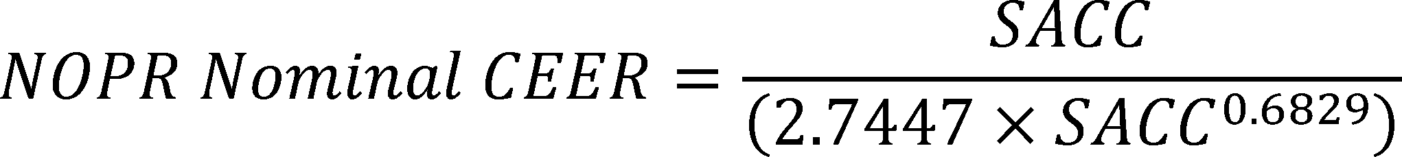
In the June 2016 ECS NOPR, DOE then assessed the relative efficiency of each unit in the test sample by comparing the measured CEER from testing to the nominal CEER as defined by the equation above (DOE will refer to this ratio of actual CEER to nominal CEER as the performance ratio (PR) for a given unit). DOE proposed to define baseline performance as a PR of 0.72, which is based on the minimum PR observed for units in the test sample. Additional details on the baseline units are in chapter 5 of the NOPR TSD.
AHAM objected to the methodology used to determine the baseline level proposed in the June 2016 ECS NOPR, stating that the limited data sample was not representative of the minimum performance of products on the market and that it would have been able to provide test data on a wide range of products if the test procedure had been finalized earlier. Nonetheless, AHAM stated that the combined DOE and newly developed AHAM data set suggests that DOE's proposed baseline level is reasonable. (AHAM, No. 43 at pp. 4, 14)
During the July 2016 STD Public Meeting and in a subsequent request for data and information submitted to DOE on July 21, 2016,[20] AHAM requested the R value and R squared value for the regression curve used to develop the nominal CEER equation in the June 2016 ECS NOPR. (AHAM, Public Meeting Transcript, No. 39 at p. 72) AHAM additionally submitted a supplemental request for data and information on July 27, 2016, in which it requested the raw tested and modeled data used to perform the CEER and SACC calculations for all 24 units in DOE's test sample.[21] DOE provided the R value (0.7420) and R squared value (0.6424) in the DOE response memo, which was accompanied by files containing the requested data for all of DOE's test units. Although AHAM further sought to obtain model numbers for units in the test sample to ascertain how representative DOE's 24 test units were of the U.S. market, DOE identified test units only by sample number in order to maintain confidentiality of the results. (AHAM, No. 43 at pp. 4, 14)
AHAM also expressed concern that DOE did not appear to have run a complete test using the final test procedure and instead relied on a significant amount of modeled data. (AHAM, No. 43 at p. 4) As discussed in the June 2016 ECS NOPR and during the July 2016 STD Public Meeting, all product capacities and efficiencies considered for the June 2016 ECS NOPR analysis were consistent with the appendix CC test procedures. Additionally, modeling was not required to determine the performance of the 18 single-duct portable ACs in DOE's test sample. DOE modeled the performance of the seven dual-duct portable ACs at the lower temperature test condition required in appendix CC.
After the June 2016 ECS NOPR analysis, AHAM compiled additional test data from its members for 22 portable ACs whose results are listed in Table IV.4. (AHAM, No. 43 at pp. 3, 5-6)
| Unit | Configuration | Tested CEER (Btu/Wh) | SACC (Btu/h) | Cooling power (W) | PR |
|---|---|---|---|---|---|
| A | Single-Duct | 5.81 | 6507.57 | 807.75 | 0.91 |
| E | Single-Duct | 5.88 | 6950.00 | 846.00 | 0.90 |
| J | Single-Duct | 6.82 | 8242.83 | 861.75 | 0.98 |
| D | Single-Duct | 4.75 | 4033.24 | 579.71 | 0.90 |
| H | Single-Duct | 4.46 | 4737.80 | 740.13 | 0.79 |
| S | Single-Duct | 6.27 | 7692.11 | 854.25 | 0.92 |
| G | Single-Duct | 6.47 | 8152.20 | 879.26 | 0.93 |
| C | Single-Duct | 5.00 | 5159.80 | 636.00 | 0.86 |
| K | Single-Duct | 5.20 | 6702.80 | 790.50 | 0.81 |
| N | Single-Duct | 5.50 | 8334.20 | 958.50 | 0.78 |
| P | Single-Duct | 6.50 | 9393.00 | 971.25 | 0.88 |
| B | Single-Duct | 6.78 | 6687.50 | 990.00 | 1.05 |
| L | Single-Duct | 5.48 | 3411.44 | 581.10 | 1.11 |
| F | Single-Duct | 5.97 | 4474.20 | 988.90 | 1.09 |
| M | Single-Duct | 5.46 | 6836.43 | 1206.00 | 0.84 |
| R | Single-Duct | 5.01 | 7031.25 | 1238.00 | 0.76 |
| Q | Single-Duct | 4.79 | 6371.60 | 1281.00 | 0.76 |
| O | Single-Duct | 5.21 | 5362.36 | 914.00 | 0.88 |
| T | Single-Duct | 5.63 | 5324.20 | 869.00 | 0.96 |
| W | Single-Duct | 6.35 | 7012.40 | 1031.00 | 0.97 |
| Z | Single-Duct | 6.17 | 8190.80 | 1253.00 | 0.89 |
| U | Single-Duct | 6.28 | 8854.60 | 1312.00 | 0.87 |
AHAM analyzed the combined sample set of its and DOE's data, totaling 47 units, to determine the best-fit power regression, a new nominal CEER equation (shown below), and the relative efficiency of each unit in the combined test sample by comparing the measured CEER from testing to the new nominal CEER. AHAM confirmed DOE's conclusion in the June 2016 ECS NOPR that efficiency would typically increase with capacity, but estimated different coefficients in the nominal CEER equation. (AHAM, No. 43 at pp. 3, 5-6)

In conducting this final rule engineering analysis, DOE included the data supplied by AHAM and also reassessed its own test data and performance modeling. DOE corrected minor errors in its test data and more accurately represented the modeled performance of dual-duct units operating at the lower 83 °F test condition. For those units where the user manual clearly states that the fan operates continuously during off-cycle mode, DOE included the off-cycle mode power in this final rule analysis.
For the final rule, DOE updated the relationship between cooling mode power and SACC and the subsequent nominal CEER equation to reflect the revised set of test and modeled data. The resulting updated nominal CEER equation is shown below.

DOE reassessed the PRs for each unit and found the baseline value to be 0.67, which is the minimum PR observed in the combined test sample. Although this baseline PR value is lower than the value of 0.72 presented in the June 2016 ECS NOPR, applying the new value to the updated nominal CEER curve results in a baseline efficiency level curve for this final rule that closely matches the baseline efficiency level analyzed in the June 2016 ECS NOPR. Additional details on the baseline units efficiency level are included in chapter 5 of the final rule TSD.
b. Higher Energy Efficiency Levels
DOE develops incremental efficiency levels based on the design options manufacturers would likely use to improve portable AC efficiency. While certain technology options identified in Table IV.1 of this final rule and discussed in chapter 3 of the final rule TSD meet all the screening criteria and may produce energy savings in certain real-world situations, DOE did not further consider each of them in the engineering analysis because specific efficiency gains were either not clearly defined or the DOE test procedure would not capture those potential improvements. Such technology options that were not considered are: (1) Adding a subcooler or condenser coil, (2) increasing the heat transfer coefficients, (3) improving duct connections, (4) improving case insulation, (5) implementing part-load technologies, and (6) substituting R-32 for the commonly used R-410A refrigerant. Further discussion of these technology options and the reasons why DOE tentatively concluded that they would be unlikely to be implemented to improve efficiency can be found in chapter 5 of the final rule TSD.
i. June 2016 Standards NOPR Proposal
In the February 2015 Preliminary Analysis, DOE conducted its engineering analysis, including defining efficiency levels, assuming that manufacturers would rely on airflow optimization to improve portable AC efficiencies. However, for the June 2016 ECS NOPR analysis, DOE updated the efficiency levels to reflect performance based on appendix CC, which was different from the proposed test procedure that was the basis of the February 2015 Preliminary Analysis. Appendix CC includes a second cooling mode outdoor test condition for dual-duct units and infiltration air conditions for both single-duct and dual-duct units. The CEER metric for both single-duct and dual-duct units includes a weighted-average measure of performance at the two cooling mode test conditions, along with measures of energy use in standby and off modes. Appendix CC does not include provisions proposed in the February 2015 TP NOPR for measuring case heat transfer.
As discussed in the February 2015 Preliminary Analysis, although the initial test procedure proposal included a CEER metric that combined energy use in cooling mode, heating mode, and various low-power modes, the preliminary analysis was conducted using cooling mode energy efficiency ratio (EERcm) as the basis for energy conservation standards because cooling is the primary function for portable ACs, and DOE expected that manufacturers would likely focus on improving efficiency in this mode to achieve higher CEERs. Because appendix CC does not include a heating mode test and includes a second cooling mode test condition, the CEER metric as codified combines the performance at both cooling mode test conditions with energy use in the low-power modes. Accordingly, DOE utilized CEER as the basis for its proposed portable AC energy conservation standards in the June 2016 ECS NOPR. DOE also based the June 2016 ECS NOPR analysis on the SACC measured in appendix CC, a weighted average of the adjusted cooling capacities at the two cooling mode test conditions.
The two cooling mode test conditions in appendix CC are weighted based on the percentage of annual hours for each test condition, on average, for geographical locations that correspond to expected portable AC ownership. The majority (80 percent) of the total hours were estimated to relate to the lower of the two outdoor temperatures, 83 degrees Fahrenheit (°F) dry-bulb. Because at this lower outdoor temperature, there is only a 3 °F dry-bulb temperature differential and subsequent 0.38 Btu per pounds of dry air enthalpy differential between the indoor and outdoor air, the potential impact of infiltration air heating effects on the overall CEER metric is substantially reduced. For this reason, DOE found no significant relationship between duct configuration or air flow optimization and improved efficiency, and therefore alternatively considered component efficiency improvements as the primary means to increase CEER in the June 2016 ECS NOPR engineering analysis. Accordingly, in the June 2016 ECS NOPR, DOE defined its efficiency levels, other than the max-tech, based on the performance observed in its test sample, independent of duct configuration or level of air flow optimization.
As discussed previously in section IV.C.1.a, in the June 2016 ECS NOPR, DOE characterized and compared performance among all portable ACs in its test sample and determined a relationship between SACC and a general representation of expected CEER. DOE then assessed individual unit performance relative to this nominal CEER relationship and identified a baseline efficiency level at PR = 0.72, with PR defined as the ratio of actual CEER to nominal CEER.
For Efficiency Level 2 (EL 2), DOE determined the PR that corresponded to the maximum available efficiency across a full range of capacities (1.14), and then selected an intermediate Efficiency Level 1 (EL 1) based on a PR between the baseline and EL 2 (0.94). For Efficiency Level 3 (EL 3), DOE identified the PR for the single highest efficiency unit observed in its test sample (1.31).
Due to the variations in performance among units in DOE's test sample, DOE conducted additional performance modeling to augment its test data when estimating efficiency and manufacturing costs at each efficiency level. DOE numerically modeled component improvements for each of the 21 out of 24 test units for which detailed component information were available to estimate potential efficiency improvements to existing product configurations. The component improvements were performed in three steps for each unit.
The first incremental improvement for each unit included a 10-percent increase in heat exchanger frontal area and raising the compressor energy efficiency ratio (EER) to 10.5 Btu/Wh, the maximum compressor efficiency identified at the time of the February 2015 Preliminary Analysis.
The second incremental component efficiency improvement step for each unit included a 15-percent increase in heat exchanger frontal area from the original test unit and an improvement in compressor efficiency to an EER of 11.1 Btu/Wh, which DOE identified as the maximum efficiency for currently available single-speed R-410A rotary compressors of the type typically found in portable ACs and other similar products. As with the 10-percent heat exchanger area increase, DOE expected that a chassis size and weight increase would be necessary to fit a 15-percent increased heat exchanger, but concluded that portability and consumer utility would not be significantly impacted.
DOE included all available design options in the third efficiency improvement step for each unit, including a 20-percent increase in heat exchanger frontal area from the original test unit, more efficient electronically commutated motor (ECM) blower motor(s), and a variable-speed compressor with an EER of 13.7 Btu/Wh. DOE concluded that a 20-percent increase in heat exchanger size was the maximum allowable increase for consumer utility and portability to be retained, as discussed in section IV.B.2 of this document. DOE also improved standby controls efficiency in this final step, adjusting the standby power for each test unit to the minimum observed standby power of 0.46 watts (W) in its test sample. With these design options modeled for units in its test sample, DOE found that the single, theoretical maximum-achievable efficiency among all modeled units corresponded to a PR of 1.75, which DOE defined as Efficiency Level 4 (EL 4).
Table IV.5 summarizes the specific improvements DOE considered when modeling the performance of higher efficiency design options applied to each test unit in the June 2016 ECS NOPR. Depending on the unit, these design options could be associated with different efficiency levels above the baseline.
| Heat exchanger area (% increase) | Compressor EER (Btu/Wh) | Blower motor (type) | Standby (watts) |
|---|---|---|---|
| 10% | 10.5 (single-speed) | (1) | |
| 15% | 11.1 (single-speed) | ||
| 20% | 13.7 (variable-speed) | ECM (variable-speed) | 0.46 |
| 1 No blower motor or standby power changes were applied to the first two incremental steps. | |||
In the June 2016 ECS NOPR, DOE analyzed efficiency levels according to the original nominal CEER equation previously discussed and the PR values listed in Table IV.6:

| Efficiency level | Efficiency level description | Performance ratio (PR) |
|---|---|---|
| Baseline | Minimum Observed | 0.72 |
| EL 1 | Intermediate Level | 0.94 |
| EL 2 | Maximum Available for All Capacities | 1.14 |
| EL 3 | Maximum Observed | 1.31 |
| EL 4 | Max-Tech (Maximum of Modeled Component Improvements) | 1.75 |
Figure IV.1 plots each efficiency level curve for SACCs from 50 to 10,000 Btu/h, based on the June 2016 ECS NOPR nominal CEER curve scaled by the PR assigned to each efficiency level.

Additional details on the selection of efficiency levels in the June 2016 ECS NOPR may be found in chapter 5 of the NOPR TSD.
ii. June 2016 Standards NOPR Comments and Responses
Variable Speed Compressors
ASAP and the Joint Commenters agreed with DOE's consideration of variable-speed compressors in the STD NOPR analysis and agreed that they can improve both part-load and full-load efficiency. (ASAP, Public Meeting Transcript, No. 39 at pp. 72; Joint Commenters, No. 44 at p. 5) The California IOUs supported the inclusion of variable-speed compressors as a technology option and, although DOE was unable to identify any portable AC models that utilize variable-speed compressors, they suggested that DOE consider models, such as the Climax VS12. (California IOUs, No. 42 at p. 2)
AHAM noted that the test procedure proposed at the time of the June 2016 ECS NOPR would not capture any efficiency gains associated with implementing a variable-speed compressor for single-duct units, as there is no part-load requirement for single-duct portable ACs and the test is conducted at one temperature. AHAM therefore suggested that DOE not consider variable-speed compressors for single-duct portable ACs in the engineering analysis. AHAM suggested that the burden and costs of implementing a variable-speed compressor for portable ACs would outweigh the efficiency gains and it would also lead to larger and heavier enclosures (20-percent larger chassis). AHAM also stated that manufacturers would need to use inverter controls that are costly and would also require an electronic expansion valve to modulate refrigerant flow differently as compared to a single-speed compressor, both of which are costly design options. (AHAM, No. 43 at p. 13)
DOE included variable-speed compressors as a design option in the June 2016 ECS NOPR because of their high efficiency during continuous operation, and not for their part-load capability. As discussed in chapter 5 of the June 2016 ECS NOPR TSD, DOE modeled each test unit with a variable-speed compressor with an EER of 13.7 Btu/Wh, representative of the maximum available compressor efficiency for the capacity range appropriate for portable ACs. This EER is consistent with the EER of the compressor used in the Climax VS12 unit identified by the California IOUs. DOE's estimates for efficiency improvements in the June 2016 ECS NOPR were based on the maximum operational efficiency and did not consider part-load efficiency gains. Therefore, DOE's consideration of variable-speed compressors is appropriate for both single-duct and dual-duct portable ACs in this final rule analysis. In addition, DOE's analysis accounted for the higher costs when incorporating variable-speed compressors, including their more costly controls. DOE also modeled larger case sizes that would accommodate larger heat exchangers, and the larger case sizes would also accommodate variable-speed compressors and their associated components.
Improved Compressor Efficiency and Availability
AHAM agreed with DOE's assessment of inertia and scroll compressors, stating that implementing these compressors would significantly affect portability and consumer utility of the product. AHAM noted that a portable AC is used entirely inside a home with no portion of the portable AC located outside, and therefore, noise and vibration may be a concern for a more efficient compressor that would be noisier, larger, and more costly to implement. (AHAM, No. 43 at p. 11)
Consistent with the June 2016 ECS NOPR analysis, DOE did not consider inertia or scroll compressors in developing the final rule efficiency analysis.
AHAM commented that determining the sizes of compressors available in the future for portable ACs may be difficult considering that manufacturers may begin developing compressors for alternative refrigerants. AHAM therefore suggested that DOE determine the future availability of current compressors through discussions with compressor manufacturers. AHAM agreed with DOE's assessment that moving to EL 3 or EL 4 would force manufacturers to remove certain portable AC cooling capacities from the market due to compressor availability being driven by room ACs. (AHAM, No. 43 at pp. 11, 17)
The Joint Commenters suggested that DOE's concerns regarding the availability of high-efficiency compressors to meet higher efficiency levels are unwarranted. They noted that because portable ACs are a newly covered product, the lead time between the publication of the final rule and the compliance date will be 5 years, and therefore, manufacturers and component suppliers, including compressor manufacturers, will have 5 years to develop new products and components. The Joint Commenters further noted that the markets for both room ACs and dehumidifiers will likely drive increased production of high-efficiency compressors, especially because the next room AC standard is scheduled to take effect no later than 2022 and DOE is funding a project conducted by ORNL in partnership with GE to develop a 13 EER room AC. The Joint Commenters also noted that dehumidifiers use similar components as portable ACs and a new ENERGY STAR specification for dehumidifiers that will take effect later this year is likely to drive increased compressor efficiencies. The Joint Commenters asserted that available compressor efficiencies typically increase over time, as seen in the recent room AC rulemaking, and it is therefore reasonable to expect that the available efficiencies of both single-speed and variable-speed compressors will increase in the years before a portable AC standard takes effect. The Joint Commenters concluded that the long lead time before the portable AC standard would take effect, along with multiple market drivers, would ensure adequate availability of high-efficiency compressors to meet higher efficiency levels. (Joint Commenters, No. 44 at pp. 1-3)
DOE conducts its analyses based on currently available information. Accordingly, DOE has analyzed compressor efficiencies for compressors currently available to manufacturers. While the highest efficiency single-speed and variable-speed compressors are available in the appropriate capacity range for portable ACs, the number of models and different capacities available may not be sufficient to cover the entire range of portable AC capacities a manufacturer would include in its product line. The 5-year period prior to compliance with the standards established in this final rule may allow compressor manufacturers sufficient time to develop components and products for a range of efficiencies. However, as stated in the June 2016 ECS NOPR, compressor availability for portable ACs is largely driven by the room AC market. Compressors optimized for room AC operation are not necessarily optimal for portable ACs. Therefore, DOE maintains its concerns regarding availability of the highest efficiency single-speed and variable-speed compressors for portable ACs, and took these concerns into account when establishing the standards in this final rule.
Case Insulation
In chapter 5 of the June 2016 ECS NOPR TSD, DOE concluded that adding insulation to the product case would result in little or no improvement compared to existing product cases. Because heat transfer through the case has a minimal impact on overall cooling capacity, the test procedure adopted in appendix CC does not include a measurement of case heat transfer.
AHAM proposed that because DOE is not aware of any portable ACs that use additional case insulation, it should be removed as a technology option due to the lack of data. AHAM observed that DOE did not include a measure of case heat transfer in the CEER metric in appendix CC because DOE concluded it was insignificant, and therefore any energy savings would not be captured by the test procedure and would have no impact on the standards analysis. (AHAM, No. 43 at p. 12)
DOE identified case insulation as a technology option because it may improve the efficiency of portable ACs when operated in the field, albeit by a small amount. This technology option satisfies all four of the screening analysis criteria, and was therefore retained in the screening analysis and considered in the engineering analysis. However, case insulation was not considered as a means manufacturers would likely use to improve efficiency in the June 2016 ECS NOPR engineering analysis due to its insignificant impact on capacity. DOE adopts that same approach in this final rule.
Improved Duct Connections and Airflow Optimization
In chapter 5 of the June 2016 ECS NOPR TSD, DOE noted that no units in the test sample provided additional sealing in the duct connections. DOE, therefore, lacked information regarding leakage rates and potential savings associated with reducing condenser air leakage to the room, and did not further consider the improvements associated with improved duct connections in the June 2016 ECS NOPR.
The Joint Commenters noted that while DOE was unable to incorporate improved duct connections as a technology option in the June 2016 ECS NOPR engineering analysis due to lack of data, manufacturers may be able to improve duct connections as a way to improve efficiency. (Joint Commenters, No. 44 at p. 4)
AHAM commented that it has no information regarding the heat impacts of air leakage at the duct connections and, based on DOE's own assessment and lack of data, proposed that DOE remove this as a design option. (AHAM, No. 43 at p. 12)
DOE notes that although duct connections were not ultimately implemented to reach higher efficiency levels in the June 2016 ECS NOPR engineering analysis, this technology option satisfies all four of the screening analysis criteria and was therefore retained in the screening analysis and considered in the engineering analysis. DOE adopts that same approach in this final rule.
Improved Standby Controls
In chapter 5 of the June 2016 ECS NOPR TSD, DOE discussed improved standby efficiency as a component improvement in the engineering analysis.
AHAM asserted that there is no substantial gain from improving standby power of electronic controls in terms of improving efficiency and therefore proposed that DOE remove it as a technology option as there will be an insignificant impact when compared to overall portable AC energy consumption. (AHAM, No. 43 at p. 11)
DOE observes that improved standby power would positively impact CEER, and the impact would be measurable, albeit small, under appendix CC. Because appendix CC can quantify the effect of improved standby power and because DOE observed this design option in use in its test sample, DOE considered it in the June 2016 ECS NOPR engineering analysis and in this final rule. Further, DOE notes that EPCA requires that DOE address standby mode and off mode energy use in its energy conservation standards. (42 U.S.C. 6295(gg)(3))
Microchannel Heat Exchangers
In the chapter 5 of the June 2016 ECS NOPR TSD, DOE concluded that because portable ACs already include many design options to improve heat transfer in the evaporator and condenser, and because it lacked information on the potential efficiency gains with microchannel heat exchangers, microchannel heat exchangers were not considered in the engineering analysis as a design option to reach increased portable AC efficiencies. DOE expected that manufacturers would most likely rely on increased heat exchanger cross sectional areas to improve heat transfer and increase efficiencies.
AHAM agreed with DOE and further stated that microchannel heat exchangers do not work well for portable ACs because they are more suitable for the condenser rather than the evaporator due to the difficulty in draining condensing water. AHAM also commented that, because portable ACs spray condensed water onto the condenser to increase the heat exchange, poor draining capability will also affect the condenser. AHAM also asserted that microchannel heat exchangers are complicated, extremely expensive to implement, and easily retain more dirt in the unit, decreasing cooling performance at a much faster rate. (AHAM, No. 43 at pp. 10-11)
ASAP and the Joint Commenters noted that the NOPR engineering analysis did not consider potential efficiency gains from microchannel heat exchangers, which may be utilized by manufacturers to meet the portable AC energy conservation standards. The Joint Commenters referenced research performed in 2006 that found microchannel condensers can result in a 6- to 10-percent increase in refrigeration system efficiency, and additional research for mobile air conditioning that indicated that microchannel heat exchangers can increase efficiency by 8 percent. (ASAP, Public Meeting Transcript, No. 39 at pp. 67-68; Joint Commenters, No. 44 at p. 4)
DOE agrees that microchannel heat exchangers are associated with efficiency improvements, but also agrees with AHAM regarding the complexity of incorporating these heat exchangers into portable ACs. Due to the issues in implementing microchannel heat exchangers and the lack of information regarding their use in portable ACs, DOE maintains the June 2016 ECS NOPR approach for this final rule analysis, in which DOE does not consider this design option in the engineering analysis because it expects that manufacturers would instead rely on increasing heat exchanger cross-sectional areas to increase heat transfer.
Market Distribution
AHAM analyzed the data in the combined sample of portable ACs and concluded that a greater percentage of test units fell short of the proposed efficiency level (TSL 2) than DOE estimated for its own test sample in the June 2016 ECS NOPR. AHAM determined that 17 percent of units in the combined dataset would meet TSL 2, suggesting that 83 percent of the units would require a redesign. Therefore, AHAM proposed that DOE adopt a median PR of 0.90 based on the combined AHAM and DOE data. AHAM stated that a PR of 0.90 would better reflect the current status of units on the market and also would require more reasonable redesigns for manufacturers, especially for a new standard. AHAM noted that its proposed level is between DOE's June 2016 ECS NOPR TSL 1 and TSL 2, and according to AHAM would require a 50-percent redesign of the tested units. (AHAM, No. 43 at pp. 7-8)
As discussed in chapter 5 of the June 2016 ECS NOPR TSD, DOE assessed the number of units that would require a complete product redesign, as opposed to less costly and impactful component improvements, and found that 46 percent of units in the test sample would require a significant product redesign at TSL 2 (see table 5.5.4 in the STD NOPR TSD). Also, DOE's energy conservations standards are not determined solely based on the number of units that would require updates to meet the new levels, but rather the range of criteria discussed in section II.A of this document. These considerations are discussed at length in the June 2016 ECS NOPR and TSD and are reassessed and addressed in this final rule.
As discussed in the following section, DOE considered the combined DOE and AHAM dataset to update its engineering analysis in this final rule.
iii. Final Rule Analysis
For this final rule, DOE maintained the engineering analysis approach utilized in the June 2016 ECS NOPR, with additional modifications and improvements based primarily on comments and data received in response to the June 2016 ECS NOPR. As discussed in in section IV.C.1.a, DOE updated the test data and improved the performance modeling in this final rule and subsequently updated the relationship for nominal CEER based on measured SACC as follows:

DOE also identified a baseline efficiency level with a PR of 0.67 for this final rule, based on the updated test unit performance.
DOE subsequently adjusted its efficiency levels based on the updated unit performance data utilized in this final rule. For EL 2, DOE determined the PR that corresponded to the maximum available efficiency across a full range of capacities (1.04), and then selected an intermediate efficiency level for EL 1 based on a PR between the baseline and EL 2 (0.85). For EL 3, DOE identified the PR for the single highest efficiency unit observed in its test sample (1.18).
In this final rule, DOE relied on the same numerically modeled component improvements for each of the 21 out of 24 test units considered in the June 2016 ECS NOPR. DOE also modeled component improvements for an additional 2 units for which DOE identified detailed component information. The component improvements were performed in three steps for each unit, similar to the improvements conducted for the June 2016 ECS NOPR engineering analysis. For this final rule, DOE utilized the same component efficiency improvements outlined in Table IV.5, maintaining the same maximum single-speed and variable speed compressor efficiencies (11.1 Btu/Wh and 13.7 Btu/Wh, respectively), the same maximum percent heat exchanger frontal area increases (20 percent), the switch from a permanent split capacitor (PSC) motor to an ECM for the blower, and a minimum standby power of 0.46 W.
With these design options modeled for units in its test sample, DOE found that the single, theoretical maximum-achievable efficiency among all modeled units corresponded to a PR of 1.62, which DOE defined as EL 4.
DOE emphasizes that the changes listed in Table IV.5 do not uniquely correlate with efficiency levels beyond the baseline. Baseline through EL 3 are defined by the range of test data, while EL 4 is defined by the maximum theoretical PR after modeling all design options listed in Table IV.5.
In this final rule, DOE analyzed efficiency levels based on test samples and modeled performance according to the following equation and the PR values listed in Table IV.7:

| Efficiency level | Efficiency level description | Performance ratio (PR) |
|---|---|---|
| Baseline | Minimum Observed | 0.67 |
| EL 1 | Intermediate Level | 0.85 |
| EL 2 | Maximum Available for All Capacities | 1.04 |
| EL 3 | Maximum Observed | 1.18 |
| EL 4 | Max-Tech (Maximum of Modeled Component Improvements) | 1.62 |
Figure IV.2 plots each efficiency level curve for SACCs from 50 to 10,000 Btu/h, based on the nominal CEER curve scaled by the PR assigned to each efficiency level.

Additional details on the selection of efficiency levels may be found in chapter 5 of the final rule TSD.
2. Manufacturer Production Cost Estimates
In the February 2015 Preliminary Analysis, DOE developed incremental MPC estimates based on the optimized airflow approach to improving efficiencies. For the June 2016 ECS NOPR analysis, DOE developed new incremental MPC estimates based on the changes to the efficiency levels detailed in section IV.C.1 of the June 2016 ECS NOPR, and also based on feedback from interested parties and on information gathered in additional manufacturer interviews. When assigning costs to efficiency levels in the June 2016 ECS NOPR analysis, DOE considered all units that performed between two efficiency levels as representative of the lower of the two efficiency levels. DOE determined an average baseline MPC based on the units in DOE's test sample with a CEER below EL 1 (PR = 0.94). Six units in the test sample with a market-representative range of capacities tested below EL 1. The average MPC of these six units reflected the baseline MPC for the overall portable AC market.
DOE subsequently determined the costs for all other torn-down and modeled units, and determined the average costs associated with each incremental component efficiency improvement when moving between efficiency levels. In addition to the costs associated with the improved components themselves, DOE also considered the increased costs associated with other related product changes, such as increasing case sizes to accommodate larger heat exchangers.
Although DOE's test and modeled data resulted in a range of PRs from 0.72 to 1.75, DOE noted in the June 2016 ECS NOPR that not all units in its test sample were capable of reaching higher PRs with the identified design option changes. For example, the modeled max-tech PR represented a unit in the test sample that had a high PR as a starting point (near EL 3). Modeling increased heat exchanger sizes and a more efficient compressor in that unit resulted in a higher modeled PR than could be achieved theoretically by applying the same design options to baseline units. For the units that started at lower PRs, DOE expected that manufacturers would have to undertake a complete product redesign and optimization to reach higher PRs, rather than just applying the identified design options. As a result, manufacturers of these units would incur higher MPCs to reach the higher efficiency levels and also significant conversion costs associated with updating their product lines. These conversion costs are discussed further in chapter 12 of the June 2016 ECS NOPR TSD.
In the June 2016 ECS NOPR, DOE found that only three units in the teardown sample would be capable of reaching EL 3 without significant product redesign (i.e., the one unit that tested at EL 3 and two units that could theoretically achieve EL 3 with the highest efficiency single-speed compressors and increasing the heat exchanger area no more than 20 percent). At EL 4 (max-tech), DOE determined all products would require significant product redesigns, as reaching the maximum modeled efficiency would require a 20-percent increase in heat exchanger area and the most efficient variable-speed compressor. DOE noted that manufacturers would likely undertake a product redesign when switching from a single-speed to a variable-speed compressor. Additionally, as discussed in section IV.C.1.b of this document, the ability of a product to reach EL 3 or EL 4 would be dependent on the availability of the most efficient components. However, compressor availability for portable ACs is largely driven by the room AC industry, so the most efficient single-speed and variable-speed compressors may not be available over the entire range of capacities necessary for all portable AC product capacities. As a result, DOE determined that moving to EL 3 or EL 4 may necessitate manufacturers to remove certain portable AC cooling capacities from the market.
For the June 2016 ECS NOPR, DOE calculated all MPCs in 2014 dollars (2014$), the most recent year for which full-year data was available at the time of the analysis. Table IV.8 presents the MPC estimates DOE developed for the June 2016 ECS NOPR.
| Efficiency level | Incremental MPC (2014$) |
|---|---|
| Baseline | |
| EL1 | $29.78 |
| EL2 | 45.13 |
| EL3 | 60.35 |
| EL4 | 108.99 |
Additional details on the development of the incremental cost estimates for the June 2016 ECS NOPR analysis may be found in chapter 5 of the June 2016 ECS NOPR TSD.
During the July 2016 STD Public Meeting, AHAM stated it would work to gather and provide to DOE product cost information. (AHAM, Public Meeting Transcript, No. 39 at p. 75-76) GE commented that it was unable to provide accurate cost feedback due to concerns regarding conducting the test procedure and testing units of all duct configurations. (GE, Public Meeting Transcript, No. 39 at p. 18)
AHAM subsequently stated that it and its members were unable to verify the manufacturer product cost estimates in the June 2016 ECS NOPR because all portable ACs are produced overseas, and the new test procedures will require reductions in reported capacities of existing products. AHAM suggested that manufacturers have not yet fully explored the design requirements to reach the various ELs and therefore urged DOE to reassess its engineering and costing analysis to incorporate the effects of both capacity changes and modifications necessary to meet the ELs. AHAM argued that it is not sufficient to say that the costs associated with the capacity changes are incorporated in all ELs from the base case onward because the constraints on size and portability to maintain the product as portable will have significant effects on the practicality of technology options, particularly adding evaporator or condenser coil area. (AHAM, No. 43 at p. 22)
GREE commented that, based on its calculations, larger chassis designs are necessary to meet the proposed standards and consumers are likely unwilling to accept the additional costs associated with tooling. (GREE, Public Meeting Transcript, No. 39 at pp. 21-22)
As discussed in chapter 5 of the June 2016 ECS NOPR TSD, based on the range of observed heat exchanger areas in its test sample, DOE determined that a 20-percent increase in heat exchanger area is an appropriate limit to maintain portability and avoid impacting consumer utility. DOE also notes that all costs necessary to increase heat exchanger areas and the corresponding chassis design changes were considered in the product cost estimates presented in the June 2016 ECS NOPR and are also considered in this final rule. Additionally, DOE accounted for the changes to both CEER and SACC that would result from incorporating the design option changes in its June 2016 ECS NOPR engineering analysis.
AHAM noted that no portable ACs are manufactured in the U.S., and some are manufactured by third-party manufactures instead of by those who market them. Therefore, AHAM does not believe it is possible to characterize the cost structure of Chinese manufacturing plants and ultimately determine the manufacturer costs for overseas manufacturers. During the July 2016 STD Public Meeting and in its July 21, 2016 request for data and information, AHAM requested insight into how the cost model was developed and how DOE is able to estimate the manufacturing costs for portable ACs. (AHAM, Public Meeting Transcript, No. 39 at pp. 76-77)
The DOE response memo stated that DOE accounts for the location of a manufacturing facility when determining labor costs as well as tooling and equipment costs.[22] Industry financial metrics were estimated using publically available financial information for both manufacturers and importers selling portable ACs in the U.S. DOE also noted that the cost estimates in the June 2016 ECS NOPR accounted for input received from manufacturers and importers during confidential interviews.
For the final rule analysis, DOE followed the same approach as used in the June 2016 ECS NOPR to develop incremental MPC estimates at each efficiency level. DOE updated the incremental MPC estimates from the June 2016 ECS NOPR based on the changes to the ELs detailed in section IV.C.1 of this final rule, feedback from interested parties, improved test unit modeling, and updated cost modeling.
As described in section IV.C.1.a of this final rule, DOE incorporated minor updates to its own data set and included the AHAM test data to determine performance trends and ELs. The adjusted data and slightly different EL curve shape compared to the June 2016 ECS NOPR shifted a few of the data points that would be included in each EL. Additionally, DOE did not have access to the AHAM test units for teardowns or cost modeling, so by necessity relied on its own sample of units to define the representative incremental MPCs at each EL. For this final rule, DOE also calculated all MPCs in 2015$, the most recent year for which full-year data was available at the time of the final rule analysis. Table IV.9 presents the updated MPC estimates DOE developed for this final rule.
| Efficiency level | Incremental MPC (2015$) |
|---|---|
| Baseline | |
| EL1 | $18.95 |
| EL2 | 50.57 |
| EL3 | 93.84 |
| EL4 | 115.53 |
Additional details on the development of the incremental cost estimates for the final rule analysis may be found in chapter 5 of the final rule TSD.
D. Markups Analysis
The markups analysis develops appropriate markups (e.g., manufacturer markups, retailer markups, distributor markups, contractor markups) in the distribution chain and sales taxes to convert the MPC estimates derived in the engineering analysis to consumer prices, which are then used in the LCC and PBP analysis and in the manufacturer impact analysis. At each step in the distribution channel, companies mark up the price of the product to cover business costs and profit margin. For portable ACs, the main parties in the distribution chain are manufacturers, retailers, and consumers.
The manufacturer markup converts MPC to manufacturer selling price (MSP). DOE developed an average manufacturer markup by examining the annual Securities and Exchange Commission (SEC) 10-K reports filed by publicly-traded manufacturers primarily engaged in appliance manufacturing and whose combined product range includes portable ACs.
DOE developed baseline and incremental markups for the manufacturers and retailers in the distribution chain. Baseline markups are applied to the price of products with baseline efficiency, while incremental markups are applied to the difference in price between baseline and higher-efficiency models (the incremental cost increase). The incremental markup is typically less than the baseline markup, and is designed to maintain similar per-unit operating profit before and after new or amended standards.[23]
DOE relied on economic data from the U.S. Census Bureau to estimate average baseline and incremental markups.
AHAM commented that it strongly disagrees with the concept of incremental markups. According to AHAM, manufacturers, wholesalers, retailers and contractors have all provided numerous amounts of data, studies, and surveys saying that the incremental markup concept has no foundation in actual practice. AHAM asked what additional information DOE would need to reassess the markups approach. AHAM further asked if DOE would agree to put the concept of incremental markups up for peer review. (AHAM, No. 39 at pp. 80-81) AHAM states that DOE persists in relying on a simplistic interpretation of economic theory that assumes only variable costs can be passed through to customers because economic returns on capital cannot increase in a competitive marketplace. According to AHAM, they and the other associations and industry participants are unanimous in declaring that DOE's conclusions are simply incorrect and that percentage margins throughout the distribution channels have remained largely constant. In addition, AHAM noted that Shorey Consulting has shown that empirical studies of industry structure and other variables have only weak correlation with profitability, demonstrating that the economic theory DOE relies upon is proven not to apply in practice. Rather than continue to debate past each other, AHAM commented that DOE should submit both its work and that of the various industry groups to an independent peer review process. (AHAM, No. 43 at p. 20)
DOE disagrees that the theory behind the concept of incremental markups has been disproved. The concept is based on a simple notion: An increase in profitability, which is implied by keeping a fixed markup percentage when the product price goes up and demand is relatively inelastic, is not likely to be viable over time in a business that is reasonably competitive. DOE agrees that empirical data on markup practices would be desirable, but such information is closely held and difficult to obtain.
Regarding the Shorey Consulting interviews with appliance retailers, although the retailers said that they maintain the same percentage margin after amended standards for refrigerators took effect, it is not clear to what extent the wholesale prices of refrigerators actually increased. There is some empirical evidence indicating that prices may not always increase following a new standard.[24 25 26] If this happened to be the case following the new refrigerator standard, then there is no reason to suppose that percentage margins changed either.
DOE's analysis necessarily considers a simplified version of the world of appliance retailing; namely, a situation in which other than appliance product offerings, nothing changes in response to amended standards. DOE's analysis assumes that product cost will increase while the other costs remain constant (i.e., no change in labor, material, or operating costs), and asks whether retailers will be able to keep the same markup percentage over time. DOE recognizes that retailers are likely to seek to maintain the same markup percentage on appliances if the price they pay goes up as a result of appliance standards, but DOE contends that over time downward adjustments are likely to occur due to competitive pressures. Some retailers may find that they can gain sales by reducing the markup and maintaining the same per-unit gross profit as they had before the new standard took effect. Additionally, DOE contends that retail pricing is more complicated than a simple percentage margin or markup. Retailers undertake periodic sales and they reduce the prices of older models as new models come out to replace them.[27 28 29] Even if retailers maintain the same percent markup when appliance wholesale prices increase as the result of a standard, retailers may respond to competitive pressures and revert to pre-standard average per-unit profits by holding more frequent sales, discounting products under promotion to a greater extent, or discounting older products more quickly. These factors would counteract the higher percentage markup on average, resulting in much the same effect as a lower percentage markup in terms of the prices consumers actually face on average.
DOE acknowledges that its approach to estimating retailer markup practices after amended standards take effect is an approximation of real-world practices that are both complex and varying with business conditions. However, DOE continues to maintain that its assumption that standards do not facilitate a sustainable increase in profitability is reasonable. Chapter 6 of the final rule TSD provides details on DOE's development of markups for portable ACs.
E. Energy Use Analysis
The purpose of the energy use analysis is to determine the annual energy consumption of portable AC at different efficiencies in representative U.S. single-family homes, multi-family residences, and commercial settings, and to assess the energy savings potential of increased portable AC efficiency. The energy use analysis estimates the range of energy use of portable AC in the field (i.e., as they are actually used by consumers). The energy use analysis provides the basis for other analyses DOE performed, particularly assessments of the energy savings and the savings in consumer operating costs that could result from adoption of amended or new standards.
DOE determined a range of annual energy consumption of portable ACs as a function of the unit's annual operating hours to meet the cooling demand, which depends on the efficiency of the unit, power (watts) of three modes of operation (cooling, fan, and standby), and the percentage of time in each mode. DOE also performed three sensitivity analyses on energy consumption, including looking at the effects of geographical distribution, room threshold size and overall operation time on consumer benefits and costs.
1. Consumer Samples
EIA's Residential Energy Consumption Survey (RECS) provides information on whether households use a room AC. Because portable ACs and room ACs often serve a similar function,[30] DOE developed a sample of households that use room ACs from RECS 2009, which is the latest available RECS.[31] DOE selected the subset of RECS 2009 records that met relevant criteria.[32]
AHAM commented that DOE's consumer sample based on room ACs does not geographically match results AHAM obtained through an online survey. (AHAM, No. 43 at p. 19) Although DOE has not received the full survey results from AHAM, DOE conducted a sensitivity analysis using data points estimated from Figure 6 in Appendix B of AHAM's comments. DOE reweighted its residential and commercial sample such that 24 percent of the sample was from the Northeast, 13 percent from the Midwest, 29 percent from the South, and 34 percent from the West. DOE found that this sensitivity marginally increased LCC savings and reduced the percent of negatively impacted consumers for both sectors. Results for this sensitivity can be found in the final rule TSD appendix 8F.
The California IOUs commented that DOE's estimate for its residential room size threshold of 1,000 square feet could be further refined using data from 2013 study by the National Association of Home Builders. The California IOUs suggested DOE's current method limits the sample of potential installations of portable ACs. (California IOUs, No. 42 at p. 4)
Sizing charts provided by vendors indicate that portable ACs are intended to cool rooms having an area as large as approximately 525 to 600 square feet. A review of retail websites, however, indicated portable ACs may be used in rooms as large as 1,000 square feet. DOE assumed 1,000 square feet to be the maximum room size a user would attempt to cool using a portable AC. In practice, only 60 records in the RECS 2009 sample (about 2 percent) represent rooms between 600 and 1,000 square feet.
As a sensitivity, DOE removed the room size threshold from its analysis and calculated LCC results using the full room AC sample. Removing this threshold made minimal impact on the results. In this scenario, the average LCC savings for residential consumers under the proposed standard (TSL 2) would be $107 (compared with $108 in the primary estimate), and 28 percent of consumers would be impacted negatively (compared with 27 percent in the primary estimate). The simple payback period would be 2.8 years (compared with 2.8 years in the primary estimate). The full sensitivity results can be found in the final rule TSD appendix 8F.
To estimate the operating hours of portable ACs used in commercial settings, DOE developed a building sample from the 2012 Commercial Buildings Energy Consumption Survey (CBECS),[33] again using the operating hours of room ACs as a proxy. DOE used the 2003 CBECS in the June 2016 ECS NOPR analysis. The method is described in chapter 7 of the final rule TSD.
AHAM and the California IOUs encouraged DOE to replace 2003 CBECS data with 2012 CBECS data. (AHAM, No. 39 at pp. 85-87; California IOUs, No. 42 at p. 4)
DOE updates its inputs for analyses with credible and verifiable sources as data become available. At the time the June 2016 ECS NOPR analysis was completed, 2012 CBECS with expenditure microdata was not yet available, so DOE used 2003 CBECS. Because the data set was released in time for use in the final rule, DOE is using 2012 CBECS in its final rule analysis as recommended by AHAM and the California IOUs.
2. Cooling Mode Hours and Sensitivity Analyses
To estimate the cooling operating hours of portable ACs using datasets that are statistically representative, DOE used the same method and updated datasets that were used in the 2011 direct final rule for room ACs. 76 FR 22454 (Apr. 21, 2011). For each sample household, RECS provides the estimated energy use for cooling by room ACs. After assigning an efficiency and capacity to the room AC, DOE could then estimate its operating hours in cooling mode. DOE adjusted the operating hours in cooling mode to account for the likelihood that improvement in building shell efficiency would reduce the cooling load and operating hours.[34] The estimated average of cooling operating hours for a room AC is 612 hours/year.
Some interested parties objected to DOE's use of room AC data as a proxy for portable AC operating hours. AHAM stated that DOE misrepresents portable ACs by referencing and scaling characteristic and performance data from room air conditioners. (AHAM, No. 43 at p. 18) AHAM asserted that for a standards rule to be technologically feasible and economically justified, it must be based on product-specific data, not assumptions and estimates. (AHAM, No. 43 at pp. 1-2) De' Longhi stated that from their experience, while room ACs are typically used as the main cooling system, portable ACs are often used as supplementary systems when central systems are not activated or out of order so that the annual hours of use for portable ACs are lower than for room ACs. (De' Longhi, No. 41 at p. 1)
AHAM and De' Longhi stated that a De' Longhi survey [35] cannot be used to conclude that portable ACs and room ACs have similar cooling mode annual operating hours. De' Longhi asserted that although both portable ACs and room ACs are used in similar periods of the day, that does not mean that they are used for the same number of hours in a day and for the same number of days in a year. They believed that DOE mischaracterized the study and drew conclusions that are not justified from the data. De' Longhi stated that the annual hours of use for portable ACs are on average sensibly lower than for room ACs. (AHAM, No. 43 at pp. 18-19; De' Longhi, No. 41 at p. 2)
DOE maintains that room AC cooling hours are an appropriate proxy for portable AC cooling hours as both products are used for cooling defined spaces and their product usage is broadly similar. However, DOE agrees with the commenters that the De' Longhi survey cannot be used to conclusively draw a relationship between the total annual cooling mode hours of portable ACs and room ACs. To account for potential differences between consumer use of portable ACs and room ACs, DOE conducted a sensitivity analysis which assumes lower annual hours of use for portable ACs in comparison to room ACs. Specifically, in this sensitivity analysis, DOE scaled the room AC cooling mode hours of use by half while maintaining the assumption that portable ACs are used during the same time of year as room ACs, since the use of both types of cooling equipment is likely to be consistent seasonally. The results of this sensitivity analysis estimate one-third of the energy cost savings relative to the primary estimate. In this low-usage case, the average LCC savings under the adopted standards (TSL 2) would be $35 (compared with $125 in the primary estimate), and 42 percent of consumers would be impacted negatively (compared with 27 percent in the primary estimate). The simple payback period would be 5.1 years (compared with 2.8 years in the primary estimate). Further details are presented in appendix 8F and appendix 10E of the final rule TSD. Thus, even if consumers use portable ACs substantially less than room ACs, the overall impacts on consumers would be positive. It should be noted that lower product usage would imply a longer lifetime; however, in this sensitivity analysis, the lifetime was not lengthened. A longer lifetime would increase savings, reduce the payback period, and reduce the population segment that is negatively impacted.
AHAM recommended that DOE use data from the study by Burke et al. to calculate operating hours.[36] (AHAM, No. 43 at p. 20) DOE believes that it would be inaccurate to use the Burke et al. study for estimating operating hours for the nation. As stated in the report itself, given the limited number of test sites in two locations in the Northeast, the Burke et al. study was not intended to be statistically representative of portable AC users in the U.S. It should also be noted that the annual energy use estimates presented in the study are based on metered average outdoor temperatures which were reportedly lower than usual for most summers. In addition, the metering period began in July and it is likely that portable AC owners either in warmer years or in other areas of the country may operate the units in earlier months (May and June), which would contribute to higher annual use. DOE did use the Burke et al. study for estimations of the fan-only mode operation since the report provided the only publicly available fan-only information for any cooling product.
AHAM claims that the data DOE has used raise serious and separate concerns under the Data Quality Act.[37] (Public Law 106-554) According to AHAM, the law and the Office of Management and Budget (OMB) guidelines require agency actions aimed at “maximizing the quality, objectivity, utility, and integrity of information (including statistical information) disseminated by the agency.” Id. at § 515(b)(2)(A). (AHAM, No. 43 at p. 20)
DOE maintains that the data sources and methodology used in its analyses meet the guidelines developed by OMB in response to the Data Quality Act. Data used in DOE's analysis draws from the best available statistically-significant representation of how U.S. consumers use cooling devices similar in function and cooling capacity to portable ACs. Interested parties have been provided opportunities at the preliminary analysis and NOPR stages to make data available to refine DOE's analysis. When reviewed and verified, DOE has incorporated data from comments into its analysis. For example, DOE incorporated analysis data and information from interested parties regarding historical shipments, and product efficiencies and capacities into the final rule. Additionally, DOE performed sensitivity analyses for inputs that are subject to uncertainty to assess the impact of alternative assumptions and reports those results in the final rule TSD.
The California IOUs suggested that DOE use projected cooling degree-days for the LCC analysis year (2022) to accurately quantify the required cooling load. (California IOUs, No. 42 at p. 4) DOE agrees and has incorporated this suggestion into its final rule analysis using census division cooling degree-day trends from AEO 2016.[38] Including cooling degree-day trends increases operating hours by approximately 4 percent. DOE also used the projected change in building shell efficiencies from AEO 2016 when calculating operating hours to account for increased building shell efficiency of the stock.
3. Fan-Only Mode and Standby Mode Hours
To estimate the number of hours in fan-only mode, DOE utilized a field metering analysis of a sample of portable ACs in 19 homes.[39] The survey provided data on cooling-mode and fan-only mode hours of operation. DOE derived a distribution of the ratio of fan-only mode hours to cooling-mode hours, and used this distribution to randomly assign a ratio to each of the sample households, which allows estimation of fan-only mode hours of operation. DOE assumed portable ACs would only be plugged in during months with 5 or more cooling degree days. The annual hours in standby mode were derived by subtracting the cooling-mode and fan-only mode hours of operation from the total number of hours in a months with 5 or more cooling degree days.
Chapter 7 of the final rule TSD provides details on DOE's energy use analysis for portable ACs.
F. Life-Cycle Cost and Payback Period Analysis
DOE conducted LCC and PBP analyses to evaluate the economic impacts on individual consumers of potential energy conservation standards for portable ACs. The effect of new or amended energy conservation standards on individual consumers usually involves a reduction in operating cost and an increase in purchase cost. DOE used the following two metrics to measure consumer impacts:
- The LCC (life-cycle cost) is the total consumer expense of a product over the life of that product, consisting of total installed cost (manufacturer selling price, distribution chain markups, sales tax, and installation costs) plus operating costs (expenses for energy use, maintenance, and repair). To compute the operating costs, DOE discounts future operating costs to the time of purchase and sums them over the lifetime of the product.
- The simple PBP (payback period) is the estimated amount of time (in years) it takes consumers to recover the increased purchase cost (including installation) of a more-efficient product through lower operating costs. DOE calculates the simple PBP by dividing the change in purchase cost at higher ELs by the change in annual operating cost for the year that new standards are assumed to take effect.
For any given EL, DOE calculates the LCC savings as the change in LCC in a standards case relative to the LCC in the no-new-standards case, which reflects the estimated efficiency distribution of portable ACs in the absence of new or amended energy conservation standards. In contrast, the simple PBP for a given EL is measured relative to the baseline product.
For each considered EL, DOE calculated the LCC and PBP for a nationally representative set of housing units and commercial buildings that use portable ACs. DOE used the EIA's 2009 RECS to develop household samples for portable ACs based on households that use room ACs. DOE also used the EIA's 2012 CBECS to develop a sample of commercial buildings that use portable ACs, again based on buildings that use room ACs. For each sample household or commercial building, DOE determined the energy consumption for the portable ACs and the appropriate electricity price. By developing a representative sample of households, the analysis captured the variability in energy consumption and energy prices associated with the use of portable ACs.
Inputs to the calculation of total installed cost include the cost of the product—which includes MPCs, manufacturer markups, retailer and distributor markups, and sales taxes—and installation costs. Note in the case of portable ACs, DOE assumed that installation costs would not change with efficiency ELs. So the difference of installation cost between the baseline and higher ELs is then $0. Inputs to the calculation of operating expenses include annual energy consumption, energy prices and price projections, repair and maintenance costs, product lifetimes, and discount rates. DOE created distributions of values for product lifetime and discount rates with probabilities attached to each value, to account for their uncertainty and variability. Sales tax and electricity prices are tied to the geographic locations of purchasers drawn from the residential and commercial samples.
The model DOE uses to calculate the LCC and PBP relies on a Monte Carlo simulation to incorporate uncertainty and variability into the analysis. The Monte Carlo simulation randomly samples input values from the probability distributions and portable AC user samples. The model calculated the LCC and PBP for products at each EL for 10,000 housing units or commercial buildings per simulation run.
DOE calculated the LCC and PBP for all consumers as if each were to purchase a new product in the expected year of compliance with new standards. Any new standards would apply to portable ACs manufactured 5 years after publication of the final standard. (42 U.S.C. 6295(l)(2)) Therefore, for purposes of its analysis, DOE used 2022 as the first year of compliance with new standards.
Table IV.10 summarizes the approach and data DOE used to derive inputs to the LCC and PBP calculations. The subsections that follow provide further discussion. For energy use, RECS and CBECS were used for number of hours of use in cooling mode. A field metering report provided information regarding the fan-mode of portable ACs.[40] Details of the spreadsheet model, and of all the inputs to the LCC and PBP analyses, are contained in chapter 8 of the final rule TSD and its appendices.
| Inputs | Source/method |
|---|---|
| Product Cost | Derived by multiplying MPCs by manufacturer and retailer markups and sales tax, as appropriate. Producer Price Index (PPI) series for small household electronics fit to an exponential model. |
| Installation Costs | Assumed no installation costs with baseline unit and no cost with EL. |
| Annual Energy Use | Power in each mode multiplied by the hours per year in each mode. Average number of hours based on 2009 RECS, 2012 CBECS, and field metering data. Variability: Based on the 2009 RECS and 2012 CBECS. |
| Energy Prices | Electricity: Based on 2014 average and marginal electricity price data from the Edison Electric Institute. Variability: Marginal electricity prices vary by season, U.S. region, and baseline electricity consumption level. |
| Energy Price Trends | Based on AEO 2016 No-CPP case price projections. Trends are dependent on sector and census division. |
| Repair and Maintenance Costs | Assumed no change with EL. |
| Product Lifetime | Weibull distribution using parameters from room ACs. |
| Discount Rates | Approach involves identifying all possible debt or asset classes that might be used to purchase the considered appliances, or might be affected indirectly. Primary data source was the Federal Reserve Board's Survey of Consumer Finances. |
| Compliance Date | 2022. |
| * References for the data sources mentioned in this table are provided in the sections following the table or in chapter 8 of the final rule TSD. | |
1. Product Cost
To calculate consumer product costs, DOE multiplied the MPCs developed in the engineering analysis by the markups described in section IV.D of this document (along with sales taxes). DOE used different markups for baseline products and higher-efficiency products, because DOE applies an incremental markup to the increase in MSP associated with higher-efficiency products.
Economic literature and historical data suggest that the real costs of many products may trend downward over time according to “learning” or “experience” curves. Experience curve analysis implicitly includes factors such as efficiencies in labor, capital investment, automation, materials prices, distribution, and economies of scale at an industry-wide level.[41] DOE used the most representative Producer Price Index (PPI) series for portable ACs to fit to an exponential model to develop an experience curve. DOE obtained historical PPI data for “small electric household appliances, except fans” from the Labor Department's Bureau of Labor Statistics (BLS) for 1983 to 2015.[42] Although this PPI series encompasses more than portable ACs, no PPI data specific to portable ACs were available. The PPI data reflect nominal prices, adjusted for changes in product quality. DOE calculated an inflation-adjusted (deflated) price index by dividing the PPI series by the Gross Domestic Product Chained Price Index.
2. Installation Cost
Installation cost includes labor, overhead, and any miscellaneous materials and parts needed to install the product. Available evidence indicated that no installation costs would be incurred for baseline installation or be impacted with increased ELs.
3. Annual Energy Consumption
For each sampled household and building, DOE determined the energy consumption for a portable AC at different ELs using the approach described in section IV.E of this final rule.
4. Energy Prices
DOE used average prices (for baseline products) and marginal prices (for higher-efficiency products) which vary by season, region, and baseline electricity consumption level for the LCC. DOE estimated these prices using data published with the Edison Electric Institute (EEI) Typical Bills and Average Rates reports for summer and winter 2014.[43] For the residential sector each report provides, for most of the major IOUs in the country, the total bill assuming household consumption levels of 500, 750, and 1,000 kWh for the billing period. For the commercial sector the report provides typical bills for several combinations of monthly electricity peak demand and total consumption.
For both the residential and commercial sectors, DOE defined the average price as the ratio of the total bill to the total electricity consumption. For the residential sector, DOE used the EEI data to also define a marginal price as the ratio of the change in the bill to the change in energy consumption. For the commercial sector, marginal prices cannot be estimated directly from the EEI data, so DOE used a different approach, as described in chapter 8 of the final rule TSD.
Regionally weighted-average values for each type of price were calculated for the nine census divisions and four large states (CA, FL, NY and TX). Each EEI utility in a division was assigned a weight based on the number of consumers it serves. Consumer counts were taken from the most recent EIA Form 861 data (2012).[44] DOE adjusted these regional weighted-average prices to account for systematic differences between IOUs and publicly-owned utilities, as the latter are not included in the EEI data set.
DOE assigned seasonal average and marginal prices to each household or commercial building in the LCC sample based on its location and its baseline monthly electricity consumption for an average summer or winter month. For a detailed discussion of the development of electricity prices, see appendix 8C of the final rule TSD.
To estimate future prices, DOE used the projected annual changes in average residential and commercial electricity prices that are consistent with cases described on p. E-8 in AEO 2016.[45] AEO 2016 has an end year of 2040. The AEO price trends do not distinguish between marginal and average prices, so DOE used the same trends for both. DOE reviewed the EEI data for the years 2007 to 2014 and determined that there is no systematic difference in the trends for marginal vs. average prices in the data.
5. Maintenance and Repair Costs
Repair costs are associated with repairing or replacing product components that have failed in an appliance. Maintenance costs are associated with maintaining the operation of the product. Based on available data and low product purchase prices, DOE concluded that repair frequencies are low and do not increase for higher-capacity or higher-efficiency units. DOE assumed a zero cost for all ELs.
AHAM commented that higher ELs may require use of variable-speed compressors to meet a potential standard and this would impact the repair rate and cost of higher ELs. (AHAM, No. 43 at pp. 25-26) AHAM was unable to provide data to show that variable-speed compressors would require an increased repair rate or cost, but suggested DOE consult with manufacturers. DOE has not found any evidence that repair rates or costs would increase with efficiency for portable ACs nor did any manufacturer provide data to suggest this occurs in the market today. Therefore, DOE estimates that portable AC repair rates and costs do not change with higher efficiency units.
6. Product Lifetime
The product lifetime is the age at which the product is retired from service. Given similar mechanical components and uses, DOE considered that the lifetime distribution of portable ACs is the same as that of room ACs, as estimated for the 2011 direct final rule. 76 FR 22454 (April 21, 2011). The average lifetime is 10.5 years.
AHAM also noted that although room ACs and portable ACs are used for similar purposes, they are different products and therefore they may have different lifetimes. (AHAM, No. 39 at p. 96) AHAM commented that DOE should use an average product lifetime of 7 years for portable ACs and referenced a 2010 survey conducted by AHAM. (AHAM, No. 43 at pp. 23-24)
AHAM did not provide the survey in its comments and DOE is unable to locate a copy of the survey in the public record; therefore, DOE is unable to verify AHAM's estimate and determine whether the lifetime estimate is specifically for portable ACs or for a similar product. Additionally, if AHAM's estimate is for the portable AC product, it is unclear how a 2010 survey could accurately measure the average lifetime for a product that has only been available in large residential markets since the early 2000s. An accurate calculation of the average lifetime requires at least one full turnover of stock to sample the entire age distribution to include the longest living units that exceed the average lifetime. Assuming the first appreciable number of shipments of portable ACs occurred in 2000, the oldest possible lifetime captured in AHAM's survey would be 10 years. Excluding longer lived portable ACs that have not yet failed would bias an estimate of the average to lower values. Without the details of the survey methodology, DOE is unable to include AHAM's estimate in derivation of a lifetime distribution.
ASAP stated that using the lifetime of room ACs or dehumidifiers is reasonable, given the similarities of the products and the components that make up those products. (ASAP, No. 39 at pp. 98-99) The Joint Commenters noted that portable dehumidifiers are very similar to portable ACs, as the two products share the same basic refrigeration system components and are both portable units placed inside a room. The Joint Commenters also noted that DOE estimates the average lifetime of a portable dehumidifier (11 years) is slightly longer than the average lifetime of a room AC (10.5 years) and therefore, DOE's assumption for the average lifetime of portable ACs may be conservative. (Joint Commenters, No. 44 at p. 6) DOE continues to use an average lifetime of 10.5 years derived from room ACs given the similarity in their components.
Chapter 8 of the final rule TSD provides details on DOE's development of lifetimes for portable ACs.
7. Discount Rates
In the calculation of LCC, DOE applies discount rates appropriate to households to estimate the present value of future operating costs. DOE estimated a distribution of residential discount rates for portable ACs based on consumer financing costs and the opportunity cost of consumer funds.
DOE applies weighted average discount rates calculated from consumer debt and asset data, rather than marginal or implicit discount rates.[46] DOE notes that the LCC does not analyze the appliance purchase decision, so the implicit discount rate is not relevant in this model. The LCC estimates NPV over the lifetime of the product, so the appropriate discount rate will reflect the general opportunity cost of household funds, taking this time scale into account. Given the long time horizon modeled in the LCC, the application of a marginal interest rate associated with an initial source of funds is inaccurate. Regardless of the method of purchase, consumers are expected to continue to rebalance their debt and asset holdings over the LCC analysis period, based on the restrictions consumers face in their debt payment requirements and the relative size of the interest rates available on debts and assets. DOE estimates the aggregate impact of this rebalancing using the historical distribution of debts and assets.
To establish residential discount rates for the LCC analysis, DOE identified all relevant household debt or asset classes in order to approximate a consumer's opportunity cost of funds related to appliance energy cost savings. DOE estimated the average percentage shares of the various types of debt and equity by household income group using data from the Federal Reserve Board's Survey of Consumer Finances [47] (SCF) for 1995, 1998, 2001, 2004, 2007, 2010, and 2013. Using the SCF and other sources, DOE developed a distribution of rates for each type of debt and asset by income group to represent the rates that may apply in the year in which new or amended standards would take effect. DOE assigned each sample household a specific discount rate drawn from one of the distributions. The average rate across all types of household debt and equity and income groups, weighted by the shares of each type, is 4.5 percent. See chapter 8 of the final rule TSD for further details on the development of consumer discount rates.
To establish commercial discount rates for the LCC analysis, DOE estimated the cost of capital for companies that purchase a portable AC. The weighted average cost of capital is commonly used to estimate the present value of cash flows to be derived from a typical company project or investment. Most companies use both debt and equity capital to fund investments, so their cost of capital is the weighted average of the cost to the firm of equity and debt financing as estimated from financial data for publicly traded firms in the sectors that purchase computers. For this analysis, DOE used Damadoran Online [48] as the source of information about company debt and equity financing. The average rate across all types of companies, weighted by the shares of each type, is 5.6 percent. See chapter 8 of the NOPR TSD for further details on the development of commercial discount rates.
AHAM commented that DOE has traditionally used a real (inflation adjusted) discount rate in the LCC calculation based on averaging the various components of debt and assets. AHAM noted that AHAM and others have commented that an average consumer discount rate is inappropriate and that DOE should use a marginal rate based on the cost of available borrowed funds, generally credit card debt. (AHAM, No. 43 at p. 24) In response to questions by AHAM, DOE stated in the DOE response memo and maintains that when assessing the NPV of an investment in energy efficiency, the marginal interest rate alone (assuming it were the interest rate on the credit card used to make the purchase, for example) would only be the relevant discount rate if either: (1) The consumer were restricted from rebalancing their debt and asset holdings (by redistributing debt and assets based on the relative interest rates available) over the entire time period modeled in the LCC analysis; or (2) the risk associated with an investment in energy efficiency was at a level commensurate with that reflected by credit card interest rates (i.e., that the risk premium required for an investment in energy efficiency was very high).[49]
In reference to the first point, rebalancing, AHAM commented that the inherent assumption allowing rebalancing is that consumers will defer consumption (i.e., save) in order to generate surplus cash which can then be used to pay down debt. AHAM stated that this assumption is essential since consumers have no other source of investment capital other than savings (e.g., individuals cannot sell “equity” in themselves). In this case, AHAM suggested that the appropriate discount rate would be the implied rate of return for deferring consumption. AHAM noted that academic studies on implicit discount rates for the consumption/savings tradeoff yield discount rates substantially higher than either the 4.43 percent assumed by DOE or the 11.6 percent recommended by AHAM.[50] AHAM noted that it would be pleased if DOE adopted a consumer discount rate based on the consumption/savings tradeoff. (AHAM, No. 43 at pp. 24-25)
DOE believes that using an average discount rate in the LCC best approximates the actual opportunity cost of funds faced by consumers. This opportunity cost of funds is the time-value of money for consumers. Interest rates, which are set by supply and demand for credit and capital in the financial market, vary across consumers and across financial investment or credit source based on the risk associated with that consumer or with that investment type. Because the purpose of the LCC analysis is to determine the distributional impacts of the proposed standard across heterogeneous consumers in the population, to account for variation in access to rates of return on investments and interest rates of debt faced by consumers in the population, DOE generates a discount rates based on the average of the interest rates associated with debts and assets holdings, weighted by the share of funds associates with each of those debts or assets in the portfolio. This is the best approximation of the actual opportunity cost of funds for each household,[51] and it is the value of deferred consumption as determined by the equilibrium of supply and demand in the financial market. Those with very high rates of discounting for deferred consumption will hold more debt, potentially at higher rates of interest. Those with lower rates will hold less. This is captured in the weighted average calculation of the discount rate used by DOE. Additionally, DOE disagrees with the statement that consumers have no other source of investment capital other than savings. A range of assets is included in the weighted average discount rate calculated by DOE precisely because that is the equity that consumers may hold. In particular, they can either defer putting additional funds towards one of these investments or they can extract equity from one of these investments if they are able. These financial assets are a part of the opportunity cost of funds held by consumers, and that is why they are in the weighted average calculation for the discount rate use by DOE.
In reference to the second point concerning risk, AHAM stated DOE is carrying the concepts of capital asset pricing (CAPM) used in the commercial sector (and used by DOE to set commercial discount rates), which, essentially, assumes that the cost of equity is set in relationship to a risk free rate and the systemic variance between a security (or set of cash flows) and a widely diversified set of equities. AHAM commented that DOE, in discussing point (2), focuses on “risk premiums” associated with types of investments. Within the context of the CAPM model, AHAM stated that all the risks discussed by DOE are diversifiable, non-systemic risk. AHAM suggested that they should be incorporated (and are incorporated by the DOE Monte Carlo process) in the cash flow assessment. AHAM commented that this whole discussion on point (2) is irrelevant to a discussion of appropriate discount rates. (AHAM, No. 43 at p. 25)
First, DOE raised the issue of risk not in the context of its method but rather to explain circumstances in which a higher discount rate might be appropriate. In any case, DOE disagrees that the discussion regarding the risk premium appropriate for an investment in energy efficiency is irrelevant to the choice of discount rate used in the LCC. As DOE stated before, while there is limited data available on the risk associated with specific types of energy efficiency investments, Mills et al. (2006) present results from an analysis demonstrating that the risk associated with the returns from investing in an ENERGY STAR Building are in line with that of long-term government bonds (i.e., quite low). These results are shown in Figure IV.3, below. This is suggestive that there is no reason to assume that the risk premium required for an investment in energy efficiency should be particularly high, and certainly not high enough to justify a required rate of return at a level commensurate with a credit card interest rate.

AHAM stated that the actual question would be what discount rate consumers use to evaluate investments and should that discount rate be some theoretical value (consumers “ought” to look at investments in some manner) or a factual value. AHAM commented that the factual value, or imputed, discount rate for energy or any other investment is substantially greater than four percent, inflation adjusted. AHAM concluded that DOE should either use the short-term marginal cost of funds for consumers, the actual rate used to finance most significant purchases, or it should use a rate to reflect the time value in deferring consumption in the consumption versus saving tradeoff. AHAM noted that either rate is substantially higher than the 4.43 percent used by DOE. (AHAM, No. 43 at p. 25)
As DOE has responded in the past to comments on this topic, the LCC analysis is not modeling a purchase decision. The LCC analysis estimates the NPV of financial trade-offs of increased upfront product costs weighed against reduced operating costs over the lifetime of the covered product, assuming the product has already been obtained and installed. Implicit or “imputed” discount rates referred to by AHAM are not the appropriate rates to use in the context of the LCC analysis because such rates deviate from market interest rates due to a variety of factors (e.g., imperfect information, option values, transaction costs, cognitive biases such as present-based preferences or loss aversion, etc.). All of these factors are irrelevant from the perspective of the LCC analysis; they are already sunk costs. The short-term marginal rate is not the appropriate discount rate to use because fixing the discount rate at the marginal rate associated with a credit card assumes that consumers purchase the appliance with a credit card, and keep that purchase on the credit card throughout the entire time it takes to pay off that debt with only operating costs savings from the more efficient product. There is little evidence that consumers behave in this way.
8. Energy Efficiency Distribution in the No-New-Standards Case
To accurately estimate the share of consumers that would be affected by a potential energy conservation standard at a particular EL, DOE's LCC analysis considered the projected distribution (market shares) of product efficiencies under the no-new-standards case (i.e., the case without new energy conservation standards).
To estimate the energy efficiency distribution of portable ACs for 2022, DOE's LCC analysis considered the projected distribution (market shares) of product efficiencies under the no-new-standards case (i.e., the case without new energy conservation standards). Based on the engineering analysis, DOE found that gains in efficiency were achieved by utilizing more efficient components in existing test units. DOE used product component characteristics to estimate the current efficiency distribution of portable ACs on the market. DOE based EL 1, EL2, and EL 3 on the performance observed in its test sample used to develop the engineering analysis. Therefore, DOE estimated a share of 37 percent at the baseline, 48 percent for EL 1, 13 percent for EL 2, 2.2 percent for EL 3, and no share at EL 4. EL 4 represents the maximum theoretical performance based on modeling the max-tech design options. The estimated market shares for the no-new-standards case for portable ACs and the average EER and CEER values for each EL are shown in Table IV.11. See chapter 8 of the final rule TSD for further information on the derivation of the efficiency distributions.
| Efficiency level | EER | CEER | Market share (%) |
|---|---|---|---|
| Baseline | 5.35 | 5.08 | 37 |
| 1 | 6.05 | 5.94 | 47.8 |
| 2 | 7.15 | 7.13 | 13 |
| 3 | 8.48 | 8.46 | 2.2 |
| 4 | 10.75 | 10.73 | 0 |
9. Payback Period Analysis
The simple PBP is the amount of time it takes the consumer to recover the additional installed cost of more-efficient products, compared to baseline products, through energy cost savings. PBPs are expressed in years. PBPs that exceed the life of the product mean that the increased total installed cost is not recovered in reduced operating expenses.
The inputs to the simple PBP calculation for each EL are the change in total installed cost of the product and the change in the first-year annual operating expenditures relative to the baseline. The PBP calculation uses the same inputs as the LCC analysis, except that discount rates are not applied.
As noted above, EPCA, as amended, establishes a rebuttable presumption that a standard is economically justified if the Secretary finds that the additional cost to the consumer of purchasing a product complying with an energy conservation standard level will be less than three times the value of the first year's energy savings resulting from the standard, as calculated under the applicable test procedure. (42 U.S.C. 6295(o)(2)(B)(iii)) For each considered EL, DOE determined the value of the first year's energy savings by calculating the energy savings in accordance with the applicable DOE test procedure, and multiplying those savings by the average energy price projection for the year in which compliance with the new standards would be required (see section V.B.1.c of this final rule).
G. Shipments Analysis
DOE uses projections of annual product shipments to calculate the national impacts of potential amended or new energy conservation standards on energy use, NPV, and future manufacturer cash flows.[53] The shipments model takes an accounting approach, tracking market shares of each product class and the vintage of units in the stock. Stock accounting uses product shipments as inputs to estimate the age distribution of in-service product stocks for all years. The age distribution of in-service product stocks is a key input to calculations of both the NES and NPV, because operating costs for any year depend on the age distribution of the stock.
DOE received data on portable AC shipments in 2014 from manufacturer interviews. The manufacturer interviews also provided information which suggested that the average annual growth in portable AC shipments between 2004 and 2013 was 30 percent. To estimate historical shipments prior to 2004, DOE interpolated between 1985 (the date that portable ACs were introduced to the residential market) and 2004.
DOE estimated a saturation rate to project shipments of portable ACs. DOE assumed that the portable AC saturation rate would be no greater than half the current room AC saturation rate (based on RECS 2009) by the end of the analysis period, i.e., 2051. For each year of the projection period, the saturation rate of portable ACs was determined from a combination of the total stock of the product and total housing stock. The total stock of portable ACs was based on product lifetime and the survival function developed in the LCC analysis. DOE used total housing stock from AEO 2016. Based on this revised approach, DOE estimated that the shipments of portable ACs would increase from 1.32 million in 2014 to 1.67 million in 2051.
For the final rule analysis, DOE applied price and efficiency elasticity parameters to estimate the effect of new standards on portable AC shipments. DOE estimated the price and efficiency elasticity parameters from a regression analysis that incorporated shipments, purchase price, and efficiency data specific to several residential appliances during 1989-2009. Based on evidence that the price elasticity of demand is significantly different over the short run and long run for other consumer goods (i.e., automobiles), DOE assumed that these elasticities decline over time. DOE estimated shipments in each standards case using the price and efficiency elasticity along with the change in the product price and operating costs between a standards case and the no-new-standards case.
AHAM commented that it believes that DOE has under-estimated the price/feature elasticity effects on portable ACs. AHAM stated that DOE has used a generic elasticity factor without looking at the specific conditions of the portable AC marketplace and that importers who purchase portable ACs and name-brand report that they are in this business because of retailer demand for a full product line. AHAM notes that if manufacturers are forced to recalibrate cooling capacity and increase size and weight, the dynamic of the portable AC market will diminish, with retailers ceasing to require portable ACs as part of a perceived full-line of products and leading to a negative impact on shipments. As such, AHAM recommended that DOE conduct sensitivity analyses on energy saved and on manufacturer impact based on a 15 percent and a 30 percent decline in shipments from the 1.32 million unit base case. (AHAM, No. 43 at p. 26)
AHAM's suggestion of a 15 percent or 30 percent decline in shipments does not appear to be based on any data source. At TSL 2, a 15 percent decline in shipments implies a price elasticity of −1.7. A 30 percent decline implies a price elasticity of −3.4 which is significantly smaller (i.e., more elastic) than any good found in the literature review. A literature review of typical price elasticity values performed by Fujita [54] finds a range between −0.14 and −0.42 for appliances. The value used by DOE, −0.45, exceeds the high end of the range, which suggests that it is reasonable to apply to portable ACs. The concern raised by AHAM that retailers may cease to carry portable ACs is unlikely to come to pass because the adopted standards would not necessarily significantly increase size and weight, and furthermore portable ACs occupy a unique market niche.
AHAM commented that the decline in shipments from the no-new-standards case should not count as a beneficial reduction in energy consumption. While the use of energy by portable ACs will decline when fewer of them are bought, AHAM stated that this is not a net national benefit. Rather, AHAM noted that the loss of consumer utility and the decline in consumer purchases of a product are the sort of results that the EPCA statute specifically prohibits when it leads to a product or a set of product features being withdrawn from the market. AHAM commented that in the case of portable ACs, the cost will increase and product features will worsen, if not disappear, leading to fewer portable ACs being purchased. AHAM suggested that DOE should specifically exclude the effects of energy savings from its energy reduction calculations in the NIA. (AHAM, No. 43 at p. 28-29)
DOE agrees that the energy savings and the NPV should reflect shipments from only the affected stock (i.e., shipments impacted by a standard) and has calculated the energy savings and the NPV accordingly.
For details on the shipments analysis, see chapter 9 of the final rule TSD for further information.
H. National Impact Analysis
The NIA assesses the NES and the NPV from a national perspective of total consumer costs and savings that would be expected to result from new or amended standards at specific ELs.[55] (“Consumer” in this context refers to consumers of the product being regulated.) DOE calculates the NES and NPV for the potential standard levels considered based on projections of annual product shipments, along with the annual energy consumption and total installed cost data from the energy use and LCC analyses. For the present analysis, DOE projected the energy savings, operating cost savings, product costs, and NPV of consumer benefits over the lifetime of portable ACs sold from 2022 through 2051.
DOE evaluates the impacts of new standards by comparing a case without such standards with standards-case projections. The no-new-standards case characterizes energy use and consumer costs for each product class in the absence of new or amended energy conservation standards. For this projection, DOE considers historical trends in efficiency and various forces that are likely to affect the mix of efficiencies over time. DOE compares the no-new-standards case with projections characterizing the market if DOE adopted new standards at specific energy ELs (i.e., the TSLs or standards cases) for that class. For the standards cases, DOE considers how a given standard would likely affect the market shares of products with efficiencies greater than the standard.
Higher-efficiency portable ACs reduce the operating costs for a consumer, which can lead to greater use of the product. A direct rebound effect occurs when a product that is made more efficient is used more intensively, such that the expected energy savings from the efficiency improvement may not fully materialize. DOE examined a 2009 review of empirical estimates of the rebound effect for various energy-using products.[56] 80 FR 13120, 13148. This review concluded that the econometric and quasi-experimental studies suggest a mean value for the direct rebound effect for household heating of around 20 percent. DOE also examined a 2012 ACEEE paper [57] and a 2013 paper by Thomas and Azevedo.[58] Both of these publications examined the same studies that were reviewed by Sorrell, as well as Greening et al.,[59] and identified methodological problems with some of the studies. The studies, believed to be most reliable by Thomas and Azevedo, show a direct rebound effect for space conditioning products in the 1-percent to 15-percent range, while Nadel concludes that a more likely range is 1 to 12 percent, with rebound effects sometimes higher than this range for low-income households who could not afford to adequately heat their homes prior to weatherization. Based on DOE's review of these recent assessments (see chapter 10 of the final rule TSD), DOE used a 15 percent rebound effect for this final rule.
DOE uses a spreadsheet model to calculate the energy savings and the national consumer costs and savings from each TSL. Interested parties can review DOE's analyses by changing various input quantities within the spreadsheet at https://www.regulations.gov/docket?D=EERE-2013-BT-STD-0033. The NIA spreadsheet model uses typical values (as opposed to probability distributions) as inputs.
Table IV.12 summarizes the inputs and methods DOE used for the NIA analysis for the final rule. Discussion of these inputs and methods follows the table. See chapter 10 of the final rule TSD for further details.
| Inputs | Method |
|---|---|
| Shipments | Annual shipments from shipments model. |
| Compliance Date of Standard | 2022. |
| Efficiency Trends | No-New-Standards case: Annual increase in efficiency of 0.25 percent between 2022 and 2051. Standards cases: Roll-up plus shift scenario. |
| Annual Energy Consumption per Unit | Annual weighted-average values are a function of energy use at each TSL. |
| Total Installed Cost per Unit | Annual weighted-average values are a function of cost at each TSL. Incorporates projection of future product prices based on historical data. |
| Annual Energy Cost per Unit | Annual weighted-average values as a function of the annual energy consumption per unit and energy prices. |
| Repair and Maintenance Cost per Unit | Annual values do not change with EL. |
| Energy Prices and Price Trends | Average and marginal electricity prices for residential and commercial sectors from life-cycle cost and payback period analysis. AEO 2016 no-CPP case price projections (to 2040) and extrapolation through 2051. |
| Energy Site-to-Primary and FFC Conversion | A time-series conversion factor based on AEO 2016. |
| Discount Rate | Three and seven percent. |
| Present Year | 2016. |
1. Product Efficiency Trends
A key component of the NIA is the trend in energy efficiency projected for the no-new-standards case and each of the standards cases. Section IV.F.8 of this document describes how DOE developed an energy efficiency distribution for the no-new-standards case (which yields a shipment-weighted average efficiency) for each of the considered product classes for the year of anticipated compliance with an amended or new standard. To project the trend in efficiency absent new standards for portable ACs over the entire shipments projection period, DOE used as a starting point the shipments-weighted cooling energy efficiency ratio (SWEER) estimated for 2022 in the LCC analysis and assumed an annual increase in efficiency equal to the increase estimated for room ACs in the 2011 direct final rule: 0.25 percent between 2022 and 2051. 76 FR 22454 (April 21, 2011). The approach is further described in chapter 10 of the final rule TSD.
For the standards cases, DOE used a “roll-up” scenario to establish the shipment-weighted efficiency for the year that standards are assumed to become effective (2022). In this scenario, the market of products in the no-new-standards case that do not meet the standard under consideration would “roll up” to meet the new standard level, and the market share of products above the standard would remain unchanged.
To develop standards case efficiency trends after 2022, DOE developed SWEER growth trends for each standard level that maintained, throughout the analysis period (2022-2051), the same difference in per-unit average cost as was determined between the no-new-standards case and each standards case in 2022. The approach is further described in chapter 10 of the final rule TSD.
2. National Energy Savings
The NES analysis involves a comparison of national energy consumption of the considered products between each potential standards case (TSL) and the case with no new or amended energy conservation standards. DOE calculated the annual NES by multiplying the number of units (stock) of each product (by vintage or age) by the annual energy consumption savings per unit (also by vintage). DOE calculated unit annual energy consumption savings based on the difference in unit annual energy consumption for the no-new-standards case and for each higher efficiency standard case. DOE estimated energy consumption and savings based on site energy and converted the electricity consumption and savings to primary energy (i.e., the energy consumed by power plants to generate site electricity) using annual conversion factors derived from AEO 2016. Cumulative energy savings are the sum of the NES for each year over the timeframe of the analysis.
In 2011, in response to the recommendations of a committee on “Point-of-Use and Full-Fuel-Cycle Measurement Approaches to Energy Efficiency Standards” appointed by the National Academy of Sciences, DOE announced its intention to use full-fuel-cycle (FFC) measures of energy use and GHG and other emissions in the NIA and emissions analyses included in future energy conservation standards rulemakings. 76 FR 51281 (Aug. 18, 2011). After evaluating the approaches discussed in the August 18, 2011 notice, DOE published a statement of amended policy in which DOE explained its determination that EIA's National Energy Modeling System (NEMS) is the most appropriate tool for its FFC analysis and its intention to use NEMS for that purpose. 77 FR 49701 (Aug. 17, 2012). NEMS is a public domain, multi-sector, partial equilibrium model of the U.S. energy sector [60] that EIA uses to prepare its AEO. The FFC factors incorporate losses in production and delivery in the case of natural gas (including fugitive emissions) and additional energy used to produce and deliver the various fuels used by power plants. The approach used for deriving FFC measures of energy use and emissions is described in appendix 10B of the final rule TSD.
3. Net Present Value Analysis
The inputs for determining the NPV of the total costs and benefits experienced by consumers are (1) total annual installed cost, (2) total annual operating costs (energy costs and repair and maintenance costs), and (3) a discount factor to calculate the present value of costs and savings. DOE calculates net savings each year as the difference between the no-new-standards case and each standards case in terms of total savings in operating costs versus total increases in installed costs. DOE calculates operating cost savings over the lifetime of each product shipped during the projection period.
As discussed in section IV.F.1 of this document, DOE developed portable AC price trends based on historical PPI data. DOE applied the same trends to project prices at each considered EL. By 2051, which is the end date of the projection period, the average portable AC price is projected to drop 53 percent relative to 2013. DOE's projection of product prices is described in appendix 10C of the final rule TSD.
To evaluate the effect of uncertainty regarding the price trend estimates, DOE investigated the impact of different product price projections on the consumer NPV for the considered TSLs for portable ACs. In addition to the default price trend, DOE considered two product price sensitivity cases: (1) A high price decline case based on the AEO 2016 deflator for “furniture and appliances”; and (2) a low price decline case based on BLS' inflation-adjusted PPI for small electric household appliances spanning 1998-2015. The derivation of these price trends and the results of these sensitivity cases are described in appendix 10C of the final rule TSD.
The operating cost savings are energy cost savings, which are calculated using the estimated energy savings in each year and the projected price of the appropriate form of energy. To estimate energy prices in future years, DOE multiplied the average electricity prices by the projection of annual national-average residential and commercial electricity price changes in the Reference case described on p. E-8 in AEO 2016.[61] AEO 2016 has an end year of 2040. To estimate price trends after 2040, DOE used the average annual rate of change in prices from 2030 to 2040. As part of the NIA, DOE also analyzed scenarios that used inputs from the AEO 2016 Low Economic Growth and High Economic Growth cases. Those cases have higher and lower energy price trends compared to the Reference case. NIA results based on these cases are presented in appendix 10C of the final rule TSD.
In calculating the NPV, DOE multiplies the net savings in future years by a discount factor to determine their present value. For this final rule, DOE estimated the NPV of consumer benefits using both a 3-percent and a 7-percent real discount rate. DOE uses these discount rates in accordance with guidance provided by OMB to Federal agencies on the development of regulatory analysis.[62] The discount rates for the determination of NPV are in contrast to the discount rates used in the LCC analysis, which are designed to reflect a consumer's perspective. The 7-percent real value is an estimate of the average before-tax rate of return to private capital in the U.S. economy. The 3-percent real value represents the “social rate of time preference,” which is the rate at which society discounts future consumption flows to their present value.
I. Consumer Subgroup Analysis
In analyzing the potential impact of new energy conservation standards on consumers, DOE evaluates the impact on identifiable subgroups of consumers that may be disproportionately affected by a new or amended national standard. The purpose of a subgroup analysis is to determine the extent of any such disproportional impacts. DOE evaluates impacts on particular subgroups of consumers by analyzing the LCC impacts and PBP for those particular consumers from alternative standard levels. For this final rule, DOE analyzed the impacts of the considered standard levels on three subgroups: (1) Low-income households, (2) senior-only households, and (3) small businesses. The analysis used subsets of the RECS 2009 sample composed of households that meet the criteria and CBECS 2012 for the considered subgroups. DOE used the LCC and PBP spreadsheet model to estimate the impacts of the considered EL on these subgroups. Chapter 11 in the final rule TSD describes the consumer subgroup analysis.
J. Manufacturer Impact Analysis
1. Overview
DOE performed an MIA to estimate the financial impacts of new energy conservation standards on manufacturers of portable ACs and to estimate the potential impacts of such standards on direct employment and manufacturing capacity. The MIA has both quantitative and qualitative aspects and includes analyses of projected industry cash flows, INPV, investments in R&D and manufacturing capital, and domestic manufacturing employment. Additionally, the MIA seeks to determine how new or amended energy conservation standards might affect manufacturing capacity, and competition, as well as how standards contribute to overall regulatory burden. Finally, the MIA serves to identify any disproportionate impacts on manufacturer subgroups, including small business manufacturers.
The quantitative part of the MIA primarily relies on the GRIM, an industry cash flow model with inputs specific to this rulemaking. The key GRIM inputs include data on the industry cost structure, unit production costs, product shipments, manufacturer markups, and investments in R&D and manufacturing capital required to produce compliant products. The key GRIM outputs are the INPV, which is the sum of industry annual cash flows over the analysis period, discounted using the industry-weighted average cost of capital, and the impact to domestic manufacturing employment. The model uses standard accounting principles to estimate the impacts of more-stringent energy conservation standards on a given industry by comparing changes in INPV and domestic manufacturing employment between a no-new-standards case and the various standards cases (TSLs). To capture the uncertainty relating to manufacturer pricing strategies following new or amended standards, the GRIM estimates a range of possible impacts under different markup scenarios.
The qualitative part of the MIA addresses manufacturer characteristics and market trends. Specifically, the MIA considers such factors as a potential standard's impact on manufacturing capacity, competition within the industry, cumulative impact of other DOE and non-DOE regulations, and impacts on manufacturer subgroups. The complete MIA is outlined in chapter 12 of the final rule TSD.
DOE conducted the MIA for this rulemaking in three phases. In Phase 1 of the MIA, DOE prepared a profile of the portable AC manufacturing industry based on the market and technology assessment, preliminary manufacturer interviews, and publicly-available information. This included a top-down analysis of portable AC manufacturers that DOE used to derive preliminary financial inputs for the GRIM (e.g., revenues; materials, labor, overhead, and depreciation expenses; selling, general, and administrative expenses (SG&A); and R&D expenses). DOE also used public sources of information to further calibrate its initial characterization of the portable AC manufacturing industry, including company filings of form 10-K from the SEC, corporate annual reports, the U.S. Census Bureau's “Economic Census,” and reports from Hoovers.[63]
In Phase 2 of the MIA, DOE prepared a framework industry cash-flow analysis to quantify the potential impacts of portable AC energy conservation standards. The GRIM uses several factors to determine a series of annual cash flows starting with the announcement of the standard and extending over a 30-year period following the compliance date of the standard. These factors include annual expected revenues, costs of sales, SG&A and R&D expenses, taxes, and capital expenditures. In general, energy conservation standards can affect manufacturer cash flow in three distinct ways: (1) Creating a need for increased investment, (2) raising production costs per unit, and (3) altering revenue due to higher per-unit prices and changes in sales volumes.
In addition, during Phase 2, DOE developed interview guides to distribute to manufacturers of portable ACs in order to develop other key GRIM inputs, including product and capital conversion costs, and to gather additional information on the anticipated effects of energy conservation standards on revenues, direct employment, capital assets, industry competitiveness, and subgroup impacts.
In Phase 3 of the MIA, DOE conducted structured, detailed interviews with representative manufacturers. During these interviews, DOE discussed engineering, manufacturing, procurement, and financial topics to validate assumptions used in the GRIM and to identify key issues or concerns. A description of the key issues raised by portable AC manufacturers during interviews conducted for the June 2016 ECS NOPR can be found in section IV.J.3 of the June 2016 ECS NOPR. See section IV.J.3 of this final rule for a description of public comments received by DOE regarding the June 2016 ECS NOPR. DOE also used manufacturer feedback to qualitatively assess impacts of new standards on manufacturing capacity, direct employment, and cumulative regulatory burden. See appendix 12A of the final rule TSD for an example of the NOPR-phase interview guide.
As part of Phase 3, DOE evaluated whether subgroups of manufacturers may be disproportionately impacted by new standards or may not be accurately represented by the average cost assumptions used to develop the industry cash flow analysis. Such manufacturer subgroups may include small business manufacturers, low-volume manufacturers (LVMs), niche players, and/or manufacturers exhibiting a cost structure that largely differs from the industry average. DOE identified one manufacturer subgroup for a separate impact analysis: Small business manufacturers. The small business subgroup is discussed in section VI.B of this document, “Review under the Regulatory Flexibility Act” and in chapter 12 of the final rule TSD.
2. Government Regulatory Impact Model (GRIM) and Key Inputs
DOE uses the GRIM to quantify the changes in cash flow due to new or amended standards that result in a higher or lower industry value. The GRIM uses a standard, annual discounted cash-flow analysis that incorporates manufacturer costs, markups, shipments, and industry financial information as inputs. The GRIM models changes in costs, distribution of shipments, investments, and manufacturer margins that could result from a new or amended energy conservation standard. The GRIM spreadsheet uses the inputs to arrive at a series of annual cash flows, beginning in 2017 (the base year of the analysis) and continuing to 2051. DOE calculated INPVs by summing the stream of annual discounted cash flows during this period. For manufacturers of portable ACs, DOE used a real discount rate of 6.6 percent, which was derived from industry financials and then modified according to feedback received during manufacturer interviews.
The GRIM calculates cash flows using standard accounting principles and compares changes in INPV between the no-new-standards case and each standards case. The difference in INPV between the no-new-standards case and a standards case represents the financial impact of the new or amended energy conservation standard on manufacturers. As discussed previously, DOE developed critical GRIM inputs using a number of sources, including publicly available data, results of the engineering analysis, and information gathered from industry during the course of manufacturer interviews. The GRIM results are presented in section V.B.2 of this document. Additional details about the GRIM, the discount rate, and other financial parameters can be found in chapter 12 of the final rule TSD.
a. Manufacturer Production Costs
Manufacturing a higher efficiency product is typically more expensive than manufacturing a baseline product due to the use of more complex and typically more costly components. The changes in the MPCs of the analyzed products can affect the revenues, gross margins, and cash flow of the industry. For each EL, DOE used the MPCs developed in the engineering analysis, as described in section IV.C.2 of this final rule and further detailed in chapter 5 of the final rule TSD. Additionally, DOE used information from its teardown analysis, described in section IV.C of this final rule, to disaggregate the MPCs into material and labor costs. For a complete description of the MPCs, see chapter 5 of the final rule TSD.
b. Shipment Projections
The GRIM estimates manufacturer revenues based on total unit shipment projections and the distribution of those shipments by EL. Changes in sales volumes and efficiency mix over time can significantly affect manufacturer finances. For this analysis, the GRIM used the NIA's annual shipment forecasts derived from the shipments analysis from 2017 (the base year) to 2051 (the end of the analysis period). See chapter 9 of the NOPR TSD for additional details.
c. Product and Capital Conversion Costs
New energy conservation standards may cause manufacturers to incur conversion costs to bring their production facilities and equipment designs into compliance with the new standards. DOE evaluated the level of conversion-related expenditures that would be needed to comply with each considered EL. For the MIA, DOE classified these conversion costs into two major groups: (1) Product conversion costs; and (2) capital conversion costs. Product conversion costs are investments in R&D, testing, marketing, and other non-capitalized costs necessary to make product designs comply with new or amended energy conservation standards. Capital conversion costs are investments in property, plant, and equipment necessary to adapt or change existing production facilities such that new compliant product designs can be fabricated and assembled.
DOE used multiple sources of data to evaluate the level of product and capital conversion costs and stranded assets manufacturers would likely face to comply with new energy conservation standards. In estimating per-platform conversion costs at each EL considered in this final rule, DOE primarily used estimates of capital requirements derived from the portable AC product teardown analysis and the engineering model (as described in section IV.C of this final rule) in combination with the conversion cost assumptions used in the final rule for dehumidifiers. DOE also used feedback provided by manufacturers during interviews. Using the test sample efficiency distribution (including AHAM-provided data points), per-platform conversion cost estimates were then aggregated and scaled to derive total industry estimates of product and capital conversion costs.
In general, DOE assumes that all conversion-related investments occur between the year the final rule is published and the year by which manufacturers must comply with the new or amended standards. The investment figures used in the GRIM can be found in section V.B.2 of this final rule. For additional information on the estimated product conversion and capital conversion costs, see chapter 12 of the final rule TSD.
d. Markup Scenarios
MSPs include direct manufacturing production costs (i.e., labor, materials, and overhead estimated in DOE's MPCs) and all non-production costs (i.e., SG&A, R&D, and interest), along with profit. To calculate the MSPs in the GRIM, DOE applied non-production cost markups to the MPCs estimated in the engineering analysis for each product class and EL. Modifying these markups in the standards case yields different sets of impacts on manufacturers. For the MIA, DOE modeled two standards-case markup scenarios to represent uncertainty regarding the potential impacts on prices and profitability for manufacturers following the implementation of new or amended energy conservation standards: (1) A preservation of gross margin percentage markup scenario; and (2) a preservation of per-unit operating profit markup scenario. These scenarios lead to different markup values that, when applied to the MPCs, result in varying revenue and cash flow impacts.
Under the preservation of gross margin percentage scenario, DOE applied a single uniform “gross margin percentage” markup across all ELs, which assumes that manufacturers would be able to maintain the same amount of profit as a percentage of revenues at all ELs within a product class. DOE used the baseline manufacturer markup, 1.42, which accounts for the two sourcing structures that characterize the portable AC market. Single-duct and dual-duct portable ACs sold in the U.S. are manufactured by overseas original equipment manufacturers (OEMs) either for sale by contract to an importer or for direct sale to retailers and builders. The MPCs developed in the engineering analysis, as detailed in chapter 5 of the final rule TSD, reflect the cost of manufacturing at the OEM. For the OEM to importer sourcing structure, this production cost is marked up once by the OEM and again by the contracting the company who imports the product and sells it to retailers. This markup was used for all products when modeling the no-new-standards in the GRIM. This scenario represents the upper bound of industry profitability as manufacturers are able to fully pass on additional production costs due to standards to their customers under this scenario.
Under the preservation of per-unit operating profit markup scenario, DOE modeled a situation in which manufacturers are not able to increase per-unit operating profit in proportion to increases in manufacturer production costs. This scenario represents the lower bound of profitability and a more substantial impact on the portable AC industry as manufacturers accept a lower margin in an attempt to offer price competitive products while maintaining the same level of earnings before interest and tax (EBIT) they saw prior to new or amended standards.
A comparison of industry financial impacts under the two markup scenarios is presented in section V.B.2.a of this final rule.
3. Discussion of Comments
During and following the July 2016 STD NOPR public meeting, manufacturers and trade organizations commented on the potential impact of new energy conservation standards on portable AC manufacturers. These comments are outlined below. DOE considered these comments when updating the analysis for this final rule.
During the July 2016 STD Public Meeting, both NAM and AHAM requested that DOE provide more details about conversion cost model assumptions in order to facilitate more focused feedback from member companies. Specific requests included the number of companies and production lines that were assumed in developing the industry conversion cost estimates. (NAM, Public Meeting Transcript, No. 39 at pp. 118-121; AHAM, Public Meeting Transcript, No. 39 at pp. 120-121)
Relatedly, during the July 20l6 Public Meeting, ASAP commented that the industry capital conversion cost estimated for the portable AC industry to reach TSL 2 is approximately eight times greater than the industry capital conversion costs estimated for dehumidifier manufacturers to comply with the standards adopted in the 2016 final rule for dehumidifiers (also TSL 2), despite the fact that, in both cases, DOE estimated that approximately 50 percent of platforms will require complete redesigns. ASAP requested that DOE provide details about the number of platforms assumed in estimates of industry conversion costs. (ASAP, Public Meeting Transcript, No. 39 at pp. 122-123)
DOE addressed the AHAM, NAM, and ASAP requests for information related to the inputs used in the estimation of industry conversion costs in the DOE response memo on August 19, 2016.[64]
Regarding ASAP's comments related to differences in the magnitude of industry capital conversion cost estimates between the portable AC and the dehumidifier rulemakings, multiple factors explain the differences in industry conversion cost estimates between this final rule and the dehumidifiers final rule. First, on a per-platform capital investment basis, DOE estimates that portable ACs are more costly to produce than dehumidifiers, and, accordingly, capital changes are more costly. Additionally, DOE clarifies that, in the June 2016 ECS NOPR, it had estimated that approximately 77 percent of portable AC platforms would require at least a partial redesign (including a change in chassis size) at TSL 2. 81 FR 38398, 38448 (June 13, 2016). Finally, for the June 2016 ECS NOPR, DOE estimated that there were approximately 48 portable AC platforms available on the U.S. market (updated to 54 for this final rule), a substantially greater number of platforms than was estimated for the dehumidifier industry (DOE estimated there were approximately 30 dehumidifier platforms available on the U.S. market). Again, DOE provided information related to conversion cost model assumptions used for this final rule in the DOE response memo on August 19, 2016.[65]
Regarding future shipments of portable ACs, AHAM commented that if energy conservation standards result in reduced consumer demand, which, in turn, leads to reduced shipments volumes relative to those estimated in the June 2016 ECS NOPR, negative impacts to manufacturers will be compounded. AHAM suggested that DOE re-examine manufacturer impacts to include a significantly reduced shipment scenario reflecting the potential reduction in consumer demand. (AHAM, No. 43 at p. 28) AHAM suggested that after doing this, DOE reevaluate its balancing of costs and benefits taking into account the increased burden on manufacturers when shipment volumes drop as AHAM projects. (AHAM, No. 43 at p. 28)
As discussed in section IV.G of this document, AHAM's suggestion of a decline in shipments relative to what was forecasted in the June 2016 ECS NOPR does not appear to be based on any data source. Accordingly, DOE has not modeled an alternative shipments and manufacturer impacts scenario. See section IV.G of this document for details on DOE's justification of its portable AC shipments forecasts.
Relatedly, AHAM also commented that the estimated range of percent reduction in INPV (28.1 to 30.6) is dramatic for a small industry segment and out of proportion to the potential benefits. (AHAM, No. 43 at p. 28)
As discussed in section V.C.1 of this document, DOE weighs both the benefits and burdens associated with each TSL in order to decide upon a final standard level. Please see section V.C.1 for the cost-benefit discussion associated with the standard adopted in this final rule.
Finally, AHAM provided several comments relating to DOE's treatment of cumulative regulatory burdens. AHAM suggested that DOE include in its analysis of cumulative regulatory impacts any rulemaking that would have an overlapping compliance period to that of new the portable ACs standard. AHAM stated that this adjustment would more realistically reflect regulatory burden because it evaluates all rules with which manufacturers must comply at any given point. AHAM also stated that, in general, the time and resources needed to evaluate and respond to DOE's test procedures and energy conservation standards should not be excluded from the cumulative regulatory burden discussion. AHAM further commented that cumulative regulatory burden analysis should also account for the timing and technical and economic relationship of those rulemakings. AHAM stated that, for example, DOE's recent practice of amending the test procedure while at the same time proposing amended standards increases the burden on manufacturers in responding to DOE's proposed rules. AHAM added that home appliances are now in an endless cycle of regulation, where as soon as one compliance effort ends or is near completion, another round of regulation to change the standard again begins. (AHAM, No. 43 at pp. 29-30)
For this final rule analysis of cumulative regulatory burdens, DOE has extended the analysis to include energy conservation standards for other products also produced by portable AC manufacturers with a standards compliance year occurring within the compliance period for the new portable AC standard, as set forth in this final rule (2017 to 2022). Additionally, as in the June 2016 ECS NOPR analysis, the cumulative regulatory burden analysis includes energy conservation standards for products also produced by portable AC manufacturers with compliance years occurring within 3 years after the compliance year for the new portable AC standard. DOE will consider the remaining issues put forth by AHAM in the future as it continues to evaluate its approach to assessing cumulative regulatory burden.
K. Emissions Analysis
The emissions analysis consists of two components. The first component estimates the effect of potential energy conservation standards on power sector and site (where applicable) combustion emissions of CO2, NOX, SO2, and Hg. The second component estimates the impacts of potential standards on emissions of two additional GHGs, CH4 and N2 O, as well as the reductions to emissions of all species due to “upstream” activities in the fuel production chain. These upstream activities comprise extraction, processing, and transporting fuels to the site of combustion. The associated emissions are referred to as upstream emissions.
The analysis of power sector emissions uses marginal emissions factors that were derived from data in AEO 2016, as described in section IV.M. Details of the methodology are described in the appendices to chapters 13 and 15 of the final rule TSD.
Combustion emissions of CH4 and N2 O are estimated using emissions intensity factors published by the EPA—GHG Emissions Factors Hub.[66] The FFC upstream emissions are estimated based on the methodology described in chapter 15 of the final rule TSD. The upstream emissions include both emissions from fuel combustion during extraction, processing, and transportation of fuel, and “fugitive” emissions (direct leakage to the atmosphere) of CH4 and CO2.
The emissions intensity factors are expressed in terms of physical units per MWh or MMBtu of site energy savings. Total emissions reductions are estimated using the energy savings calculated in the NIA.
For CH4 and N2 O, DOE calculated emissions reduction in tons and also in terms of units of CO2 equivalent (CO2 eq). Emissions of CH4 and N2 O are often converted to CO2 eq by multiplying each ton of gas by the gas' GWP over a 100-year time horizon. Based on the Fifth Assessment Report of the Intergovernmental Panel on Climate Change,[67] DOE used GWP values of 28 for CH4 and 265 for N2 O.
The AEO incorporates the projected impacts of existing air quality regulations on emissions. AEO 2016 generally represents current legislation and environmental regulations, including recent government actions, for which implementing regulations were available as of the end of February 2016. DOE's estimation of impacts accounts for the presence of the emissions control programs discussed in the following paragraphs.
SO2 emissions from affected electric generating units (EGUs) are subject to nationwide and regional emissions cap-and-trade programs. Title IV of the Clean Air Act sets an annual emissions cap on SO2 for affected EGUs in the 48 contiguous States and the District of Columbia (DC). (42 U.S.C. 7651 et seq.) SO2 emissions from 28 eastern States and DC were also limited under the Clean Air Interstate Rule (CAIR). 70 FR 25162 (May 12, 2005). CAIR created an allowance-based trading program that operates along with the Title IV program. In 2008, CAIR was remanded to EPA by the U.S. Court of Appeals for the District of Columbia Circuit, but it remained in effect.[68] In 2011, EPA issued a replacement for CAIR, the Cross-State Air Pollution Rule (CSAPR). 76 FR 48208 (Aug. 8, 2011). On August 21, 2012, the D.C. Circuit issued a decision to vacate CSAPR,[69] and the court ordered EPA to continue administering CAIR. On April 29, 2014, the U.S. Supreme Court reversed the judgment of the D.C. Circuit and remanded the case for further proceedings consistent with the Supreme Court's opinion.[70] On October 23, 2014, the D.C. Circuit lifted the stay of CSAPR.[71] Pursuant to this action, CSAPR went into effect (and CAIR ceased to be in effect) as of January 1, 2015.[72] AEO 2016 incorporates implementation of CSAPR.
The attainment of emissions caps is typically flexible among EGUs and is enforced through the use of emissions allowances and tradable permits. Under existing EPA regulations, any excess SO2 emissions allowances resulting from the lower electricity demand caused by the adoption of an efficiency standard could be used to permit offsetting increases in SO2 emissions by any regulated EGU. In past years, DOE recognized that there was uncertainty about the effects of efficiency standards on SO2 emissions covered by the existing cap-and-trade system, but it concluded that negligible reductions in power sector SO2 emissions would occur as a result of standards.
Beginning in 2016, however, SO2 emissions will fall as a result of the Mercury and Air Toxics Standards (MATS) for power plants. 77 FR 9304 (Feb. 16, 2012). In the MATS final rule, EPA established a standard for hydrogen chloride as a surrogate for acid gas hazardous air pollutants (HAP), and also established a standard for SO2 (a non-HAP acid gas) as an alternative equivalent surrogate standard for acid gas HAP. The same controls are used to reduce HAP and non-HAP acid gas; thus, SO2 emissions will be reduced as a result of the control technologies installed on coal-fired power plants to comply with the MATS requirements for acid gas. AEO 2016 assumes that, in order to continue operating, coal plants must have either flue gas desulfurization or dry sorbent injection systems installed by 2016. Both technologies, which are used to reduce acid gas emissions, also reduce SO2 emissions. Under the MATS, emissions will be far below the cap established by CSAPR, so it is unlikely that excess SO2 emissions allowances resulting from the lower electricity demand would be needed or used to permit offsetting increases in SO2 emissions by any regulated EGU.[73] Therefore, DOE believes that energy conservation standards that decrease electricity generation will generally reduce SO2 emissions in 2016 and beyond. CSAPR also applies to NOX and it supersedes the regulation of NOX under CAIR.
CAIR established a cap on NOX emissions in 28 eastern States and the District of Columbia. Energy conservation standards are expected to have little effect on NOX emissions in those States covered by CAIR because excess NOX emissions allowances resulting from the lower electricity demand could be used to permit offsetting increases in NOX emissions from other facilities. However, standards would be expected to reduce NOX emissions in the States not affected by the caps, so DOE estimated NOX emissions reductions from the standards considered in this final rule for these States.
The MATS limit mercury emissions from power plants, but they do not include emissions caps and, as such, DOE's energy conservation standards would likely reduce Hg emissions. DOE estimated mercury emissions reduction using emissions factors based on AEO 2016, which incorporates the MATS.
The AEO 2016 Reference case (and some other cases) assumes implementation of the Clean Power Plan (CPP), which is the EPA program to regulate CO2 emissions at existing fossil-fired electric power plants.[74] DOE used the AEO 2016 No-CPP case as a basis for developing emissions factors for the electric power sector to be consistent with its use of the No-CPP case in the NIA.[75]
L. Monetizing Carbon Dioxide and Other Emissions Impacts
As part of the development of this rule, DOE considered the estimated monetary benefits from the reduced emissions of CO2, CH4, N2 O and NOX that are expected to result from each of the TSLs considered. In order to make this calculation analogous to the calculation of the NPV of consumer benefit, DOE considered the reduced emissions expected to result over the lifetime of products shipped in the projection period for each TSL. This section summarizes the basis for the values used for monetizing the emissions benefits and presents the values considered in this final rule.
For this final rule, DOE relied on a set of values for the social cost of carbon (SC-CO2) that was developed by a Federal interagency process. The basis for these values is summarized in the next section, and a more detailed description of the methodologies used is provided as an appendix to chapter 14 of the final rule TSD.
1. Social Cost of Carbon
The SC-CO2 is an estimate of the monetized damages associated with an incremental increase in carbon emissions in a given year. It is intended to include (but is not limited to) climate-change-related changes in net agricultural productivity, human health, property damages from increased flood risk, and the value of ecosystem services. Estimates of the SC-CO2 are provided in dollars per metric ton of CO2. A domestic SC-CO2 value is meant to reflect the value of damages in the U.S. resulting from a unit change in CO2 emissions, while a global SC-CO2 value is meant to reflect the value of damages worldwide.
Under section 1(b)(6) of Executive Order 12866, “Regulatory Planning and Review,” 58 FR 51735 (Oct. 4, 1993), agencies must, to the extent permitted by law, “assess both the costs and the benefits of the intended regulation and, recognizing that some costs and benefits are difficult to quantify, propose or adopt a regulation only upon a reasoned determination that the benefits of the intended regulation justify its costs.” The purpose of the SC-CO2 estimates presented here is to allow agencies to incorporate the monetized social benefits of reducing CO2 emissions into cost-benefit analyses of regulatory actions. The estimates are presented with an acknowledgement of the many uncertainties involved and with a clear understanding that they should be updated over time to reflect increasing knowledge of the science and economics of climate impacts.
As part of the interagency process that developed these SC-CO2 estimates, technical experts from numerous agencies met on a regular basis to consider public comments, explore the technical literature in relevant fields, and discuss key model inputs and assumptions. The main objective of this process was to develop a range of SC-CO2 values using a defensible set of input assumptions grounded in the existing scientific and economic literatures. In this way, key uncertainties and model differences transparently and consistently inform the range of SC-CO2 estimates used in the rulemaking process.
a. Monetizing Carbon Dioxide Emissions
When attempting to assess the incremental economic impacts of CO2 emissions, the analyst faces a number of challenges. A report from the National Research Council [76] points out that any assessment will suffer from uncertainty, speculation, and lack of information about (1) future emissions of GHGs, (2) the effects of past and future emissions on the climate system, (3) the impact of changes in climate on the physical and biological environment, and (4) the translation of these environmental impacts into economic damages. As a result, any effort to quantify and monetize the harms associated with climate change will raise questions of science, economics, and ethics and should be viewed as provisional.
Despite the limits of both quantification and monetization, SC-CO2 estimates can be useful in estimating the social benefits of reducing CO2 emissions. Although any numerical estimate of the benefits of reducing CO2 emissions is subject to some uncertainty, that does not relieve DOE of its obligation to attempt to factor those benefits into its cost-benefit analysis. Moreover, the interagency working group's (IWG) SC-CO2 estimates are well supported by the existing scientific and economic literature. As a result, DOE has relied on the IWG's SC-CO2 estimates in quantifying the social benefits of reducing CO2 emissions. DOE estimates the benefits from reduced (or costs from increased) emissions in any future year by multiplying the change in emissions in that year by the SC-CO2 values appropriate for that year. The NPV of the benefits can then be calculated by multiplying each of these future benefits by an appropriate discount factor and summing across all affected years.
It is important to emphasize that the current SC-CO2 values reflect the IWG's best assessment, based on current data, of the societal effect of CO2 emissions. The IWG is committed to updating these estimates as the science and economic understanding of climate change and its impacts on society improves over time. In the meantime, the IWG will continue to explore the issues raised by this analysis and consider public comments as part of the ongoing interagency process.
b. Development of Social Cost of Carbon Values
In 2009, an interagency process was initiated to offer a preliminary assessment of how best to quantify the benefits from reducing CO2 emissions. To ensure consistency in how benefits are evaluated across Federal agencies, the Administration sought to develop a transparent and defensible method, specifically designed for the rulemaking process, to quantify avoided climate change damages from reduced CO2 emissions. The IWG did not undertake any original analysis. Instead, it combined SC-CO2 estimates from the existing literature to use as interim values until a more comprehensive analysis could be conducted. The outcome of the preliminary assessment by the IWG was a set of five interim values that represented the first sustained interagency effort within the U.S. government to develop an SC-CO2 for use in regulatory analysis. The results of this preliminary effort were presented in several proposed and final rules issued by DOE and other agencies.
c. Current Approach and Key Assumptions
After the release of the interim values, the IWG reconvened on a regular basis to generate improved SC-CO2 estimates. Specially, the IWG considered public comments and further explored the technical literature in relevant fields. It relied on three integrated assessment models commonly used to estimate the SC-CO2: The FUND, DICE, and PAGE models. These models are frequently cited in the peer-reviewed literature and were used in the last assessment of the Intergovernmental Panel on Climate Change (IPCC). Each model was given equal weight in the SC-CO2 values that were developed.
Each model takes a slightly different approach to model how changes in emissions result in changes in economic damages. A key objective of the interagency process was to enable a consistent exploration of the three models, while respecting the different approaches to quantifying damages taken by the key modelers in the field. An extensive review of the literature was conducted to select three sets of input parameters for these models: Climate sensitivity, socio-economic and emissions trajectories, and discount rates. A probability distribution for climate sensitivity was specified as an input into all three models. In addition, the IWG used a range of scenarios for the socio-economic parameters and a range of values for the discount rate. All other model features were left unchanged, relying on the model developers' best estimates and judgments.
In 2010, the IWG selected four sets of SC-CO2 values for use in regulatory analyses. Three sets of values are based on the average SC-CO2 from the three integrated assessment models, at discount rates of 2.5, 3, and 5 percent. The fourth set, which represents the 95th percentile SC-CO2 estimate across all three models at a 3-percent discount rate, was included to represent higher-than-expected impacts from climate change further out in the tails of the SC-CO2 distribution. The values grow in real terms over time. Additionally, the IWG determined that a range of values from 7 percent to 23 percent should be used to adjust the global SC-CO2 to calculate domestic effects,[77] although preference is given to consideration of the global benefits of reducing CO2 emissions. Table IV.13 presents the values in the 2010 IWG report.[78]
| Year | Discount rate and statistic | |||
|---|---|---|---|---|
| 5% | 3% | 2.5% | 3% | |
| Average | Average | Average | 95th percentile | |
| 2010 | 4.7 | 21.4 | 35.1 | 64.9 |
| 2015 | 5.7 | 23.8 | 38.4 | 72.8 |
| 2020 | 6.8 | 26.3 | 41.7 | 80.7 |
| 2025 | 8.2 | 29.6 | 45.9 | 90.4 |
| 2030 | 9.7 | 32.8 | 50.0 | 100.0 |
| 2035 | 11.2 | 36.0 | 54.2 | 109.7 |
| 2040 | 12.7 | 39.2 | 58.4 | 119.3 |
| 2045 | 14.2 | 42.1 | 61.7 | 127.8 |
| 2050 | 15.7 | 44.9 | 65.0 | 136.2 |
In 2013 the IWG released an update (which was revised in July 2015) that contained SC-CO2 values that were generated using the most recent versions of the three integrated assessment models that have been published in the peer-reviewed literature.[79] DOE used these values for this final rule. Table IV.14 shows the four sets of SC-CO2 estimates from the latest interagency update in 5-year increments from 2010 through 2050. The full set of annual SC-CO2 estimates from 2010 through 2050 is reported in appendix 14A of the final rule TSD. The central value that emerges is the average SC-CO2 across models at the 3-percent discount rate. However, for purposes of capturing the uncertainties involved in regulatory impact analysis, the IWG emphasizes the importance of including all four sets of SC-CO2 values.
| Year | Discount rate and statistic | |||
|---|---|---|---|---|
| 5% | 3% | 2.5% | 3% | |
| Average | Average | Average | 95th percentile | |
| 2010 | 10 | 31 | 50 | 86 |
| 2015 | 11 | 36 | 56 | 105 |
| 2020 | 12 | 42 | 62 | 123 |
| 2025 | 14 | 46 | 68 | 138 |
| 2030 | 16 | 50 | 73 | 152 |
| 2035 | 18 | 55 | 78 | 168 |
| 2040 | 21 | 60 | 84 | 183 |
| 2045 | 23 | 64 | 89 | 197 |
| 2050 | 26 | 69 | 95 | 212 |
It is important to recognize that a number of key uncertainties remain, and that current SC-CO2 estimates should be treated as provisional and revisable because they will evolve with improved scientific and economic understanding. The IWG also recognizes that the existing models are imperfect and incomplete. The National Research Council report mentioned previously points out that there is tension between the goal of producing quantified estimates of the economic damages from an incremental ton of carbon and the limits of existing efforts to model these effects. There are a number of analytical challenges that are being addressed by the research community, including research programs housed in many of the Federal agencies participating in the interagency process to estimate the SC-CO2. The IWG intends to periodically review and reconsider those estimates to reflect increasing knowledge of the science and economics of climate impacts, as well as improvements in modeling.[80]
DOE converted the values from the 2013 interagency report (revised July 2015), to 2015$ using the implicit price deflator for gross domestic product (GDP) from the Bureau of Economic Analysis. For each of the four sets of SC-CO2 cases, the values for emissions in 2020 were $13.5, $47.4, $69.9, and $139 per metric ton avoided (values expressed in 2015$). DOE derived values after 2050 based on the trend in 2010-2050 in each of the four cases in the interagency update.
DOE multiplied the CO2 emissions reduction estimated for each year by the SC-CO2 value for that year in each of the four cases. To calculate a present value of the stream of monetary values, DOE discounted the values in each of the four cases using the specific discount rate that had been used to obtain the SC-CO2 values in each case.
DOE received several comments on the development of and the use of the SC-CO2 values in its analyses. A group of trade associations led by the U.S. Chamber of Commerce objected to DOE's continued use of the SC-CO2 in the cost-benefit analysis and stated that the SC-CO2 calculation should not be used in any rulemaking until it undergoes a more rigorous notice, review, and comment process. (U.S. Chamber of Commerce, No. 36 at p. 4) AHAM opposed DOE's analysis of the social cost of carbon in this rulemaking and supported the comments submitted by the U.S. Chamber of Commerce. (AHAM, No. 43 at p. 29) IECA stated that before DOE applies any SC-CO2 estimate in its rulemaking, DOE must correct the methodological flaws that commenters have raised about the IWG's SC-CO2 estimate. IECA referenced a U.S. Government Accountability Office report that IECA believes highlights severe uncertainties in SC-CO2 values. (IECA, No. 33 at p. 2)
In contrast, the Joint Advocates stated that only a partial accounting of the costs of climate change (those most easily monetized) can be provided, which inevitably involves incorporating elements of uncertainty. The Joint Advocates commented that accounting for the economic harms caused by climate change is a critical component of sound benefit-cost analyses of regulations that directly or indirectly limit GHGs. The Joint Advocates stated that several Executive Orders direct Federal agencies to consider non-economic costs and benefits, such as environmental and public health impacts. (Joint Advocates, No. 23 at pp. 2-3) Furthermore, the Joint Advocates argued that without an SC-CO2 estimate, regulators would by default be using a value of zero for the benefits of reducing carbon pollution, thereby implying that carbon pollution has no costs. The Joint Advocates stated that it would be arbitrary for a Federal agency to weigh the societal benefits and costs of a rule with significant carbon pollution effects but to assign no value at all to the considerable benefits of reducing carbon pollution. (Joint Advocates, No. 23 at p. 3)
The Joint Advocates stated that assessment and use of the Integrated Assessment Models (IAMs) in developing the SC-CO2 values has been transparent. The Joint Advocates further noted that repeated opportunities for public comment demonstrate that the IWG's SC-CO2 estimates were developed and are being used transparently. (Joint Advocates, No. 23 at p. 4) The Joint Advocates stated that (1) the IAMs used reflect the best available, peer-reviewed science to quantify the benefits of carbon emission reductions; (2) uncertainty is not a valid reason for rejecting the SC-CO2 analysis, and (3) the IWG was rigorous in addressing uncertainty inherent in estimating the economic cost of pollution. (Joint Advocates, No. 23 at pp. 5, 17-18, 18-19) The Joint Advocates added that the increase in the SC-CO2 estimate in the 2013 update reflects the growing scientific and economic research on the risks and costs of climate change, but is still very likely an underestimate of the SC-CO2. (Joint Advocates, No. 23 at p. 4)
In response to the comments on the SC-CO2, in conducting the interagency process that developed the SC-CO2 values, technical experts from numerous agencies met on a regular basis to consider public comments, explore the technical literature in relevant fields, and discuss key model inputs and assumptions. Key uncertainties and model differences transparently and consistently inform the range of SC-CO2 estimates. These uncertainties and model differences are discussed in the IWG's reports, as are the major assumptions. Specifically, uncertainties in the assumptions regarding climate sensitivity, as well as other model inputs such as economic growth and emissions trajectories, are discussed and the reasons for the specific input assumptions chosen are explained. However, the three integrated assessment models used to estimate the SC-CO2 are frequently cited in the peer-reviewed literature and were used in the last assessment of the IPCC. In addition, new versions of the models that were used in 2013 to estimate revised SC-CO2 values were published in the peer-reviewed literature. The Government Accountability Office (GAO) report mentioned by IECA describes the approach the IWG used to develop estimates of the SC-CO2 and noted that evaluating the quality of the IWG's approach was outside the scope of GAO's review. Although uncertainties remain, the revised SC-CO2 values are based on the best available scientific information on the impacts of climate change. The current estimates of the SC-CO2 have been developed over many years, using the best science available, and with input from the public. DOE notes that not using SC-CO2 estimates because of uncertainty would be tantamount to assuming that the benefits of reduced carbon emissions are zero, which is inappropriate. Furthermore, the commenters have not offered alternative estimates of the SC-CO2 that they believe are more accurate.
As noted previously, in November 2013, OMB announced a new opportunity for public comment on the interagency technical support document underlying the revised SC-CO2 estimates. 78 FR 70586 (Nov. 26, 2013). In July 2015, OMB published a detailed summary and formal response to the many comments that were received. DOE stands ready to work with OMB and the other members of the IWG on further review and revision of the SC-CO2 estimates as appropriate.[81]
IECA stated that the SC-CO2 places U.S. manufacturing at a distinct competitive disadvantage. IECA added that the higher SC-CO2 cost drives manufacturing companies offshore and increases imports of more carbon-intensive manufactured goods. (IECA, No. 33 at pp. 1-2) In response, DOE notes that the SC-CO2 is simply a metric that Federal agencies use to estimate the societal benefits of policy actions that reduce CO2 emissions.
IECA stated that the SC-CO2 value is unrealistically high in comparison to carbon market prices. (IECA, No. 33 at p. 3) In response, DOE notes that the SC-CO2 is an estimate of the monetized damages associated with an incremental increase in carbon emissions in a given year, whereas carbon trading prices in existing markets are simply a function of the demand and supply of tradable permits in those markets. Such prices depend on the arrangements in specific carbon markets, and do not necessarily bear relation to the damages associated with an incremental increase in carbon emissions.
IECA stated that the SC-CO2 estimates must be made consistent with OMB Circular A-4, and noted that it uses a lower discount rate than recommended by OMB Circular A-4 and values global benefits rather than solely U.S. domestic benefits. (IECA, No. 33 at p. 5)
OMB Circular A-4 provides two suggested discount rates for use in regulatory analysis: 3 percent and 7 percent. Circular A-4 states that the 3 percent discount rate is appropriate for “regulation [that] primarily and directly affects private consumption (e.g., through higher consumer prices for goods and services).” The IWG that developed the SC-CO2 values for use by Federal agencies examined the economics literature and concluded that the consumption rate of interest is the correct concept to use in evaluating the net social costs of a marginal change in CO2 emissions, as the impacts of climate change are measured in consumption-equivalent units in the three models used to estimate the SC-CO2. The IWG chose to use three discount rates to span a plausible range of constant discount rates: 2.5, 3, and 5 percent per year. The central value, 3 percent, is consistent with estimates provided in the economics literature and OMB's Circular A-4 guidance for the consumption rate of interest.
Regarding the use of global SC-CO2 values, DOE's analysis estimates both global and domestic benefits of CO2 emissions reductions. Following the recommendation of the IWG, DOE places more focus on a global measure of SC-CO2. The climate change problem is highly unusual in at least two respects. First, it involves a global externality: Emissions of most GHGs contribute to damages around the world even when they are emitted in the U.S. Consequently, to address the global nature of the problem, the SC-CO2 must incorporate the full (global) damages caused by GHG emissions. Second, climate change presents a problem that the U.S. alone cannot solve. Even if the U.S. were to reduce its GHG emissions to zero, that step would be far from enough to avoid substantial climate change. Other countries would also need to take action to reduce emissions if significant changes in the global climate are to be avoided. Emphasizing the need for a global solution to a global problem, the U.S. has been actively involved in seeking international agreements to reduce emissions and in encouraging other nations, including emerging major economies, to take significant steps to reduce emissions. When these considerations are taken as a whole, the IWG concluded that a global measure of the benefits from reducing U.S. emissions is preferable. DOE's approach is not in contradiction of the requirement to weigh the need for national energy conservation, as one of the main reasons for national energy conservation is to contribute to efforts to mitigate the effects of global climate change.
2. Social Cost of Methane and Nitrous Oxide
The Joint Advocates stated that EPA and other agencies have begun using a methodology developed to specifically measure the social cost of methane in recent proposed rulemakings, and recommended that DOE use the social cost of methane metric to more accurately reflect the true benefits of energy conservation standards. They stated that the methodology in the study used to develop the social cost of methane provides reasonable estimates that reflect updated evidence and provide consistency with the Government's accepted methodology for estimating the SC-CO2. (Joint Advocates, No. 23 at pp. 19-20)
While carbon dioxide is the most prevalent GHG emitted into the atmosphere, other GHGs are also important contributors. These include methane and nitrous oxide. GWP values are often used to convert emissions of non-CO2 GHGs to CO2-equivalents to facilitate comparison of policies and inventories involving different GHGs. While GWPs allow for some useful comparisons across gases on a physical basis, using the SC-CO2 to value the damages associated with changes in CO2-equivalent emissions is not optimal. This is because non-CO2 GHGs differ not just in their potential to absorb infrared radiation over a given time frame, but also in the temporal pathway of their impact on radiative forcing, which is relevant for estimating their social cost but not reflected in the GWP. Physical impacts other than temperature change also vary across gases in ways that are not captured by GWP.
In light of these limitations and the paucity of peer-reviewed estimates of the social cost of non-CO2 gases in the literature, the 2010 Social Cost of Carbon Technical Support Document did not include an estimate of the social cost of non-CO2 GHGs and did not endorse the use of GWP to approximate the value of non-CO2 emission changes in regulatory analysis. Instead, the IWG noted that more work was needed to link non-CO2 GHG emission changes to economic impacts.
Since that time, new estimates of the social cost of non-CO2 GHG emissions have been developed in the scientific literature, and a recent study by Marten et al. (2015) provided the first set of published estimates for the social cost of CH4 and N2 O emissions that are consistent with the methodology and modeling assumptions underlying the IWG SC-CO2 estimates.[82] Specifically, Marten et al. used the same set of three integrated assessment models, five socioeconomic and emissions scenarios, equilibrium climate sensitivity distribution, three constant discount rates, and the aggregation approach used by the IWG to develop the SC-CO2 estimates. An addendum to the IWG's Technical Support Document on Social Cost of Carbon for Regulatory Impact Analysis under Executive Order 12866 summarizes the Marten et al. methodology and presents the SC-CH4 and SC-N2 O estimates from that study as a way for agencies to incorporate the social benefits of reducing CH4 and N2 O emissions into benefit-cost analyses of regulatory actions that have small, or “marginal,” impacts on cumulative global emissions.[83]
The methodology and estimates described in the addendum have undergone multiple stages of peer review and their use in regulatory analysis has been subject to public comment. The estimates are presented with an acknowledgement of the limitations and uncertainties involved and with a clear understanding that they should be updated over time to reflect increasing knowledge of the science and economics of climate impacts, just as the IWG has committed to do for the SC-CO2. OMB has determined that the use of the Marten et al. estimates in regulatory analysis is consistent with the requirements of OMB's Information Quality Guidelines Bulletin for Peer Review and OMB Circular A-4.
The SC-CH4 and SC-N2 O estimates are presented in Table IV.15. Following the same approach as with the SC-CO2, values for 2010, 2020, 2030, 2040, and 2050 are calculated by combining all outputs from all scenarios and models for a given discount rate. Values for the years in between are calculated using linear interpolation. The full set of annual SC-CH4 and SC-N2 O estimates between 2010 and 2050 is reported in appendix 14A of the final rule TSD. DOE derived values after 2050 based on the trend in 2010-2050 in each of the four cases in the IWG addendum.
| Year | SC-CH4 | SC-N2 O | ||||||
|---|---|---|---|---|---|---|---|---|
| Discount rate and statistic | Discount rate and statistic | |||||||
| 5% | 3% | 2.5% | 3% | 5% | 3% | 2.5% | 3% | |
| Average | Average | Average | 95th percentile | Average | Average | Average | 95th percentile | |
| 2010 | 370 | 870 | 1,200 | 2,400 | 3,400 | 12,000 | 18,000 | 31,000 |
| 2015 | 450 | 1,000 | 1,400 | 2,800 | 4,000 | 13,000 | 20,000 | 35,000 |
| 2020 | 540 | 1,200 | 1,600 | 3,200 | 4,700 | 15,000 | 22,000 | 39,000 |
| 2025 | 650 | 1,400 | 1,800 | 3,700 | 5,500 | 17,000 | 24,000 | 44,000 |
| 2030 | 760 | 1,600 | 2,000 | 4,200 | 6,300 | 19,000 | 27,000 | 49,000 |
| 2035 | 900 | 1,800 | 2,300 | 4,900 | 7,400 | 21,000 | 29,000 | 55,000 |
| 2040 | 1,000 | 2,000 | 2,600 | 5,500 | 8,400 | 23,000 | 32,000 | 60,000 |
| 2045 | 1,200 | 2,300 | 2,800 | 6,100 | 9,500 | 25,000 | 34,000 | 66,000 |
| 2050 | 1,300 | 2,500 | 3,100 | 6,700 | 11,000 | 27,000 | 37,000 | 72,000 |
DOE multiplied the CH4 and N2 O emissions reduction estimated for each year by the SC-CH4 and SC-N2 O estimates for that year in each of the four cases. To calculate a present value of the stream of monetary values, DOE discounted the values in each of the four cases using the specific discount rate that had been used to obtain the SC-CH4 and SC-N2 O estimates in each case. Results for CH4 and N2 O emissions reduction estimates can be found in section V.B.6 of this document and are included in the costs and benefits for those that contribute to the determination of the economic justification of each TSL level.
3. Social Cost of Other Air Pollutants
As noted previously, DOE estimated how the considered energy conservation standards would reduce site NOX emissions nationwide and decrease power sector NOX emissions in those 22 States not affected by the CSAPR.
DOE estimated the monetized value of NOX emissions reductions from electricity generation using benefit per ton estimates from the Regulatory Impact Analysis for the Clean Power Plan Final Rule, published in August 2015 by EPA's Office of Air Quality Planning and Standards.[84] The report includes high and low values for NOX (as PM2.5) for 2020, 2025, and 2030 using discount rates of 3 percent and 7 percent; these values are presented in appendix 14B of the final rule TSD. DOE primarily relied on the low estimates to be conservative.[85] The national average low values for 2020 (in 2015$) are $3,187/ton at 3-percent discount rate and $2,869/ton at 7-percent discount rate. DOE developed values specific to the sector for portable ACs using a method described in appendix 14B of the final rule TSD. For this analysis DOE used linear interpolation to define values for the years between 2020 and 2025 and between 2025 and 2030; for years beyond 2030 the value is held constant.
DOE multiplied the emissions reduction (in tons) in each year by the associated $/ton values, and then discounted each series using discount rates of 3 percent and 7 percent as appropriate.
DOE is evaluating appropriate monetization of reduction in other emissions in energy conservation standards rulemakings. DOE has not included monetization of those emissions in the current analysis.
M. Utility Impact Analysis
The utility impact analysis estimates several effects on the electric power generation industry that would result from the adoption of new or amended energy conservation standards. The utility impact analysis estimates the changes in installed electrical capacity and generation that would result for each TSL. The analysis is based on published output from the NEMS associated with AEO 2016. NEMS produces the AEO Reference case, as well as a number of side cases that estimate the economy-wide impacts of changes to energy supply and demand. As discussed in section IV.K, DOE is using the AEO 2016 No-CPP case as a basis for its analysis. For the current analysis, impacts are quantified by comparing the levels of electricity sector generation, installed capacity, fuel consumption and emissions in the AEO 2016 No-CPP case and various side cases. Details of the methodology are provided in the appendices to chapters 13 and 15 of the final rule TSD.
The output of this analysis is a set of time-dependent coefficients that capture the change in electricity generation, primary fuel consumption, installed capacity and power sector emissions due to a unit reduction in demand for a given end use. These coefficients are multiplied by the stream of electricity savings calculated in the NIA to provide estimates of selected utility impacts of new or amended energy conservation standards.
N. Employment Impact Analysis
DOE considers employment impacts in the domestic economy as one factor in selecting a standard. Employment impacts from new or amended energy conservation standards include both direct and indirect impacts. Direct employment impacts are any changes in the number of employees of manufacturers of the products subject to standards, their suppliers, and related service firms. The MIA addresses those impacts. Indirect employment impacts are changes in national employment that occur due to the shift in expenditures and capital investment caused by the purchase and operation of more-efficient appliances. Indirect employment impacts from standards consist of the net jobs created or eliminated in the national economy, other than in the manufacturing sector being regulated, caused by (1) reduced spending by consumers on energy, (2) reduced spending on new energy supply by the utility industry, (3) increased consumer spending on the products to which the new standards apply and other goods and services, and (4) the effects of those three factors throughout the economy.
One method for assessing the possible effects on the demand for labor of such shifts in economic activity is to compare sector employment statistics developed by the Labor Department's BLS. BLS regularly publishes its estimates of the number of jobs per million dollars of economic activity in different sectors of the economy, as well as the jobs created elsewhere in the economy by this same economic activity. Data from BLS indicate that expenditures in the utility sector generally create fewer jobs (both directly and indirectly) than expenditures in other sectors of the economy.[86] There are many reasons for these differences, including wage differences and the fact that the utility sector is more capital-intensive and less labor-intensive than other sectors. Energy conservation standards have the effect of reducing consumer utility bills. Because reduced consumer expenditures for energy likely lead to increased expenditures in other sectors of the economy, the general effect of efficiency standards is to shift economic activity from a less labor-intensive sector (i.e., the utility sector) to more labor-intensive sectors (e.g., the retail and service sectors). Thus, the BLS data suggest that net national employment may increase due to shifts in economic activity resulting from energy conservation standards.
DOE estimated indirect national employment impacts for the standard levels considered in this final rule using an input/output model of the U.S. economy called Impact of Sector Energy Technologies version 4 (ImSET).[87] ImSET is a special-purpose version of the “U.S. Benchmark National Input-Output” (I-O) model, which was designed to estimate the national employment and income effects of energy-saving technologies. The ImSET software includes a computer-based I-O model having structural coefficients that characterize economic flows among 187 sectors most relevant to industrial, commercial, and residential building energy use.
DOE notes that ImSET is not a general equilibrium forecasting model, and understands the uncertainties involved in projecting employment impacts, especially changes in the later years of the analysis. Because ImSET does not incorporate price changes, the employment effects predicted by ImSET may over-estimate actual job impacts over the long run for this rule. Therefore, DOE used ImSET only to generate results for near-term timeframes (2022-2027), where these uncertainties are reduced. For more details on the employment impact analysis, see chapter 16 of the final rule TSD.
V. Analytical Results and Conclusions
The following section addresses the results from DOE's analyses with respect to the considered energy conservation standards for portable ACs. It addresses the TSLs examined by DOE, the projected impacts of each of these levels if adopted as energy conservation standards for portable ACs, and the standards levels that DOE is adopting in this final rule. Additional details regarding DOE's analyses are contained in the final rule TSD supporting this document.
A. Trial Standard Levels (TSLs)
DOE analyzed the benefits and burdens of four TSLs for portable ACs. These TSLs are equal to each of the ELs analyzed by DOE with results presented in this document. Detailed results for TSLs that DOE analyzed are in the final rule TSD.
Table V.1 presents the TSLs and the corresponding ELs, and average EERs and CEERs at each level that DOE has identified for potential new energy conservation standards for portable ACs. TSL 4 represents the maximum technologically feasible (“max-tech”) energy efficiency. TSL 3 consists of an intermediate EL below the max-tech level, corresponding to the single highest efficiency observed in DOE's test sample. TSL 2 represents the maximum available efficiency across the full range of capacities, and TSL 1 represents an intermediate level between the baseline and TSL 2.
| TSL | EL | EER (Btu/Wh) | CEER (Btu/Wh) |
|---|---|---|---|
| 1 | 1 | 6.05 | 5.94 |
| 2 | 2 | 7.15 | 7.13 |
| 3 | 3 | 8.48 | 8.46 |
| 4 | 4 | 10.75 | 10.73 |
B. Economic Justification and Energy Savings
1. Economic Impacts on Individual Consumers
DOE analyzed the economic impacts on portable ACs consumers by looking at the effects that potential new standards at each TSL would have on the LCC and PBP. DOE also examined the impacts of potential standards on selected consumer subgroups and three sensitivity analyses on energy consumption. These analyses are discussed below.
a. Life-Cycle Cost and Payback Period
In general, higher-efficiency products affect consumers in two ways: (1) Purchase price increases and (2) annual operating costs decrease. Inputs used for calculating the LCC and PBP include total installed costs (i.e., product price plus installation costs), and operating costs (i.e., annual energy use, energy prices, energy price trends, repair costs, and maintenance costs). The LCC calculation also uses product lifetime and a discount rate. Chapter 8 of the final rule TSD provides detailed information on the LCC and PBP analyses.
Table V.2 through Table V.7 show the LCC and PBP results for the TSLs considered for portable ACs for both sectors, residential and commercial. The LCC results presented in Table V.2 and Table V.3 combined the results for residential and commercial users, which means that DOE had to assign an appropriate weight to the results for each type of user. Using the weighting from the room AC rulemaking,[88] DOE assumed that 87 percent of shipments are to the residential sector and 13 percent are to the commercial sector. In the first of each pair of tables, the simple payback is measured relative to the baseline product (EL 0). In the second table, the impacts are measured relative to the efficiency distribution in the no-new-standards case in the compliance year (see section IV.F of this final rule). Because some consumers purchase products with higher efficiency in the no-new-standards case, the average savings are less than the difference between the average LCC of EL 0 and the average LCC at each TSL. The savings refer only to consumers who are affected by a standard at a given TSL. Those who already purchase a product with efficiency at or above a given TSL are not affected. Consumers for whom the LCC increases at a given TSL experience a net cost.
| TSL | EL | Average costs (2015$) | Simple payback (years) | Average lifetime (years) | |||
|---|---|---|---|---|---|---|---|
| Installed cost | First year's operating cost | Lifetime operating cost | LCC | ||||
| 0 | 559 | 119 | 995 | 1,554 | 10 | ||
| 1 | 1 | 588 | 106 | 892 | 1,480 | 2.3 | 10 |
| 2 | 2 | 635 | 92 | 769 | 1,404 | 2.8 | 10 |
| 3 | 3 | 700 | 78 | 655 | 1,355 | 3.5 | 10 |
| 4 | 4 | 733 | 63 | 533 | 1,265 | 3.1 | 10 |
| Note: The results for each TSL are calculated assuming that all consumers use products at that efficiency level. The PBP is measured relative to the baseline (EL 0) product. | |||||||
| TSL | EL | Average LCC savings * (2015$) | Percent of consumers that experience net cost |
|---|---|---|---|
| 1 | 1 | 73 | 9 |
| 2 | 2 | 108 | 27 |
| 3 | 3 | 143 | 38 |
| 4 | 4 | 229 | 34 |
| * The savings represent the average LCC for affected consumers. | |||
| TSL | EL | Average costs (2015$) | Simple payback (years) | Average lifetime (years) | |||
|---|---|---|---|---|---|---|---|
| Installed cost | First year's operating cost | Lifetime operating cost | LCC | ||||
| 0 | 560 | 246 | 1,818 | 2,378 | 10 | ||
| 1 | 1 | 588 | 221 | 1,636 | 2,224 | 1.2 | 10 |
| 2 | 2 | 636 | 192 | 1,419 | 2,055 | 1.4 | 10 |
| 3 | 3 | 701 | 165 | 1,218 | 1,919 | 1.7 | 10 |
| 4 | 4 | 733 | 135 | 999 | 1,732 | 1.6 | 10 |
| Note: The results for each TSL are calculated assuming that all consumers use products at that efficiency level. The PBP is measured relative to the baseline (EL 0) product. | |||||||
| TSL | EL | Average LCC savings * (2015$) | Percent of consumers that experience net cost |
|---|---|---|---|
| 1 | 1 | 155 | 3 |
| 2 | 2 | 238 | 9 |
| 3 | 3 | 342 | 14 |
| 4 | 4 | 522 | 12 |
| * The savings represent the average LCC for affected consumers. | |||
| TSL | EL | Average costs (2015$) | Simple payback (years) | Average lifetime (years) | |||
|---|---|---|---|---|---|---|---|
| Installed cost | First year's operating cost | Lifetime operating cost | LCC | ||||
| 0 | 559 | 135 | 1,103 | 1,663 | 10 | ||
| 1 | 1 | 588 | 122 | 990 | 1,578 | 2.2 | 10 |
| 2 | 2 | 635 | 105 | 855 | 1,490 | 2.6 | 10 |
| 3 | 3 | 700 | 89 | 729 | 1,429 | 3.2 | 10 |
| 4 | 4 | 733 | 73 | 594 | 1,327 | 2.9 | 10 |
| Note: The results for each TSL are calculated assuming that all consumers use products at that efficiency level. The PBP is measured relative to the baseline (EL 0) product. | |||||||
| TSL | EL | Average LCC savings * (2015$) | Percent of consumers that experience net cost |
|---|---|---|---|
| 1 | 1 | 84 | 8 |
| 2 | 2 | 125 | 24 |
| 3 | 3 | 169 | 35 |
| 4 | 4 | 268 | 31 |
| * The savings represent the average LCC for affected consumers. | |||
As discussed in section IV.E, DOE conducted a sensitivity analysis that assumes consumers use portable ACs 50 percent less than room ACs. For the proposed standard, TSL 2, the average LCC savings for all consumers declines to $35 (from $125) and 42 percent of consumers experience a net cost under the sensitivity analysis (from 24 percent). See appendix 8F and 10E of the final rule TSD for additional information.
b. Consumer Subgroup Analysis
In the consumer subgroup analysis, DOE estimated the impact of the considered TSLs on low-income households, senior-only households, and small businesses. Table V.8 compares the average LCC savings and PBP at each EL for the three consumer subgroups, along with the average LCC savings for the entire sample. In most cases, the average LCC savings and PBP for low-income households, senior-only households, and small businesses at the considered ELs are not substantially different from the average for all households. Chapter 11 of the final rule TSD presents the complete LCC and PBP results for the subgroups.
| TSL | Average life-cycle cost savings (2015$) | Simple payback period (years) | ||||||
|---|---|---|---|---|---|---|---|---|
| Low-income households | Senior-only households | Small businesses | Both sectors | Low-income households | Senior-only households | Small businesses | Both sectors | |
| 1 | 96 | 72 | 143 | 84 | 1.9 | 2.3 | 1.2 | 2.2 |
| 2 | 142 | 106 | 218 | 125 | 2.3 | 2.8 | 1.4 | 2.6 |
| 3 | 195 | 141 | 312 | 169 | 2.9 | 3.5 | 1.7 | 3.2 |
| 4 | 304 | 226 | 477 | 268 | 2.6 | 3.2 | 1.6 | 2.9 |
c. Rebuttable Presumption Payback
As discussed in section III.E.2, EPCA establishes a rebuttable presumption that an energy conservation standard is economically justified if the increased purchase cost for a product that meets the standard is less than three times the value of the first-year energy savings resulting from the standard. In calculating a rebuttable presumption PBP for each of the considered TSLs, DOE used point values, and, as required by EPCA, based the energy use calculation on the DOE test procedure for portable ACs. In contrast, the PBPs presented in section V.B.1.a were calculated using distributions for input values, with energy use based on field metering studies and RECS data.
Table V.9 presents the rebuttable-presumption PBP for the considered TSLs for portable ACs. While DOE examined the rebuttable-presumption criterion, it considered whether the standard levels considered for the final rule are economically justified through a more detailed analysis of the economic impacts of those levels, pursuant to 42 U.S.C. 6295(o)(2)(B)(i), that considers the full range of impacts to the consumer, manufacturer, Nation, and environment. The results of that analysis serve as the basis for DOE to definitively evaluate the economic justification for a potential standard level, thereby supporting or rebutting the results of any preliminary determination of economic justification. Table V.9 shows the rebuttable presumption PBPs for the considered TSLs for portable ACs.
| Trial standard level | ||||
|---|---|---|---|---|
| 1 | 2 | 3 | 4 | |
| Residential | 1.7 | 2.1 | 2.6 | 2.3 |
| Commercial | 2.3 | 2.8 | 3.4 | 3.1 |
| Both sectors | 1.8 | 2.2 | 2.7 | 2.4 |
2. Economic Impacts on Manufacturers
DOE performed an MIA to estimate the impact of new energy conservation standards on portable AC manufacturers. The next section describes the expected impacts on manufacturers at each considered TSL. Chapter 12 of the final rule TSD explains the analysis in further detail.
a. Industry Cash Flow Analysis Results
The following tables illustrate the estimated financial impacts (represented by changes in INPV) of new energy conservation standards on portable AC manufacturers, as well as the conversion costs that DOE estimates manufacturers would incur at each TSL. To evaluate the range of cash-flow impacts on the portable AC manufacturing industry, DOE used two different markup scenarios to model the range of anticipated market responses to new energy conservation standards.
To assess the lower (less severe) end of the range of potential impacts, DOE modeled a preservation of gross margin percentage markup scenario, in which a flat markup of 1.42 (i.e., the baseline manufacturer markup) is applied across all ELs. In this scenario, DOE assumed that a manufacturer's absolute dollar markup would increase as production costs increase in the new energy conservation standards case. During interviews, manufacturers have indicated that it is optimistic to assume that they would be able to maintain the same gross margin markup as their production costs increase in response to a new energy conservation standard, particularly at higher TSLs.
To assess the higher (more severe) end of the range of potential impacts, DOE modeled the preservation of per-unit operating profit markup scenario, which assumes that manufacturers would not be able to preserve the same overall gross margin, but instead would cut their markup for minimally compliant products to maintain a cost-competitive product offering while maintaining the same overall level of operating profit in absolute dollars as in the no-new-standards case. The two tables below show the range of potential INPV impacts for manufacturers of portable ACs. Table V.10 reflects the lower bound of impacts (higher profitability) and Table V.11 represents the upper bound of impacts (lower profitability).
Each scenario results in a unique set of cash flows and corresponding industry values at each TSL. In the following discussion, the INPV results refer to the sum of discounted cash flows through 2051, the difference in INPV between the no-new-standards case and each standards case, and the total industry conversion costs required for each standards case.
| Units | No-new- standards case | Trial standard level | ||||
|---|---|---|---|---|---|---|
| 1 | 2 | 3 | 4 | |||
| INPV | 2015$ Millions | 738.5 | 684.7 | 526.1 | 406.5 | 373.0 |
| Change in INPV | 2015$ Millions | (53.8) | (212.4) | (332.0) | (365.5) | |
| (%) | (7.3%) | (28.8%) | (45.0%) | (49.5%) | ||
| Free Cash Flow (2021) | 2015$ Millions | 50.5 | 16.1 | (78.6) | (153.4) | (173.0) |
| Change in Free Cash Flow (2021) | (%) | (68.0%) | (255.5%) | (403.6%) | (442.3%) | |
| Product Conversion Costs | 2015$ Millions | 33.1 | 124.4 | 179.0 | 192.2 | |
| Capital Conversion Costs | 2015$ Millions | 52.3 | 196.5 | 314.3 | 344.5 | |
| Total Conversion Costs | 2015$ Millions | 85.5 | 320.9 | 493.3 | 536.7 | |
| Parentheses indicate negative (−) values. | ||||||
| Units | No-new- standards case | Trial standard level | ||||
|---|---|---|---|---|---|---|
| 1 | 2 | 3 | 4 | |||
| INPV | 2015$ Millions | 738.5 | 676.8 | 485.1 | 324.7 | 248.1 |
| Change in INPV | 2015$ Millions | (61.8) | (253.4) | (413.9) | (490.4) | |
| (%) | (8.4%) | (34.3%) | (56.0%) | (66.4%) | ||
| Free Cash Flow (2021) | 2015$ Millions | 50.5 | 16.1 | (78.6) | (153.4) | (173.0) |
| Change in Free Cash Flow (2021) | (%) | (68.0%) | (255.5%) | (403.6%) | (442.3%) | |
| Product Conversion Costs | 2015$ Millions | 33.1 | 124.4 | 179.0 | 192.2 | |
| Capital Conversion Costs | 2015$ Millions | 52.3 | 196.5 | 314.3 | 344.5 | |
| Total Conversion Costs | 2015$ Millions | 85.5 | 320.9 | 493.3 | 536.7 | |
| Parentheses indicate negative (−) values. | ||||||
Beyond impacts on INPV, DOE includes a comparison of free cash flow between the no-new-standards case and the standards case at each TSL in the year before new standards take effect to provide perspective on the short-run cash flow impacts in the discussion of the results below.
At TSL 1, DOE estimates the impact on INPV for manufacturers of portable ACs to range from −$61.8 million to −$53.8 million, or a decrease in INPV of 8.4 percent to 7.3 percent, under the preservation of per-unit operating profit markup scenario and the preservation of gross margin percentage markup scenario, respectively. At this TSL, industry free cash flow is estimated to decrease by approximately 68.0 percent to $16.1 million, compared to the no-new-standards case value of $50.5 million in 2021, the year before the projected compliance date.
At TSL 1, the industry as a whole is expected to incur $33.1 million in product conversion costs attributed to upfront research, development, testing, and certification, as well as $52.3 million in one-time investments in property, plant, and equipment (PP&E) necessary to manufacture updated platforms. The industry conversion cost burden at TSL 1 would be associated with updates for portable ACs sold in the U.S. that are currently at the baseline, approximately 22 percent of platforms and 37 percent of shipments. At TSL 1, roughly 67 percent of non-compliant platforms will require some new components, including larger heat exchangers (with increases in heat exchanger area of up to 20 percent), which may necessitate larger chassis sizes. The remaining non-compliant portable ACs will likely require a complete platform redesign, necessitating all new components and high associated re-tooling and R&D costs.
At TSL 2, DOE estimates the impact on INPV for manufacturers of portable ACs to range from −$253.4 million to −$212.4 million, or a decrease in INPV of 34.3 percent to 28.8 percent, under the preservation of per-unit operating profit markup scenario and the preservation of gross margin percentage markup scenario, respectively. At this TSL, industry free cash flow is estimated to decrease by approximately 255.5 percent to −$78.6 million, compared to the no-new-standards case value of $50.5 million in 2021, the year before the projected compliance date.
At TSL 2, the industry as a whole is expected to incur $124.4 million in product conversion costs associated with the upfront research, development, testing, and certification; as well as $196.5 million in one-time investments in PP&E for products requiring platform updates. The industry conversion cost burden at this TSL would be associated with updates for portable ACs sold in the U.S. that are currently below the EL corresponding to TSL 2, approximately 83 percent of platforms and 85 percent of shipments. At TSL 2, roughly 67 percent of non-compliant platforms will require some new components, including larger heat exchangers (with increases in heat exchanger area of up to 20 percent), which may necessitate larger chassis sizes. The remaining non-compliant portable ACs will likely require a complete platform redesign, necessitating all new components and high associated re-tooling and R&D costs.
At TSL 3, DOE estimates the impact on INPV for manufacturers of portable ACs to range from −$413.9 million to −$332.0 million, or a decrease in INPV of 56.0 percent to 45.0 percent, under the preservation of per-unit operating profit markup scenario and the preservation of gross margin percentage markup scenario, respectively. At this TSL, industry free cash flow is estimated to decrease by approximately 403.6 percent to −$153.4 million, compared to the no-new-standards case value of $50.5 million in 2021, the year before the projected compliance date.
At TSL 3, the industry as a whole is expected to incur $179.0 million in product conversion costs associated with the upfront research, development, testing, and certification; as well as $314.3 million in one-time investments in PP&E for products requiring platform redesigns. Again, the industry conversion cost burden at this TSL would be associated with updates for portable ACs sold in the U.S. that are currently below the EL corresponding to TSL 3, approximately 98 percent of platforms and 98 percent of shipments. At TSL 3, roughly 14 percent of non-compliant platforms will require some new components, including larger heat exchangers (with increases in heat exchanger area of up to 20 percent), which may necessitate larger chassis sizes. The remaining 86 percent of non-compliant portable ACs will likely require a complete platform redesign, necessitating all new components and high associated re-tooling and R&D costs.
At TSL 4, DOE estimates the impact on INPV for manufacturers of portable ACs to range from −$490.4 million to −$365.5 million, or a decrease in INPV of 66.4 percent to 49.5 percent, under the preservation of per-unit operating profit markup scenario and the preservation of gross margin percentage markup scenario, respectively. At this TSL, industry free cash flow is estimated to decrease by approximately 442.3 percent to −$173.0 million, compared to the base-case value of $50.5 million in 2021, the year before the projected compliance date.
At TSL 4, the industry as a whole is expected to spend $192.2 million in product conversion costs associated with the research and development and testing and certification, as well as $344.5 million in one-time investments in PP&E for complete platform redesigns. The industry conversion cost burden at this TSL would be associated with updates for portable ACs sold in the U.S. that are currently below the EL corresponding to TSL 4, estimated to be 100 percent of platforms and shipments. At TSL 4, all of the non-compliant portable ACs will likely require a complete platform redesign, necessitating all new components and high associated re-tooling and R&D costs.
b. Impacts on Employment
To quantitatively assess the impacts of energy conservation standards on direct employment, DOE used the GRIM to estimate the domestic labor expenditures and number of production and non-production employees in the no-new-standards case and at each TSL. DOE used statistical data from the U.S. Census Bureau's 2014 Annual Survey of Manufactures (ASM),[89] results of the engineering analysis, and manufacturer feedback to calculate industry-wide labor expenditures and direct domestic employment levels.
Labor expenditures related to product manufacturing depend on the labor intensity of the product, the sales volume, and an assumption that wages remain fixed in real terms over time. The total labor expenditures in each year are calculated by multiplying the MPCs by the labor percentage of MPCs. The total labor expenditures in the GRIM were then converted to domestic production employment levels. To do this, DOE relied on the Production Workers Annual Wages, Production Workers Annual Hours, Total Fringe Benefits, Annual Payroll, Production Workers Average for Year, and Number of Employees from the ASM to convert total labor expenditure to total production employees.
The total production employees is then multiplied by the U.S. labor percentage to convert total production employment to total domestic production employment. The U.S. labor percentage represents the industry fraction of domestic manufacturing production capacity for the covered product. This value is derived from manufacturer feedback, product database analysis, and publicly available information.
However, DOE estimates that none of the portable ACs subject to the standards considered in this final rule analysis (single-duct and dual-duct portable ACs) are produced domestically. Therefore, DOE does not provide an estimate of direct employment impacts. Indirect employment impacts in the broader U.S. economy are documented in chapter 16 of the final rule TSD.
c. Impacts on Manufacturing Capacity
As noted in the previous section, no single-duct or dual-duct portable ACs are manufactured in the U.S. Therefore, new energy conservation standards would have no impact on U.S. production capacity.
d. Impacts on Subgroups of Manufacturers
The Small Business Administration (SBA) defines a “small business” as having 1,250 employees or less for North American Industry Classification System (NAICS) 333415 (“Air-Conditioning and Warm Air Heating Equipment and Commercial and Industrial Refrigeration Equipment Manufacturing”). Based on this SBA employee threshold, DOE identified one entity involved in the design and distribution of portable ACs in the U.S. that qualifies as a small business. Based upon available information, DOE does not believe that this company is a manufacturer. However, even if this small business does manufacture portable ACs, because the product sold by this company incorporates the highest-efficiency variable-speed compressor currently available on the market, DOE believes that the product will comply with the standard EL adopted in this final rule (EL 2). Therefore, DOE believes that costs for this company would be limited to testing, certification, and updates to marketing materials and product literature. For a discussion of the potential impacts on the small manufacturer subgroup, see section VI.B of this document and chapter 12 of the TSD.
e. Cumulative Regulatory Burden
One aspect of assessing manufacturer burden involves looking at the cumulative impact of multiple DOE standards and the product-specific regulatory actions of other Federal agencies that affect the manufacturers of a covered product or equipment. While any one regulation may not impose a significant burden on manufacturers, the combined effects of several existing or impending regulations may have serious consequences for some manufacturers, groups of manufacturers, or an entire industry. Assessing the impact of a single regulation may overlook this cumulative regulatory burden. In addition to energy conservation standards, other regulations can significantly affect manufacturers' financial operations. Multiple regulations affecting the same manufacturer can strain profits and lead companies to abandon product lines or markets with lower expected future returns than competing products. For these reasons, DOE conducts an analysis of cumulative regulatory burden as part of its rulemakings pertaining to appliance efficiency.
Some portable AC manufacturers also make other products or equipment that could be subject to energy conservation standards set by DOE. DOE looks at the regulations that could affect portable AC manufacturers that will take effect approximately 3 years before and after the 2022 compliance date of the standards established in this final rule.
The compliance dates and expected industry conversion costs of relevant energy conservation standards are indicated in Table V.12. Included in the table are Federal regulations that have compliance dates 3 years before and after the portable AC compliance date (and also 8 years before the portable AC compliance date).
| Federal energy conservation standard | Number of manufacturers * | Number of manufacturers in portable ACs rule ** | Approx. standards year | Industry conversion costs (millions $) | Industry conversion costs/revenue *** |
|---|---|---|---|---|---|
| Dehumidifiers, 81 FR 38338 (June 13, 2016) | 30 | 6 | 2019 | $52.5 million (2014$) | 4.5%. |
| Kitchen Ranges and Ovens, 81 FR 60784 (Sep. 2, 2016) | 21 | 3 | 2019 | $119.2 million (2015$) | less than 1%. |
| Miscellaneous Refrigeration Products, 81 FR 75194 (October 28, 2016) | 48 | 2 | 2019 | $75.6 million (2015$) | 4.9%. |
| Res. Clothes Washers, 77 FR 32308 (May 31, 2012) † | 13 | 1 | 2018 | $418.5 million (2010$) | 2.3%. |
| PTACs, 80 FR 43162 (July 21, 2015) † | 12 | 3 | 2017 | N/A ‡ | N/A ‡. |
| Microwave Ovens, 78 FR 36316 (June 17, 2013) † | 12 | 2 | 2016 | $43.1 million (2011$) | less than 1%. |
| External Power Supplies, 79 FR 7846 (February 10, 2014) † | 243 | 1 | 2015 | $43.4 million (2012$) | 2.3%. |
| Residential Central Air Conditioners and Heat Pumps, 76 FR 37408 (June 27, 2011) † | 45 | 2 | 2015 | $18.0 million (2009$) | less than 1%. |
| * This column presents the total number of manufacturers identified in the energy conservation standard rule contributing to cumulative regulatory burden. | |||||
| ** This column presents the number of OEMs producing portable ACs that are also listed as manufacturers in the listed energy conservation standard contributing to cumulative regulatory burden. | |||||
| *** This column presents conversion costs as a percentage of cumulative revenue for the industry during the conversion period. The conversion period is the timeframe over which manufacturers must make conversion costs investments and lasts from the announcement year of the final rule to the standards year of the final rule. This period typically ranges from 3 to 5 years, depending on the energy conservation standard. | |||||
| † Consistent with Chapter 12 of the TSD, DOE has assessed whether this rule will have significant impacts on manufacturers that are also subject to significant impacts from other EPCA rules with compliance dates within 3 years of this rule's compliance date. However, DOE recognizes that a manufacturer incurs costs during some period before a compliance date as it prepares to comply, such as by revising product designs and manufacturing processes, testing products, and preparing certifications. As such, to illustrate a broader set of rules that may also create additional burden on manufacturers, DOE has included additional rules with compliance dates that fall within 8 years before the compliance date of this rule by expanding the timeframe of potential cumulative regulatory burden. Note that the inclusion of any given rule in this Table does not indicate that DOE considers the rule to contribute significantly to cumulative impact. DOE has chosen to broaden its list of rules in order to provide additional information about its rulemaking activities. DOE will continue to evaluate its approach to assessing cumulative regulatory burden for use in future rulemakings to ensure that it is effectively capturing the overlapping impacts of its regulations. DOE plans to seek public comment on the approaches it has used here (i.e., both the 3- and 8-year timeframes from the compliance date) in order to better understand at what point in the compliance cycle manufacturers most experience the effects of cumulative and overlapping burden from the regulation of multiple products. | |||||
| ‡ As detailed in the energy conservation standards final rule for PTACs and PTHPs, DOE established amended energy efficiency standards for PTACs at the minimum efficiency level specified in the ANSI/ASHRAE/IES Standard 90.1-2013 for PTACs. For PTHPs, DOE is not amending energy conservation standards, which are already equivalent to the PTHP standards in ANSI/ASHRAE/Illuminating Engineering Society (IES) Standard 90.1-2013. Accordingly, there were no conversion costs associated with amended energy conservation standards for PTACs and PTHPs. | |||||
In addition to other Federal energy conservation standards, manufacturers cited potential restrictions on the use of certain refrigerants and State-level refrigerant recovery regulations as sources of cumulative regulatory burden for portable AC manufacturers. For more details, see chapter 12, section 12.7.3, of the final rule TSD.
DOE plans to seek public comment on the approaches it has used here (i.e., both the 3- and 8-year timeframes from the compliance date) in order to better understand at what point in the compliance cycle manufacturers most experience the effects of cumulative and overlapping burden from the regulation of multiple product classes.
3. National Impact Analysis
This section presents DOE's estimates of the NES and the NPV of consumer benefits that would result from each of the TSLs considered as potential new standards.
a. Significance of Energy Savings
To estimate the energy savings attributable to potential standards for portable ACs, DOE compared their energy consumption under the no-new-standards case to their anticipated energy consumption under each TSL. The savings are measured over the entire lifetime of products purchased in the 30-year period that begins in the year of anticipated compliance with new standards (2022-2051). Table V.13 presents DOE's projections of the NES for each TSL considered for portable ACs. The savings were calculated using the approach described in section IV.H.2 of this document.
| Savings | Trial standard level | |||
|---|---|---|---|---|
| 1 | 2 | 3 | 4 | |
| (Quads) | ||||
| Source Energy Savings | 0.12 | 0.47 | 0.90 | 1.23 |
| Full Fuel Cycle Energy Savings | 0.12 | 0.49 | 0.95 | 1.28 |
OMB Circular A-4 [90] requires agencies to present analytical results, including separate schedules of the monetized benefits and costs that show the type and timing of benefits and costs. Circular A-4 also directs agencies to consider the variability of key elements underlying the estimates of benefits and costs. For this rulemaking, DOE undertook a sensitivity analysis using 9 years, rather than 30 years of product shipments. The choice of a nine-year period is a proxy for the timeline in EPCA for the review of certain energy conservation standards and potential revision of and compliance with such revised standards.[91] The review timeframe established in EPCA is generally not synchronized with the product lifetime, product manufacturing cycles, or other factors specific to portable ACs. Thus, such results are presented for informational purposes only and are not indicative of any change in DOE's analytical methodology. The NES sensitivity analysis results based on a nine-year analytical period are presented in Table V.14. The impacts are counted over the lifetime of portable ACs purchased in 2022-2030.
| Savings | Trial standard level | |||
|---|---|---|---|---|
| 1 | 2 | 3 | 4 | |
| (Quads) | ||||
| Source Energy Savings | 0.04 | 0.14 | 0.25 | 0.36 |
| Full-Fuel-Cycle Energy Savings | 0.04 | 0.15 | 0.26 | 0.38 |
b. Net Present Value of Consumer Costs and Benefits
DOE estimated the cumulative NPV of the total costs and savings for consumers that would result from the TSLs considered for portable ACs. In accordance with OMB's guidelines on regulatory analysis,92 DOE calculated NPV using both a 7-percent and a 3-percent real discount rate. Table V.15 shows the consumer NPV results with impacts counted over the lifetime of products purchased in 2022-2051.
| Discount rate | Trial standard level | |||
|---|---|---|---|---|
| 1 | 2 | 3 | 4 | |
| (billion 2015$) | ||||
| 3 percent | 0.81 | 3.06 | 5.56 | 7.96 |
| 7 percent | 0.35 | 1.25 | 2.17 | 3.21 |
The NPV results based on the aforementioned 9-year analytical period are presented in Table V.16. The impacts are counted over the lifetime of products purchased in 2022-2030. As mentioned previously, such results are presented for informational purposes only and are not indicative of any change in DOE's analytical methodology or decision criteria.
| Discount rate | Trial standard level | |||
|---|---|---|---|---|
| 1 | 2 | 3 | 4 | |
| (billion 2015$) | ||||
| 3 percent | 0.34 | 1.19 | 1.94 | 2.96 |
| 7 percent | 0.19 | 0.64 | 1.02 | 1.59 |
The results in Table V.16 reflect the use of a default trend to estimate the change in price for portable ACs over the analysis period (see section IV.F.1 of this document). DOE also conducted a sensitivity analysis that considered one scenario with a lower rate of price decline and 50 percent fewer operating hours than the reference case, and one scenario with a higher rate of price decline than the reference case. The results of these alternative cases are presented in appendix 10C of the final rule TSD. In the high-price-decline case, the NPV of consumer benefits is higher than in the default case due to higher energy price trends. In the low-price-decline case, the NPV of consumer benefits is lower than in the default case due to lower energy price trends and the 50 percent fewer operating hours.
c. Indirect Impacts on Employment
DOE expects that new energy conservation standards for portable ACs will reduce energy expenditures for consumers of those products, with the resulting net savings being redirected to other forms of economic activity. These expected shifts in spending and economic activity could affect the demand for labor. As described in section IV.N of this document, DOE used an input/output model of the U.S. economy to estimate indirect employment impacts of the TSLs that DOE considered. DOE understands that there are uncertainties involved in projecting employment impacts, especially changes in the later years of the analysis. Therefore, DOE generated results for near-term timeframes (2022-2029), where these uncertainties are reduced.
The results suggest that the adopted standards are likely to have a negligible impact on the net demand for labor in the economy. The net change in jobs is so small that it would be imperceptible in national labor statistics and might be offset by other, unanticipated effects on employment. Chapter 16 of the final rule TSD presents detailed results regarding anticipated indirect employment impacts.
4. Impact on Utility or Performance of Products
As discussed in section IV.C.1.b of this document, DOE has concluded that the standards adopted in this final rule will not lessen the utility or performance of the portable ACs under consideration in this rulemaking. Manufacturers of these products currently offer units that meet or exceed the adopted standards.
5. Impact of Any Lessening of Competition
DOE considered any lessening of competition that would be likely to result from new or amended standards. As discussed in section III.E.1.e, the Attorney General of the United States (Attorney General) is required to determine the impact, if any, of any lessening of competition likely to result from a proposed standard and to transmit such determination in writing to the Secretary within 60 days of the publication of a proposed rule, together with an analysis of the nature and extent of the impact. To assist the Attorney General in making this determination, DOE provided the DOJ June 2016 ECS with copies of the June 2016 ECS NOPR and the NOPR TSD for review. In its assessment letter responding to DOE, DOJ concluded that the proposed energy conservation standards for portable ACs are unlikely to have a significant adverse impact on competition. DOE is publishing the Attorney General's assessment at the end of this final rule.
6. Need of the Nation To Conserve Energy
Enhanced energy efficiency, where economically justified, improves the Nation's energy security, strengthens the economy, and reduces the environmental impacts (costs) of energy production. Reduced electricity demand due to energy conservation standards is also likely to reduce the cost of maintaining the reliability of the electricity system, particularly during peak-load periods. As a measure of this reduced demand, chapter 15 in the final rule TSD presents the estimated reduction in generating capacity, relative to the no-new-standards case, for the TSLs that DOE considered in this rulemaking.
Energy conservation resulting from potential energy conservation standards for portable ACs is expected to yield environmental benefits in the form of reduced emissions of certain air pollutants and GHGs. Table V.17 provides DOE's estimate of cumulative emissions reductions expected to result from the TSLs considered in this rulemaking. The emissions were calculated using the multipliers discussed in section IV.K. DOE reports annual emissions reductions for each TSL in chapter 13 of the final rule TSD.
| Trial standard level | ||||
|---|---|---|---|---|
| 1 | 2 | 3 | 4 | |
| Power Sector Emissions | ||||
| CO2 (million metric tons) | 6.0 | 24.2 | 47.0 | 63.9 |
| SO2 (thousand tons) | 4.1 | 16.2 | 31.3 | 42.7 |
| NOX (thousand tons) | 3.1 | 12.3 | 23.9 | 32.5 |
| Hg (tons) | 0.01 | 0.06 | 0.12 | 0.16 |
| CH4 (thousand tons) | 0.6 | 2.5 | 4.9 | 6.7 |
| N2 O (thousand tons) | 0.09 | 0.36 | 0.70 | 0.95 |
| Upstream Emissions | ||||
| CO2 (million metric tons) | 0.3 | 1.4 | 2.6 | 3.6 |
| SO2 (thousand tons) | 0.04 | 0.16 | 0.30 | 0.41 |
| NOX (thousand tons) | 4.9 | 19.8 | 38.6 | 52.4 |
| Hg (tons) | 0.00 | 0.00 | 0.00 | 0.00 |
| CH4 (thousand tons) | 30.4 | 122.3 | 238.0 | 323.2 |
| N2 O (thousand tons) | 0.00 | 0.01 | 0.02 | 0.02 |
| Total FFC Emissions | ||||
| CO2 (million metric tons) | 6.4 | 25.6 | 49.6 | 67.5 |
| SO2 (thousand tons) | 4.1 | 16.4 | 31.6 | 43.1 |
| NOX (thousand tons) | 8.0 | 32.2 | 62.5 | 85.0 |
| Hg (tons) | 0.01 | 0.06 | 0.12 | 0.16 |
| CH4 (thousand tons) | 31.1 | 124.8 | 242.9 | 329.8 |
| CH4 (thousand tons CO 2 eq) * | 870 | 3,495 | 6,801 | 9,235 |
| N2 O (thousand tons) | 0.09 | 0.37 | 0.71 | 0.97 |
| N2 O (thousand tons CO 2 eq) * | 24.3 | 97.5 | 188.9 | 257.1 |
| * CO2 eq is the quantity of CO2 that would have the same GWP. | ||||
As part of the analysis for this rule, DOE estimated monetary benefits likely to result from the reduced emissions of CO2 that DOE estimated for each of the considered TSLs for portable ACs. As discussed in section IV.L of this document, for CO2, DOE used the most recent values for the SC-CO2 developed by an interagency process. The four sets of SC-CO2 values correspond to the average values from distributions that use a 5-percent discount rate, a 3-percent discount rate, and a 2.5-percent discount rate, and the 95th-percentile values from a distribution that uses a 3-percent discount rate. The actual SC-CO2 values used for emissions in each year are presented in appendix 14A of the final rule TSD.
Table V.18 presents the global value of CO2 emissions reductions at each TSL. For each of the four cases, DOE calculated a present value of the stream of annual values using the same discount rate that was used in the studies upon which the dollar-per-ton values are based. DOE calculated domestic values as a range from 7 percent to 23 percent of the global values; these results are presented in chapter 14 of the final rule TSD.
| TSL | SC-CO2 case | |||
|---|---|---|---|---|
| 5% Discount rate, average | 3% Discount rate, average | 2.5% Discount rate, average | 3% Discount rate, 95th percentile | |
| (million 2015$) | ||||
| Total FFC Emissions | ||||
| 1 | 45.9 | 208 | 330 | 635 |
| 2 | 182 | 829 | 1,316 | 2,529 |
| 3 | 347 | 1,595 | 2,535 | 4,866 |
| 4 | 477 | 2,182 | 3,464 | 6,656 |
As discussed in section IV.L.2, DOE estimated monetary benefits likely to result from the reduced emissions of CH4 and N2 O that DOE estimated for each of the considered TSLs for portable ACs. DOE used the recent values for the SC-CH4 and SC-N2 O developed by the interagency working group.
Table V.19 presents the value of the CH4 emissions reduction at each TSL, and Table V.20 presents the value of the N2 O emissions reduction at each TSL.
| TSL | SC-CH4 case | |||
|---|---|---|---|---|
| 5% Discount rate, average | 3% Discount rate, average | 2.5% Discount rate, average | 3% Discount rate, 95th percentile | |
| (million 2015$) | ||||
| 1 | 9.9 | 31.2 | 44.2 | 83.2 |
| 2 | 39.5 | 125.0 | 177.2 | 333.4 |
| 3 | 76.0 | 242.3 | 343.9 | 646.1 |
| 4 | 104.1 | 329.9 | 467.8 | 879.7 |
| TSL | SC-N2 O case | |||
|---|---|---|---|---|
| 5% Discount rate, average | 3% Discount rate, average | 2.5% Discount rate, average | 3% Discount rate, 95th percentile | |
| (million 2015$) | ||||
| 1 | 0.2 | 1.0 | 1.6 | 2.8 |
| 2 | 1.0 | 4.1 | 6.5 | 11.0 |
| 3 | 1.9 | 7.9 | 12.5 | 21.1 |
| 4 | 2.6 | 10.8 | 17.1 | 28.8 |
DOE is well aware that scientific and economic knowledge about the contribution of CO2 and other GHG emissions to changes in the future global climate and the potential resulting damages to the world economy continues to evolve rapidly. Thus, any value placed on reduced CO2 emissions in this rulemaking is subject to change. DOE, together with other Federal agencies, will continue to review various methodologies for estimating the monetary value of reductions in CO2 and other GHG emissions. This ongoing review will consider the comments on this subject that are part of the public record for this and other rulemakings, as well as other methodological assumptions and issues. Consistent with DOE's legal obligations, and taking into account the uncertainty involved with this particular issue, DOE has included in this rule the most recent values and analyses resulting from the interagency review process. DOE notes, however, that the adopted standards would be economically justified, as defined by EPCA, even without inclusion of monetized benefits of reduced GHG emissions.
DOE also estimated the monetary value of the economic benefits associated with NOX emissions reductions anticipated to result from the considered TSLs for portable ACs. The dollar-per-ton values that DOE used are discussed in section IV.L of this document. Table V.21 presents the present values for NOX emissions reduction for each TSL calculated using 7-percent and 3-percent discount rates. This table presents results that use the low dollar-per-ton values, which reflect DOE's primary estimate. Results that reflect the range of NOX dollar-per-ton values are presented in Table V.21.
| TSL | 3% Discount rate | 7% Discount rate |
|---|---|---|
| (million 2015$) | ||
| Total FFC Emissions | ||
| 1 | 14.1 | 5.8 |
| 2 | 55.8 | 22.6 |
| 3 | 106.6 | 42.4 |
| 4 | 146.5 | 59.0 |
| * Results are based on the low benefit-per-ton values. | ||
7. Other Factors
The Secretary of Energy, in determining whether a standard is economically justified, may consider any other factors that the Secretary deems to be relevant. (42 U.S.C. 6295(o)(2)(B)(i)(VII)) No other factors were considered in this analysis.
8. Summary of National Economic Impacts
Table V.22 presents the NPV values that result from adding the estimates of the potential economic benefits resulting from reduced GHG and NOX emissions to the NPV of consumer savings calculated for each TSL considered in this rulemaking.
| TSL | Consumer NPV at 3% discount rate added with: | |||
|---|---|---|---|---|
| GHG 5% discount rate, average case | 3% Discount rate, average case | GHG 2.5% discount rate, average case | GHG 3% discount rate, 95th percentile case | |
| (billion 2015$) | ||||
| 1 | 0.9 | 1.1 | 1.2 | 1.5 |
| 2 | 3.3 | 4.1 | 4.6 | 6.0 |
| 3 | 6.1 | 7.5 | 8.6 | 11.2 |
| 4 | 8.7 | 10.6 | 12.1 | 15.7 |
| TSL | Consumer NPV at 7% discount rate added with: | |||
|---|---|---|---|---|
| GHG 5% discount rate, average case | GHG 3% discount rate, average case | GHG 3% discount rate, average case | GHG 3% discount rate, 95th percentile case | |
| (billion 2015$) | ||||
| 1 | 0.4 | 0.6 | 0.7 | 1.1 |
| 2 | 1.5 | 2.2 | 2.8 | 4.2 |
| 3 | 2.6 | 4.1 | 5.1 | 7.7 |
| 4 | 3.9 | 5.8 | 7.2 | 10.8 |
| Note: The GHG benefits include the estimated benefits for reductions in CO2, CH4, and N2 O emissions using the four sets of SC-CO2, SC-CH4, and SC-N2 O values developed by the IWG. | ||||
The national operating cost savings are domestic U.S. monetary savings that occur as a result of purchasing the covered portable ACs, and are measured for the lifetime of products shipped in 2022-2051. The benefits associated with reduced GHG emissions achieved as a result of the adopted standards are also calculated based on the lifetime of portable ACs shipped in 2022-2051. However, the GHG reduction is a benefit that accrues globally. Because CO2 emissions have a very long residence time in the atmosphere, the SC-CO2 values for future emissions reflect climate-related impacts that continue through 2300.
C. Conclusion
When considering new or amended energy conservation standards, the standards that DOE adopts for any type (or class) of covered product must be designed to achieve the maximum improvement in energy efficiency that the Secretary determines is technologically feasible and economically justified. (42 U.S.C. 6295(o)(2)(A)) In determining whether a standard is economically justified, the Secretary must determine whether the benefits of the standard exceed its burdens by, to the greatest extent practicable, considering the seven statutory factors discussed previously. (42 U.S.C. 6295(o)(2)(B)(i)) The new or amended standard must also result in significant conservation of energy. (42 U.S.C. 6295(o)(3)(B))
For this final rule, DOE considered the impacts of potential new standards for portable ACs at each TSL, beginning with the maximum technologically feasible level, to determine whether that level was economically justified. Where the max-tech level was not justified, DOE then considered the next most efficient level and undertook the same evaluation until it reached the highest EL that is both technologically feasible and economically justified and saves a significant amount of energy.
To aid the reader as DOE discusses the benefits and/or burdens of each TSL, tables in this section present a summary of the results of DOE's quantitative analysis for each TSL. In addition to the quantitative results presented in the tables, DOE also considers other burdens and benefits that affect economic justification. These include the impacts on identifiable subgroups of consumers who may be disproportionately affected by a national standard and impacts on employment.
DOE also notes that the economics literature provides a wide-ranging discussion of how consumers trade off upfront costs and energy savings in the absence of government intervention. Much of this literature attempts to explain why consumers appear to undervalue energy efficiency improvements. There is evidence that consumers undervalue future energy savings as a result of (1) a lack of information; (2) a lack of sufficient salience of the long-term or aggregate benefits; (3) a lack of sufficient savings to warrant delaying or altering purchases; (4) excessive focus on the short term, in the form of inconsistent weighting of future energy cost savings relative to available returns on other investments; (5) computational or other difficulties associated with the evaluation of relevant tradeoffs; and (6) a divergence in incentives (for example, between renters and owners, or builders and purchasers). Having less than perfect foresight and a high degree of uncertainty about the future, consumers may trade off these types of investments at a higher than expected rate between current consumption and uncertain future energy cost savings.
In DOE's current regulatory analysis, potential changes in the benefits and costs of a regulation due to changes in consumer purchase decisions are included in two ways. First, if consumers forego the purchase of a product in the standards case, this decreases sales for product manufacturers, and the impact on manufacturers attributed to lost revenue is included in the MIA. Second, DOE accounts for energy savings attributable only to products actually used by consumers in the standards case; if a standard decreases the number of products purchased by consumers, this decreases the potential energy savings from an energy conservation standard. DOE provides estimates of shipments and changes in the volume of product purchases in chapter 9 of the final rule TSD. However, DOE's current analysis does not explicitly control for heterogeneity in consumer preferences, preferences across subcategories of products or specific features, or consumer price sensitivity variation according to household income.[93]
While DOE is not prepared at present to provide a fuller quantifiable framework for estimating the benefits and costs of changes in consumer purchase decisions due to an energy conservation standard, DOE is committed to developing a framework that can support empirical quantitative tools for improved assessment of the consumer welfare impacts of appliance standards. DOE has posted a paper that discusses the issue of consumer welfare impacts of appliance energy conservation standards, and potential enhancements to the methodology by which these impacts are defined and estimated in the regulatory process.[94] DOE welcomes comments on how to more fully assess the potential impact of energy conservation standards on consumer choice and how to quantify this impact in its regulatory analysis in future rulemakings.
1. Benefits and Burdens of TSLs Considered for Portable AC Standards
Table V.23 and Table V.24 summarize the quantitative impacts estimated for each TSL for portable ACs. The national impacts are measured over the lifetime of portable ACs purchased in the 30-year period that begins in the anticipated year of compliance with new standards (2022-2051). The energy savings, emissions reductions, and value of emissions reductions refer to full-fuel-cycle results. The ELs contained in each TSL are described in section V.A of this document.
| Category | TSL 1 | TSL 2 | TSL 3 | TSL 4 |
|---|---|---|---|---|
| Cumulative FFC National Energy Savings (quads) | ||||
| Quads | 0.12 | 0.49 | 0.95 | 1.28. |
| NPV of Consumer Costs and Benefits (billion 2015$) | ||||
| 3% discount rate | 0.81 | 3.06 | 5.56 | 7.96. |
| 7% discount rate | 0.35 | 1.25 | 2.17 | 3.21. |
| Cumulative FFC Emissions Reduction (Total FFC Emission) | ||||
| CO2 (million metric tons) | 6.4 | 25.6 | 49.6 | 67.5. |
| SO2 (thousand tons) | 4.1 | 16.4 | 31.6 | 43.1. |
| NOX (thousand tons) | 8.0 | 32.2 | 62.5 | 85.0. |
| Hg (tons) | 0.01 | 0.06 | 0.12 | 0.16. |
| CH4 (thousand tons) | 31.1 | 124.8 | 242.9 | 329.8. |
| N2 O (thousand tons) | 0.09 | 0.37 | 0.71 | 0.97. |
| Value of Emissions Reduction (Total FFC Emissions) | ||||
| CO2 (billion 2015$) ** | 0.046 to 0.635 | 0.182 to 2.529 | 0.347 to 4.866 | 0.477 to 6.656. |
| NOX—3% discount rate (million 2015$) | 14.1 | 55.8 | 106.6 | 146.5. |
| NOX—7% discount rate (million 2015$) | 5.8 | 22.6 | 42.4 | 59.0. |
| * Range of the economic value of CO2 reductions is based on estimates of the global benefit of reduced CO2 emissions. | ||||
| Category | TSL 1 * | TSL 2 * | TSL 3 * | TSL 4 * |
|---|---|---|---|---|
| Manufacturer Impacts | ||||
| Industry NPV (million 2015$) (No-new-standards case INPV = 738.5 | 676.8 to 684.7 | 485.1 to 526.1 | 324.7 to 406.5 | 248.1 to 373.0. |
| Industry NPV (% change) | (8.4%) to (7.3%) | (34.3%) to (28.8%) | (56.0%) to (45.0%) | (66.4%) to (49.5%). |
| Consumer Average LCC Savings (2015$) | ||||
| Residential | 73 | 108 | 143 | 229. |
| Commercial | 155 | 238 | 342 | 522. |
| Both Sectors | 84 | 125 | 169 | 268. |
| Consumer Simple PBP (years) | ||||
| Residential | 2.3 | 2.8 | 3.5 | 3.1. |
| Commercial | 1.2 | 1.4 | 1.7 | 1.6. |
| Both Sectors | 2.2 | 2.6 | 3.2 | 2.9. |
| Percent of Consumers that Experience a Net Cost | ||||
| Residential | 9 | 27 | 38 | 34. |
| Commercial | 3 | 9 | 14 | 12. |
| Both Sectors | 8 | 24 | 35 | 31. |
| Parentheses indicate negative (−) values. The entry “n.a.” means not applicable because there is no change in the standard at certain TSLs. | ||||
| * Weighted by shares of each product class in total projected shipments in 2022. | ||||
DOE first considered TSL 4, which represents the max-tech efficiency level. TSL 4 would save an estimated 1.28 quads of energy, an amount DOE considers significant. Under TSL 4, the NPV of consumer benefit would be $3.21 billion using a discount rate of 7 percent, and $7.96 billion using a discount rate of 3 percent.
The cumulative emissions reductions at TSL 4 are 67.5 Mt of CO2, 43.1 thousand tons of SO2, 85.0 thousand tons of NOX, 0.16 ton of Hg, 329.8 thousand tons of CH4, and 0.97 thousand tons of N2 O. The estimated monetary value of the GHG emissions reduction at TSL 4 ranges from $477 million to $6,656 million for CO2, from $104 million to $880 million for CH4, and from $3 million to $29 million for N2 O. The estimated monetary value of the NOX emissions reduction at TSL 4 is $59.0 million using a 7-percent discount rate and $146.5 million using a 3-percent discount rate.
At TSL 4, the average LCC impact is a savings of $229 for the residential sector, $522 for the commercial sector, and $268 for both sectors. The simple payback period is 3.1 years for the residential sector, 1.6 years for the commercial sector, and 2.9 years for both sectors. The fraction of consumers experiencing a net LCC cost is 34 percent for the residential sector, 12 percent for the commercial sector, and 31 percent for both sectors.
At TSL 4, the projected change in INPV ranges from a decrease of $490.4 million to a decrease of $365.5 million, which correspond to decreases of 66.4 percent and 49.5 percent, respectively. DOE estimates that no portion of the market will meet the efficiency standard specified by this TSL in 2021, the year before the compliance year. As such, manufacturers would have to redesign all products by the 2022 compliance date to meet demand. Redesigning all units to meet the max-tech efficiency level would require considerable capital and product conversion expenditures. At TSL 4, the capital conversion costs total as much as $344.5 million, roughly 12.9 times the industry annual ordinary capital expenditure in 2021 (the year leading up to new standards). DOE estimates that complete platform redesigns would cost the industry $192.2 million in product conversion costs. These conversion costs largely relate to the extensive research programs required to develop new products that meet the efficiency standards at TSL 4. These costs are equivalent to 17.0 times the industry annual budget for research and development. As such, the conversion costs associated with the changes in products and manufacturing facilities required at TSL 4 would require significant use of manufacturers' financial reserves (manufacturer capital pools), impacting other areas of business that compete for these resources and significantly reducing INPV. In addition, manufacturers could face a substantial impact on profitability at TSL 4. Because manufacturers are more likely to reduce their margins to maintain a price-competitive product at higher TSLs, DOE expects that TSL 4 would yield impacts closer to the high end of the range of INPV impacts. If the high end of the range of impacts is reached, as DOE expects, TSL 4 could result in a net loss to manufacturers of 66.4 percent of INPV.
Beyond the direct financial impact on manufacturers, TSL 4 may also contribute to the unavailability of portable ACs at certain cooling capacities. The efficiency at TSL 4 is a theoretical level that DOE developed by modeling the most efficient components available. However, DOE is aware that the highest-efficiency compressors that are necessary to meet TSL 4 may not be available to all manufacturers for the full range of capacities of portable ACs. Because specific high-efficiency components available are driven largely by the markets for other products with higher shipments (e.g., room ACs), portable AC manufacturers may be constrained in their design choices. This may have the potential to eliminate portable ACs of certain cooling capacities from the market, should TSL 4 be selected.
The Secretary concludes that at TSL 4 for portable ACs, the benefits of energy savings, positive NPV of consumer benefits, emission reductions, and the estimated monetary value of the emissions reductions would be outweighed by the economic burden on some consumers, and the impacts on manufacturers, including the conversion costs and profit margin impacts that could result in a large reduction in INPV. Consequently, the Secretary has concluded that TSL 4 is not economically justified.
DOE then considered TSL 3, which would save an estimated 0.95 quads of energy, an amount DOE considers significant. Under TSL 3, the NPV of consumer benefit would be $2.17 billion using a discount rate of 7 percent, and $5.56 billion using a discount rate of 3 percent.
The cumulative emissions reductions at TSL 3 are 49.6 Mt of CO2, 31.6 thousand tons of SO2, 62.5 thousand tons of NOX, 0.12 tons of Hg, 242.9 thousand tons of CH4, and 0.71 thousand tons of N2 O. The estimated monetary value of the GHG emissions reduction at TSL 3 ranges from $347 million to $4,866 million for CO2, from $76 million to $646 million for CH4, and from $2 million to $21 million for N2 O. The estimated monetary value of the NOX emissions reduction at TSL 4 is $42.4 million using a 7-percent discount rate and $106.6 million using a 3-percent discount rate.
At TSL 3, the average LCC impact is a savings of $143 for the residential sector, $342 for the commercial sector, and $169 for both sectors. The simple payback period is 3.5 years for the residential sector, 1.7 years for the commercial sector, and 3.2 years for both sectors. The fraction of consumers experiencing a net LCC cost is 38 percent for the residential sector, 14 percent for the commercial sector, and 35 percent for both sectors.
At TSL 3, the projected change in INPV ranges from a decrease of $413.9 million to a decrease of $332.0 million, which correspond to decreases of 56.0 percent and 45.0 percent, respectively. DOE estimates that approximately 2 percent of available platforms and 2 percent of shipments will meet the efficiency standards specified by this TSL in 2021, the year before the compliance year. As such, manufacturers would have to make upgrades to 98 percent of platforms by the 2022 compliance date to meet demand. Redesigning these units to meet the EL would require considerable capital and product conversion expenditures. At TSL 3, the capital conversion costs total as much as $314.3 million, roughly 11.8 times the industry annual ordinary capital expenditure in 2021 (the year leading up to new standards). DOE estimates that complete platform redesigns would cost the industry $179.0 million in product conversion costs. These conversion costs largely relate to the extensive research programs required to develop new products that meet the efficiency standards at TSL 3. These costs are equivalent to 15.8 times the industry annual budget for research and development. As such, the conversion costs associated with the changes in products and manufacturing facilities required at TSL 3 would require significant use of manufacturers' financial reserves (manufacturer capital pools), impacting other areas of business that compete for these resources and significantly reducing INPV. In addition, manufacturers could face a substantial impact on profitability at TSL 3. Because manufacturers are more likely to reduce their margins to maintain a price-competitive product at higher TSLs, especially in the lower-capacity portable segment, DOE expects that TSL 3 would yield impacts closer to the high end of the range of INPV impacts. If the high end of the range of impacts is reached, as DOE expects, TSL 3 could result in a net loss to manufacturers of 56.0 percent of INPV.
Similar to TSL 4, beyond the direct financial impact on manufacturers, TSL 3 may also contribute to the unavailability of portable ACs at certain cooling capacities. TSL 3 is based on the single highest efficiency unit in DOE's test sample. However, DOE believes few, if any, other units on the market are able to achieve these efficiencies and that the highest efficiency single-speed compressors likely necessary to meet TSL 3 may not be available to all manufacturers for the full range of capacities of portable ACs. Because high-efficiency components available at any given time are driven largely by the markets for other products with higher shipments (e.g., room ACs), portable AC manufacturers may be constrained in their design choices. This may have the potential to eliminate portable ACs of certain cooling capacities from the market.
The Secretary concludes that at TSL 3 for portable ACs, the benefits of energy savings, positive NPV of consumer benefits, emission reductions, and the estimated monetary value of the emissions reductions would be outweighed by the economic burden on some consumers, and the impacts on manufacturers, including the conversion costs and profit margin impacts that could result in a large reduction in INPV. Consequently, the Secretary has concluded that TSL 3 is not economically justified.
DOE then considered TSL 2, which would save an estimated 0.49 quads of energy, an amount DOE considers significant. Under TSL 2, the NPV of consumer benefit would be $1.25 billion using a discount rate of 7 percent, and $3.06 billion using a discount rate of 3 percent.
The cumulative emissions reductions at TSL 2 are 25.6 Mt of CO2, 16.4 thousand tons of SO2, 32.2 thousand tons of NOX, 0.06 tons of Hg, 124.8 thousand tons of CH4, and 0.37 thousand tons of N2 O. The estimated monetary value of the GHG emissions reduction at TSL 2 ranges from $182 million to $2,529 million for CO2, from $40 million to $333 million for CH4, and from $1 million to $11 million for N2 O. The estimated monetary value of the NOX emissions reduction at TSL 2 is $22.6 million using a 7-percent discount rate and $55.8 million using a 3-percent discount rate.
At TSL 2, the average LCC impact is a savings of $108 for the residential sector, $238 for the commercial sector, and $125 for both sectors. The simple payback period is 2.8 years for the residential sector, 1.4 years for the commercial sector, and 2.6 years for both sectors. The fraction of consumers experiencing a net LCC cost is 27 percent for the residential sector, 9 percent for the commercial sector, and 24 percent for both sectors.
At TSL 2, the projected change in INPV ranges from a decrease of $253.4 million to a decrease of $212.4 million, which correspond to decreases of 34.3 percent and 28.8 percent, respectively. DOE estimates that approximately 17 percent of available platforms and 15 percent of shipments will meet the efficiency standards specified by this TSL in 2021, the year before the compliance year. As such, manufacturers would have to make upgrades to 83 percent of platforms by the 2022 compliance date to meet demand. At TSL 2, the capital conversion costs total as much as $196.5 million, roughly 7.4 times the industry annual ordinary capital expenditure in 2021 (the year leading up to new standards). DOE estimates that complete platform redesigns would cost the industry $124.4 million in product conversion costs. These conversion costs largely relate to the extensive research programs required to develop new products that meet the efficiency standards at TSL 2. These costs are equivalent to 11.0 times the industry annual budget for R&D. Because manufacturers are more likely to reduce their margins to maintain a price-competitive product at higher TSLs, especially in the lower-capacity portable segment, DOE expects that TSL 2 would yield impacts closer to the high end of the range of INPV impacts. If the high end of the range of impacts is reached, as DOE expects, TSL 2 could result in a net loss to manufacturers of 34.3 percent of INPV.
After considering the analysis and weighing the benefits and burdens, the Secretary has concluded that at TSL 2 for portable ACs, the benefits of energy savings, positive NPV of consumer benefits, emission reductions, the estimated monetary value of the emissions reductions, and positive average LCC savings would outweigh the negative impacts on some consumers and on manufacturers, including the conversion costs that could result in a reduction in INPV for manufacturers. Accordingly, the Secretary has concluded that TSL 2 would offer the maximum improvement in efficiency that is technologically feasible and economically justified, as defined by EPCA, and would result in the significant conservation of energy.
Therefore, based on the above considerations, DOE adopts the energy conservation standards for portable ACs at TSL 2. The new energy conservation standards for portable ACs, which are expressed as CEER as a function of SACC, are shown in Table V.25.

2. Annualized Benefits and Costs of the Adopted Standards
The benefits and costs of the adopted standards can also be expressed in terms of annualized values. The annualized net benefit is (1) the annualized national economic value (expressed in 2015$) of the benefits from operating products that meet the adopted standards (consisting primarily of operating cost savings from using less energy, minus increases in product purchase costs, and (2) the annualized monetary value of the benefits of GHG and NOX emission reductions.[95]
Table V.26 shows the annualized values for portable ACs under TSL 2, expressed in 2015$. The results under the primary estimate are as follows.
Using a 7-percent discount rate for benefits and costs other than GHG reductions (for which DOE used average social costs with a 3-percent discount rate),[96] the estimated cost of the adopted standards for portable ACs is $61 million per year in increased equipment costs, while the estimated annual benefits are $202.7 million in reduced equipment operating costs, $56.7 million in GHG reductions, and $2.6 million in reduced NOX emissions. In this case, the net benefit would amount to $201 million per year.
Using a 3-percent discount rate for all benefits and costs, the estimated cost of the adopted standards for portable ACs is $59 million per year in increased equipment costs, while the estimated annual benefits are $240.0 million in reduced operating costs, $56.7 million in GHG reductions, and $3.3 million in reduced NOX emissions. In this case, the net benefit amounts to $241 million per year.
| Discount rate | Primary estimate | Low-net- benefits estimate | High-net- benefits estimate | |
|---|---|---|---|---|
| (million 2015$/year) | ||||
| Benefits | ||||
| Consumer Operating Cost Savings | 7% | 202.7 | 99.1 | 214.4. |
| 3% | 240.0 | 116.3 | 256.1. | |
| CO2 Reduction (using mean SC-CO2 at 5% discount rate) ** | 5% | 18.4 | 8.8 | 19.9. |
| CO2 Reduction (using mean SC-CO2 at 3% discount rate) ** | 3% | 56.7 | 27.0 | 61.4. |
| CO2 Reduction (using mean SC-CO2 at 2.5% discount rate) ** | 2.5% | 81.1 | 38.6 | 87.9. |
| CO2 Reduction (using 95th percentile SC-CO2 at 3% discount rate) ** | 3% | 169.9 | 80.9 | 184.1. |
| NOX Reduction † | 7% | 2.6 | 1.2 | 6.2. |
| 3% | 3.3 | 1.6 | 8.1. | |
| Total Benefits ‡ | 7% plus CO2 range | 224 to 375 | 213 to 354 | 240 to 405. |
| 7% | 262 | 249 | 282. | |
| 3% plus CO2 range | 262 to 413 | 248 to 389 | 284 to 448. | |
| 3% | 300 | 283 | 326. | |
| Costs | ||||
| Consumer Incremental Product Costs | 7% | 61 | 61 | 56. |
| 3% | 59 | 59 | 53. | |
| Net Benefits | ||||
| Total ‡ | 7% plus CO2 range | 163 to 314 | 48 to 120 | 185 to 349. |
| 7% | 201 | 67 | 226. | |
| 3% plus CO2 range | 203 to 354 | 68 to 140 | 231 to 395. | |
| 3% | 241 | 86 | 272. | |
| * This table presents the annualized costs and benefits associated with portable ACs shipped in 2022-2051. These results include benefits to consumers which accrue after 2051 from the portable ACs purchased from 2022-2051. The incremental installed costs include incremental equipment cost as well as installation costs. The CO2 reduction benefits are global benefits due to actions that occur nationally. The Primary, Low Net Benefits, and High Net Benefits Estimates utilize projections of energy price trends from the AEO 2016 No-CPP case, a Low Economic Growth case, and a High Economic Growth case, respectively. In addition, incremental product costs reflect a medium decline rate in the Primary Estimate, a low decline rate in the Low Benefits Estimate, and a high decline rate in the High Benefits Estimate. The Low Benefits Estimate reflects a 50-percent reduction in the operating hours relative to the reference case operating hours. The methods used to derive projected price trends are explained in section IV.F of this document. The benefits and costs are based on equipment efficiency distributions as described in sections IV.F.8 and IV.H.1 of this document. Purchases of higher efficiency equipment are a result of many different factors unique to each consumer including past purchases, expected usage, and others. For each consumer, all other factors being the same, it would be anticipated that higher efficiency purchases in the no-new-standards case may correlate positively with higher energy prices. To the extent that this occurs, it would be expected to result in some lowering of the consumer operating cost savings from those calculated in this rule. Note that the Benefits and Costs may not sum to the Net Benefits due to rounding. | ||||
| ** The interagency group selected four sets of SC-CO2, SC-CH4, and SC-N2 O values for use in regulatory analyses. Three sets of values are based on the average social costs from the integrated assessment models, at discount rates of 5 percent, 3 percent, and 2.5 percent. The fourth set, which represents the 95th percentile of the social cost distributions calculated using a 3-percent discount rate, is included to represent higher-than-expected impacts from climate change further out in the tails of the social cost distributions The SC-CO2 values are emission year specific. See section IV.L.1 of this document for more details. | ||||
| † DOE estimated the monetized value of NOX emissions reductions associated with electricity savings using benefit per ton estimates from the Regulatory Impact Analysis for the Clean Power Plan Final Rule, published in August 2015 by EPA's Office of Air Quality Planning and Standards. (Available at www.epa.gov/cleanpowerplan/clean-power-plan-final-rule-regulatory-impact-analysis.) See section IV.L for further discussion. For the Primary Estimate and Low Net Benefits Estimate, DOE used national benefit-per-ton estimates for NOX emitted from the Electric Generating Unit sector based on an estimate of premature mortality derived from the ACS study (Krewski et al. 2009). For the High Net Benefits Estimate, the benefit-per-ton estimates were based on the Six Cities study (Lepuele et al. 2011); these are nearly two-and-a-half times larger than those from the ACS study. | ||||
| ‡ Total Benefits for both the 3-percent and 7-percent cases are presented using the average social costs with 3-percent discount rate. In the rows labeled “7% plus GHG range” and “3% plus GHG range,” the operating cost and NOX benefits are calculated using the labeled discount rate, and those values are added to the full range of social cost values. | ||||
VI. Procedural Issues and Regulatory Review
A. Review Under Executive Orders 12866 and 13563
Section 1(b)(1) of Executive Order (E.O.) 12866, “Regulatory Planning and Review,” 58 FR 51735 (Oct. 4, 1993), requires each agency to identify the problem that it intends to address, including, where applicable, the failures of private markets or public institutions that warrant new agency action, as well as to assess the significance of that problem. The problems that the adopted standards for portable ACs are intended to address are as follows:
(1) Insufficient information and the high costs of gathering and analyzing relevant information leads some consumers to miss opportunities to make cost-effective investments in energy efficiency.
(2) In some cases the benefits of more efficient equipment are not realized due to misaligned incentives between purchasers and users. An example of such a case is when the equipment purchase decision is made by a building contractor or building owner who does not pay the energy costs.
(3) There are external benefits resulting from improved energy efficiency of products or equipment that are not captured by the users of such equipment. These benefits include externalities related to public health, environmental protection and national energy security that are not reflected in energy prices, such as reduced emissions of air pollutants and GHGs that impact human health and global warming. DOE attempts to qualify some of the external benefits through use of social cost of carbon values.
The Administrator of the Office of Information and Regulatory Affairs (OIRA) in the OMB has determined that the regulatory action in this document is a significant regulatory action under section (3)(f) of E.O. 12866. Accordingly, pursuant to section 6(a)(3)(B) of the Order, DOE has provided to OIRA: (i) The text of the draft regulatory action, together with a reasonably detailed description of the need for the regulatory action and an explanation of how the regulatory action will meet that need; and (ii) an assessment of the potential costs and benefits of the regulatory action, including an explanation of the manner in which the regulatory action is consistent with a statutory mandate. DOE has included these documents in the rulemaking record.
In addition, the Administrator of OIRA has determined that the regulatory action is an “economically” significant regulatory action under section (3)(f)(1) of E.O. 12866. Accordingly, pursuant to section 6(a)(3)(C) of the Order, DOE has provided to OIRA an assessment, including the underlying analysis, of benefits and costs anticipated from the regulatory action, together with, to the extent feasible, a quantification of those costs; and an assessment, including the underlying analysis, of costs and benefits of potentially effective and reasonably feasible alternatives to the planned regulation, and an explanation why the planned regulatory action is preferable to the identified potential alternatives. These assessments can be found in the TSD for this rulemaking.
DOE has also reviewed this regulation pursuant to E.O. 13563, issued on January 18, 2011. 76 FR 3281, Jan. 21, 2011. E.O. 13563 is supplemental to and explicitly reaffirms the principles, structures, and definitions governing regulatory review established in E.O. 12866. To the extent permitted by law, agencies are required by E.O. 13563 to (1) propose or adopt a regulation only upon a reasoned determination that its benefits justify its costs (recognizing that some benefits and costs are difficult to quantify); (2) tailor regulations to impose the least burden on society, consistent with obtaining regulatory objectives, taking into account, among other things, and to the extent practicable, the costs of cumulative regulations; (3) select, in choosing among alternative regulatory approaches, those approaches that maximize net benefits (including potential economic, environmental, public health and safety, and other advantages; distributive impacts; and equity); (4) to the extent feasible, specify performance objectives, rather than specifying the behavior or manner of compliance that regulated entities must adopt; and (5) identify and assess available alternatives to direct regulation, including providing economic incentives to encourage the desired behavior, such as user fees or marketable permits, or providing information upon which choices can be made by the public.
DOE emphasizes as well that E.O. 13563 requires agencies to use the best available techniques to quantify anticipated present and future benefits and costs as accurately as possible. In its guidance, OIRA has emphasized that such techniques may include identifying changing future compliance costs that might result from technological innovation or anticipated behavioral changes. For the reasons stated in the preamble, DOE believes that this final rule is consistent with these principles, including the requirement that, to the extent permitted by law, benefits justify costs.
B. Review Under the Regulatory Flexibility Act
The Regulatory Flexibility Act (5 U.S.C. 601 et seq.) requires preparation of an initial regulatory flexibility analysis (IRFA) and a final regulatory flexibility analysis (FRFA) for any rule that by law must be proposed for public comment, unless the agency certifies that the rule, if promulgated, will not have a significant economic impact on a substantial number of small entities. As required by E.O. 13272, “Proper Consideration of Small Entities in Agency Rulemaking,” 67 FR 53461 (Aug. 16, 2002), DOE published procedures and policies on February 19, 2003, to ensure that the potential impacts of its rules on small entities are properly considered during the rulemaking process. 68 FR 7990. DOE has made its procedures and policies available on the Office of the General Counsel's website (http://energy.gov/gc/office-general-counsel).
DOE reviewed this final rule pursuant to the Regulatory Flexibility Act and the procedures and policies discussed above. Consistent with the June 2016 ECS NOPR, DOE has concluded that this rule would not have a significant impact on a substantial number of small entities. The factual basis for this certification is set forth below.
For manufacturers of portable ACs, the SBA has set a size threshold, which defines those entities classified as “small businesses” for the purposes of the statute. DOE used the SBA's small business size standards to determine whether any small entities would be subject to the requirements of the rule. (See 13 CFR part 121.) The size standards are listed by NAICS code and industry description and are available at www.sba.gov/sites/default/files/files/Size_Standards_Table.pdf. Manufacturing of portable ACs is classified under NAICS 333415, “Air-Conditioning and Warm Air Heating Equipment and Commercial and Industrial Refrigeration Equipment Manufacturing Other Major Household Appliance Manufacturing.” The SBA sets a threshold of 1,250 employees or fewer for an entity to be considered as a small business for this category.
To estimate the number of companies that could be small business manufacturers of products covered by this rulemaking, DOE conducted a market survey using all available public information. To identify small business manufacturers, DOE surveyed the AHAM membership directory,[97] California Energy Commission's (CEC's) Appliance Database,[98] and individual company websites. DOE screened out companies that did not themselves manufacture products covered by this rulemaking, did not meet the definition of a “small business,” or are foreign owned and operated. In the June 2016 ECS NOPR, DOE estimated that there were no domestic manufacturers of portable ACs that meet the SBA's definition of a “small business.” DOE subsequently identified one small, domestic business responsible for the design and distribution of a dual-duct portable AC. Based upon available information, DOE does not believe that this company is a manufacturer. Because the product sold by this company incorporates the highest-efficiency variable-speed compressor currently available on the market, DOE believes that the product will comply with the standard EL adopted in this final rule (EL 2). Therefore, DOE does not expect this small business to incur any design or capital-related costs.
This small business may incur costs associated with certification, testing, and marketing updates. The product sold by this company is listed in the CEC's Appliance Database, indicating that this company already allocates a portion of its resources to testing and certification of its portable AC product under ANSI/ASHRAE 128-2001. Preemption of California's standard by the standard adopted in this final rule implies that the small business would divert its existing testing budget to testing according to DOE's test procedure in appendix CC. Testing and certifying under appendix CC would add costs relative to testing to ANSI/ASHRAE 128-2001 due to the dual test condition requirement for dual-duct portable ACs (the product configuration sold by the small business). While DOE does not have third-party test laboratory quotes for portable AC testing costs, DOE expects that the costs would be similar to testing whole-home dehumidifiers [99] because both require ducted test setups within environmentally-controlled chambers. Based on this assumption, DOE estimates that testing of one portable AC platform under appendix CC may cost an additional $7,000 compared to current testing. Additionally, based on feedback from manufacturers, DOE estimates that updates to marketing materials and product literature for this company may total $3,000. DOE assumes these upfront costs will be spread over a 5-year period leading up to the compliance year. Accordingly, on an annual basis, the estimated upfront product conversion costs equate to less than 1 percent of this entity's annual revenues.
On the basis of the foregoing, DOE certifies that the rule will not have a significant economic impact on a substantial number of small entities. Accordingly, DOE has not prepared a FRFA for this rule. DOE has transmitted this certification and supporting statement of factual basis to the Chief Counsel for Advocacy of the SBA for review under 5 U.S.C. 605(b).
Significant Alternatives to the Rule
Additional compliance flexibilities may be available through other means. EPCA provides that a manufacturer of a covered consumer product whose annual gross revenue from all of its operations does not exceed $8 million may apply for an exemption from all or part of an energy conservation standard for a period not longer than 24 months after the effective date of a final rule establishing the standard. (42 U.S.C. 6295(t)) Additionally, section 504 of the Department of Energy Organization Act, 42 U.S.C. 7194, provides authority for the Secretary to adjust a rule issued under EPCA in order to prevent “special hardship, inequity, or unfair distribution of burdens” that may be imposed on that manufacturer as a result of such rule. Manufacturers should refer to 10 CFR part 430, subpart E, and part 1003 for additional details.
C. Review Under the Paperwork Reduction Act
DOE has determined that portable ACs are a covered product under EPCA. 81 FR 22514 (April 18, 2016). Because portable ACs are a covered product, manufacturers will need to certify to DOE that their products comply with the energy conservation standards established in this final rule. In certifying compliance, manufacturers must test their products according to the DOE test procedures, including any amendments adopted for those test procedures. DOE has established regulations for the certification and recordkeeping requirements for all covered consumer products and commercial equipment, including portable ACs. 76 FR 12422 (Mar. 7, 2011); 80 FR 5099 (Jan. 30, 2015). The collection-of-information requirement for the certification and recordkeeping is subject to review and approval by OMB under the Paperwork Reduction Act (PRA). This requirement has been approved by OMB under OMB control number 1910-1400. Public reporting burden for the certification is estimated to average 30 hours per response, including the time for reviewing instructions, searching existing data sources, gathering and maintaining the data needed, and completing and reviewing the collection of information.
Notwithstanding any other provision of the law, no person is required to respond to, nor shall any person be subject to a penalty for failure to comply with, a collection of information subject to the requirements of the PRA, unless that collection of information displays a currently valid OMB Control Number.
D. Review Under the National Environmental Policy Act of 1969
Pursuant to the National Environmental Policy Act (NEPA) of 1969, DOE has determined that the rule fits within the category of actions included in Categorical Exclusion (CX) B5.1 and otherwise meets the requirements for application of a CX. (See 10 CFR part 1021, App. B, B5.1(b); 1021.410(b) and App. B, B(1)-(5).) The rule fits within this category of actions because it is a rulemaking that establishes energy conservation standards for consumer products or industrial equipment, and for which none of the exceptions identified in CX B5.1(b) apply. Therefore, DOE has made a CX determination for this rulemaking, and DOE does not need to prepare an Environmental Assessment or Environmental Impact Statement for this rule. DOE's CX determination for this rule is available at http://energy.gov/nepa/categorical-exclusion-cx-determinations-cx.
E. Review Under Executive Order 13132
E.O. 13132, “Federalism,” 64 FR 43255 (Aug. 10, 1999), imposes certain requirements on Federal agencies formulating and implementing policies or regulations that preempt State law or that have Federalism implications. The E.O. requires agencies to examine the constitutional and statutory authority supporting any action that would limit the policymaking discretion of the States and to carefully assess the necessity for such actions. The E.O. also requires agencies to have an accountable process to ensure meaningful and timely input by State and local officials in the development of regulatory policies that have Federalism implications. On March 14, 2000, DOE published a statement of policy describing the intergovernmental consultation process it will follow in the development of such regulations. 65 FR 13735. DOE has examined this rule and has determined that it would not have a substantial direct effect on the States, on the relationship between the national government and the States, or on the distribution of power and responsibilities among the various levels of government. EPCA governs and prescribes Federal preemption of State regulations as to energy conservation for the products that are the subject of this final rule. States can petition DOE for exemption from such preemption to the extent, and based on criteria, set forth in EPCA. (42 U.S.C. 6297) Therefore, no further action is required by E.O. 13132.
F. Review Under Executive Order 12988
With respect to the review of existing regulations and the promulgation of new regulations, section 3(a) of E.O. 12988, “Civil Justice Reform,” imposes on Federal agencies the general duty to adhere to the following requirements: (1) Eliminate drafting errors and ambiguity, (2) write regulations to minimize litigation, (3) provide a clear legal standard for affected conduct rather than a general standard, and (4) promote simplification and burden reduction. 61 FR 4729 (Feb. 7, 1996). Regarding the review required by section 3(a), section 3(b) of E.O. 12988 specifically requires that Executive agencies make every reasonable effort to ensure that the regulation (1) clearly specifies the preemptive effect, if any, (2) clearly specifies any effect on existing Federal law or regulation, (3) provides a clear legal standard for affected conduct while promoting simplification and burden reduction, (4) specifies the retroactive effect, if any, (5) adequately defines key terms, and (6) addresses other important issues affecting clarity and general draftsmanship under any guidelines issued by the Attorney General. Section 3(c) of E.O. 12988 requires Executive agencies to review regulations in light of applicable standards in section 3(a) and section 3(b) to determine whether they are met or it is unreasonable to meet one or more of them. DOE has completed the required review and determined that, to the extent permitted by law, this final rule meets the relevant standards of E.O. 12988.
G. Review Under the Unfunded Mandates Reform Act of 1995
Title II of the Unfunded Mandates Reform Act of 1995 (UMRA) requires each Federal agency to assess the effects of Federal regulatory actions on State, local, and Tribal governments and the private sector. Public Law 104-4, sec. 201 (codified at 2 U.S.C. 1531). For a regulatory action likely to result in a rule that may cause the expenditure by State, local, and Tribal governments, in the aggregate, or by the private sector of $100 million or more in any one year (adjusted annually for inflation), section 202 of UMRA requires a Federal agency to publish a written statement that estimates the resulting costs, benefits, and other effects on the national economy. (2 U.S.C. 1532(a), (b)) The UMRA also requires a Federal agency to develop an effective process to permit timely input by elected officers of State, local, and Tribal governments on a “significant intergovernmental mandate,” and requires an agency plan for giving notice and opportunity for timely input to potentially affected small governments before establishing any requirements that might significantly or uniquely affect them. On March 18, 1997, DOE published a statement of policy on its process for intergovernmental consultation under UMRA. 62 FR 12820. DOE's policy statement is also available at http://energy.gov/sites/prod/files/gcprod/documents/umra_97.pdf.
This final rule does not contain a Federal intergovernmental mandate because it does not require expenditures of $100 million or more in any one year by the private sector. The final rule could result in expenditures of $100 million or more, but there is no requirement that mandates that result. Potential expenditures may include: (1) Investment in R&D and in capital expenditures by portable AC manufacturers in the years between the final rule and the compliance date for the new standards, and (2) incremental additional expenditures by consumers to purchase higher-efficiency portable ACs, starting at the compliance date for the applicable standard.
Section 202 of UMRA authorizes a Federal agency to respond to the content requirements of UMRA in any other statement or analysis that accompanies the final rule. (2 U.S.C. 1532(c)) The content requirements of section 202(b) of UMRA relevant to a private sector mandate substantially overlap the economic analysis requirements that apply under section 325(o) of EPCA and Executive Order 12866. The SUPPLEMENTARY INFORMATION section of this document and the TSD for this final rule respond to those requirements.
Under section 205 of UMRA, the Department is obligated to identify and consider a reasonable number of regulatory alternatives before promulgating a rule for which a written statement under section 202 is required. (2 U.S.C. 1535(a)) DOE is required to select from those alternatives the most cost-effective and least burdensome alternative that achieves the objectives of the rule unless DOE publishes an explanation for doing otherwise, or the selection of such an alternative is inconsistent with law. This final rule establishes energy conservation standards for portable ACs that are designed to achieve the maximum improvement in energy efficiency that DOE has determined to be both technologically feasible and economically justified, as required by 6295(o)(2)(A) and 6295(o)(3)(B). A full discussion of the alternatives considered by DOE is presented in chapter 17 of the TSD for this final rule.
H. Review Under the Treasury and General Government Appropriations Act, 1999
Section 654 of the Treasury and General Government Appropriations Act, 1999 (Pub. L. 105-277) requires Federal agencies to issue a Family Policymaking Assessment for any rule that may affect family well-being. This rule would not have any impact on the autonomy or integrity of the family as an institution. Accordingly, DOE has concluded that it is not necessary to prepare a Family Policymaking Assessment.
I. Review Under Executive Order 12630
Pursuant to Executive Order 12630, “Governmental Actions and Interference with Constitutionally Protected Property Rights,” 53 FR 8859 (March 18, 1988), DOE has determined that this rule would not result in any takings that might require compensation under the Fifth Amendment to the U.S. Constitution.
J. Review Under the Treasury and General Government Appropriations Act, 2001
Section 515 of the Treasury and General Government Appropriations Act, 2001 (44 U.S.C. 3516, note) provides for Federal agencies to review most disseminations of information to the public under information quality guidelines established by each agency pursuant to general guidelines issued by OMB. OMB's guidelines were published at 67 FR 8452 (Feb. 22, 2002), and DOE's guidelines were published at 67 FR 62446 (Oct. 7, 2002). DOE has reviewed this final rule under the OMB and DOE guidelines and has concluded that it is consistent with applicable policies in those guidelines.
K. Review Under Executive Order 13211
Executive Order 13211, “Actions Concerning Regulations That Significantly Affect Energy Supply, Distribution, or Use,” 66 FR 28355 (May 22, 2001), requires Federal agencies to prepare and submit to OIRA at OMB, a Statement of Energy Effects for any significant energy action. A “significant energy action” is defined as any action by an agency that promulgates or is expected to lead to promulgation of a final rule, and that (1) is a significant regulatory action under Executive Order 12866, or any successor order; and (2) is likely to have a significant adverse effect on the supply, distribution, or use of energy, or (3) is designated by the Administrator of OIRA as a significant energy action. For any significant energy action, the agency must give a detailed statement of any adverse effects on energy supply, distribution, or use should the proposal be implemented, and of reasonable alternatives to the action and their expected benefits on energy supply, distribution, and use.
DOE has concluded that this regulatory action, which sets forth new energy conservation standards for portable ACs, is not a significant energy action because the standards are not likely to have a significant adverse effect on the supply, distribution, or use of energy, nor has it been designated as such by the Administrator at OIRA. Accordingly, DOE has not prepared a Statement of Energy Effects on this final rule.
L. Review Under the Information Quality Bulletin for Peer Review
On December 16, 2004, OMB, in consultation with the Office of Science and Technology Policy (OSTP), issued its Final Information Quality Bulletin for Peer Review (the Bulletin). 70 FR 2664 (Jan. 14, 2005). The Bulletin establishes that certain scientific information shall be peer reviewed by qualified specialists before it is disseminated by the Federal Government, including influential scientific information related to agency regulatory actions. The purpose of the Bulletin is to enhance the quality and credibility of the Government's scientific information. Under the Bulletin, the energy conservation standards rulemaking analyses are “influential scientific information,” which the Bulletin defines as “scientific information the agency reasonably can determine will have, or does have, a clear and substantial impact on important public policies or private sector decisions.” Id. at 70 FR 2667.
In response to OMB's Bulletin, DOE conducted formal in-progress peer reviews of the energy conservation standards development process and analyses and has prepared a Peer Review Report pertaining to the energy conservation standards rulemaking analyses. Generation of this report involved a rigorous, formal, and documented evaluation using objective criteria and qualified and independent reviewers to make a judgment as to the technical/scientific/business merit, the actual or anticipated results, and the productivity and management effectiveness of programs and/or projects. The “Energy Conservation Standards Rulemaking Peer Review Report” dated February 2007 has been disseminated and is available at the following website: www.energy.gov/eere/buildings/peer-review.
M. Congressional Notification
As required by 5 U.S.C. 801, DOE will report to Congress on the promulgation of this rule prior to its effective date. The report will state that it has been determined that the rule is a “major rule” as defined by 5 U.S.C. 804(2).
VII. Approval of the Office of the Secretary
The Secretary of Energy has approved publication of this final rule.
List of Subjects
10 CFR Part 429
- Administrative practice and procedure
- Confidential business information
- Energy conservation
- Household appliances
- Reporting and recordkeeping requirements
10 CFR Part 430
- Administrative practice and procedure
- Confidential business information
- Energy conservation
- Household appliances
- Imports
- Intergovernmental relations
- Reporting and recordkeeping requirements, and Small businesses
Issued in Washington, DC, on December 28, 2016.
David J. Friedman,
Acting Assistant Secretary, Energy Efficiency and Renewable Energy.
Note: DOE is publishing this document concerning portable air conditioners to comply with an order from the U.S. District Court for the Northern District of California in the consolidated cases of Natural Resources Defense Council, et al. v. Perry and People of the State of California et al. v. Perry, Case No. 17-cv-03404-VC, as affirmed by the U.S. Court of Appeals for the Ninth Circuit in the consolidated cases Nos. 18-15380 and 18-15475. DOE reaffirmed the original signature and date in the Energy Conservation Standards implementation of the court order published elsewhere in this issue of the Federal Register. This document is substantively identical to the signed document DOE had previously posted to its website but has been edited and formatted in conformance with the publication requirements for the Federal Register and CFR to ensure the document can be given legal effect.
Editorial Note:
This document was received for publication by the Office of the Federal Register on December 3, 2019.
For the reasons set forth in the preamble, DOE amends parts 429 and 430 of chapter II, subchapter D, of title 10 of the Code of Federal Regulations, to read as set forth below:
PART 429—CERTIFICATION, COMPLIANCE, AND ENFORCEMENT FOR CONSUMER PRODUCTS AND COMMERCIAL AND INDUSTRIAL EQUIPMENT
1. The authority citation for Part 429 continues to read as follows:
2. Section 429.12 is amended by:
a. In paragraph (b)(13), removing “§§ 429.14 through 429.60” and adding in its place, “§§ 429.14 through 429.62”; and
b. In paragraph (d), add a new entry to the end of the table to read as follows:
(d) * * *
| * * * * * | |
| Portable air conditioners | February 1. |
3. Section 429.62 is amended by adding paragraph (b) to read as follows:
(b) Certification reports. (1) The requirements of § 429.12 are applicable to single-duct and dual-duct portable air conditioners; and
(2) Pursuant to § 429.12(b)(13), a certification report shall include the following public product-specific information: The combined energy efficiency ratio (CEER in British thermal units per Watt-hour (Btu/Wh)), the seasonally adjusted cooling capacity in British thermal units per hour (Btu/h), the duct configuration (single-duct, dual-duct, or ability to operate in both configurations), presence of heating function, and primary condensate removal feature (auto-evaporation, gravity drain, removable internal collection bucket, or condensate pump).
4. Section 429.134 is amended by adding paragraph (r) to read as follows:
(r) Portable air conditioners. Verification of seasonally adjusted cooling capacity. The seasonally adjusted cooling capacity will be measured pursuant to the test requirements of 10 CFR part 430 for each unit tested. The results of the measurement(s) will be averaged and compared to the value of seasonally adjusted cooling capacity certified by the manufacturer. The certified seasonally adjusted cooling capacity will be considered valid only if the average measured seasonally adjusted cooling capacity is within five percent of the certified seasonally adjusted cooling capacity.
(1) If the certified seasonally adjusted cooling capacity is found to be valid, the certified value will be used as the basis for determining the minimum allowed combined energy efficiency ratio for the basic model.
(2) If the certified seasonally adjusted cooling capacity is found to be invalid, the average measured seasonally adjusted cooling capacity will be used to determine the minimum allowed combined energy efficiency ratio for the basic model.
PART 430—ENERGY CONSERVATION PROGRAM FOR CONSUMER PRODUCTS
5. The authority citation for Part 430 continues to read as follows:
6. Section 430.32 is amended by adding paragraph (cc) to read as follows:
(cc) Portable air conditioners. Single-duct portable air conditioners and dual-duct portable air conditioners manufactured on or after January 10, 2025 must have a combined energy efficiency ratio (CEER) in Btu/Wh no less than SACC: Seasonally adjusted cooling capacity in Btu/h, as determined in appendix CC of subpart B of this part.

Note: The following letter will not appear in the Code of Federal Regulations.
U.S. DEPARTMENT OF JUSTICE
Antitrust Division
Renata B. Hesse
Acting Assistant Attorney General
RFK Main Justice Building
950 Pennsylvania Avenue NW
Washington, DC 20530-0001
(202) 514-2401 / (202) 616-2645 (Fax)
August 12, 2016
Anne Harkavy
Deputy General Counsel for Litigation, Regulation and Enforcement
U.S. Department of Energy
Washington, DC 20585
Re: Docket No. EERE-2013-BT-STD-0033
Dear Deputy General Counsel Harkavy:
I am responding to your June 13, 2016 letter seeking the views of the Attorney General about the potential impact on competition of proposed energy conservation standards for portable air conditioners.
Your request was submitted under Section 325(o)(2)(B)(i)(V) of the Energy Policy and Conservation Act, as amended (ECPA), 42 U.S.C. 6295(o)(2)(B)(i)(V), which requires the Attorney General to make a determination of the impact of any lessening of competition that is likely to result from the imposition of proposed energy conservation standards. The Attorney General's responsibility for responding to requests from other departments about the effect of a program on competition was delegated to the Assistant Attorney General for the Antitrust Division in 28 CFR 0.40(g).
In conducting its analysis, the Antitrust Division examines whether a proposed standard may lessen competition, for example, by substantially limiting consumer choice or increasing industry concentration. A lessening of competition could result in higher prices to manufacturers and consumers.
We have reviewed the proposed standards contained in the Notice of Proposed Rulemaking (81 FR 38398, June 13, 2016) and the related technical support documents. We have also monitored the public meeting held on the proposed standards on July 20, 2016, and conducted interviews with industry members.
Based on the information currently available, we do not believe that the proposed energy conservation standards for portable air conditioners are likely to have a significant adverse impact on competition.
Sincerely,
Renata B. Hesse
Footnotes
1. For editorial reasons, upon codification in the U.S. Code, Part B was redesignated Part A.
Back to Citation2. All references to EPCA in this document refer to the statute as amended through the Energy Efficiency Improvement Act of 2015, Public Law 114-11 (Apr. 30, 2015).
Back to Citation3. The average LCC savings refer to consumers that are affected by a standard and are measured relative to the efficiency distribution in the no-new-standards case, which depicts the market in the compliance year in the absence of standards (see section IV.F of this document). The simple PBP, which is designed to compare specific ELs, is measured relative to the baseline product (see section IV.C of this document).
Back to Citation4. All monetary values in this document are expressed in 2015 dollars and, where appropriate, are discounted to 2015 unless explicitly stated otherwise.
Back to Citation5. The quantity refers to full-fuel-cycle (FFC) energy savings. FFC energy savings includes the energy consumed in extracting, processing, and transporting primary fuels (i.e., coal, natural gas, petroleum fuels), and, thus, presents a more complete picture of the impacts of energy efficiency standards. For more information on the FFC metric, see section IV.H.1 of this document.
Back to Citation6. A metric ton is equivalent to 1.1 short tons. Results for emissions other than CO2 are presented in short tons.
Back to Citation7. DOE calculated emissions reductions relative to the no-standards-case, which reflects key assumptions in the Annual Energy Outlook 2016 (AEO 2016). AEO 2016 represents current legislation and environmental regulations for which implementing regulations were available as of the end of February 2016.
Back to Citation8. U.S. Government—Interagency Working Group on Social Cost of Carbon. Technical Support Document: Technical Update of the Social Cost of Carbon for Regulatory Impact Analysis Under Executive Order 12866. May 2013. Revised July 2015. https://www.whitehouse.gov/sites/default/files/omb/inforeg/scc-tsd-final-july-2015.pdf.
Back to Citation9. U.S. Government—Interagency Working Group on Social Cost of Greenhouse Gases. Addendum to Technical Support Document on Social Cost of Carbon for Regulatory Impact Analysis under Executive Order 12866: Application of the Methodology to Estimate the Social Cost of Methane and the Social Cost of Nitrous Oxide. August 2016. https://www.whitehouse.gov/sites/default/files/omb/inforeg/august_2016_sc_ch4_sc_n2o_addendum_final_8_26_16.pdf.
Back to Citation10. DOE estimated the monetized value of NOX emissions reductions associated with electricity savings using benefit per ton estimates from the Regulatory Impact Analysis for the Clean Power Plan Final Rule, published in August 2015 by Environmental Protection Agency's (EPA's) Office of Air Quality Planning and Standards. Available at www.epa.gov/cleanpowerplan/clean-power-plan-final-rule-regulatory-impact-analysis. See section IV.L of this document for further discussion. The U.S. Supreme Court has stayed the rule implementing the Clean Power Plan until the current litigation against it concludes. Chamber of Commerce, et al. v. EPA, et al., Order in Pending Case, 577 U.S. (2016). However, the benefit-per-ton estimates established in the Regulatory Impact Analysis for the Clean Power Plan are based on scientific studies that remain valid irrespective of the legal status of the Clean Power Plan. DOE is primarily using a national benefit-per-ton estimate for NOX emitted from the Electricity Generating Unit sector based on an estimate of premature mortality derived from the American Cancer Society (ACS) study (Krewski et al. 2009). If the benefit-per-ton estimates were based on the Six Cities study (Lepuele et al. 2011), the values would be nearly two-and-a-half times larger.
Back to Citation11. To convert the time-series of costs and benefits into annualized values, DOE calculated a present value in 2016, the year used for discounting the NPV of total consumer costs and savings. For the benefits, DOE calculated a present value associated with each year's shipments in the year in which the shipments occur (e.g., 2020 or 2030), and then discounted the present value from each year to 2016. The calculation uses discount rates of 3 and 7 percent for all costs and benefits except for the value of CO2 reductions, for which DOE used case-specific discount rates, as shown in Table I.3. Using the present value, DOE then calculated the fixed annual payment over a 30-year period, starting in the compliance year, that yields the same present value.
Back to Citation12. DOE used average social costs with a 3-percent discount rate. These values are considered as the “central” estimates by the interagency group.
Back to Citation13. In amending EPCA, Congress added metal halide lamp fixtures as a covered product at 42 U.S.C. 6292(a)(19) and redesignated the existing listing for (19) (i.e., any other type of consumer product which the Secretary classifies as a covered product under subsection (b) of this section) as (20). However, the corresponding reference in 42 U.S.C. 6295(l)(1) was not updated. DOE has determined this to be a drafting error and is giving the provision its intended effect as if such error had not occurred.
Back to Citation14. Industry data track shipments from manufacturers into the distribution chain. Data on national unit retail sales are lacking, but are presumed to be close to shipments under normal circumstances.
Back to Citation15. A notation in the form “GE, Public Meeting Transcript, No. 39 at pp. 17, 64, 129-130” identifies an oral comment that DOE received on July 20, 2016 during the NOPR public meeting, and was recorded in the public meeting transcript in the docket for this standards rulemaking (Docket No. EERE-2013-BT-STD-0033). This particular notation refers to a comment (1) made by GE during the public meeting; (2) recorded in document number 39, which is the public meeting transcript that is filed in the docket of this test procedure rulemaking; and (3) which appears on pages 17, 64, and 129 through 130 of document number 39.
16. A notation in the form “AHAM, No. 43 at p. 3” identifies a written comment: (1) Made by the Association of Home Appliance Manufacturers; (2) recorded in document number 43 that is filed in the docket of this standards rulemaking (Docket No. EERE-2013-BT-STD-0033) and available for review at www.regulations.gov; and (3) which appears on page 3 of document number 43.
Back to Citation17. DOE's response memo can be found at https://www.regulations.gov/document?D=EERE-2013-BT-STD-0033-0038.
Back to Citation18. DOE also presents a sensitivity analysis that considers impacts for products shipped in a 9-year period.
Back to Citation19. The FFC metric is discussed in DOE's statement of policy and notice of policy amendment. 76 FR 51282 (Aug. 18, 2011), as amended at 77 FR 49701 (Aug. 17, 2012).
Back to Citation20. AHAM's July 21, 2016 request for data and information can be found at https://www.regulations.gov/document?D=EERE-2013-BT-STD-0033-0029.
Back to Citation21. AHAM's July 27, 2016 supplemental request for data and information can be found at https://www.regulations.gov/document?D=EERE-2013-BT-STD-0033-0030.
Back to Citation22. See p. 4 of the DOE response memo, found at https://www.regulations.gov/document?D=EERE-2013-BT-STD-0033-0038.
Back to Citation23. Because the projected price of standards-compliant products is typically higher than the price of baseline products, using the same markup for the incremental cost and the baseline cost would result in higher per-unit operating profit. While such an outcome is possible, DOE maintains that in markets that are reasonably competitive it is unlikely that standards would lead to a sustainable increase in profitability in the long run.
Back to Citation24. Spurlock, C.A. 2013. “Appliance Efficiency Standards and Price Discrimination.” Lawrence Berkeley National Laboratory Report (LBNL) LBNL-6283E.
25. Houde, S. and C.A. Spurlock. 2015. “Do Energy Efficiency Standards Improve Quality? Evidence from a Revealed Preference Approach.” LBNL LBNL-182701.
26. Taylor, M., C.A. Spurlock, and H.-C. Yang. 2015. “Confronting Regulatory Cost and Quality Expectations: An Exploration of Technical Change in Minimum Efficiency Performance Standards.” Resources for the Future (RFF) 15-50.
Back to Citation27. Bagwell, K. and Riordan, M.H., 1991. “High and declining prices signal product quality.” The American Economic Review, pp. 224-239.
28. Betts, E. and Peter, J.M., 1995. “The strategy of the retail `sale': Typology, review and synthesis.” International Review of Retail, Distribution and Consumer Research, 5(3), pp. 303-331.
29. Elmaghraby, W. and Keskinocak, P., 2003. “Dynamic pricing in the presence of inventory considerations: Research overview, current practices, and future directions.” Management Science, 49(10), pp. 1287-1309.
Back to Citation30. It is assumed that portable ACs may perform supplemental cooling to a particular space, but that the cooling loads between room ACs and portable ACs are similar. For example, a portable AC may be used to provide cooling to a single room in place of a central AC to cool an entire home. For the purposes of estimating energy use, DOE assumed that portable ACs are operated under similar cooling loads as room ACs, given their similar cooling capacities.
Back to Citation31. DOE-EIA. Residential Energy Consumption Survey. 2009. http://www.eia.gov/consumption/residential/data/2009/.
Back to Citation32. RECS household use criteria: (1) At least one room AC was present in the household; (2) The energy consumption of the room AC was greater than zero; (3) The capacity of the room AC was less than 14,000 Btu/hr (a cooling capacity comparable to portable ACs as measured by industry test methods); and (4) The room being cooled measured no more than 1,000 square feet.
Back to Citation33. DOE-EIA. Commercial Buildings Energy Consumption Survey. 2012. http://www.eia.gov/consumption/commercial/data/2012/.
Back to Citation34. To account for increased building efficiency at the time that the proposed standard would take effect, DOE used the 2022 building shell index factor of 0.97 for space cooling in all residences from the EIA's AEO. (Energy Information Administration. Annual Energy Outlook 2016 with Projections to 2040. July 2016.)
Back to Citation35. De' Longhi Attachment to Comment on the Energy Efficiency and Renewable Energy Office (EERE) Proposed Rule: 2015-02-25 Energy Conservation Program: Test Procedures for Portable Air Conditioners; NOPR. May 8, 2015. https://www.regulations.gov/document?D=EERE-2014-BT-TP-0014-0016.
Back to Citation36. Burke et al., 2014. “Using Field-Metered Data to Quantify Annual Energy Use of Residential Portable Air Conditioners.” LBNL, Berkeley, CA. LBNL Report LBNL-6469E. September 2014.
Back to Citation37. Reference can be found at https://www.whitehouse.gov/sites/default/files/omb/fedreg/reproducible2.pdf.
Back to Citation38. EIA's Annual Energy Outlook. (Energy Information Administration. Annual Energy Outlook 2016 with Projections to 2040. July 2016.)
Back to Citation39. Burke, Thomas, et al. 2014. Using Field-Metered Data to Quantify Annual Energy Use of Portable Air Conditioners. http://www.osti.gov/scitech/servlets/purl/1166989.
Back to Citation40. Burke, Thomas, et al. 2014. Using Field-Metered Data to Quantify Annual Energy Use of Portable Air Conditioners. http://www.osti.gov/scitech/servlets/purl/1166989.
Back to Citation41. Taylor, M. and Fujita, K.S. Accounting for Technological Change in Regulatory Impact Analyses: The Learning Curve Technique. LBNL-6195E. LBNL, Berkeley, CA. April 2013. http://escholarship.org/uc/item/3c8709p4#page-1.
Back to Citation42. U.S. Department of Labor BLS. Producer Price Index for 1983-2013. PPI series ID: PCU33521033521014. (Last accessed September 8, 2014.) http://www.bls.gov/ppi/.
Back to Citation43. EEI. Typical Bills and Average Rates Report. Winter 2014 published April 2014, Summer 2014 published October 2014. See http://www.eei.org/resourcesandmedia/products/Pages/Products.aspx.
Back to Citation44. DOE-EIA. Form EIA-861 Annual Electric Power Industry Database. http://www.eia.doe.gov/cneaf/electricity/page/eia861.html.
Back to Citation45. EIA. Annual Energy Outlook 2016 with Projections to 2040. Washington, DC. Available at www.eia.gov/forecasts/aeo/. The standards finalized in this rulemaking will take effect a few years prior to the 2022 commencement of the Clean Power Plan compliance requirements. As DOE has not modeled the effect of CPP during the 30-year analysis period of this rulemaking, there is some uncertainty as to the magnitude and overall effect of the energy efficiency standards. These energy efficiency standards are expected to put downward pressure on energy prices relative to the projections in the AEO 2016 case that incorporates the CPP. Consequently, DOE used the electricity price projections found in the AEO 2016 No-CPP case as these electricity price projections are expected to be lower, yielding more conservative estimates for consumer savings due to the energy efficiency standards.
Back to Citation46. The implicit discount rate is inferred from a consumer purchase decision between two otherwise identical goods with different first cost and operating cost. It is the interest rate that equates the increment of first cost to the difference in net present value of lifetime operating cost, incorporating the influence of several factors: Transaction costs; risk premiums and response to uncertainty; time preferences; interest rates at which a consumer is able to borrow or lend.
Back to Citation47. The Federal Reserve Board, SCF 1995, 1998, 2001, 2004, 2007, 2010, 2013. http://www.federalreserve.gov/pubs/oss/oss2/scfindex.html.
Back to Citation48. Damodaran, A. Cost of Capital by Sector. January 2014. New York, NY. http://people.stern.nyu.edu/adamodar/New_Home_Page/datafile/wacc.htm.
Back to Citation49. The DOE response memo, “Memo_AHAM Request for Info on PACs_2016-08-19” can be found at https://www.regulations.gov/document?D=EERE-2013-BT-STD-0033-0038.
Back to Citation50. AHAM noted, for example, Song Yao, Carl F. Mela, Jeongwen Chiang and Yuxin Chen (“Determining Consumers' Discount Rates With Field Studies,” Journal of Marketing Research, 30, 3 (May-June), 447-468.) found a weekly discount factor of .86-.91 (9.8-16.2% interest rate) for deferred consumption in empirical consumer research and Jean-Pierre Dube, Gunter J. Hitsch and Pranav Jindal (“The joint identification of utility and discount functions from stated choice data: An application to durable goods adoption”, Quant Mark Econ (2014) 12:331-377) found a consumer discount rate of 43% for deferred consumption.
Back to Citation51. One of the academic papers cited by AHAM in their comment deals with a product purchase decision, which is not the context of the LCC model because the LCC does not model purchase decisions. See Dubé, J. P., Hitsch, G. J., & Jindal, P. (2014). The joint identification of utility and discount functions from stated choice data: An application to durable goods adoption. Quantitative Marketing and Economics, 12 (4), 331-377. The other paper cited by AHAM is work done in a setting that is very different from that relevant to the LCC analysis. It is based on data from Chinese consumer behavior on a cell phone plan that changes from a flat per-minute rate to two-part tariff.. See Yao, S., Mela, C. F., Chiang, J., & Chen, Y. (2012). Determining consumers' discount rates with field studies. Journal of Marketing Research, 49 (6), 822-841.
Back to Citation52. Mills, E., Kromer, S., Weiss, G. and Mathew, P.A., 2006. From volatility to value: Analyzing and managing financial and performance risk in energy savings projects. Energy Policy, 34 (2), pp.188-199.
Back to Citation53. DOE uses data on manufacturer shipments as a proxy for national sales, as aggregate data on sales are lacking. In general, one would expect a close correspondence between shipments and sales.
Back to Citation54. Fujita, K.S. Estimating Price Elasticity using Market-Level Appliance Data. 2015 http://eetd.lbl.gov/sites/all/files/lbnl-188289.pdf.
Back to Citation55. The NIA accounts for impacts in the 50 states and U.S. territories.
Back to Citation56. Steven Sorrell, et al, Empirical Estimates of the Direct Rebound Effect: A Review, 37 Energy Policy 1356-71 (2009).
Back to Citation57. Steven Nadel, “The Rebound Effect: Large or Small?” ACEEE White Paper (August 2012) (Available at: www.aceee.org/white-paper/reboundeffect-large-or-small).
Back to Citation58. Brinda Thomas & Ines Azevedo, Estimating Direct and Indirect Rebound Effects for U.S. Households with Input-Output Analysis, Part 1: Theoretical Framework, 86 Ecological Econ. 199-201 (2013), available at www.sciencedirect.com/science/article/pii/S0921800912004764.
Back to Citation59. 65 Lorna A. Greening, et al., Energy Efficiency and Consumption—The Rebound Effect—A Survey, 28 Energy Policy 389-401 (2002).
Back to Citation60. For more information on NEMS, refer to The National Energy Modeling System: An Overview 2009, DOE/EIA-0581 (2009), October 2009. Available at http://www.eia.gov/forecasts/aeo/index.cfm.
Back to Citation61. EIA. Annual Energy Outlook 2016 with Projections to 2040. Washington, DC. Available at www.eia.gov/forecasts/aeo/. The standards finalized in this rulemaking will take effect a few years prior to the 2022 commencement of the Clean Power Plan compliance requirements. As DOE has not modeled the effect of CPP during the 30-year analysis period of this rulemaking, there is some uncertainty as to the magnitude and overall effect of the energy efficiency standards. These energy efficiency standards are expected to put downward pressure on energy prices relative to the projections in the AEO 2016 case that incorporates the CPP. Consequently, DOE used the electricity price projections found in the AEO 2016 No-CPP case as these electricity price projections are expected to be lower, yielding more conservative estimates for consumer savings due to the energy efficiency standards.
Back to Citation62. OMB. Circular A-4: Regulatory Analysis. September 17, 2003. Section E. Available at www.whitehouse.gov/omb/memoranda/m03-21.html.
Back to Citation63. Available at: http://www.hoovers.com/.
Back to Citation64. DOE's response to AHAM's request can be found at https://www.regulations.gov/document?D=EERE-2013-BT-STD-0033-0038.
Back to Citation65. Id.
Back to Citation66. Available at www2.epa.gov/climateleadership/center-corporate-climate-leadership-ghg-emission-factors-hub.
Back to Citation67. Intergovernmental Panel on Climate Change. Anthropogenic and Natural Radiative Forcing. In Climate Change 2013: The Physical Science Basis. Contribution of Working Group I to the Fifth Assessment Report of the Intergovernmental Panel on Climate Change. Chapter 8. 2013. Stocker, T.F., D. Qin, G.-K. Plattner, M. Tignor, S.K. Allen, J. Boschung, A. Nauels, Y. Xia, V. Bex, and P.M. Midgley, Editors. Cambridge University Press: Cambridge, United Kingdom and New York, NY, USA.
Back to Citation68. See North Carolina v. EPA, 531 F.3d 896 (D.C. Cir. 2008), modified on rehearing, 550 F.3d 1176 (D.C. Cir. 2008).
Back to Citation69. See EME Homer City Generation, L.P. v. EPA, 696 F.3d 7 (D.C. Cir. 2012).
Back to Citation70. See EPA v. EME Homer City Generation, L.P. 134 S. Ct. 1584 (U.S. 2014). The Supreme Court held in part that EPA's methodology for quantifying emissions that must be eliminated in certain States due to their impacts in other downwind States was based on a permissible, workable, and equitable interpretation of the Clean Air Act provision that provides statutory authority for CSAPR.
Back to Citation71. See EME Homer City Generation, L.P. v. EPA, Order (D.C. Cir. filed October 23, 2014) (No. 11-1302).
Back to Citation72. On July 28, 2015, the D.C. Circuit issued its opinion regarding the remaining issues raised with respect to CSAPR that were remanded by the Supreme Court. The D.C. Circuit largely upheld CSAPR, but remanded to EPA without vacatur certain States' emission budgets for reconsideration. EME Homer City Generation, LP v. EPA, 795 F.3d 118 (D.C. Cir. 2015).
Back to Citation73. DOE notes that on June 29, 2015, the U.S. Supreme Court ruled that the EPA erred when the agency concluded that cost did not need to be considered in the finding that regulation of hazardous air pollutants from coal- and oil-fired electric utility steam generating units (EGUs) is appropriate and necessary under section 112 of the Clean Air Act (CAA). Michigan v. EPA, 135 S. Ct. 2699 (2015). The Supreme Court did not vacate the MATS rule, and DOE has tentatively determined that the Court's decision on the MATS rule does not change the assumptions regarding the impact of energy conservation standards on SO2 emissions. Further, the Court's decision does not change the impact of the energy conservation standards on mercury emissions. The EPA, in response to the U.S. Supreme Court's direction, has now considered cost in evaluating whether it is appropriate and necessary to regulate coal- and oil-fired EGUs under the CAA. EPA concluded in its final supplemental finding that a consideration of cost does not alter the EPA's previous determination that regulation of hazardous air pollutants, including mercury, from coal- and oil-fired EGUs, is appropriate and necessary. 81 FR 24420 (April 25, 2016). The MATS rule remains in effect, but litigation is pending in the D.C. Circuit Court of Appeals over EPA's final supplemental finding MATS rule. https://www.gpo.gov/fdsys/pkg/FR-2016-04-25/pdf/2016-09429.pdf.
Back to Citation74. U.S. Environmental Protection Agency, “Carbon Pollution Emission Guidelines for Existing Stationary Sources: Electric Utility Generating Units” (Washington, DC: October 23, 2015). https://www.federalregister.gov/articles/2015/10/23/2015-22842/carbon-pollution-emission-guidelines-for-existing-stationary-sources-electric-utility-generating.
Back to Citation75. As DOE has not modeled the effect of CPP during the 30-year analysis period of this rulemaking, there is some uncertainty as to the magnitude and overall effect of the energy efficiency standards. With respect to estimated CO2 and NOX emissions reductions and their associated monetized benefits, if implemented the CPP would result in an overall decrease in CO2 emissions from electric generating units (EGUs), and would thus likely reduce some of the estimated CO2 reductions associated with this rulemaking.
Back to Citation76. National Research Council. Hidden Costs of Energy: Unpriced Consequences of Energy Production and Use. 2009. National Academies Press: Washington, DC.
Back to Citation77. It is recognized that this calculation for domestic values is approximate, provisional, and highly speculative. There is no a priori reason why domestic benefits should be a constant fraction of net global damages over time.
Back to Citation78. U.S. Government—IWG on Social Cost of Carbon. Social Cost of Carbon for Regulatory Impact Analysis Under Executive Order 12866. February 2010. https://www.whitehouse.gov/sites/default/files/omb/inforeg/for-agencies/Social-Cost-of-Carbon-for-RIA.pdf.
Back to Citation79. U.S. Government—IWG on Social Cost of Carbon. Technical Support Document: Technical Update of the Social Cost of Carbon for Regulatory Impact Analysis Under Executive Order 12866. May 2013. Revised July 2015. https://www.whitehouse.gov/sites/default/files/omb/inforeg/scc-tsd-final-july-2015.pdf.
Back to Citation80. In November 2013, OMB announced a new opportunity for public comment on the interagency technical support document underlying the revised SC-CO2 estimates. 78 FR 70586. In July 2015 OMB published a detailed summary and formal response to the many comments that were received: This is available at https://www.whitehouse.gov/blog/2015/07/02/estimating-benefits-carbon-dioxide-emissions-reductions. It also stated its intention to seek independent expert advice on opportunities to improve the estimates, including many of the approaches suggested by commenters.
Back to Citation81. See https://www.whitehouse.gov/blog/2015/07/02/estimating-benefits-carbon-dioxide-emissions-reductions. OMB also stated its intention to seek independent expert advice on opportunities to improve the estimates, including many of the approaches suggested by commenters.
Back to Citation82. Marten, A.L., Kopits, E.A., Griffiths, C.W., Newbold, S.C., and A. Wolverton. 2015. Incremental CH4 and N2 O Mitigation Benefits Consistent with the U.S. Government's SC-CO2 Estimates. Climate Policy. 15(2): 272-298 (published online, 2014).
Back to Citation83. U.S. Government—IWG on Social Cost of GHGs. Addendum to Technical Support Document on Social Cost of Carbon for Regulatory Impact Analysis under Executive Order 12866: Application of the Methodology to Estimate the Social Cost of Methane and the Social Cost of Nitrous Oxide. August 2016. https://www.whitehouse.gov/sites/default/files/omb/inforeg/august_2016_sc_ch4_sc_n2o_addendum_final_8_26_16.pdf.
Back to Citation84. Available at www.epa.gov/cleanpowerplan/clean-power-plan-final-rule-regulatory-impact-analysis. See Tables 4A-3, 4A-4, and 4A-5 in the report. The U.S. Supreme Court has stayed the rule implementing the Clean Power Plan until the current litigation against it concludes. Chamber of Commerce, et al. v. EPA, et al., Order in Pending Case, 577 U.S. __ (2016). However, the benefit-per-ton estimates established in the Regulatory Impact Analysis for the Clean Power Plan are based on scientific studies that remain valid irrespective of the legal status of the Clean Power Plan.
Back to Citation85. For the monetized NOX benefits associated with PM2.5, the related benefits are primarily based on an estimate of premature mortality derived from the ACS study (Krewski et al. 2009), which is the lower of the two EPA central tendencies. Using the lower value is more conservative when making the policy decision concerning whether a particular standard level is economically justified. If the benefit-per-ton estimates were based on the Six Cities study (Lepuele et al. 2012), the values would be nearly two-and-a-half times larger. (See chapter 14 of the final rule TSD for citations for the studies mentioned above.)
Back to Citation86. See U.S. Department of Commerce—Bureau of Economic Analysis. Regional Multipliers: A User Handbook for the Regional Input-Output Modeling System (RIMS II). 1997. U.S. Government Printing Office: Washington, DC. Available at http://www.bea.gov/scb/pdf/regional/perinc/meth/rims2.pdf.
Back to Citation87. Livingston, O.V, S.R. Bender, M.J. Scott, and R.W. Schultz. ImSET 4.0: Impact of Sector Energy Technologies Model Description and User's Guide. Pacific Northwest National Laboratory. Richland, WA. PNNL-24563.
Back to Citation88. Room AC Standards Rulemaking, Direct Final Rule, Chapter 8, page 51. April 18, 2011. http://www.regulations.gov/#!documentDetail;D=EERE-2007-BT-STD-0010-0053.
Back to Citation89. Available online at http://www.census.gov/programs-surveys/asm.html.
Back to Citation90. OMB, “Circular A-4: Regulatory Analysis” (Sept. 17, 2003) (Available at: http://www.whitehouse.gov/omb/circulars_a004_a-4/).
Back to Citation91. Section 325(m) of EPCA requires DOE to review its standards at least once every 6 years, and requires, for certain products, a 3-year period after any new standard is promulgated before compliance is required, except that in no case may any new standards be required within 6 years of the compliance date of the previous standards. While adding a 6-year review to the 3-year compliance period adds up to 9 years, DOE notes that it may undertake reviews at any time within the 6 year period and that the 3-year compliance date may yield to the 6-year backstop. A 9-year analysis period may not be appropriate given the variability that occurs in the timing of standards reviews and the fact that for some consumer products, the compliance period is 5 years rather than 3 years.
Back to Citation92. OMB. Circular A-4: Regulatory Analysis. September 17, 2003. www.whitehouse.gov/omb/circulars_a004_a-4/.
Back to Citation93. P.C. Reiss and M.W. White. Household Electricity Demand, Revisited. Review of Economic Studies. 2005. 72(3): pp. 853-883. doi: 10.1111/0034-6527.00354.
Back to Citation94. Sanstad, A.H. Notes on the Economics of Household Energy Consumption and Technology Choice. 2010. LBNL. https://www1.eere.energy.gov/buildings/appliance_standards/pdfs/consumer_ee_theory.pdf.
Back to Citation95. To convert the time-series of costs and benefits into annualized values, DOE calculated a present value in 2014, the year used for discounting the NPV of total consumer costs and savings. For the benefits, DOE calculated a present value associated with each year's shipments in the year in which the shipments occur (2020, 2030, etc.), and then discounted the present value from each year to 2015. The calculation uses discount rates of 3 and 7 percent for all costs and benefits except for the value of CO2 reductions, for which DOE used case-specific discount rates. Using the present value, DOE then calculated the fixed annual payment over a 30-year period, starting in the compliance year that yields the same present value.
Back to Citation96. DOE used average social costs with a 3-percent discount rate; these values are considered as the “central” estimates by the IWG.
Back to Citation97. Available at: https://www.aham.org/AHAM/AuxCurrentMembers.
Back to Citation98. Available at: https://cacertappliances.energy.ca.gov/Pages/ApplianceSearch.aspx.
Back to Citation99. Test Procedure Final Rule for Dehumidifiers, 80 FR 45802 (July 31, 2015).
Back to Citation[FR Doc. 2019-26350 Filed 1-9-20; 8:45 am]
BILLING CODE 6450-01-P
Tried the LawStack mobile app?
Join thousands and try LawStack mobile for FREE today.
- Carry the law offline, wherever you go.
- Download CFR, USC, rules, and state law to your mobile device.
![]()
![]()