AGENCY:
Environmental Protection Agency and National Highway Traffic Safety Administration.
ACTION:
Final rule.
SUMMARY:
EPA and NHTSA, on behalf of the Department of Transportation, are issuing final rules to amend and establish carbon dioxide and fuel economy standards. Specifically, EPA is amending carbon dioxide standards for model years 2021 and later, and NHTSA is amending fuel economy standards for model year 2021 and setting new fuel economy standards for model years 2022-2026. The standards set by this action apply to passenger cars and light trucks, and will continue our nation's progress toward energy independence and carbon dioxide reduction, while recognizing the realities of the marketplace and consumers' interest in purchasing vehicles that meet all of their diverse needs. These final rules represent the second part of the Administration's action related to the August 24, 2018 proposed Safer Affordable Fuel-Efficient (SAFE) Vehicles Rule. These final rules follow the agencies' actions, taken September 19, 2019, to ensure One National Program for automobile fuel economy and carbon dioxide emissions standards, by finalizing regulatory text related to preemption under the Energy Policy and Conservation Act and withdrawing a waiver previously provided to California under the Clean Air Act.
DATES:
This final rule is effective on June 29, 2020.
Judicial Review: NHTSA and EPA undertake this joint action under their respective authorities pursuant to the Energy Policy and Conservation Act and the Clean Air Act. Pursuant to CAA section 307(b), 42 U.S.C. 7607(b), any petitions for judicial review of this action must be filed in the United States Court of Appeals for the D.C. Circuit. Given the inherent relationship between the agencies' action, any challenges to NHTSA's regulation under 49 U.S.C. 32909 should also be filed in the United States Court of Appeals for the D.C. Circuit.
ADDRESSES:
EPA and NHTSA have established dockets for this action under Docket ID Nos. EPA-HQ-OAR-2018-0283 and NHTSA-2018-0067, respectively. All documents in the docket are listed in the http://www.regulations.gov index. Although listed in the index, some information is not publicly available, e.g., confidential business information (CBI) or other information whose disclosure is restricted by statute. Certain other material, such as copyrighted material, will be publicly available in hard copy in EPA's docket, and electronically in NHTSA's online docket. Publicly available docket materials can be found either electronically in www.regulations.gov by searching for the dockets using the Docket ID numbers above, or in hard copy at the following locations:
EPA: EPA Docket Center, EPA/DC, EPA West, Room 3334, 1301 Constitution Ave. NW, Washington, DC. The Public Reading Room is open from 8:30 a.m. to 4:30 p.m., Monday through Friday, excluding legal holidays. The telephone number for the Public Reading Room is (202) 566-1744.
NHTSA: Docket Management Facility, M-30, U.S. Department of Transportation (DOT), West Building, Ground Floor, Rm. W12-140, 1200 New Jersey Ave. SE, Washington, DC 20590. The DOT Docket Management Facility is open between 9 a.m. and 5 p.m. Eastern Time, Monday through Friday, except Federal holidays.
FOR FURTHER INFORMATION CONTACT:
EPA: Christopher Lieske, Office of Transportation and Air Quality, Assessment and Standards Division, Environmental Protection Agency, 2000 Traverwood Drive, Ann Arbor, MI 48105; telephone number: (734) 214-4584; fax number: (734) 214-4816; email address: lieske.christopher@epa.gov, or contact the Assessment and Standards Division, email address: otaq@epa.gov. NHTSA: James Tamm, Office of Rulemaking, Fuel Economy Division, National Highway Traffic Safety Administration, 1200 New Jersey Avenue SE, Washington, DC 20590; telephone number: (202) 493-0515.
SUPPLEMENTARY INFORMATION:
Does this action apply to me?
This action affects companies that manufacture or sell new light-duty vehicles, light-duty trucks, and medium-duty passenger vehicles, as defined under EPA's CAA regulations,[1] and passenger automobiles (passenger cars) and non-passenger automobiles (light trucks) as defined under NHTSA's CAFE regulations.[2] Regulated categories and entities include:
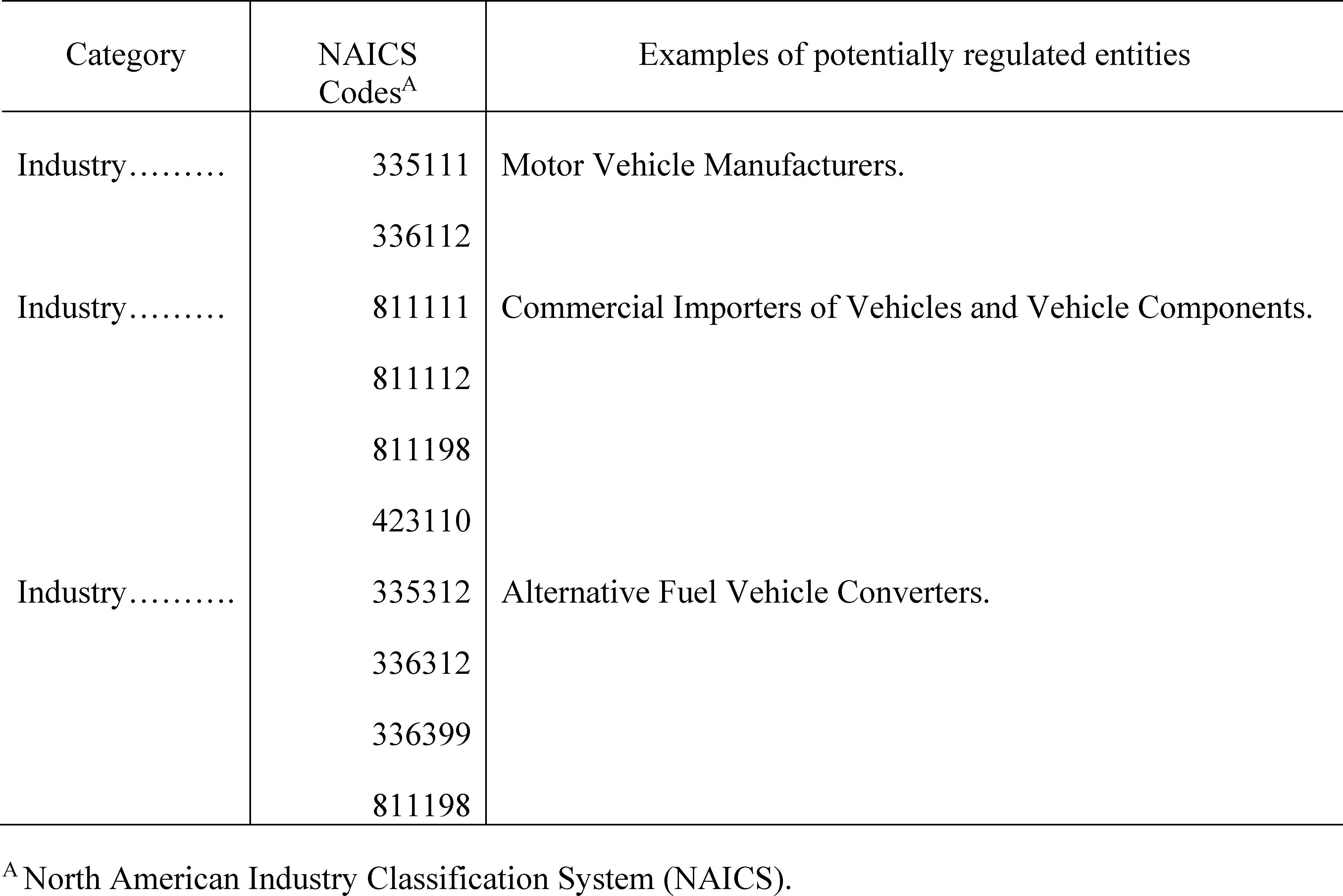
This list is not intended to be exhaustive, but rather provides a guide regarding entities likely to be regulated by this action. To determine whether particular activities may be regulated by this action, you should carefully examine the regulations. You may direct questions regarding the applicability of this action to the person listed in FOR FURTHER INFORMATION CONTACT.
I. Executive Summary
II. Overview of Final Rule
III. Purpose of the Rule
IV. Purpose of Analytical Approach Considered as Part of Decision-Making
V. Regulatory Alternatives Considered
VI. Analytical Approach as Applied to Regulatory Alternatives
VII. What does the analysis show, and what does it mean?
VIII. How do the final standards fulfill the agencies' statutory obligations?
IX. Compliance and Enforcement
X. Regulatory Notices and Analyses
I. Executive Summary
NHTSA (on behalf of the Department of Transportation) and EPA are issuing final rules to adopt and modify standards regulating corporate average fuel economy and tailpipe carbon dioxide (CO2) emissions and use/leakage of other air conditioning refrigerants for passenger cars and light trucks for MYs 2021-2026.[3] These final rules follow the proposal issued in August 2018 and respond to each agency's legal obligation to set standards based on the factors Congress directed them to consider, as well as the direction of the United States Supreme Court in Massachusetts v. EPA, which stated that “there is no reason to think the two agencies cannot both administer their obligations and yet avoid inconsistency.” [4] These standards are the product of significant and ongoing work by both agencies to craft regulatory requirements for the same group of vehicles and vehicle manufacturers. This work aims to facilitate, to the extent possible within the statutory directives issued to each agency, the ability of automobile manufacturers to meet all requirements under both programs with a single national fleet under one national program of fuel economy and tailpipe CO2 emission regulation.
The CAFE and CO2 emissions standards established by these final rules will increase in stringency at 1.5 percent per year from MY 2020 levels over MYs 2021-2026. The “1.5 percent” regulatory alternative is new for the final rule and was not expressly analyzed in the NPRM, but it is a logical outgrowth of the NPRM analysis, being well within the range of alternatives then considered and consistent with discussions by both the agencies and commenters that there are benefits to having standards that increase at the same rate for all fleets. These standards apply to light-duty vehicles, which NHTSA divides for purposes of regulation into passenger cars and light trucks, and EPA divides into passenger cars, light-duty trucks, and medium-duty passenger vehicles (i.e., sport utility vehicles, cross-over utility vehicles, and light trucks). Both the CAFE and CO2 standards are vehicle-footprint-based, as are the standards currently in effect. These standards will become more stringent for each model year from 2021 to 2026, relative to the MY 2020 standards. Generally, the larger the vehicle footprint, the less numerically stringent the corresponding vehicle CO2 and miles-per-gallon (mpg) targets. As a result of the footprint-based standards, the burden of compliance is distributed across all vehicle footprints and across all manufacturers. Each manufacturer is subject to individualized standards for passenger cars and light trucks, in each model year, based on the vehicles it produces. When standards are carefully crafted, both in terms of the footprint curves and the rate of increase in stringency of those curves, manufacturers are not compelled to build vehicles of any particular size or type.
Knowing that many readers are accustomed to considering CAFE and CO2 emissions standards in terms of the mpg and grams-per-mile (g/mi) values that the standards are projected to eventually require, the agencies include those projections here. EPA's standards are projected to require, on an average industry fleet-wide basis, 201 grams per mile (g/mi) of CO2 in model year 2030, while NHTSA's standards are projected to require, on an average industry fleet-wide basis, 40.5 miles per gallon (mpg) in model year 2030. The agencies note that real-world CO2 is typically 25 percent higher and real-world fuel economy is typically 20 percent lower than the CO2 and CAFE compliance values discussed here, and also note that a portion of EPA's expected “CO2” improvements will in fact be made through improvements in minimizing air conditioning leakage and through use of alternative refrigerants, which will not contribute to fuel economy but will contribute toward reductions of climate-related emissions.
In these final rules, NHTSA and EPA are reaching similar conclusions on similar grounds: even though each agency has its own distinct statutory authority and factors, the relevant considerations overlap in many ways. Both agencies recognize that they are balancing the relevant considerations in somewhat different ways from how they may have been balanced previously, as in the 2012 final rule and in EPA's Initial Determination, but the current balancing is called for in light of the facts before the agencies. The balancing in these final rules is also somewhat different from how the agencies balanced their respective considerations in the proposal, in part because of updates to analytical inputs and methodologies, previewed in the NPRM and made in response to public comments, that collectively resulted in changes to the analytical outputs. For example, between the notice and final rule, the agencies updated fuel price projections to somewhat greater values, updated the analysis fleet to MY 2017, updated estimates of the efficacy and cost of fuel-saving technologies, revised procedures for calculating impacts on vehicle sales and scrappage, updated models for estimating highway safety impacts, updated estimates of highway congestion costs, and updated estimates of annual mileage accumulation, holding VMT (before applying the rebound effect) constant between regulatory alternative. Moreover, the cost-benefit analysis conducted for these final rules has even been overtaken by events in many ways over recent weeks. Based upon current events, and for additional reasons discussed in Section VI.D.1 the benefits of saving additional fuel through more stringent standards are potentially even smaller than estimated in this rulemaking analysis.
The standards finalized today fit the pattern of gradual, tough, but feasible stringency increases that take into account real world performance, shifts in fuel prices, and changes in consumer behavior toward crossovers and SUVs and away from more efficient sedans. This approach ensures that manufacturers are provided with sufficient lead time to achieve standards, considering the cost of compliance. The costs to both industry and automotive consumers would have been too high under the standards set forth in 2012, and by lowering the auto industry's costs to comply with the program, with a commensurate reduction in per-vehicle costs to consumers, the standards enhance the ability of the fleet to turn over to newer, cleaner and safer vehicles.
More stringent standards also have the potential for overly aggressive penetration rates for advanced technologies relative to the penetration rates seen in the final standards, especially in the face of an unknown degree of consumer acceptance of both the increased costs and of the technologies themselves—particularly given current projections of relatively low fuel prices during that timeframe. As a kind of insurance policy against future fuel price volatility, standards that increase at 1.5 percent per year for cars and trucks will help to keep fleet fuel economy higher than they would be otherwise when fuel prices are low, which is not improbable over the next several years.[5] At the same time, the standards help to address these issues by maintaining incentives to promote broader deployment of advanced technologies, and so provides a means of encouraging their further penetration while leaving manufacturers alternative technology choices. Steady, gradual increases in stringency ensure that the benefits of reduced GHG emissions and fuel consumption are achieved without the potential for disruption to automakers or consumers.
Standards that increase at 1.5 percent per year represent a reasonable balance of additional technology and required per-vehicle costs, consumer demand for fuel economy, fuel savings and emissions avoided given the foreseeable state of the global oil market and the minimal effect on climate between finalizing 1.5 percent standards versus more stringent standards. The final standards will also result in year-over-year improvements in fleetwide fuel economy, resulting in energy conservation that helps address environmental concerns, including criteria pollutant, air toxic pollutant, and carbon emissions.
The agencies project that under these final standards, required technology costs would be reduced by $86 to $126 billion over the lifetimes of vehicles through MY 2029. Equally important, purchase prices costs to U.S. consumers for new vehicles would be $977 to $1,083 lower, on average, than they would have been if the agencies had retained the standards set forth in the 2012 final rule and originally upheld by EPA in January 2017. While these final standards are estimated to result in 1.9 to 2.0 additional billion barrels of fuel consumed and from 867 to 923 additional million metric tons of CO2 as compared to current estimates of what the standards set forth in 2012 would require, the agencies explain at length below why the overall benefits of the final standards outweigh these additional costs.[6]
For the CAFE program, overall (fleetwide) net benefits vary from $16.1 billion at a 7 percent discount rate to −$13.1 billion at a 3 percent discount rate. For the CO2 program, overall (fleetwide) societal net benefits vary from $6.4 billion at a 7 percent discount rate to −$22.0 billion at a 3 percent discount rate. The net benefits straddle zero, and are very small relative to the scale of reduced required technology costs, which range from $86.3 billion to $126.0 billion for the CAFE and CO2 programs across 7 percent and 3 percent discount rates. Likewise, net benefits are very small relative to the scale of reduced retail fuel savings over the full life of all vehicles manufactured during the 2021 through 2029 model years, which range from $108.6 billion to $185.1 billion for the CAFE and CO2 programs across 7 percent and 3 percent discount rates. Similarly, all of the alternatives have small net benefits, ranging from $18.4 billion to −$31.1 billion for the CAFE and CO2 programs across 7 percent and 3 percent discount rates.[7]
NHTSA and EPA believe their analysis of the final rule represents the best available science, evidence, and methodologies for assessing the impacts of changes in CAFE and CO2 emission standards. In fact, the agencies note that today's analysis represents a marked improvement over prior rulemakings. Previously, the agencies were unable to model the impact of the standards on new vehicle sales or the retirement of older vehicles in the fleet, and, instead, were forced to assume, contrary to economic theory and empirical evidence, that the number of new vehicles sold and older vehicles scrapped remained static across regulatory alternatives. Today's analysis—as commenters to previous rulemakings and EPA's Science Advisory Board have argued is necessary [8] —quantifies the sales and scrappage impacts of the standards, including the associated safety benefits, and represents a significant step forward in agencies' ability to comprehensively analyze the impacts of CAFE and CO2 emission standards.
However, the agencies also believe it is important to be transparent about analytical limitations. For example, EPA's Science Advisory Board stressed that the agencies account for “evolving consumer preferences for performance and other vehicle attributes,” [9] yet due to limitations on the agencies' current ability to model buyers' choices among combinations of various attributes and their costs, the primary analysis does not account for the consumer benefits of other vehicle features that may be sacrificed for costly technologies that improve fuel economy. The agencies' analysis assumes that under these final standards, attributes of new cars and light trucks other than fuel economy would remain identical to those under the baseline standards, so that changes in sales prices and fuel economy would be the only sources of benefits or costs to new car and light truck buyers. In other words, the agencies' primary analysis does not consider that producers will likely respond to buyers' demands by reallocating some their savings in production costs due to lower technology costs to add or improve other attributes that consumers value more highly than the increases in fuel economy the augural standards would have required. The agencies have long debated whether and how best to model the consumer benefits of other vehicle attributes, and note that they have made considerable progress.[10] However, despite these potential analytical shortcomings, the agencies reaffirm that today's analysis represents the most complete and rigorous examination of CAFE and CO2 emission standards to date, and provide decision-makers a powerful analytical tool—especially since the limitations are known, do not bias the central analysis' results, and are afforded due consideration.
In terms of the agencies' respective statutory authorities, EPA is setting national tailpipe CO2 emissions standards for passenger cars and light trucks under section 202(a) of the Clean Air Act (CAA),[11] and taking other actions under its authority to establish metrics and measure passenger car and light truck fleet fuel economy pursuant to the Energy Policy and Conservation Act (EPCA),[12] while NHTSA is setting national corporate average fuel economy (CAFE) standards under EPCA, as amended by the Energy Independence and Security Act (EISA) of 2007.[13] As summarized above and as discussed in much greater detail below, the agencies believe that these represent appropriate levels of CO2 emissions standards and maximum feasible CAFE standards for MYs 2021-2026, pursuant to their respective statutory authorities. Sections III and VIII below contain detailed discussions of both agencies' statutory obligations and authorities.
Section 202(a) of the CAA requires EPA to establish standards for emissions of pollutants from new motor vehicles that cause or contribute to air pollution that may reasonably be anticipated to endanger public health or welfare. Standards under section 202(a) thus take effect only “after providing such period as the Administrator finds necessary to permit the development and application of the requisite technology, giving appropriate consideration to the cost of compliance within such period.” [14] In establishing such standards, EPA must consider issues of technical feasibility, cost, and available lead time, among other things.
EPCA, as amended by EISA, contains a number of provisions governing how NHTSA must set CAFE standards. EPCA requires that the Department of Transportation establish separate passenger car and light truck standards [15] at “the maximum feasible average fuel economy level that the Secretary decides the manufacturers can achieve in that model year,” [16] based on the agency's consideration of four statutory factors: technological feasibility, economic practicability, the effect of other standards of the Government on fuel economy, and the need of the United States to conserve energy.[17] EPCA does not define these terms or specify what weight to give each concern in balancing them—such considerations are left within the discretion of the Secretary of Transportation (delegated to NHTSA) based upon current information. Accordingly, NHTSA interprets these factors and determines the appropriate weighting that leads to the maximum feasible standards given the circumstances present at the time of promulgating each CAFE standard rulemaking. While EISA, for MYs 2011-2020, additionally required that standards increase “ratably” and be set at levels to ensure that the CAFE of the industry-wide combined fleet of new passenger cars and light trucks reach at least 35 mpg by MY 2020,[18] EISA requires that standards for MYs 2021-2030 simply be set at the maximum feasible level as determined by the Secretary (and by delegation, NHTSA).[19]
In the NPRM, the agencies sought comment on a variety of possible changes to existing compliance flexibilities that have been created over the past several years. The vast majority of the existing compliance flexibilities are not being changed, but a small number of flexibilities related to real-world fuel efficiency improvements are being finalized. In addition, EPA will continue to allow manufacturers to make improvements relating to air conditioning refrigerants and leakage and will credit those improvements toward CO2 compliance, and EPA is making no changes in the amounts of credits available. EPA is also not making any changes to the existing CH4 and N2 O standards. EPA is also extending the “0 g/mi upstream” incentive for electric vehicles beyond its current sunset of MY 2021, through MY 2026. EPA is also establishing a credit multiplier for natural gas vehicles through the 2026 model year. Otherwise, compliance flexibilities in the two programs do not change significantly for the final rule. These changes should help to streamline manufacturer use of those flexibilities in certain respects. While manufacturers and suppliers sought a number of other additional compliance flexibilities, the agencies have concluded that the aforementioned existing flexibilities are reasonable and appropriate, and that additional flexibilities are not justified.
Table I-1 and Table I-2 present the total costs, benefits, and net benefits for the 2021-2026 preferred alternative CAFE and CO2 levels, relative to the MY 2022-2025 existing/augural standards (with the MY 2025 standards repeated for MY 2026) and current MY 2021 standard. The preferred alternative exhibits a stringency rate increase of 1.5 percent per year for both passenger cars and light trucks. The values in Table I-1 and Table I-2 display (in total and annualized forms) costs for all MYs 1978-2029 vehicles, and the benefits and net benefits represent the impacts of the standards over the full lifetimes of the vehicles sold or projected to be sold during model years 1978-2029.
For this analysis, negative signs are used for changes in costs or benefits that decrease from those that would have resulted from the existing/augural standards. Any changes that would increase either costs or benefits are shown as positive changes. Thus, an alternative that decreases both costs and benefits, will show declines (i.e., a negative sign) in both categories. From Table I-1 and Table I-2, the preferred alternative (Alternative 3) is estimated to decrease costs relative to the baseline by $182 to $280 billion over the lifetime of MYs 1978-2029 passenger vehicles (range determined by discount rate across both CAFE and CO2 programs). It will also decrease benefits from $175 to $294 billion over the life of these MY fleets. The net impact will be a decrease from $22 billion to an increase of $16 billion in total net benefits to society over this roughly 52-year timeframe. Annualized, this amounts to roughly −$0.8 to 1.2 billion in net benefits per year.


Table I-3 and Table I-4 lists costs, benefits, and net benefits for all seven alternatives that were examined.


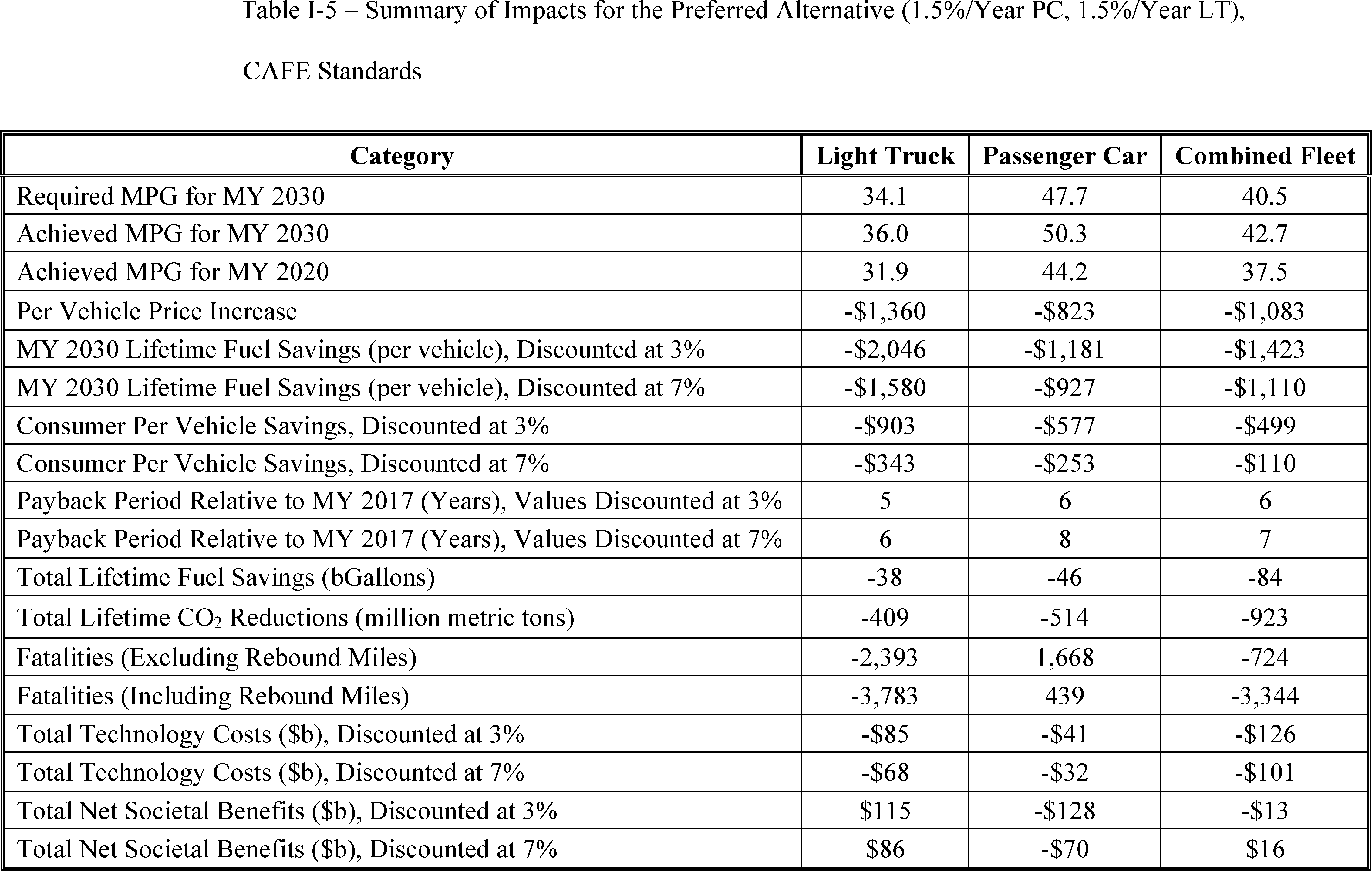
Table I-5 and Table I-6 show a summary of various impacts of the preferred alternative for CAFE and CO2 standards. Impacts are presented in monetized and non-monetized values, as well as from the perspective of society and the consumer.

The agencies note that the NPRM drew more public comments (and, particularly, more pages of substantive comments) than any rulemaking in the history of the CAFE or CO2 tailpipe emissions programs—exceeding 750,000 comments. The agencies recognized in the NPRM that the proposal was significantly different from the final rules set forth in 2012, and explained at length the reasons for those differences—namely, that new information and considerations, along with an expanded and updated analysis, had led to different tentative conclusions. Today's final rules represent a further evolution of the work that supported the proposal, based on improved quantitative methodology and in careful consideration of the hundreds of thousands of public comments and deep reflection on the serious issues before the agencies. Simply put, the agencies have heard the comments, and today's analysis and decision reflect the agencies' grappling with the issues commenters raised, as well as all of the other information before the agencies. These programs and issues are weighty, and the agencies believe that a reasonable balance has been struck in these final rules between the many competing national needs that these regulatory programs collectively address.
II. Overview of Final Rule
A. Summary of Proposal
In the NPRM, the National Highway Traffic Safety Administration (NHTSA) and the Environmental Protection Agency (EPA) (collectively, “the agencies”) proposed the “Safer Affordable Fuel-Efficient (SAFE) Vehicles Rule for Model Years 2021-2026 Passenger Cars and Light Trucks” (SAFE Vehicles Rule). The proposed SAFE Vehicles Rule would set Corporate Average Fuel Economy (CAFE) and carbon dioxide (CO2) emissions standards, respectively, for passenger cars and light trucks manufactured for sale in the United States in model years (MYs) 2021 through 2026.[20]
The agencies explained that they must act to propose and finalize these standards and do not have discretion to decline to regulate. Congress requires NHTSA to set CAFE standards for each model year.[21] Congress also requires EPA to set emissions standards for light-duty vehicles if EPA has made an “endangerment finding” that the pollutant in question—in this case, CO2—“cause[s] or contribute[s] to air pollution which may reasonably be anticipated to endanger public health or welfare.” [22] NHTSA and EPA proposed the standards concurrently because tailpipe CO2 emissions standards are directly and inherently related to fuel economy standards,[23] and, if finalized, the rules would apply concurrently to the same fleet of vehicles. By working together to develop the proposals, the agencies aimed to reduce regulatory burden on industry and improve administrative efficiency.
The agencies discussed some of the history leading to the proposal, including the 2012 final rule, the expectations regarding a mid-term evaluation as required by EPA regulation, and the rapid process over 2016 and early 2017 by which EPA issued its first Final Determination that the CO2 standards set in 2012 for MYs 2022-2025 remained appropriate based on the information then before the EPA Administrator.[24] The agencies also discussed President Trump's direction in March 2017 to restore the original mid-term evaluation timeline, and EPA's subsequent information-gathering process and announcement that it would reconsider the January 2017 Determination.[25] EPA ultimately concluded that the standards set in 2012 for MYs 2022-2025 were no longer appropriate.[26] For NHTSA, in turn, the “augural” CAFE standards for MYs 2022-2025 were never final, and as explained in the 2012 final rule, NHTSA was obligated from the beginning to undertake a new rulemaking to set CAFE standards for MYs 2022-2025.
The NPRM thus began the rulemaking process for both agencies to establish new standards for MYs 2022-2025 passenger cars and light trucks. Standards were concurrently proposed for MY 2026 in order to provide regulatory stability for as many years as is legally permissible for both agencies together. The NPRM also included revised standards for MY 2021 passenger cars and light trucks, because the agencies tentatively concluded, based on the information and analysis then before them, that the CAFE standards previously set for MY 2021 were no longer maximum feasible, and the CO2 standards previously set for MY 2021 were no longer appropriate. Agencies always have authority under the Administrative Procedure Act to revisit previous decisions in light of new facts, as long as they provide notice and an opportunity for comment, and the agencies stated that it is plainly the best practice to do so when changed circumstances so warrant.[27]
The NPRM proposed to maintain the CAFE and CO2 standards applicable in MY 2020 for MYs 2021-2026, and took comment on a wide range of alternatives, including different stringencies and retaining existing CO2 standards and the augural CAFE standards.[28] Table II-1, Table II-2, and Table II-3 show the estimates, under the NPRM analysis, of what the MY 2020 CAFE and CO2 curves would translate to, in terms of miles per gallon (mpg) and grams per mile (g/mi), in MYs 2021-2026, as well as the regulatory alternatives considered in the NPRM. In addition to retaining the MY 2020 CO2 standards through MY 2026, EPA proposed and sought comment on excluding air conditioning refrigerants and leakage, and nitrous oxide and methane emissions for compliance with CO2 standards after model year 2020, in order to improve harmonization with the CAFE program. EPA also sought comment on whether to change existing methane and nitrous oxide standards that were finalized in the 2012 rule. The proposal was accompanied by a 1,600 page Preliminary Regulatory Impact Analysis (PRIA) and, for NHTSA, a 500 page Draft Environmental Impact Statement (DEIS), with more than 800 pages of appendices and the entire CAFE model, including the software source code and documentation, all of which were also subject to comment in their entirety and all of which received significant comments.


The agencies explained in the NPRM that new information had been gathered and new analysis performed since publication of the 2012 final rule establishing CAFE and CO2 standards for MYs 2017 and beyond and since issuance of the 2016 Draft TAR and EPA's 2016 and early 2017 “mid-term evaluation” process. This new information and analysis helped lead the agencies to the tentative conclusion that holding standards constant at MY 2020 levels through MY 2026 was maximum feasible, for CAFE purposes, and appropriate, for CO2 purposes.
The agencies further explained that technologies had played out differently in the fleet from what the agencies previously assumed: That while there remain a wide variety of technologies available to improve fuel economy and reduce CO2 emissions, it had become clear that there were reasons to temper previous optimism about the costs, effectiveness, and consumer acceptance of a number of technologies. In addition, over the years between the previous analyses and the NPRM, automakers had added considerable amounts of technologies to their new vehicle fleets, meaning that the agencies were no longer free to make certain assumptions about how some of those technologies could be used going forward. For example, some technologies that could be used to improve fuel economy and reduce emissions had not been used entirely for that purpose, and some of the benefit of these technologies had gone instead toward improving other vehicle attributes. Other technologies had been tried, and had been met with significant customer acceptance issues. The agencies underscored the importance of reflecting the fleet as it stands today, with the technology it has and as that technology has been used, and considering what technology remains on the table at this point, whether and when it can realistically be available for widespread use in production, and how much it would cost to implement.
The agencies also acknowledged the math of diminishing returns: As CAFE and CO2 emissions standards increase in stringency, the benefit of continuing to increase in stringency decreases. In mpg terms, a vehicle owner who drives a light vehicle 15,000 miles per year (a typical assumption for analytical purposes) [31] and trades in a vehicle with fuel economy of 15 mpg for one with fuel economy of 20 mpg, will reduce their annual fuel consumption from 1,000 gallons to 750 gallons—saving 250 gallons annually. If, however, that owner were to trade in a vehicle with fuel economy of 30 mpg for one with fuel economy of 40 mpg, the owner's annual gasoline consumption would drop from 500 gallons/year to 375 gallons/year—only 125 gallons even though the mpg improvement is twice as large. Going from 40 to 50 mpg would save only 75 gallons/year. Yet each additional fuel economy improvement becomes much more expensive as the easiest to achieve low-cost technological improvement options are chosen. In CO2 terms, if a vehicle emits 300 g/mi CO2, a 20 percent improvement is 60 g/mi, so the vehicle would emit 240 g/mi; but if the vehicle emits 180 g/mi, a 20 percent improvement is only 36 g/mi, so the vehicle would get 144 g/mi. In order to continue achieving similarly large (on an absolute basis) emissions reductions, the percentage reduction must also continue to increase.
Related, average real-world fuel economy is lower than average fuel economy required under CAFE and CO2 standards. The 2012 Federal Register notice announcing augural CAFE and CO2 standards extending through MY 2025 indicated that, if met entirely through the application of fuel-saving technology, the MY 2025 CO2 standards would result in an average requirement equivalent to 54.5 mpg. However, because the CO2 standards provide credit for reducing leakage of AC refrigerants and/or switching to lower-GWP refrigerants, and these actions do not affect fuel economy, the notice explained that the corresponding fuel economy requirement (under the CAFE program) would be 49.7 mpg. These estimates were based on a market forecast grounded in the MY 2008 fleet. The notice also presented analysis using a market forecast grounded in the MY 2010 fleet, showing a 48.7 mpg average CAFE requirement.
In the real world, fuel economy is, on average, about 20% lower than as measured under regulatory test procedures. In the real world, then, these new standards were estimated to require 39.0-39.8 mpg.
Today's analysis indicates that the requirements under the baseline/augural CAFE standards would average 46.6 mpg in MY 2029. The lower value results from changes in the fleet forecast which reflects consumer preference for larger vehicles than was forecast for the 2012 rulemaking. In the real world, the requirements average about 37.1 mpg. Under the final standards issued today, the regulatory test procedure requirements average 40.5 mpg, corresponding to 33.2 mpg in the real world. Buyers of new vehicles experience real-world fuel economy, with levels varying among drivers (due to a wide range of factors). Vehicle fuel economy labels provide average real-world fuel economy information to buyers.

Vehicle owners also face fuel prices at the pump. The agencies noted in the NPRM that when fuel prices are high, the value of fuel saved may be enough to offset the cost of further fuel economy/emissions reduction improvements, but the agencies recognized that then-current projections of fuel prices by the Energy Information Administration did not indicate particularly high fuel prices in the foreseeable future. The agencies explained that fundamental structural shifts had occurred in global oil markets since the 2012 final rule, largely due to the rise of U.S. production and export of shale oil. The consequence over time of diminishing returns from more stringent fuel economy/emissions reduction standards, especially when combined with relatively low fuel prices, is greater difficulty for automakers to find a market of consumers willing to buy vehicles that meet the increasingly stringent standards. American consumers have long demonstrated that in times of relatively low fuel prices, fuel economy is not a top priority for the majority of them, even when highly fuel efficient vehicle models are available.
The NPRM analysis sought to improve how the agencies captured the effects of higher new vehicle prices on fleet composition as a whole by including an improved model for vehicle scrappage rates. As new vehicle prices increase, consumers tend to continue using older vehicles for longer, slowing fleet turnover and thus slowing improvements in fleet-wide fuel economy, reductions in CO2 emissions, reductions in criteria pollutant emissions, and advances in safety. That aspect of the analysis was also driven by the agencies' updated estimates of average per-vehicle cost increases due to higher standards, which were several hundred dollars higher than previously estimated. The agencies cited growing concerns about affordability and negative equity for many consumers under these circumstances, as loan amounts grow and loan terms extend.
For all of the above reasons, the agencies proposed to maintain the MY 2020 fuel economy and CO2 emissions standards for MYs 2021-2026. The agencies explained that they estimated, relative to the standards for MYs 2021-2026 put forth in 2012, that an additional 0.5 million barrels of oil would be consumed per day (about 2 to 3 percent of projected U.S. consumption) if that proposal were finalized, but that they also expected the additional fuel costs to be outweighed by the cost savings from new vehicle purchases; that more than 12,700 on-road fatalities and significantly more injuries would be prevented over the lifetimes of vehicles through MY 2029 as compared to the standards set forth in the 2012 final rule over the lifetimes of vehicles as more new and safer vehicles are purchased than the current (and augural) standards; and that environmental impacts, on net, would be relatively minor, with criteria and toxic air pollutants not changing noticeably, and with estimated atmospheric CO2 concentrations increasing by 0.65 ppm (a 0.08 percent increase), which the agencies estimated would translate to 0.003 degrees Celsius of additional temperature increase relative to the standards finalized in 2012.
Under the NPRM analysis, the agencies tentatively concluded that maintaining the MY 2020 curves for MYs 2021-2026 would save American auto consumers, the auto industry, and the public a considerable amount of money as compared to EPA retaining the previously-set CO2 standards and NHTSA finalizing the augural standards. The agencies explained that this had been identified as the preferred alternative, in part, because it appeared to maximize net benefits compared to the other alternatives analyzed, and recognizing the statutory considerations for both agencies. Relative to the standards issued in 2012, under CAFE standards, the NPRM analysis estimated that costs would decrease by $502 billion overall at a three-percent discount rate ($335 billion at a seven-percent discount rate) and benefits were estimated to decrease by $326 billion at a three-percent discount rate ($204 billion at a seven-percent discount rate). Thus, net benefits were estimated to increase by $176 billion at a three-percent discount rate and $132 billion at a seven-percent discount rate. The estimated impacts under CO2 standards were estimated to be similar, with net benefits estimated to increase by $201 billion at a three-percent discount rate and $141 billion at a seven-percent discount rate.
The NPRM also sought comment on a variety of potential changes to NHTSA's and EPA's compliance programs for CAFE and CO2 as well as related programs, including questions about automaker requests for additional flexibilities and agency interest in reducing market-distorting incentives and improving transparency; and on a proposal to withdraw California's CAA preemption waiver for its “Advanced Clean Car” regulations, with an accompanying discussion of preemption of State standards under EPCA.[32] The agencies sought comment broadly on all aspects of the proposal.
B. Public Participation Opportunities and Summary of Comments
The NPRM was published on NHTSA's and EPA's websites on August 2, 2018, and published in the Federal Register on August 24, 2018, beginning a 60-day comment period. The agencies subsequently extended the official comment period for an additional three days, and left the dockets open for more than a year after the start of the comment period, considering late comments to the extent practicable. A separate Federal Register notice also published on August 24, 2018, which announced the locations, dates, and times of three public hearings to be held on the proposal: One in Fresno, California, on September 24, 2018; one in Dearborn, Michigan, on September 25, 2018; and one in Pittsburgh, Pennsylvania, on September 26, 2018. Each hearing started at 10 a.m. local time; the Fresno hearing ended at 5:10 p.m. and resulted in a 235 page transcript; the Dearborn hearing ran until 5:26 p.m. and resulted in a 330 page transcript; and the Pittsburgh hearing ran until 5:06 p.m. and also resulted in a 330 page transcript. Each hearing also collected several hundred pages of comments from participants, in addition to the hearing transcripts.
Besides the comments submitted as part of the public hearings, NHTSA's docket received a total of 173,359 public comments in response to the proposal as of September 18, 2019, and EPA's docket a total of 618,647 public comments, for an overall total of 792,006. NHTSA also received several hundred comments on its DEIS to the separate DEIS docket. While the majority of individual comments were form letters, the agencies received over 6,000 pages of substantive comments on the proposal.
Many commenters generally supported the proposal and many commenters opposed it. Commenters supporting the proposal tended to cite concerns about the cost of new vehicles, while commenters opposing the proposal tended to cite concerns about additional fuel expenditures and the impact on climate change. Many comments addressed the modeling used for the analysis, and specifically the inclusion, operation, and results of the sales and scrappage modules that were part of the NPRM's analysis, while many addressed the NPRM's safety findings and the role that those findings played in the proposal's justification. Many other comments addressed California's standards and role in Federal decision-making; as discussed above, those comments are further summarized and responded to in the separate Federal Register notice published in September 2019. Nearly every aspect of the NPRM's analysis and discussion received some level of comment by at least one commenter. The comments received, as a whole, were both broad and deep, and the agencies appreciate the level of engagement of commenters in the public comment process and the information and opinions provided.
C. Changes in Light of Public Comments and New Information
The agencies made a number of changes to the analysis between the NPRM and the final rule in response to public comments and new information that was received in those comments or otherwise became available to the agencies. While these changes, their rationales, and their effects are discussed in detail in the sections below, the following represents a high-level list of some of the most significant changes:
- Some regulatory alternatives were dropped from consideration, and one was added;
- updated analysis fleet, and changes to technologies on “baseline” vehicles within the fleet to reflect better their current properties and improve modeling precision;
- no civil penalties assumed to be paid after MY 2020 under CAFE program;
- updates and expansions in accounting for certain over-compliance credits, including early credits earned in EPA's program;
- updates and expansions to CAFE Model's technology paths;
- updates to inputs defining the range of manufacturer-, technology-, and product-specific constraints;
- updates to allow the model to adopt a more advanced technology if it is more cost-effective than an earlier technology on the path;
- precision improvements to the modeling of A/C efficiency and off-cycle credits;
- updates to model's “effective cost” metric;
- extended explicit simulation of technology application through MY 2050;
- expanded presentation of the results to include “calendar year” analysis;
- quantifying different types of health impacts from changes in air pollution, rather than only accounting for such impacts in aggregate estimates of the social costs of air pollution;
- updated costs to 2018 dollars;
- updated fuel costs based on the AEO 2019 version of NEMS;
- a variety of technology updates in response to comments and new information;
- updated accounting of rebound VMT between regulatory alternatives;
- updated estimates of the macroeconomic cost of petroleum dependence;
- updated response of total new vehicle sales to increases in fuel efficiency and price; and
- updated response of vehicle retirement rates to changes in new vehicle fuel efficiency and transaction price.
Sections IV and VI below discuss these updates in significant detail.
D. Final Standards—Stringency
As explained above, the agencies have chosen to set CAFE and CO2 standards that increase in stringency by 1.5 percent year over year for MYs 2021-2026. Separately, EPA has decided to retain the A/C refrigerant and leakage and CH4 and N2 O standards set forth in 2012 for MYs 2021 and beyond, and the stringency of the CO2 standards in this final rule reflect the “offset” also established in 2012 based on assumptions made at that time about anticipated HFC emissions reductions.
When the agencies state that stringency will increase at 1.5 percent per year, that means that the footprint curves which actually define the standards for CAFE and CO2 emissions will become more stringent at 1.5 percent per year. Consistent with Congress's direction in EISA to set CAFE standards based on a mathematical formula, which EPA harmonized with for the CO2 emissions standards, the standard curves are equations, which are slightly different for CAFE and CO2, and within each program, slightly different for passenger cars and light trucks. Each program has a basic equation for a fleet standard, and then values that change to cause the stringency changes are the coefficients within the equations. For passenger cars, consistent with prior rulemakings, NHTSA is defining fuel economy targets as follows:

where:
TARGETFE is the fuel economy target (in mpg) applicable to a specific vehicle model type with a unique footprint combination,
a is a minimum fuel economy target (in mpg),
b is a maximum fuel economy target (in mpg),
c is the slope (in gallons per mile per square foot, or gpm, per square foot) of a line relating fuel consumption (the inverse of fuel economy) to footprint, and
d is an intercept (in gpm) of the same line.
Here, MIN and MAX are functions that take the minimum and maximum values, respectively, of the set of included values. For example, MIN[40,35] = 35 and MAX (40, 25) = 40, such that MIN[MAX (40, 25), 35] = 35.
For light trucks, also consistent with prior rulemakings, NHTSA is defining fuel economy targets as follows:

where:
TARGETFE is the fuel economy target (in mpg) applicable to a specific vehicle model type with a unique footprint combination,
a, b, c, and d are as for passenger cars, but taking values specific to light trucks,
e is a second minimum fuel economy target (in mpg),
f is a second maximum fuel economy target (in mpg),
g is the slope (in gpm per square foot) of a second line relating fuel consumption (the inverse of fuel economy) to footprint, and
h is an intercept (in gpm) of the same second line.
The final CAFE standards (described in terms of their footprint-based curves) are as follows, with the values for the coefficients changing over time:

These equations are presented graphically below, where the x-axis represents vehicle footprint and the y-axis represents fuel economy, showing that in the CAFE context, targets are higher (fuel economy) for smaller footprint vehicles and lower for larger footprint vehicles:


EPCA, as amended by EISA, requires that any manufacturer's domestically-manufactured passenger car fleet must meet the greater of either 27.5 mpg on average, or 92 percent of the average fuel economy projected by the Secretary for the combined domestic and non-domestic passenger automobile fleets manufactured for sale in the U.S. by all manufacturers in the model year, which projection shall be published in the Federal Register when the standard for that model year is promulgated in accordance with 49 U.S.C. 32902(b).[33] Any time NHTSA establishes or changes a passenger car standard for a model year, the MDPCS for that model year must also be evaluated or re-evaluated and established accordingly. Thus, this final rule establishes the applicable MDPCS for MYs 2021-2026. Table II-8 lists the minimum domestic passenger car standards.

EPA CO2 standards are as follows. Rather than expressing these standards as linear functions with accompanying minima and maxima, similar to the approach NHTSA has followed since 2005 in specifying attribute-based standards, the following tables specify flat standards that apply below and above specified footprints, and a linear function that applies between those footprints. The two approaches are mathematically identical. For passenger cars with a footprint of less than or equal to 41 square feet, the gram/mile CO2 target value is selected for the appropriate model year from Table II-9:

For passenger cars with a footprint of greater than 56 square feet, the gram/mile CO2 target value is selected for the appropriate model year from Table II-10:

For passenger cars with a footprint that is greater than 41 square feet and less than or equal to 56 square feet, the gram/mile CO2 target value is calculated using the following equation and rounded to the nearest 0.1 grams/mile.
Target CO2 = [a × f] + b
Where f is the vehicle footprint and a and b are selected from Table II-11 for the appropriate model year:

For light trucks with a footprint of less than or equal to 41 square feet, the gram/mile CO2 target value is selected for the appropriate model year from Table II-12:

For light trucks with a footprint greater than the minimum value specified in the table below for each model year, the gram/mile CO2 target value is selected for the appropriate model year from Table II-13:

For light trucks with a footprint that is greater than 41 square feet and less than or equal to the maximum footprint value specified in Table II-14 below for each model year, the gram/mile CO2 target value is calculated using the following equation and rounded to the nearest 0.1 grams/mile.
Target CO2 = (a × f) + b
Where f is the footprint and a and b are selected from Table II-14 below for the appropriate model year:

These equations are presented graphically below, where the x-axis represents vehicle footprint and the y-axis represents the CO2 target. The targets are lower for smaller footprint vehicles and higher for larger footprint vehicles:


Except that EPA elected to apply a slightly different slope when defining passenger car targets, CO2 targets may be expressed as direct conversion of fuel economy targets, as follows:

where 8887 g/gal relates grams of CO2 emitted to gallons of fuel consumed, and OFFSET reflects the fact that that HFC emissions from lower-GWP A/C refrigerants and less leak-prone A/C systems are counted toward average CO2 emissions, but EPCA provides no basis to count reduced HFC emissions toward CAFE levels.
For the reader's benefit, Table II-15, Table II-16, and Table II-17 show the estimates, under the final rule analysis, of what the MYs 2021-2026 CAFE and CO2 curves would translate to, in terms of miles per gallon (mpg) and grams per mile (g/mi).

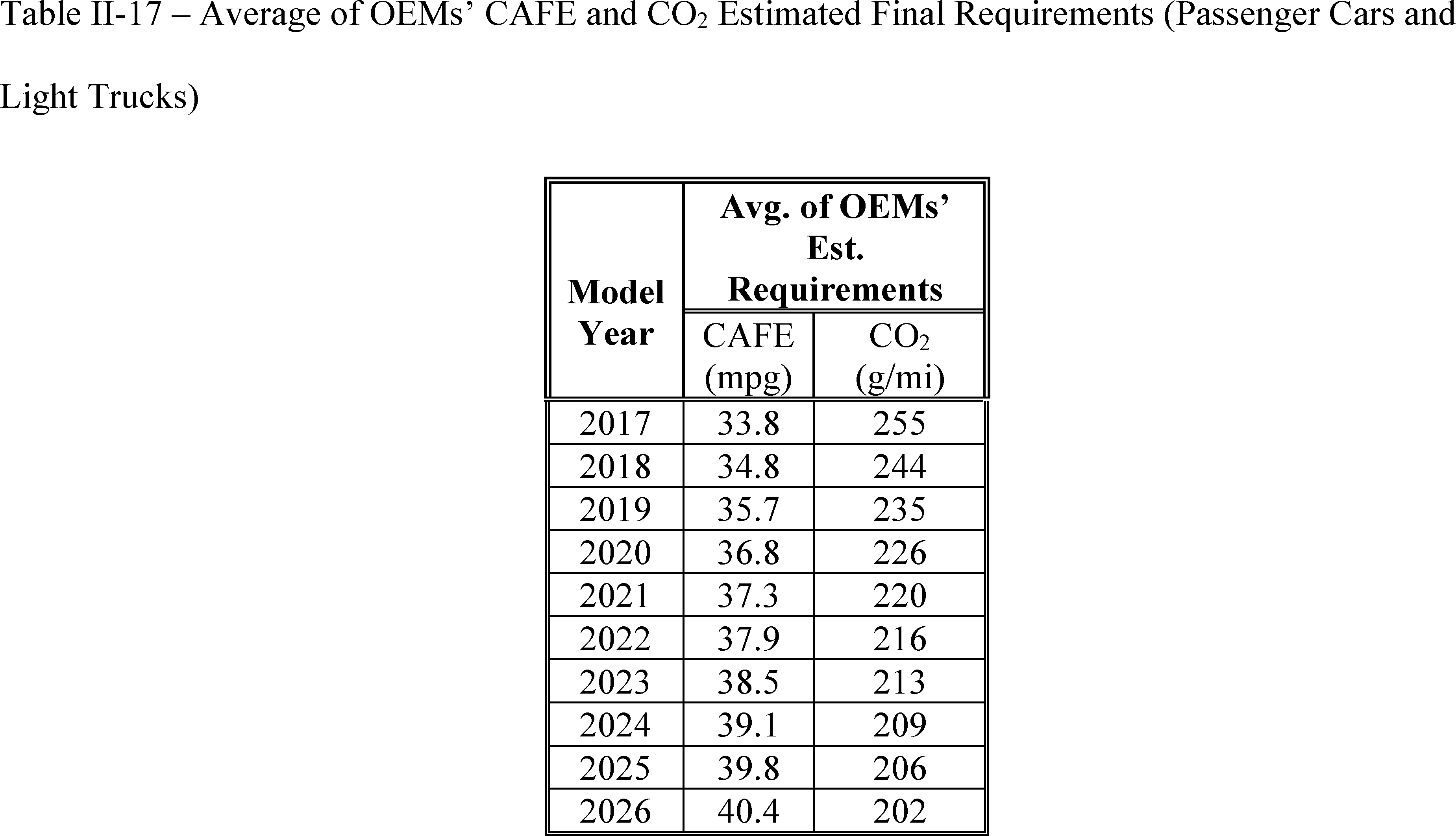
As the following tables demonstrate, averages of manufacturers' estimated requirements are more stringent (i.e., for CAFE, higher, and for CO2, lower) under the final standards than under the proposed standards:


E. Final Standards—Impacts
This section summarizes the estimated costs and benefits of the MYs 2021-2026 CAFE and CO2 emissions standards for passenger cars and light trucks, as compared to the regulatory alternatives considered. These estimates helped inform the agencies' choices among the regulatory alternatives considered and provide further confirmation that the final standards are maximum feasible, for NHTSA, and appropriate, for EPA. The costs and benefits estimated to result from the CAFE standards are presented first, followed by those estimated to result from the CO2 standards. For several reasons, the estimates for costs and benefits presented for the different programs, while consistent, are not identical. NHTSA's and EPA's standards are projected to result in slightly different fuel efficiency improvements. EPA's CO2 standard is nominally more stringent in part due to its assumptions about manufacturers' use of air conditioning leakage/refrigerant replacement credits, which are expected to result in reduced emissions of HFCs. NHTSA's final standards are based solely on assumptions about fuel economy improvements, and do not account for emissions reductions that do not relate to fuel economy. In addition, the CAFE and CO2 programs offer somewhat different program flexibilities and provisions, primarily because NHTSA is statutorily prohibited from considering some flexibilities when establishing CAFE standards, while EPA is not.[34] The analysis underlying this final rule reflects many of those additional EPA flexibilities, which contributes to differences in how the agencies estimate manufacturers could comply with the respective sets of standards, which in turn contributes to differences in estimated impacts of the standards. These differences in compliance flexibilities are discussed in more detail in Section IX below.
Table II-20 to Table II-23 present all subcategories of costs and benefits of this final rule for all seven alternatives proposed. Costs include application of fuel economy technology to new vehicles, consumer surplus, crash costs due to changes in VMT, as well as, noise and congestion. Benefits include fuel savings, consumer surplus, refueling time, and clean air.


F. Other Programmatic Elements
1. Compliance and Flexibilities
Automakers seeking to comply with the CAFE and CO2 standards are generally expected to add fuel economy-improving technologies to their new vehicles to boost their overall fleet fuel economy levels. Readers will remember that improving fuel economy directly reduces CO2 emissions, because CO2 is a natural and inevitable byproduct of fossil fuel combustion to power vehicles. The CAFE and CO2 programs contain a variety of compliance provisions and flexibilities to accommodate better automakers' production cycles, to reward real-world fuel economy improvements that cannot be reflected in the 1975-developed test procedures, and to incentivize the production of certain types of vehicles. While the agencies sought comment on a broad variety of changes and potential expansions of the programs' compliance flexibilities in the NPRM, the agencies determined, after considering the comments, to make a few changes to the flexibilities proposed in the NPRM in this final rule. The most noteworthy change is the retention, in the CO2 program, of the flexibilities that allow automakers to continue to use HFC reductions toward their CO2 compliance, and that extend the “0 grams/mile” assumption for electric vehicles through MY 2026 (i.e., recognizing only the tailpipe emissions of full battery-electric vehicles and not recognizing the upstream emissions caused by the electricity usage of those vehicles). In the NPRM, EPA had proposed to remove and sought comment on removing those flexibilities from the CO2 program, but determined not to remove them in this final rule. EPA and NHTSA are also removing from the programs, starting in MY 2022, the credit/FCIV for full-size pickup trucks that are either hybrids or over-performing by a certain amount relative to their targets, and allowing technology suppliers to begin the petition process for off-cycle credits/adjustments.
Table II-24, Table II-25, Table II-26, and Table II-27 provide a summary of the various compliance provisions in the two programs; their authorities; and any changes included as part of this final rule:


Providing a technology neutral basis by which manufacturers meet fuel economy and CO2 emissions standards encourages an efficient and level playing field. The agencies continue to have a desire to minimize incentives that disproportionately favor one technology over another. Some of this may involve regulations established by other Federal agencies. In the near future, NHTSA and EPA intend to work with other relevant Federal agencies to pursue regulatory means by which we can further ensure technology neutrality in this field.
2. Preemption/Waiver
As discussed above, the issues of Clean Air Act waivers of preemption under Section 209 and EPCA/EISA preemption under 49 U.S.C. 32919 are not addressed in today's final rule, as they were the subject of a separate final rulemaking action by the agencies in September 2019. While many comments were received in response to the NPRM discussion of those issues, those comments have been addressed and responded to as part of that separate rulemaking action.
III. Purpose of the Rule
The Administrative Procedure Act (APA) requires agencies to incorporate in their final rules a “concise general statement of their basis and purpose.” [36] While the entire preamble document represents the agencies' overall explanation of the basis and purpose for this regulatory action, this section within the preamble is intended as a direct response to that APA (and related CAA) requirements. Executive Order 12866 further states that “Federal agencies should promulgate only such regulations as are required by law, are necessary to interpret the law, or are made necessary by compelling public need, such as material failures of private markets to protect or improve the health and safety of the public, the environment, or the well-being of the American people.” [37] Section III.C of the FRIA accompanying this rulemaking discusses at greater length the question of whether a market failure exists that these final rules may address.
NHTSA and EPA are legally obligated to set CAFE and GHG standards, respectively, and do not have the authority to decline to regulate.[38] The agencies are issuing these final rules to fulfill their respective statutory obligations to provide maximum feasible fuel economy standards and limit emissions of pollutants from new motor vehicles which have been found to endanger public health and welfare (in this case, specifically carbon dioxide (CO2); EPA has already set standards for methane (CH4), nitrous oxide (N2 O), and hydrofluorocarbons (HFCs) and is not revising them in this rule). Continued progress in meeting these statutory obligations is both legally necessary and good for America—greater energy security and reduced emissions protect the American public. The final standards continue that progress, albeit at a slower rate than the standards finalized in 2012.
National annual gasoline consumption and CO2 emissions currently total about 140 billion gallons and 5,300 million metric tons, respectively. The majority of this gasoline (about 130 billion gallons) is used to fuel passenger cars and light trucks, such as will be covered by the CAFE and CO2 standards issued today. Accounting for both tailpipe emissions and emissions from “upstream” processes (e.g., domestic refining) involved in producing and delivering fuel, passenger cars and light trucks account for about 1,500 million metric tons (mmt) of current annual CO2 emissions. The agencies estimate that under the standards issued in 2012, passenger car and light truck annual gasoline consumption would steadily decline, reaching about 80 billion gallons by 2050. The agencies further estimate that, because of this decrease in gasoline consumption under the standards issued in 2012, passenger car and light truck annual CO2 emissions would also steadily decline, reaching about 1,000 mmt by 2050. Under the standards issued today, the agencies estimate that, instead of declining from about 140 billion gallons annually today to about 80 billion gallons annually in 2050, passenger car and light truck gasoline consumption would decline to about 95 billion gallons. The agencies correspondingly estimate that instead of declining from about 1,500 mmt annually today to about 1,000 mmt annually in 2050, passenger car and light truck CO2 emissions would decline to about 1,100 mmt. In short, the agencies estimate that under the standards issued today, annual passenger car and light truck gasoline consumption and CO2 emissions will continue to steadily decline over the next three decades, even if not quite as rapidly as under the previously-issued standards.
The agencies also estimate that these impacts on passenger car and light truck gasoline consumption and CO2 emissions will be accompanied by a range of other energy- and climate-related impacts, such as reduced electricity consumption (because today's standards reduce the estimated rate at which the market might shift toward electric vehicles) and increased CH4 and N2 O emissions. These estimated impacts, discussed below and in the FEIS accompanying today's notice, are dwarfed by estimated impacts on gasoline consumption and CO2 emissions.
As explained above, these final rules set or amend fuel economy and carbon dioxide standards for model years 2021-2026. Many commenters argued that it was not appropriate to amend previously-established CO2 and CAFE standards, generally because those commenters believed that the administrative record established for the 2012 final rule and EPA's January 2017 Final Determination was superior to the record that informed the NPRM, and that that prior record led necessarily to the policy conclusion that the previously-established standards should remain in place.[39] Some commenters similarly argued that EPA's Revised Final Determination—which, for EPA, preceded this regulatory action—was invalid because, they allege, it did not follow the procedures established for the mid-term evaluation that EPA codified into regulation,[40] and also because the Revised Final Determination was not based on the prior record.[41]
The agencies considered a range of alternatives in the proposal, including the baseline/no action alternative of retaining the existing EPA carbon dioxide standards. As the agencies explained in the proposal, the proposal was entirely de novo, based on an entirely new analysis reflecting the best and most up-to-date information available to the agencies.[42] This rulemaking action is separate and distinct from EPA's Revised Final Determination, which itself was neither a proposed nor a final decision that the standards “must” be revised. EPA retained full discretion in this rulemaking to revise the standards or not revise them. In any event, the case law is clear that agencies are free to reconsider their prior decisions.[43] With that legal principle in mind, the agencies agree with commenters that the amended (and new) CO2 and CAFE standards must be consistent with the CAA and EPCA/EISA, respectively, and this preamble and the accompanying FRIA explain in detail why the agencies believe they are consistent. The section below discusses briefly the authority given to the agencies by their respective governing statutes, and the factors that Congress directed the agencies to consider as they exercise that authority in pursuit of fulfilling their statutory obligations.
A. EPA's Statutory Requirements
EPA is setting national CO2 standards for passenger cars and light trucks under Section 202(a) of the Clean Air Act (CAA).[44] Section 202(a) of the CAA requires EPA to establish standards for emissions of pollutants from new motor vehicles which cause or contribute to air pollution which may reasonably be anticipated to endanger public health or welfare.[45] In establishing such standards, EPA considers issues of technical feasibility, cost, available lead time, and other factors. Standards under section 202(a) thus take effect only “after providing such period as the Administrator finds necessary to permit the development and application of the requisite technology, giving appropriate consideration to the cost of compliance within such period.” [46] EPA's statutory requirements are further discussed in Section VIII.A.
B. NHTSA's Statutory Requirements
NHTSA is setting national Corporate Average Fuel Economy (CAFE) standards for passenger cars and light trucks for each model year as required under EPCA, as amended by EISA.[47] EPCA mandates a motor vehicle fuel economy regulatory program that balances statutory factors in setting minimum fuel economy standards to facilitate energy conservation. EPCA allocates the responsibility for implementing the program between NHTSA and EPA as follows: NHTSA sets CAFE standards for passenger cars and light trucks; EPA establishes the procedures for testing, tests vehicles, collects and analyzes manufacturers' data, and calculates the individual and average fuel economy of each manufacturer's passenger cars and light trucks; and NHTSA enforces the standards based on EPA's calculations.
The following sections enumerate specific statutory requirements for NHTSA in setting CAFE standards and NHTSA's interpretations of them, where applicable. Many comments were received on these requirements and interpretations. Because this is intended as an overview section, those comments will be addressed below in Section VIII rather than here, and the agencies refer readers to that part of the document for more information.
For each future model year, EPCA (as amended by EISA) requires that DOT (by delegation, NHTSA) establish separate passenger car and light truck standards at “the maximum feasible average fuel economy level that the Secretary decides the manufacturers can achieve in that model year,” [48] based on the agency's consideration of four statutory factors: “technological feasibility, economic practicability, the effect of other motor vehicle standards of the Government on fuel economy, and the need of the United States to conserve energy.” [49] The law also allows NHTSA to amend standards that are already in place, as long as doing so meets these requirements.[50] EPCA does not define these terms or specify what weight to give each concern in balancing them; thus, NHTSA defines them and determines the appropriate weighting that leads to the maximum feasible standards given the circumstances in each CAFE standard rulemaking.[51]
EISA added several other requirements to the setting of separate passenger car and light truck standards. Standards must be “based on 1 or more vehicle attributes related to fuel economy and express[ed] . . . in the form of a mathematical function.” [52] New standards must also be set at least 18 months before the model year in question, as would amendments to increase standards previously set.[53] NHTSA must regulations prescribing average fuel economy standards for at least 1, but not more than 5, model years at a time.[54] A number of comments addressed these requirements; for the reader's reference, those comments will be summarized and responded to in Section VIII. EISA also added the requirement that NHTSA set a minimum standard for domestically-manufactured passenger cars,[55] which will also be discussed further in Section VIII below.
For MYs 2011-2020, EISA further required that the separate standards for passenger cars and for light trucks be set at levels high enough to ensure that the achieved average fuel economy for the entire industry-wide combined fleet of new passenger cars and light trucks reach at least 35 mpg not later than MY 2020, and standards for those years were also required to “increase ratably.” [56] For model years after 2020, standards must be set at the maximum feasible level.[57]
1. Factors That Must Be Considered in Deciding What Levels of CAFE Standards are “Maximum Feasible”
(a) Technological Feasibility
“Technological feasibility” refers to whether a particular method of improving fuel economy can be available for commercial application in the model year for which a standard is being established. Thus, in determining the level of new standards, the agency is not limited to technology that is already being commercially applied at the time of the rulemaking. For this rulemaking, NHTSA has evaluated and considered all types of technologies that improve real-world fuel economy, although not every possible technology was expressly included in the analysis, as discussed in Section VI and also in Section VIII.
(b) Economic Practicability
“Economic practicability” refers to whether a standard is one “within the financial capability of the industry, but not so stringent as to” lead to “adverse economic consequences, such as a significant loss of jobs or the unreasonable elimination of consumer choice.” [58] The agency has explained in the past that this factor can be especially important during rulemakings in which the automobile industry is facing significantly adverse economic conditions (with corresponding risks to jobs). Economic practicability is a broad factor that includes considerations of the uncertainty surrounding future market conditions and consumer demand for fuel economy in addition to other vehicle attributes.[59] In an attempt to evaluate the economic practicability of different future levels of CAFE standards (i.e., the regulatory alternatives considered in this rulemaking), NHTSA considers a variety of factors, including the annual rate at which manufacturers can increase the percentage of their fleet(s) that employ a particular type of fuel-saving technology, the specific fleet mixes of different manufacturers, assumptions about the cost of the standards to consumers, and consumers' valuation of fuel economy, among other things, including, in part, safety.
It is important to note, however, that the law does not preclude a CAFE standard that poses considerable challenges to any individual manufacturer. The Conference Report for EPCA, as enacted in 1975, makes clear, and the case law affirms, “a determination of maximum feasible average fuel economy should not be keyed to the single manufacturer which might have the most difficulty achieving a given level of average fuel economy.” [60] Instead, NHTSA is compelled “to weigh the benefits to the nation of a higher fuel economy standard against the difficulties of individual automobile manufacturers.” [61] Accordingly, while the law permits NHTSA to set CAFE standards that exceed the projected capability of a particular manufacturer as long as the standard is economically practicable for the industry as a whole, the agency cannot simply disregard that impact on individual manufacturers.[62] That said, in setting fuel economy standards, NHTSA does not seek to maintain competitive positions among the industry players, and notes that while a particular CAFE standard may pose difficulties for one manufacturer as being too high or too low, it may also present opportunities for another. NHTSA has long held that the CAFE program is not necessarily intended to maintain the competitive positioning of each particular company. Rather, it is intended to enhance the fuel economy of the vehicle fleet on American roads, while protecting motor vehicle safety and paying close attention to the economic risks.
(c) The Effect of Other Motor Vehicle Standards of the Government on Fuel Economy
“The effect of other motor vehicle standards of the Government on fuel economy” involves an analysis of the effects of compliance with emission, safety, noise, or damageability standards on fuel economy capability and thus on average fuel economy. In many past CAFE rulemakings, NHTSA has said that it considers the adverse effects of other motor vehicle standards on fuel economy. It said so because, from the CAFE program's earliest years,[63] the effects of such compliance on fuel economy capability over the history of the program have been negative ones. For example, safety standards that have the effect of increasing vehicle weight lower vehicle fuel economy capability and thus decrease the level of average fuel economy that the agency can determine to be feasible. NHTSA has considered the additional weight that it estimates would be added in response to new safety standards during the rulemaking timeframe. NHTSA has also accounted for EPA's “Tier 3” standards for criteria pollutants in its estimates of technology effectiveness.[64]
The NPRM also discussed how EPA's CO2 standards for light-duty vehicles and California's Advanced Clean Cars program fit into NHTSA's consideration of “the effect of other motor vehicle standards of the Government on fuel economy.” The agencies note that on September 19, 2019, to ensure One National Program for automobile fuel economy and carbon dioxide emissions standards, the agencies finalized regulatory text related to preemption of State tailpipe CO2 standards and Zero Emission Vehicle (ZEV) mandates under EPCA and partial withdrawal of a waiver previously provided to California under the Clean Air Act.[65] This final rule's impact on State programs—including California's—will therefore be somewhat different from the NPRM's consideration. In the interest of brevity, this preamble will hold further discussion of that point, along with responses to comments received, until Section VIII.
(d) The Need of the United States To Conserve Energy
“The need of the United States to conserve energy” means “the consumer cost, national balance of payments, environmental, and foreign policy implications of our need for large quantities of petroleum, especially imported petroleum.” [66] Environmental implications principally include changes in emissions of carbon dioxide and criteria pollutants and air toxics. Prime examples of foreign policy implications are energy independence and security concerns.
(1) Consumer Costs and Fuel Prices
Fuel for vehicles costs money for vehicle owners and operators. All else equal (and this is an important qualification), consumers benefit from vehicles that need less fuel to perform the same amount of work. Future fuel prices are a critical input into the economic analysis of potential CAFE standards because they determine the value of fuel savings both to new vehicle buyers and to society, the amount of fuel economy that the new vehicle market is likely to demand in the absence of new standards, and they inform NHTSA about the consumer cost of the nation's need for large quantities of petroleum. In this final rule, NHTSA's analysis relies on fuel price projections estimated using the version of NEMS used for the U.S. Energy Information Administration's (EIA) Annual Energy Outlook for 2019.[67] Federal government agencies generally use EIA's price projections in their assessment of future energy-related policies.
(2) National Balance of Payments
Historically, the need of the United States to conserve energy has included consideration of the “national balance of payments” because of concerns that importing large amounts of oil created a significant wealth transfer to oil-exporting countries and left the U.S. economically vulnerable.[68] As recently as 2009, nearly half of the U.S. trade deficit was driven by petroleum,[69] yet this concern has largely lain fallow in more recent CAFE actions, in part because other factors besides petroleum consumption have since played a bigger role in the U.S. trade deficit.[70] Given significant recent increases in U.S. oil production and corresponding decreases in oil imports, this concern seems likely to remain fallow for the foreseeable future.[71] Increasingly, changes in the price of fuel have come to represent transfers between domestic consumers of fuel and domestic producers of petroleum rather than gains or losses to foreign entities.
As flagged in the NPRM, some commenters raised concerns about potential economic consequences for automaker and supplier operations in the U.S. due to disparities between CAFE standards at home and their counterpart fuel economy/efficiency and CO2 standards abroad. NHTSA finds these concerns more relevant to technological feasibility and economic practicability considerations than to the national balance of payments. The discussion in Section VIII below addresses this topic in more detail.
(3) Environmental Implications
Higher fleet fuel economy can reduce U.S. emissions of various pollutants by reducing the amount of oil that is produced and refined for the U.S. vehicle fleet, but can also increase emissions by reducing the cost of driving, which can result in more vehicle miles traveled (i.e., the rebound effect). Thus, the net effect of more stringent CAFE standards on emissions of each pollutant depends on the relative magnitude of both its reduced emissions in fuel refining and distribution and increases in its emissions from vehicle use. Fuel savings from CAFE standards also necessarily results in lower emissions of CO2, the main greenhouse gas emitted as a result of refining, distributing, and using transportation fuels. Reducing fuel consumption directly reduces CO2 emissions because the primary source of transportation-related CO2 emissions is fuel combustion in internal combustion engines.
NHTSA has considered environmental issues, both within the context of EPCA and the context of the National Environmental Policy Act (NEPA), in making decisions about the setting of standards since the earliest days of the CAFE program. As courts of appeal have noted in three decisions stretching over the last 20 years,[72] NHTSA defined “the need of the United States to conserve energy” in the late 1970s as including, among other things, environmental implications. In 1988, NHTSA included climate change concepts in its CAFE notices and prepared its first environmental assessment addressing that subject.[73] It cited concerns about climate change as one of its reasons for limiting the extent of its reduction of the CAFE standard for MY 1989 passenger cars.[74] Since then, NHTSA has considered the effects of reducing tailpipe emissions of CO2 in its fuel economy rulemakings pursuant to the need of the United States to conserve energy by reducing petroleum consumption.
(4) Foreign Policy Implications
U.S. consumption and imports of petroleum products can impose additional costs (i.e., externalities) on the domestic economy that are not reflected in the market price for crude petroleum or in the prices paid by consumers for petroleum products such as gasoline. NHTSA has said previously that these costs can include (1) higher prices for petroleum products resulting from the effect of U.S. oil demand on world oil prices, (2) the risk of disruptions to the U.S. economy caused by sudden increases in the global price of oil and its resulting impact on fuel prices faced by U.S. consumers, and (3) expenses for maintaining the strategic petroleum reserve (SPR) to provide a response option should a disruption in commercial oil supplies threaten the U.S. economy, to allow the U.S. to meet part of its International Energy Agency obligation to maintain emergency oil stocks, and to provide a national defense fuel reserve.[75] Higher U.S. consumption of crude oil or refined petroleum products increases the magnitude of these external economic costs, thus increasing the true economic cost of supplying transportation fuels above the resource costs of producing them. Conversely, reducing U.S. consumption of crude oil or refined petroleum products (by reducing motor fuel use) can reduce these external costs.
While these costs are considerations, the United States has significantly increased oil production capabilities in recent years, to the extent that the U.S. is currently producing enough oil to satisfy nearly all of its energy needs and is projected to continue to do so (or even become a net energy exporter in the near future).[76] This has added stable new supply to the global oil market, which ameliorates the U.S.' need to conserve energy from a security perspective even given that oil is a global commodity. The agencies discuss this issue in more detail in Section VIII below.
(2) Factors That NHTSA Is Prohibited From Considering
EPCA states that in determining the level at which it should set CAFE standards for a particular model year, NHTSA may not consider the ability of manufacturers to take advantage of several EPCA provisions that facilitate compliance with CAFE standards and thereby can reduce their costs of compliance.[77] As discussed further below, NHTSA cannot consider compliance credits that manufacturers earn by exceeding the CAFE standards and then use to achieve compliance in years in which their measured average fuel economy falls below the standards. NHTSA also cannot consider the use of alternative fuels by dual-fueled vehicles (such as plug-in hybrid electric vehicles) nor the availability of dedicated alternative fuel vehicles (such as battery electric or hydrogen fuel cell vehicles) in any model year. EPCA encourages the production of alternative fuel vehicles by specifying that their fuel economy is to be determined using a special calculation procedure that results in those vehicles being assigned a higher fuel economy level than they actually achieve. For non-statutory incentives that NHTSA developed by regulation, NHTSA does not consider these incentives subject to the EPCA prohibition on considering flexibilities. These topics will be addressed further in Section VIII below.
(3) Other Considerations in Determining Maximum Feasible CAFE Standards
NHTSA historically has interpreted EPCA's statutory factors as including consideration for potential adverse safety consequences in setting CAFE standards. Courts have consistently recognized that this interpretation is reasonable. As courts have recognized, “NHTSA has always examined the safety consequences of the CAFE standards in its overall consideration of relevant factors since its earliest rulemaking under the CAFE program.” [78] The courts have consistently upheld NHTSA's implementation of EPCA in this manner.[79] Thus, in evaluating what levels of stringency would result in maximum feasible standards, NHTSA assesses the potential safety impacts and considers them in balancing the statutory considerations and to determine the maximum feasible level of the standards.[80] Many commenters addressed the NPRM's analysis of safety impacts; those comments will be summarized and responded to in Section VI.D.2 and also in each agency's discussion in Section VIII.
The above sections explain what Congress thought was important enough to codify when it directed each agency to regulate, and begin to explain how the agencies have interpreted those directions over time and in this final rule. The next section looks more closely at the interplay between Congress's direction to the agencies and the aspects of the market that these regulations affect, as follows.
IV. Purpose of Analytical Approach Considered as Part of Decision-Making
A. Relationship of Analytical Approach to Governing Law
Like the NPRM, today's final rule is supported by extensive analysis of potential impacts of the regulatory alternatives under consideration. Below, Section VI reviews the analytical approach, Section VII summarizes the results of the analysis, and Section VIII explains how the final standards—informed by this analysis—fulfill the agencies' statutory obligations. Accompanying today's notice, a final Regulatory Impact Analysis (FRIA) and, for NHTSA's consideration, a final Environmental Impact Analysis (FEIS), together provide a more extensive and detailed enumeration of related methods, estimates, assumptions, and results. The agencies' analysis has been constructed specifically to reflect various aspects of governing law applicable to CAFE and CO2 standards, and has been expanded and improved in response to comments received to the NPRM and based on additional work by the agencies. The analysis aided the agencies in implementing their statutory obligations, including the weighing of competing considerations, by reasonably informing the agencies about the estimated effects of choosing different regulatory alternatives.
The agencies' analysis makes use of a range of data (i.e., observations of things that have occurred), estimates (i.e., things that may occur in the future), and models (i.e., methods for making estimates). Two examples of data include (1) records of actual odometer readings used to estimate annual mileage accumulation at different vehicle ages and (2) CAFE compliance data used as the foundation for the “analysis fleet” containing, among other things, production volumes and fuel economy levels of specific configurations of specific vehicle models produced for sale in the U.S. Two examples of estimates include (1) forecasts of future GDP growth used, with other estimates, to forecast future vehicle sales volumes and (2) the “retail price equivalent” (RPE) factor used to estimate the ultimate cost to consumers of a given fuel-saving technology, given accompanying estimates of the technology's “direct cost,” as adjusted to account for estimated “cost learning effects” (i.e., the tendency that it will cost a manufacturer less to apply a technology as the manufacturer gains more experience doing so).
The agencies' analysis makes use of several models, some of which are actually integrated systems of multiple models. As discussed in the NPRM, the agencies' analysis of CAFE and CO2 standards involves two basic elements: First, estimating ways each manufacturer could potentially respond to a given set of standards in a manner that considers potential consumer response; and second, estimating various impacts of those responses. Estimating manufacturers' potential responses involves simulating manufacturers' decision-making processes regarding the year-by-year application of fuel-saving technologies to specific vehicles. Estimating impacts involves calculating resultant changes in new vehicle costs, estimating a variety of costs (e.g., for fuel) and effects (e.g., CO2 emissions from fuel combustion) occurring as vehicles are driven over their lifetimes before eventually being scrapped, and estimating the monetary value of these effects. Estimating impacts also involves consideration of the response of consumers—e.g., whether consumers will purchase the vehicles and in what quantities. Both of these basic analytical elements involve the application of many analytical inputs.
The agencies' analysis uses the CAFE Model to estimate manufacturers' potential responses to new CAFE and CO2 standards and to estimate various impacts of those responses. The model may be characterized as an integrated system of models. For example, one model estimates manufacturers' responses, another estimates resultant changes in total vehicle sales, and still another estimates resultant changes in fleet turnover (i.e., scrappage). The CAFE model makes use of many inputs, values of which are developed outside of the model and not by the model. For example, the model applies fuel prices; it does not estimate fuel prices. The model does not determine the form or stringency of the standards; instead, the model applies inputs specifying the form and stringency of standards to be analyzed and produces outputs showing effects of manufacturers working to meet those standards, which become the basis for comparing between different potential stringencies.
The agencies also use EPA's MOVES model to estimate “tailpipe” (a.k.a. “vehicle” or “downstream”) emission factors for criteria pollutants,[81] and use four DOE and DOE-sponsored models to develop inputs to the CAFE model, including three developed and maintained by DOE's Argonne National Laboratory. The agencies use the DOE Energy Information Administration's (EIA's) National Energy Modeling System (NEMS) to estimate fuel prices,[82] and use Argonne's Greenhouse gases, Regulated Emissions, and Energy use in Transportation (GREET) model to estimate emissions rates from fuel production and distribution processes.[83] DOT also sponsored DOE/Argonne to use Argonne's Autonomie full-vehicle modeling and simulation system to estimate the fuel economy impacts for roughly a million combinations of technologies and vehicle types.[84 85] Section VI.B.3, below, and the accompanying final RIA document details of the agencies' use of these models. In addition, as discussed in the final EIS accompanying today's notice, DOT relied on a range of climate and photochemical models to estimate impacts on climate, air quality, and public health. The EIS discusses and documents the use of these models.
As further explained in the NPRM,[86] to prepare for analysis supporting the proposal, DOT expanded the CAFE model to address EPA statutory and regulatory requirements through a year-by-year simulation of how manufacturers could comply with EPA's CO2 standards, including:
- Calculation of vehicle models' CO2 emission rates before and after application of fuel-saving (and, therefore, CO2-reducing) technologies;
- Calculation of manufacturers' fleet average CO2 emission rates;
- Calculation of manufacturers' fleet average CO2 emission rates under attribute-based CO2 standards;
- Accounting for adjustments to average CO2 emission rates reflecting reduction of air conditioner refrigerant leakage;
- Accounting for the treatment of alternative fuel vehicles for CO2 compliance;
- Accounting for production “multipliers” for PHEVs, BEVs, compressed natural gas (CNG) vehicles, and fuel cell vehicles (FCVs);
- Accounting for transfer of CO2 credits between regulated fleets; and
- Accounting for carried-forward (a.k.a. “banked”) CO2 credits, including credits from model years earlier than modeled explicitly.
As further discussed in the NPRM, although EPA had previously developed a vehicle simulation tool (“ALPHA”) and a fleet compliance model (“OMEGA”), and had applied these in prior actions, having considered the facts before the Agency in 2018, EPA determined that, “it is reasonable and appropriate to use DOE/Argonne's model for full-vehicle simulation, and to use DOT's CAFE model for analysis of regulatory alternatives.” [87]
As discussed below and in Section VI.B.3, some commenters—some citing deliberative EPA staff communications during NPRM development, and one submitting comments by a former EPA staff member closely involved in the origination of the above-mentioned OMEGA model—took strong exception to EPA's decision to rely on DOE/Argonne and DOT-originated models as the basis for analysis informing EPA's decisions regarding CO2 standards. Some commenters argued that the EPA Administrator must consider exclusively models and analysis originating with EPA staff, and that to do otherwise would be arbitrary and capricious. As explained below (and as explained in the NPRM), it is reasonable for the Administrator to consider analysis and information produced from many sources, including, in this instance, the DOE/Argonne and DOT models. The Administrator has the discretion to determine what information reasonably and appropriately informs decisions regarding emissions standards. Some commenters conflated models with decisions, suggesting that the former mechanically determine the latter. The CAA authorizes the EPA Administrator, not a model, to make decisions about emissions standards, just as EPCA provides similar authority to the Secretary. Models produce analysis, the results of which help to inform decisions. However, in making such decisions, the Administrator may and should consider other relevant information beyond the outputs of any models—including public comment—and, in all cases, must exercise judgment in establishing appropriate standards.
Some commenters conflated models with inputs and/or with results of the modeling. All of the models mentioned above rely on inputs, including not only data (i.e., facts), but also estimates (inputs about the future are estimates, not data). Given these inputs, the models produce estimates—ultimately, the agencies' reported estimates of the potential impacts of standards under consideration. In other words, inputs do not define models; models use inputs. Therefore, disagreements about inputs do not logically extend to disagreements about models. Similarly, while models determine resulting outputs, they do so based on inputs. Therefore, disagreements about results do not necessarily imply disagreements about models; they may merely reflect disagreements about inputs. With respect to the Administrator's decisions regarding models underlying today's analysis, comments regarding inputs, therefore, are more appropriately addressed separately, which is done so below in Section VI.
The EPA Administrator's decision to continue relying on the DOE/Argonne Autonomie tool and DOT CAFE model rather than on the corresponding tools developed by EPA staff is informed by consideration of comments on results and on technical aspects of the models themselves. As discussed below, some commenters questioned specific aspects of the CAFE model's simulation of manufacturer's potential responses to CO2 standards. Considering these comments, the CAFE model applied in the final rule's analysis includes some revisions and updates. For example, the “effective cost” metric used to select among available opportunities to apply fuel-saving technologies now uses a “cost per credit” metric rather than the metric used for the NPRM. Also, the model's representation of sales “multipliers” EPA has included for CNG vehicles, PHEVs, BEVs, and FCVs reflects current EPA regulations or, as an input-selectable option, an alternative approach under consideration. On the other hand, some commenters questioning the CAFE model's approach to some CO2 program features appear to ignore the fact that prior analysis by EPA (using EPA's OMEGA) model likewise did not account for the same program features. For example, some stakeholders took issue with the CAFE model's approach to accounting for banked CO2 credits and, in particular, credits banked prior to the model years accounted for explicitly in the analysis. In the course of updating the basis for analysis fleet from model year 2016 to model year 2017, the agencies have since updated corresponding inputs. However, even though the ability to carry forward credits impacts outcomes, EPA's OMEGA model used in previous rulemakings never attempted to account for credit banking and, indeed, lacking a year-by-year structure, cannot account for credit banking. Therefore, at least with respect to this important CO2 program flexibility, the CAFE model provides a more complete and realistic basis for estimating actual impacts of new CO2 standards.
For its part, NHTSA remains confident that the combination of the Autonomie and CAFE models remains the best available for CAFE rulemaking analysis, and notes, as discussed below, that even the environmental group coalition stated that the CAFE model is aligned with EPCA requirements.[88] In late 2001, after Congress discontinued an extended series of budget “riders” prohibiting work on CAFE standards, NHTSA and the DOT Volpe Center began development of a modeling system appropriate for CAFE rulemaking analysis, because other available models were not designed with this purpose in mind, and lacked capabilities important for CAFE rulemakings. For example, although NEMS had procedures to account for CAFE standards, those procedures did not provide the ability to account for specific manufacturers, as is especially relevant to the statutory requirement that NHTSA consider the economic practicability of any new CAFE standards. Also, as early as the first rulemaking making use of this early CAFE model, commenters stressed the importance of product redesign schedules, leading developers to introduce procedures to account for product cadence. In the 2003 notice regarding light truck standards for MYs 2005-2007, NHTSA stated that “we also changed the methodology to recognize that capital costs require employment of technologies for several years, rather than a single year. . . . In our view, this makes the Volpe analysis more consistent with the [manually implemented] Stage analysis and better reflects actual conditions in the automotive industry.” [89] Since that time, NHTSA and the Volpe Center have significantly refined the CAFE model with each of rulemaking. For example, for the 2006 rulemaking regarding standards for MYs 2008-2011 light trucks, NHTSA introduced the ability to account for attribute-based standards, account for the social cost of CO2 emissions, estimate stringencies at which net benefits would be maximized, and perform probabilistic uncertainty analysis (i.e., Monte Carlo simulation).[90] For the 2009 rulemaking regarding standards for MY 2011 passenger cars and light trucks, we introduced the ability to account for attribute-based passenger car standards, and the ability to apply “synergy factors” to estimate how some technology pairings impact fuel consumption,[91] For the 2010 rulemaking regarding standards for MYs 2012-2016, we introduced procedures to account for FFV credits, and to account for product planning as a multiyear consideration.[92] For the 2012 rulemaking regarding standards for MYs 2017-2025, we introduced several new procedures, such as (1) accounting for electricity used to charge electric vehicles (EVs) and plug-in hybrid electric vehicles (PHEVs), (2) accounting for use of ethanol blends in flexible-fuel vehicles (FFVs), (3) accounting for costs (i.e., “stranded capital”) related to early replacement of technologies, (4) accounting for previously-applied technology when determining the extent to which a manufacturer could expand use of the technology, (5) applying technology-specific estimates of changes in consumer value, (6) simulating the extent to which manufacturers might utilize EPCA's provisions regarding generation and use of CAFE credits, (7) applying estimates of fuel economy adjustments (and accompanying costs) reflecting increases in air conditioner efficiency, (8) reporting privately-valued benefits, (9) simulating the extent to which manufacturers might voluntarily apply technology beyond levels needed for compliance with CAFE standards, and (10) estimating changes in highway fatalities attributable to any applied reductions in vehicle mass.[93] Also for the 2012 rulemaking, we began making use of Autonomie to estimate fuel consumption impacts of different combinations of technologies, using these estimates to specify inputs to the CAFE model.[94] In 2016, providing analyses for both the draft TAR regarding light-duty CAFE standards and the final rule regarding fuel consumption standards for heavy-duty pickup trucks and vans, we greatly expanded the agency's use of Autonomie-based full vehicle simulations and introduced the ability to simulate compliance with attribute-based standards for heavy-duty pickups and vans.[95] And, as discussed at length in the NPRM and below, for this rulemaking, we have, among other things, refined procedures to account for impacts on highway travel and safety, added procedures to simulate compliance with CO2 standards, refined procedures to account for compliance credits, and added procedures to account for impacts on sales, scrappage, and employment. We have also significantly revised the model's graphical user interface (GUI) in order to make the model easier to operate and understand. Like any model, both Autonomie and the CAFE model benefit from ongoing refinement. However, NHTSA is confident that this combination of models produces a more realistic characterization of the potential impacts of new standards than would another combination of available models. Some stakeholders, while commenting on specific aspects of the inputs, models, and/or results, commended the agencies' exclusive reliance on the DOE/Argonne Autonomie tool and DOT CAFE model. With respect to CO2 standards, these stakeholders noted not only technical reasons to use these models rather than the EPA models, but also other reasons such as efficiency, transparency, and ease with which outside parties can exercise models and replicate the agencies' analysis. These comments are discussed below and in Section VI.
Nevertheless, some comments regarding the model's handling of CAFE and/or CO2 standards, and some comments regarding the model's estimation of resultant impacts, led the agencies to make changes to specific aspects of the model. Comments on and changes to the inputs and model are discussed below and in Section VI; results are discussed in Section VII and in the accompanying RIA; and the meaning of results in the context of the applicable statutory requirements is discussed in Section VIII.
As explained, the analysis is designed to reflect a number of statutory and regulatory requirements applicable to CAFE and tailpipe CO2 standard setting. EPCA contains a number of requirements governing the scope and nature of CAFE standard setting. Among these, some have been in place since EPCA was first signed into law in 1975, and some were added in 2007, when Congress passed EISA and amended EPCA. The CAA, as discussed elsewhere, provides EPA with very broad authority under Section 202(a), and does not contain EPCA/EISA's prescriptions. In the interest of harmonization, however, EPA has adopted some of the EPCA/EISA requirements into its tailpipe CO2 regulations, and NHTSA, in turn, has created some additional flexibilities by regulation not expressly envisioned by EPCA/EISA in order to harmonize better with some of EPA's programmatic decisions. EPCA/EISA requirements regarding the technical characteristics of CAFE standards and the analysis thereof include, but are not limited to, the following, and the analysis reflects these requirements as summarized:
Corporate Average Standards: 49 U.S.C. 32902 requires standards that apply to the average fuel economy levels achieved by each corporation's fleets of vehicles produced for sale in the U.S.[96] CAA Section 202(a) does not preclude the EPA Administrator from expressing CO2 standards as de facto fleet average requirements, and EPA has adopted a similar approach in the interest of harmonization. The CAFE Model, used by the agencies to conduct the bulk of today's analysis, calculates the CAFE and CO2 levels of each manufacturer's fleets based on estimated production volumes and characteristics, including fuel economy levels, of distinct vehicle models that could be produced for sale in the U.S.
Separate Standards for Passenger Cars and Light Trucks: 49 U.S.C. 32902 requires the Secretary of Transportation to set CAFE standards separately for passenger cars and light trucks. CAA Section 202(a) does not preclude the EPA Administrator from specifying CO2 standards separately for passenger cars and light trucks, and EPA has adopted a similar approach. The CAFE Model accounts separately for passenger cars and light trucks, including differentiated standards and compliance.
Attribute-Based Standards: 49 U.S.C. 32902 requires the Secretary of Transportation to define CAFE standards as mathematical functions expressed in terms of one or more vehicle attributes related to fuel economy. This means that for a given manufacturer's fleet of vehicles produced for sale in the U.S. in a given regulatory class and model year, the applicable minimum CAFE requirement (i.e., the numerical value of the requirement) is computed based on the applicable mathematical function, and the mix and attributes of vehicles in the manufacturer's fleet. In the 2012 final rule that first established CO2 standards, EPA also adopted an attribute-based standard under its broad CAA Section 202(a) authority. The CAFE Model accounts for such functions and vehicle attributes explicitly.
Separately Defined Standards for Each Model Year: 49 U.S.C. 32902 requires the Secretary to set CAFE standards (separately for passenger cars and light trucks) at the maximum feasible levels in each model year. CAA Section 202(a) allows EPA to establish CO2 standards separately for each model year, and EPA has chosen to do so for this final rule, similar to the approach taken in the previous light-duty vehicle CO2 standard-setting rules. The CAFE Model represents each model year explicitly, and accounts for the production relationships between model years.[97]
Separate Compliance for Domestic and Imported Passenger Car Fleets: 49 U.S.C. 32904 requires the EPA Administrator to determine CAFE compliance separately for each manufacturers' fleets of domestic passenger cars and imported passenger cars, which manufacturers must consider as they decide how to improve the fuel economy of their passenger car fleets. CAA 202(a) does not preclude the EPA Administrator from determining compliance with CO2 standards separately for a manufacturer's domestic and imported car fleets, but EPA did not include such a distinction in either the 2010 or 2012 final rules, and EPA did not propose or ask for comment on taking such an approach in the proposal. The CAFE Model is able to account explicitly for this requirement when simulating manufacturers' potential responses to CAFE standards, but combines any given manufacturer's domestic and imported cars into a single fleet when simulating that manufacturer's potential response to CO2 standards.
Minimum CAFE Standards for Domestic Passenger Car Fleets: 49 U.S.C. 32902 requires that domestic passenger car fleets achieve CAFE levels no less than 92 percent of the industry-wide average level required under the applicable attribute-based CAFE standard, as projected by the Secretary at the time the standard is promulgated. CAA 202(a) does not preclude the EPA Administrator from correspondingly requiring that domestic passenger car fleets achieve CO2 levels no greater than 108.7 percent (1/0.92 = 1.087) of the projected industry-wide average CO2requirement under the attribute-based standard, but the GHG program that EPA designed in the 2010 and 2012 final rules did not include such a distinction, and EPA did not propose or seek comment on such an approach in the proposal. The CAFE Model is able to account explicitly for this requirement for CAFE standards, and sets this requirement aside for CO2 standards.
Civil Penalties for Noncompliance: 49 U.S.C. 32912 prescribes a rate (in dollars per tenth of a mpg) at which the Secretary is to levy civil penalties if a manufacturer fails to comply with a CAFE standard for a given fleet in a given model year, after considering available credits. Some manufacturers have historically demonstrated a willingness to treat CAFE noncompliance as an “economic” choice, electing to pay civil penalties rather than achieving full numerical compliance across all fleets. The CAFE Model calculates civil penalties for CAFE shortfalls and provides means to estimate that a manufacturer might stop adding fuel-saving technologies once continuing to do so would be effectively more “expensive” (after accounting for fuel prices and buyers' willingness to pay for fuel economy) than paying civil penalties. In contrast, the CAA does not authorize the EPA Administrator to allow manufacturers to sell noncompliant fleets and instead only pay civil penalties; manufacturers who choose to pay civil penalties for CAFE compliance tend to employ EPA's more-extensive programmatic flexibilities to meet tailpipe CO2 emissions standards. Thus, the CAFE Model does not allow civil penalty payment as an option for CO2 standards.
Dual-Fueled and Dedicated Alternative Fuel Vehicles: For purposes of calculating CAFE levels used to determine compliance, 49 U.S.C. 32905 and 32906 specify methods for calculating the fuel economy levels of vehicles operating on alternative fuels to gasoline or diesel through MY 2020. After MY 2020, methods for calculating alternative fuel vehicle (AFV) fuel economy are governed by regulation. The CAFE Model is able to account for these requirements explicitly for each vehicle model. However, 49 U.S.C. 32902 requires that maximum feasible CAFE standards be set in a manner that does not presume manufacturers can respond by producing new dedicated alternative fuel vehicle (AFV) models. The CAFE model can be run in a manner that excludes the additional application of dedicated AFV technologies in model years for which maximum feasible standards are under consideration. As allowed under NEPA for analysis appearing in EISs informing decisions regarding CAFE standards, the CAFE Model can also be run without this analytical constraint. CAA 202(a) does not preclude the EPA Administrator adopting analogous provisions, but EPA has instead opted through regulation to “count” dual- and alternative fuel vehicles on a CO2 basis (and through MY 2026, to set aside emissions from electricity generation). The CAFE model accounts for this treatment of dual- and alternative fuel vehicles when simulating manufacturers' potential responses to CO2 standards. For natural gas vehicles, both dedicated and dual-fueled, EPA is establishing a multiplier of 2.0 for model years 2022-2026.
Creation and Use of Compliance Credits: 49 U.S.C. 32903 provides that manufacturers may earn CAFE “credits” by achieving a CAFE level beyond that required of a given fleet in a given model year, and specifies how these credits may be used to offset the amount by which a different fleet falls short of its corresponding requirement. These provisions allow credits to be “carried forward” and “carried back” between model years, transferred between regulated classes (domestic passenger cars, imported passenger cars, and light trucks), and traded between manufacturers. However, these provisions also impose some specific statutory limits. For example, CAFE compliance credits can be carried forward a maximum of five model years and carried back a maximum of three model years. Also, EPCA/EISA caps the amount of credit that can be transferred between passenger car and light truck fleets, and prohibits manufacturers from applying traded or transferred credits to offset a failure to achieve the applicable minimum standard for domestic passenger cars. The CAFE Model explicitly simulates manufacturers' potential use of credits carried forward from prior model years or transferred from other fleets.[98] 49 U.S.C. 32902 prohibits consideration of manufacturers' potential application of CAFE compliance credits when setting maximum feasible CAFE standards. The CAFE Model can be operated in a manner that excludes the application of CAFE credits after a given model year. CAA 202(a) does not preclude the EPA Administrator adopting analogous provisions. EPA has opted to limit the “life” of compliance credits from most model years to 5 years, and to limit borrowing to 3 years, but has not adopted any limits on transfers (between fleets) or trades (between manufacturers) of compliance credits. The CAFE Model is able to account for the absence of limits on transfers of CO2 standards. Insofar as the CAFE model can be exercised in a manner that simulates trading of CO2 compliance credits, such simulations treat trading as unlimited.[99] EPA has considered manufacturers' ability to use credits as part of its decisions on these final standards, and the CAFE model is now able to account for that.
Statutory Basis for Stringency: 49 U.S.C. 32902 requires the Secretary to set CAFE standards at the maximum feasible levels, considering technological feasibility, economic practicability, the need of the Nation to conserve energy, and the impact of other government standards. EPCA/EISA authorizes the Secretary to interpret these factors, and as the Department's interpretation has evolved, NHTSA has continued to expand and refine its qualitative and quantitative analysis. For example, as discussed below in Section VI.B.3, the Autonomie simulations reflect the agencies' judgment that it would not be economically practicable for a manufacturer to “split” an engine shared among many vehicle model/configurations into a myriad of versions each optimized to a single vehicle model/configuration. Also responding to evolving interpretation of these EPCA/EISA factors, the CAFE Model has been expanded to address additional impacts in an integrated manner. For example, the CAFE Model version used for the NPRM analysis included the ability to estimate impacts on labor utilization internally, rather than as an external “off model” or “post processing” analysis. In addition, NEPA requires the Secretary to issue an EIS that documents the estimated impacts of regulatory alternatives under consideration. The EIS accompanying today's notice documents changes in emission inventories as estimated using the CAFE model, but also documents corresponding estimates—based on the application of other models documented in the EIS, of impacts on the global climate, on tropospheric air quality, and on human health. Regarding CO2 standards, CAA 202(a) provides general authority for the establishment of motor vehicle emissions standards, and the final rule's analysis, like that accompanying the agencies' proposal, addresses impacts relevant to the EPA Administrator's decision making, such as technological feasibility, air quality impacts, costs to industry and consumers, and lead time necessary for compliance.
Other Factors: Beyond these statutory requirements applicable to DOT and/or EPA are a number of specific technical characteristics of CAFE and/or CO2 regulations that are also relevant to the construction of today's analysis. These are discussed at greater length in Section II.F. For example, EPA has defined procedures for calculating average CO2 levels, and has revised procedures for calculating CAFE levels, to reflect manufacturers' application of “off-cycle” technologies that increase fuel economy (and reduce CO2 emissions) in ways not reflected by the long-standing test procedures used to measure fuel economy. Although too little information is available to account for these provisions explicitly in the same way that the agencies have accounted for other technologies, the CAFE Model does include and makes use of inputs reflecting the agencies' expectations regarding the extent to which manufacturers may earn such credits, along with estimates of corresponding costs. Similarly, the CAFE Model includes and makes use of inputs regarding credits EPA has elected to allow manufacturers to earn toward CO2 levels (not CAFE) based on the use of air conditioner refrigerants with lower global warming potential (GWP), or on the application of technologies to reduce refrigerant leakage. In addition, EPA has elected to provide that through model year 2021, manufacturers may apply “multipliers” to plug-in hybrid electric vehicles, dedicated electric vehicles, fuel cell vehicles, and hydrogen vehicles, such that when calculating a fleet's average CO2 levels (not CAFE), the manufacturer may, for example, “count” each electric vehicle twice. The CAFE Model accounts for these multipliers, based on either current regulatory provisions or on alternative approaches. Although these are examples of regulatory provisions that arise from the exercise of discretion rather than specific statutory mandate, they can materially impact outcomes. Section VI.B explains in greater detail how today's analysis addresses them.
Benefits of Analytical Approach
The agencies' analysis of CAFE and CO2 standards involves two basic elements: First, estimating ways each manufacturer could potentially respond to a given set of standards in a manner that considers potential consumer response; and second, estimating various impacts of those responses. Estimating manufacturers' potential responses involves simulating manufacturers' decision-making processes regarding the year-by-year application of fuel-saving technologies to specific vehicles. Estimating impacts involves calculating resultant changes in new vehicle costs, estimating a variety of costs (e.g., for fuel) and effects (e.g., CO2 emissions from fuel combustion) occurring as vehicles are driven over their lifetimes before eventually being scrapped, and estimating the monetary value of these effects. Estimating impacts also involves consideration of the response of consumers—e.g., whether consumers will purchase the vehicles and in what quantities. Both of these basic analytical elements involve the application of many analytical inputs.
As mentioned above, the agencies' analysis uses the CAFE model to estimate manufacturers' potential responses to new CAFE and CO2 standards and to estimate various impacts of those responses. DOT's Volpe National Transportation Systems Center (often simply referred to as the “Volpe Center”) develops, maintains, and applies the model for NHTSA. NHTSA has used the CAFE model to perform analyses supporting every CAFE rulemaking since 2001, and the 2016 rulemaking regarding heavy-duty pickup and van fuel consumption and CO2 emissions also used the CAFE model for analysis.[100]
NHTSA recently arranged for a formal peer review of the model. In general, reviewers' comments strongly supported the model's conceptual basis and implementation, and commenters provided several specific recommendations. The agency agreed with many of these recommendations and has worked to implement them wherever practicable. Implementing some of the recommendations would require considerable further research, development, and testing, and will be considered going forward. For a handful of other recommendations, the agency disagreed, often finding the recommendations involved considerations (e.g., other policies, such as those involving fuel taxation) beyond the model itself or were based on concerns with inputs rather than how the model itself functioned. A report available in the docket for this rulemaking presents peer reviewers' detailed comments and recommendations, and provides DOT's detailed responses.[101]
As also mentioned above, the agencies use EPA's MOVES model to estimate tailpipe emission factors, use DOE/EIA's NEMS to estimate fuel prices,[102] and use Argonne's GREET model to estimate downstream emissions rates.[103] DOT also sponsored DOE/Argonne to use the Autonomie full-vehicle modeling and simulation tool to estimate the fuel economy impacts for roughly a million combinations of technologies and vehicle types.[104 105]
EPA developed two models after 2009, referred to as the “ALPHA” and “OMEGA” models, which provide some of the same capabilities as the Autonomie and CAFE models. EPA applied the OMEGA model to conduct analysis of tailpipe CO2 emissions standards promulgated in 2010 and 2012, and the ALPHA and OMEGA models to conduct analysis discussed in the above-mentioned 2016 Draft TAR and Proposed and 2017 Initial Final Determinations regarding standards beyond 2021. In an August 2017 notice, the agencies requested comments on, among other things, whether EPA should use alternative methodologies and modeling, including DOE/Argonne's Autonomie full-vehicle modeling and simulation tool and DOT's CAFE model.[106]
Having reviewed comments on the subject and having considered the matter fully, the agencies have determined it is reasonable and appropriate to use DOE/Argonne's model for full-vehicle simulation, and to use DOT's CAFE model for analysis of regulatory alternatives. EPA interprets Section 202(a) of the CAA as giving the agency broad discretion in how it develops and sets CO2 emissions standards for light-duty vehicles. Nothing in Section 202(a) mandates that EPA use any specific model or set of models for analysis of potential CO2 standards for light-duty vehicles. EPA weighs many factors when determining appropriate levels for CO2 standards, including the cost of compliance (see Section 202(a)(2)), lead time necessary for compliance (id.), safety (see NRDC v. EPA, 655 F.2d 318, 336 n. 31 (D.C. Cir. 1981)) and other impacts on consumers,[107] and energy impacts associated with use of the technology.[108] Using the CAFE model allows consideration of a number of factors. The CAFE model explicitly evaluates the cost of compliance for each manufacturer, each fleet, and each model year; it accounts for lead time necessary for compliance by directly incorporating estimated manufacturer production cycles for every vehicle in the fleet, ensuring that the analysis does not assume vehicles can be redesigned to incorporate more technology without regard to lead time considerations; it provides information on safety effects associated with different levels of standards and information about many other impacts on consumers, and it calculates energy impacts (i.e., fuel saved or consumed) as a primary function, besides being capable of providing information about many other factors within EPA's broad CAA discretion to consider.
Because the CAFE model simulates a wide range of actual constraints and practices related to automotive engineering, planning, and production, such as common vehicle platforms, sharing of engines among different vehicle models, and timing of major vehicle redesigns, the analysis produced by the CAFE model provides a transparent and realistic basis to show pathways manufacturers could follow over time in applying new technologies, which helps better assess impacts of potential future standards. Furthermore, because the CAFE model also accounts fully for regulatory compliance provisions (now including CO2 compliance provisions), such as adjustments for reduced refrigerant leakage, production “multipliers” for some specific types of vehicles (e.g., PHEVs), and carried-forward (i.e., banked) credits, the CAFE model provides a transparent and realistic basis to estimate how such technologies might be applied over time in response to CAFE or CO2 standards.
There are sound reasons for the agencies to use the CAFE model going forward in this rulemaking. First, the CAFE and CO2 fact analyses are inextricably linked. Furthermore, the analysis produced by the CAFE model and DOE/Argonne's Autonomie addresses the agencies' analytical needs. The CAFE model provides an explicit year-by-year simulation of manufacturers' application of technology to their products in response to a year-by-year progression of CAFE standards and accounts for sharing of technologies and the implications for timing, scope, and limits on the potential to optimize powertrains for fuel economy. In the real world, standards actually are specified on a year-by-year basis, not simply some single year well into the future, and manufacturers' year-by-year plans involve some vehicles “carrying forward” technology from prior model years and some other vehicles possibly applying “extra” technology in anticipation of standards in ensuing model years, and manufacturers' planning also involves applying credits carried forward between model years. Furthermore, manufacturers cannot optimize the powertrain for fuel economy on every vehicle model configuration—for example, a given engine shared among multiple vehicle models cannot practicably be split into different versions for each configuration of each model, each with a slightly different displacement. The CAFE model is designed to account for these real-world factors.
Considering the technological heterogeneity of manufacturers' current product offerings, and the wide range of ways in which the many fuel economy-improving/CO2 emissions-reducing technologies included in the analysis can be combined, the CAFE model has been designed to use inputs that provide an estimate of the fuel economy achieved for many tens of thousands of different potential combinations of fuel-saving technologies. Across the range of technology classes encompassed by the analysis fleet, today's analysis involves more than a million such estimates. While the CAFE model requires no specific approach to developing these inputs, the National Academy of Sciences (NAS) has recommended, and stakeholders have commented, that full-vehicle simulation provides the best balance between realism and practicality. DOE/Argonne has spent several years developing, applying, and expanding means to use distributed computing to exercise its Autonomie full-vehicle modeling and simulation tool over the scale necessary for realistic analysis of CAFE or average tailpipe CO2 emissions standards. This scalability and related flexibility (in terms of expanding the set of technologies to be simulated) makes Autonomie well-suited for developing inputs to the CAFE model.
In addition, DOE/Argonne's Autonomie also has a long history of development and widespread application by a much wider range of users in government, academia, and industry. Many of these users apply Autonomie to inform funding and design decisions. These real-world exercises have contributed significantly to aspects of Autonomie important to producing realistic estimates of fuel economy levels and CO2 emission rates, such as estimation and consideration of performance, utility, and driveability metrics (e.g., towing capability, shift business, frequency of engine on/off transitions). This steadily increasing realism has, in turn, steadily increased confidence in the appropriateness of using Autonomie to make significant investment decisions. Notably, DOE uses Autonomie for analysis supporting budget priorities and plans for programs managed by its Vehicle Technologies Office (VTO). Considering the advantages of DOE/Argonne's Autonomie model, it is reasonable and appropriate to use Autonomie to estimate fuel economy levels and CO2 emission rates for different combinations of technologies as applied to different types of vehicles.
Commenters have also suggested that the CAFE model's graphical user interface (GUI) facilitates others' ability to use the model quickly—and without specialized knowledge or training—and to comment accordingly.[109] For the NPRM, NHTSA significantly expanded and refined this GUI, providing the ability to observe the model's real-time progress much more closely as it simulates year-by-year compliance with either CAFE or CO2 standards.[110] Although the model's ability to produce realistic results is independent of the model's GUI, the CAFE model's GUI appears to have facilitated stakeholders' meaningful review and comment during the comment period.
The question of whether EPA's actions should consider and be informed by analysis using non-EPA-staff-developed modeling tools has generated considerable debate over time. Even prior to the NPRM, certain commenters had argued that EPA could not consider, in setting tailpipe CO2 emissions standards, any information derived from non-EPA-staff-developed modeling. Many of the pre-NPRM concerns focused on inputs used by the CAFE model for prior rulemaking analyses.[111 112 113] Because inputs are exogenous to any model, they do not determine whether it would be reasonable and appropriate for EPA to use NHTSA's model for analysis. Other concerns focused on certain characteristics of the CAFE model that were developed to align the model better with EPCA and EISA. The model has been revised to accommodate both EPCA/EISA and CAA analysis, as explained further below. Some commenters also argued that use of any models other than ALPHA and OMEGA for CAA analysis would constitute an arbitrary and capricious delegation of EPA's decision-making authority to NHTSA, if NHTSA models are used for analysis instead.[114] As discussed above, the CAFE Model—as with any model—is used to provide analysis, and does not result in decisions. Decisions are made by EPA in a manner that is informed by modeling outputs, sensitivity cases, public comments, any many other pieces of information.
Comments responding to the NPRM's use of the CAFE model and Autonomie rather than also (for CO2 standards) ALPHA and OMEGA were mixed. For example, the environmental group coalition stated that the CAFE model is aligned with EPCA requirements,[115] but also argued (1) that EPA is legally prohibited from “delegat[ing] technical decision-making to NHTSA;” [116] (2) that “EPA must exercise its technical and scientific expertise” to develop CO2 standards and “Anything less is an unlawful abdication of EPA's statutory responsibilities;” [117] (3) that EPA staff is much more qualified than DOT staff to conduct analysis relating to standards and has done a great deal of work to inform development of standards; [118] (4) that “The Draft TAR and 2017 Final Determination relied extensively on use of sophisticated EPA analytic tools and methodologies,” i.e., the “peer reviewed simulation model ALPHA,” “the agency's vehicle teardown studies,” and the “peer-reviewed OMEGA model to make reasonable estimates of how manufacturers could add technologies to vehicles in order to meet a fleet-wide [CO2 emissions] standard;” [119] (5) that NHTSA had said in the MYs 2012-2016 rulemaking that the Volpe [CAFE] model was developed to support CAFE rulemaking and incorporates features “that are not appropriate for use by EPA in setting [tailpipe CO2] standards;” [120] (6) allegations that some EPA staff had disagreed with aspects of the NPRM analysis and had requested that “EPA's name and logo should be removed from the DOT-NHTSA Preliminary Regulatory Impact Analysis document” and stated that “EPA is relying upon the technical analysis performed by DOT-NHTSA for the [NPRM];” [121] (7) that EPA had developed “a range of relevant new analysis” that the proposal “failed to consider,” including “over a dozen 2017 and 2018 EPA peer reviewed SAE articles;” [122] (8) that EPA's OMEGA modeling undertaken during NPRM development “found costs half that of NHTSA's findings,” “Yet NHTSA did not correct the errors in its modeling and analysis, and the published proposal drastically overestimates the cost of complying . . . .;” [123] (9) that some EPA staff had requested that the technology “HCR2” be included in the NPRM analysis, “Yet NHTSA overruled EPA and omitted the technology;” [124] (10) that certain EPA staff had initially “rejected use of the CAFE model for development of the proposed [tailpipe CO2] standards;” [125] (11) that there are “many specific weaknesses of the modeling results derived in this proposal through use of the Volpe and Autonomie models” and that the CAFE model is “not designed in accordance with” Section 202(a) of the CAA because (A) EPA “is not required to demonstrate that standards are set at the maximum feasible level year-by-year,” (B) because EPCA “preclude[s NHTSA] from considering vehicles powered by fuels other than gas or diesel” and EPA is not similarly bound, and (C) because the CAFE model assumed that the value of an overcompliance credit equaled $5.50, the value of a CAFE penalty.[126] Because of all of these things, the environmental group coalition stated that the proposal was “unlawful” and that “Before proceeding with this rulemaking, EPA must consider all relevant materials including these excluded insights, perform its own analysis, and issue a reproposal to allow for public comment.” [127]
Some environmental organizations and States contracted for external technical analyses augmenting general comments such as those summarized above. EDF engaged a consultant, Richard Rykowski, for a detailed review of the agencies' analysis.[128] Among Mr. Rykowski's comments, a few specifically involve differences between these two models. Mr. Rykowski recommended NHTSA's CAFE model replace its existing “effective cost” metric (used to compare available options to add specific technologies to specific vehicles) with a “ranking factor” used for the same purpose. As discussed below in Section VI.A, the model for today's final rule adopts this recommendation. He also states that (1) “EPA has developed a better way to isolate and reject cost ineffective combinations of technologies . . . [and] includes only these 50 or so technology combinations in their OMEGA model runs;” (2) “NHTSA's arbitrary and rigid designation of leader-follower vehicles for engine, transmission and platform level technologies unrealistically slows the rollout of technology into the new vehicle fleet;” (3) “the Volpe Model is not capable of reasonably simulating manufacturers' ability to utilize CO2 credits to smooth the introduction of technology throughout their vehicle line-up;” and (4) “the Volpe Model is not designed to reflect the use of these [A/C leakage] technologies and refrigerants.” [129]
Mr. Rogers's analysis focuses primarily on the agencies' published analysis, but mentions that some engine “maps” (estimates—used as inputs to full vehicle simulation—of engine fuel consumption under a wide range of engine operating conditions) applied in Autonomie show greater fuel consumption benefits of turbocharging than those applied previously by EPA to EPA's ALPHA model, and these benefits could have caused NHTSA's CAFE model to estimate an unrealistically great tendency toward turbocharged engines (rather than high compression ratio engines).[130] Mr. Rogers also presents alternative examples of year-by-year technology application to specific vehicle models, contrasting these with year-by-year results from the agencies' NPRM analysis, concluding that “that the use of logical, unrestricted technology pathways, with incremental benefits supported by industry-accepted vehicle simulation and dynamic system optimization and calibration, together with publicly-defensible costs, allows cost-effective solutions to achieve target fuel economy levels which meet MY 2025 existing standards.” [131]
Mr. Duleep's analysis also focuses primarily on the agencies' published analysis, but does mention that (1) “the Autonomie modeling assumes no engine change when drag and rolling resistance reductions are implemented, as well as no changes to the transmission gear ratios and axle ratios, . . . [but] the EPA ALPHA model adjusts for this effect;” (2) “baseline differences in fuel economy [between two manufacturers' different products using similar technologies] are carried for all future years and this exaggerates the differences in technology adoption requirements and costs between manufacturers; (3) “assumptions [that most technology changes are best applied as part of a vehicle redesign or freshening] result in unnecessary distortion in technology paths and may bias results of costs for different manufacturers;” and (4) that for the sample results shown for the Chevrolet Equinox “the publicly available EPA lumped parameter model (which was used to support the 2016 rulemaking) and 2016 TAR cost data . . . results in an estimate of attaining 52.2 mpg for a cost of $2110, which is less than half the cost estimated in the PRIA.” [132]
Beyond these comments regarding differences between EPA's models and the Argonne and DOT models applied for the NPRM, these and other technical reviewers had many specific comments about the agencies' analysis for the NPRM, and these comments are discussed in detail below in Section VI.B.
Manufacturers, on the other hand, supported the agencies' use of Autonomie and the CAFE model rather than, in EPA's case, the ALPHA and OMEGA models. Expressly identifying the distinction between models and model inputs, Global Automakers stated that:
The agencies provided a new, updated analysis based on the most up-to-date data, using a proven and long-developed modeling tool, known as the Volpe model, and offering numerous options to best determine the right regulatory and policy path for ongoing fuel efficiency improvements in our nation. Now, all stakeholders have an opportunity to come to the table as part of the public process to provide input, data, and information to help shape the final rule.[133]
This NPRM's use of a single model to evaluate alternative scenarios for both programs provides consistency in the technical analysis, and Global Automakers supports the Volpe model's use as it has proven to be a transparent and user-friendly option in this current analysis. The use of the Volpe model has allowed for a broad range of stakeholders, with varying degrees of technical expertise, to review the data inputs to provide feedback on this proposed rule. The Volpe model's accompanying documentation has historically provided a clear explanation of all sources of input and constraints critical to a transparent modeling process. Other inputs have come from modeling that is used widely by other sources, specifically the Autonomie model, allowing for a robust validation, review and reassessment.[134]
The Alliance commented, similarly, that “at least at this time, NHTSA's modeling systems are superior to EPA's” and “as such, we support the Agencies' decision to use NHTSA's modeling tools for this rulemaking and recommend that both Agencies continue on this path. We encourage Agencies to work together to provide input to the single common set of tools.” [135]
Regarding the agencies' use of Argonne's Autonomie model rather than EPA's ALPHA model, the Alliance commented that (1) “the benefits of virtually all technologies and their synergistic effects are now determined with full vehicle simulations;” (2) “vehicle categories have been increased to 10 to better recognize the range of 0-60 performance characteristics within each of the 5 previous categories, in recognition of the fact that many vehicles in the baseline fleet significantly exceeded the previously assumed 0-60 performance metrics. This provides better resolution of the baseline fleet and more accurate estimates of the benefits of technology. . . .;” (3) “new technologies (like advanced cylinder deactivation) are included, while unproven combinations (like Atkinson engines with 14:1 compression, cooled EGR, and cylinder deactivation in combination) have been removed;” (4) “Consistent with the recommendation of the National Academy of Sciences and manufacturers, gradeability has been included as a performance metric used in engine sizing. This helps prevent the inclusion of small displacement engines that are not commercially viable and that would artificially inflate fuel savings;” (5) “the Alliance believes NHTSA's tools (Autonomie/Volpe) are superior to EPA's (APLHA[sic]/LPM/OMEGA). This is not surprising since NHTSA's tools have had a significant head start in development. . . .” (6) “the Autonomie model was developed at Argonne National Lab with funding from the Department of Energy going back to the PNGV (Partnership for Next Generation Vehicles) program in the 1990s. Autonomie was developed from the start to address the complex task of combining 2 power sources in a hybrid powertrain. It is a physics-based, forward looking, vehicle simulator, fully documented with available training,” and (7) “EPA's ALPHA model is also a physics-based, forward looking, vehicle simulator. However, it has not been validated or used to simulate hybrid powertrains. The model has not been documented with any instructions making it difficult for users outside of EPA to run and interpret the model.” [136]
Regarding the use of NHTSA's CAFE model rather than EPA's OMEGA model, the Alliance stated that (1) NHTSA's model appropriately differentiate between domestic and imported automobiles; (2) in NHTSA's model, “dynamic estimates of vehicle sales and scrappage in response to price changes replace unrealistic static sales and scrappage numbers;” (3) NHTSA's model “has new capability to perform [CO2 emissions] analysis with [tailpipe CO2] program flexibilities;” (4) “the baseline fleet [used in NHTSA's model] has been appropriately updated based on both public and manufacturer data to reflect the technologies already applied, particularly tire rolling resistance;” and (5) “some technologies have been appropriately restricted. For example, low rolling resistance tires are no longer allowed on performance vehicles, and aero improvements are limited to maximum levels of 15% for trucks and 10% for minivans.” [137] The Alliance continued, noting that “NHTSA's Volpe model also predates EPA's OMEGA model. More importantly, the new Volpe model considers several factors that make its results more realistic.” [138] As factors leading the Volpe model to produce results that are more realistic than those produced by OMEGA, the Alliance commented that (1) “The Volpe model includes estimates of the redesign and refresh schedules of vehicles based on historical trends, whereas the OMEGA model uses a fixed, and too short, time interval during which all vehicles are assumed to be fully redesigned. . . .;” (2) “The Volpe model allows users to phase-in technology based on year of availability, platform technology sharing, phase-in caps, and to follow logical technology paths per vehicle. . . .;” (3) “The Volpe model produces a year-by year analysis from the baseline model year through many years in the future, whereas the OMEGA model only analyzes a fixed time interval. . . .;” (4) “The Volpe model recognizes that vehicles share platforms, engines, and transmissions, and that improvements to any one of them will likely extend to other vehicles that use them” whereas “The OMEGA model treats each vehicle as an independent entity. . . .;” (5) “The Volpe model now includes sales and scrappage effects;” and (6) “The Volpe model is now capable of analyzing for CAFE and [tailpipe CO2] compliance, each with unique program restrictions and flexibilities.” [139] The Alliance also incorporated by reference concerns it raised regarding EPA's OMEGA-based analysis supporting EPA's proposed and prior final determinations.[140]
The Alliance further stated that “For all of the above reasons and to avoid duplicate efforts, the Alliance recommends that the Agencies continue to use DOT's Volpe and Autonomie modeling system, rather than continuing to develop two separate systems. EPA has demonstrated through supporting Volpe model code revisions and by supplying engine maps for use in the Autonomie model that their expertise can be properly represented in the rulemaking process without having to develop separate or new tools.” [141]
Some individual manufacturers provided comments supporting and elaborating on the above comments by Global Automakers and the Alliance. For example, FCA commented that “the modeling performed by the agencies should illuminate the differences between the CAFE and [tailpipe CO2 emissions] programs. This cannot be accomplished when each agency is using different tools and assumptions. Since we believe NHTSA possesses the better set of tools, we support both agencies using Autonomie for vehicle modeling and Volpe (CAFE) for fleet modeling.” [142]
Honda stated that “The current version of the CAFE model is reasonably accurate in terms of technology efficiency, cost, and overall compliance considerations, and reflects a notable improvement over previous agency modeling efforts conducted over the past few years. We found the CAFE model's characterization of Honda's “baseline” fleet—critical modeling minutiae that provide a technical foundation of the agencies' analysis—to be highly accurate. We commend NHTSA and Volpe Center staff on these updates, as well as on the overall transparency of the model. The model's graphical user interface (GUI) makes it easier to run, model functionality is thoroughly documented, and the use of logical, traceable input and output files accommodates easy tracking of results.” [143] Similarly, in an earlier presentation to the agencies, Honda included the following slide comparing EPA's OMEGA model to DOT's CAFE (Volpe) model, and making recommendations regarding future improvements to the latter: [144]

Toyota, in addition to arguing that the agencies' application of model inputs (e.g., an analysis fleet based on MY 2016 compliance data) produced more realistic results than in the draft TAR and in EPA's former proposed and final determinations, also stressed the importance of the CAFE model's year-by-year accounting for product redesigns, stating that this produces more realistic results than the OMEGA-based results shown previously by EPA:
The modeling now better accounts for factors that limit the rate at which new technologies enter and then diffuse through a manufacturer's fleet. Bringing new or improved vehicles and technologies to market is a several-year, capital-intensive undertaking. Once new designs are introduced, a period of stability is required so investments can be amortized. Vehicle and technology introductions are staggered over time to manage limited resources. Agency modeling now better recognizes the inherent constraints imposed by realities that dictate product cadence. We agree with the agencies' understanding that “the simulation of compliance actions that manufacturers might take is constrained by the pace at which new technologies can be applied in the new vehicle market,” and we are encouraged to learn that “agency modeling can now account for the fact that individual vehicle models undergo significant redesigns relatively infrequently.” The preamble correctly notes that manufacturers try to keep costs down by applying most major changes mainly during vehicle redesigns and more modest changes during product refresh, and that redesign cycles for vehicle models can range from six to ten years, and eight to ten-years for powertrains. This appreciation for standard business practice enables the modeling to more accurately capture the way vehicles share engines, transmissions, and platforms. There are now more realistic limits placed on the number of engines and transmissions in a powertrain portfolio which better recognizes manufacturers must manage limited engineering resources and control supplier, production, and service costs. Technology sharing and inheritance between vehicle models tends to limit the rate of improvement in a manufacturer's fleet.[145]
These comments urging EPA to use NHTSA's CAFE model echo comments provided in response to a 2018 peer review of the model. While identifying various opportunities for improvement, peer reviewers expressed strong overall support for the CAFE model's technical approach and execution. For example, one reviewer, after offering many specific technical recommendations, concluded as follows:
The model is impressive in its detail, and in the completeness of the input data that it uses. Although the model is complex, the reader is given a clear account of how variables are variously divided and combined to yield appropriate granularity and efficiency within the model. The model tracks well a simplified version of the real-world and manufacturing/design decisions. The progression of technology choices and cost benefit choices is clear and logical. In a few cases, the model simply explains a constraint, or a value assigned to a variable, without defending the choice of the value or commenting on real-world variability, but these are not substantive omissions. The model will lend itself well to future adaptation or addition of variables, technologies and pathways.[146]
Although the peer review charge focused solely on the CAFE model, another peer reviewer separately recommended that EPA “consider opportunities for EPA to use the output from the Volpe Model in place of their OMEGA Model output” [147]
More recently, in response to the NPRM, Dr. Julian Morris, an economist at George Washington University, commented extensively on the superiority of the agencies' NPRM analysis to previous analyses, offering the following overall assessment:
I have assessed the plausibility of the analyses undertaken by NHTSA and EPA in relation to the proposed SAFE rule. I found that the agencies have undertaken a thorough—one might even say exemplary—analysis, improving considerably on earlier analyses undertaken by the agencies of previous rules relating to CAFE standards and [tailpipe CO2] emission standards. Of particular note, the agencies included more realistic estimates of the rebound effect, developed a sophisticated model of the scrappage effect, and better accounted for various factors affecting vehicle fatality rates.[148]
The agencies carefully considered these and other comments regarding which models to apply when estimating potential impacts of each of the contemplated regulatory alternatives. For purposes of estimating the impacts of CAFE standards, even the coalition of environmental advocates observed that the CAFE model reflects EPCA's requirements. As discussed below in Section VI.A, EPCA imposes specific requirements not only on how CAFE standards are to be structured (e.g., including a minimum standard for domestic passenger cars), but also on how CAFE standards are to be evaluated (e.g., requiring that the potential to produce additional AFVs be set aside for the model years under consideration), and the CAFE model reflects these requirements, and the agencies consider the CAFE model to be the best available tool for CAFE rulemaking analysis. Regarding the use of Autonomie to construct fuel consumption (i.e., efficiency) inputs to the CAFE model, the agencies recognize that other vehicle simulation tools are available, including EPA's recently-developed ALPHA model. However, as also discussed in Section VI.B.3, Autonomie has a much longer history of development and refinement, and has been much more widely applied and validated. Moreover, Argonne experts have worked carefully for several years to develop methods for running large arrays of simulations expressly structured and calibrated for use in DOT's CAFE model. Therefore, the agencies consider Autonomie to be the best available tool for constructing such inputs to the CAFE model. While the agencies have also carefully considered potential specific model refinements, as well as the merits of potential changes to model inputs and assumptions, none of these potential refinements and input have led either agency to reconsider using the CAFE model and Autonomie for CAFE rulemaking analysis.
With respect to estimating the impacts of CO2 standards, even though Argonne and the agencies have adapted Autonomie and the CAFE model to support the analysis of CO2 standards, environmental groups, California, and other States would prefer that EPA use the models it developed during 2009-2018 for that purpose.[149] Arguments that EPA revert to its ALPHA and OMEGA models fall within three general categories: (1) Arguments that EPA's models would have selected what commenters consider better (i.e., generally more stringent) standards, (2) arguments that EPA's models are technically superior, and (3) arguments that the law requires EPA use its own models.
The first of these arguments—that EPA's models would have selected better standards—conflates the analytical tool used to inform decision-making with the action of making the decision. As explained elsewhere in this document and as made repeatedly clear over the past several rulemakings, the CAFE model (or, for that matter, any model) neither sets standards nor dictates where and how to set standards; it simply informs as to the potential effects of setting different levels of standards. In this rulemaking, EPA has made its own decisions regarding what CO2 standards would be appropriate under the CAA.
The third of these arguments—that EPA is legally required to use only models developed by its own staff—is also without merit. The CAA does not require the agency to create or use a specific model of its own creation in setting tailpipe CO2 standards. The fact that EPA's decision may be informed by non-EPA-created models does not, in any way, constitute a delegation of its statutory power to set standards or decision-making authority.[150] Arguing to the contrary would suggest, for example, that EPA's decision would be invalid because it relied on EIA's Annual Energy Outlook for fuel prices for all of its regulatory actions rather than developing its own model for estimating future trends in fuel prices. Yet, all Federal agencies that have occasion to use forecasts of future fuel prices regularly (and appropriately) defer to EIA's expertise in this area and rely on EIA's NEMS-based analysis in the AEO, even when those same agencies are using EIA's forecasts to inform their own decision-making. Similarly, this argument would mean that the agencies could not rely on work done by contractors or other outside consultants, which is contrary to regular agency practice across the entirety of the Federal Government.
The specific claim here that use of the CAFE model instead of ALPHA and OMEGA is somehow illegitimate is similarly unpersuasive. The CAFE and CO2 rules have, since Massachusetts v. EPA, all been issued as joint rulemakings, and, thus are the result of a collaboration between the two agencies. This was true when the rulemakings used separate models for the different programs and continues to be true in today's final rule, where the agencies take the next step in their collaborative approach by now using simply one model to simulate both programs. In 2007, immediately following this Supreme Court decision, the agencies worked together toward standards for model years 2011-2015, and EPA made use of the CAFE model for its work toward possible future CO2 standards. That the agencies would need to continue the unnecessary and inefficient process of using two separate combinations of models as the joint National Program continues to mature, therefore, runs against the idea that the agencies, over time, would best combine resources to create an efficient and robust regulatory program. For the reasons discussed throughout today's final rule, the agencies have jointly determined that Autonomie and the CAFE model have significant technical advantages, including important additional features, and are therefore the more appropriate models to use to support both analyses.
Further, the fact that Autonomie and CAFE models were initially developed by DOE/Argonne and NHTSA does not mean that EPA has no role in either these models or their inputs. That is, the development process for CAFE and CO2 standards inherently requires technical and policy examinations and deliberations between staff experts and decision-makers in both agencies. Such engagements are a healthy and important part of any rulemaking activity—and particularly so with joint rulemakings. The Supreme Court stated in Massachusetts v. EPA that, “The two obligations [to set CAFE standards under EPCA and to set tailpipe CO2 emissions standards under the CAA] may overlap, but there is no reason to think the two agencies cannot both administer their obligations and yet avoid inconsistency.” [151] When agency experts consider analytical issues and agency decision-makers decide on policy, which is informed (albeit not dictated) by the outcome of that work, they are working together as the Court appears to have intended in 2007, even if legislators' intentions have varied in the decades since EPCA and the CAA have been in place.[152] Regulatory overlap necessarily involves deliberation, which can lead to a more balanced, reasonable, and improved analyses, and better regulatory outcomes. It did here. The existence of deliberation is not per se evidence of unreasonableness, even if some commenters believe a different or preferred policy outcome would or should have resulted.[153]
Over the 44 years since EPCA established the requirement for CAFE standards, NHTSA, EPA and DOE career staff have discussed, collaborated on, and debated engineering, economic, and other aspects of CAFE regulation, through focused meetings and projects, informal exchanges, publications, conferences and workshops, and rulemakings.
Part of this expanded exchange has involved full vehicle simulation. While tools such as PSAT (the DOE-sponsored simulation tool that predated Autonomie) were in use prior to 2007, including for discrete engineering studies supporting inputs to CAFE rulemaking analyses, these tools' information and computing requirements were such that NHTSA had determined (and DOE and EPA had concurred) that it was impractical to more fully integrate full vehicle simulation into rulemaking analyses. Since that time, computing capabilities have advanced dramatically, and the agencies now agree that such integration of full vehicle simulation—such as the large-scale exercise of Autonomie to produce inputs to the CAFE Model—can make for more robust CAFE and CO2 rulemaking analysis. This is not to say, though, that experts always agree on all methods and inputs involved with full vehicle simulation. Differences in approach and inputs lead to differences in results. For example, compared to other publicly available tools that can be practicably exercised at the scale relevant to fleetwide analysis needed for CAFE and CO2 rulemaking analysis, DOE/Argonne's Autonomie model is more advanced, spans a wider range of fuel-saving technologies, and represents them in more specific detail, leaving fewer “gaps” to be filled with other models (risking inconsistencies and accompanying errors). These differences discussed in greater detail below in Section VI.B.3. Perhaps most importantly, the CAFE model considers fuel prices in determining both which technologies are applied and the total amount of technology applied, in the case where market forces demand fuel economy levels in excess of the standards. While OMEGA can apply technology in consideration of fuel prices, OMEGA will apply technology to reach the same level of fuel economy (or CO2 emissions) if fuel prices are 3, 5, or 20 dollars, which violates the SAB's requirement that the analysis “account for [. . .] future fuel prices .” [154] Furthermore, it produces a counterintuitive result. If fuel prices become exorbitantly high, we would expect consumers to place an emphasis on additional fuel efficiency as the potential for extra fuel savings is tremendous.
Moreover, DOE has for many years used Autonomie (and its precursor model, PSAT) to produce analysis supporting fuel economy-related research and development programs involving billions of dollars of public investment, and NHTSA's CAFE model with inputs from DOE/Argonne's Autonomie model has produced analysis supporting rulemaking under the CAA. In 2015, EPA proposed new tailpipe CO2 standards for MY 2021-2027 heavy-duty pickups and vans, finalizing those standards in 2016. Supporting the NPRM and final rule, EPA relied on analysis implemented by NHTSA using NHTSA's CAFE model, and NHTSA used inputs developed by DOE/Argonne using DOE/Argonne's Autonomie model. CBD questioned this history, asserting that, “EPA conducted a separate analysis using a different iteration of the CAFE model rather than rely on the version which NHTSA used, again resulting and parallel but corroborative modeling results.” [155] CBD's comment mischaracterizes EPA's actual use of the CAFE Model. As explained in the final rule, EPA's “Method B” analysis was developed as follows:
In Method B, the CAFE model from the NPRM was used to project a pathway the industry could use to comply with each regulatory alternative, along with resultant impacts on per-vehicle costs. However, the MOVES model was used to calculate corresponding changes in total fuel consumption and annual emissions for pickups and vans in Method B. Additional calculations were performed to determine corresponding monetized program costs and benefits.[156]
In other words, a version of NHTSA's CAFE Model was used to perform the challenging part of the analysis—that is, the part that involves accounting for manufacturers' fleets, accounting for available fuel-saving technologies, accounting for standards under consideration, and estimating manufacturers' potential responses to new standards—EPA's MOVES model was used to perform “downstream” calculations of fuel consumption and tailpipe emissions, and used spreadsheets to calculate even more straightforward calculations of program costs and benefits. While some stakeholders perceive these differences as evidencing a meaningfully independent approach, in fact, the EPA staff's analysis was, at its core, wholly dependent on NHTSA's CAFE Model, and on that model's use of Autonomie simulations.
Given the above, the only remaining argument for EPA to revert to its previously-developed models rather than relying on Autonomie and the CAFE model would be that the former are so technically superior to the latter that even model refinements and input changes cannot lead Autonomie and the CAFE model to produce appropriate and reasonable results for CO2 rulemaking analysis. As discussed below, having considered a wide range of technical differences, the agencies find that the Autonomie and CAFE models currently provide the best analytical combination for CAFE and tailpipe CO2 emissions rulemaking analysis. As discussed below in Section VI.B.3, Autonomie not only has a longer and wider history of development and application, but also DOE/Argonne's interaction with automakers, supplier and academies on continuous bases had made individual sub-models and assumptions more robust. Argonne has also been using research from DOE's Vehicle Technology Office (VTO) at the same time to make continuous improvements in Autonomie.[157] Also, while Autonomie uses engine maps as inputs, and EPA developed engine maps that could have been used for today's analysis, EPA declined to do so, and those engine maps were only used in a limited capacity for reasons discussed below in Section VI.C.1.
As also discussed below in Section VI.A.4, the CAFE model accounts for some important CO2 provisions that EPA's OMEGA model cannot account for. For example, the CAFE model estimates the potential that any given manufacturer might apply CO2 compliance credits it has carried forward from some prior model year. While one commenter, Mr. Rykowski, takes issue with how the CAFE model handles credit banking, he does not acknowledge that EPA's OMEGA model, lacking a year-by-year representation of compliance, is altogether incapable of accounting for the earning and use of banked compliance credits. Also, although Mr. Rykowski's comments regarding A/C leakage and refrigerants are partially correct insofar as the CAFE model does not account for leakage-reducing technologies explicitly, the comment is as applicable to OMEGA as it is to the CAFE model and, in any event, data regarding which vehicles have which leakage-reducing technologies was not available for the MY 2016 fleet. Nevertheless, as discussed in Section VI.A.4, NHTSA has refined the CAFE model's accounting for the cost of leakage reduction technologies.
The agencies have also considered Mr. Rykowski's comments suggesting that using OMEGA would be preferable because, rather than selecting from hundreds of thousands of potential combinations of technologies, OMEGA includes only the “50 or so” combinations that EPA has already determined to be cost-effective. The “better way” of making this determination is also effectively a model, but the separation of this model from OMEGA is, as evidenced by manufacturers' comments, obfuscatory, especially in terms of revealing how specific vehicle model/configurations initial engineering properties are aligned with specific initial technology combinations. By using a full set of technology combinations, the CAFE model makes very clear how each vehicle model/configuration is assigned to a specific initial combination and, hence, how subsequently fuel consumption and cost changes are accounted for. Moreover, EPA's separation of “thinning” process from OMEGA's main compliance simulation makes sensitivity analysis difficult to implement, much less follow. The agencies find, therefore, that the CAFE model's approach of retaining a full set of vehicle simulation results throughout the compliance simulation to be more realistic (e.g., more capable of reflecting manufacturer- and vehicle-specific factors), more responsive to changes in model inputs (e.g., changes to fuel prices, which could impact the relative attractiveness of different technologies), more transparent, and more amenable to independent corroboration the agencies' analysis.
Regarding comments by Messrs. Duleep, Rogers, and Rykowski suggesting that the CAFE model, by tying most technology application to planned vehicle redesigns and freshening, is too restrictive, the agencies disagree. As illustrated by manufacturers' comments cited above, as reinforced by both extensive product planning information provided to the agencies, and as further reinforced by extensive publicly available information, manufacturers tend to not make major changes to a specific vehicle model/configuration in one model year, and then make further major changes to the same vehicle model/configuration the next model year. There is ample evidence that manufacturers strive to avoid such discontinuity, complexity, and waste, and in the agencies' view, while it is impossible to represent every manufacturer's decision-making process precisely and with certainty, the CAFE model's approach of using estimated product design schedules provides a realistic basis for estimating what manufacturers could practicably do. Also, the relevant inputs are simply inputs to the CAFE model, and if it is actually more realistic to assume that a manufacturer can change major technology on all of its products every year, the CAFE model can easily be operated with every model year designated as a redesign year for every product, but as discussed throughout this document, the agencies consider this to be extremely unrealistic. While this means the CAFE model can be run without a year-by-year representation that carries forward technologies between model years, doing so would be patently unrealistic (as reflected in some stakeholders' comments in 2002 on the first version of the CAFE model). Conversely, the OMEGA model cannot be operated in a way that accounts for what the agencies consider to be very real product planning considerations.
However, having also considered Mr. Rykowski's comments about the CAFE model's “effective cost” metric, and having conducted side-by-side testing documented in the accompanying FRIA, the agencies are satisfied that an alternative “cost per credit” metric is also a reasonable metric to use for estimating how manufacturers might selected among available options to add specific fuel-saving technologies to specific vehicles.[158] Therefore, NHTSA has revised the CAFE model accordingly, as discussed below in Section VI.A.4.
Section VI.C.1 also addresses Mr. Rogers's comments on engine maps used as estimates to full vehicle simulation. In any event, because engine maps are inputs to full vehicle modeling and simulation, the relative merits of specific maps provide no basis to prefer one vehicle simulation modeling system over another. Similarly, Section VI.B.3 also addresses Mr. Duleep's comments preferring EPA's prior approach, using ALPHA, of effectively assuming that a manufacturer would incur no additional cost by reoptimizing every powertrain to extract the full fuel economy potential of even the smallest incremental changes to aerodynamic drag and tire rolling resistance. Mr. Duleep implies that Autonomie is flawed because the NPRM analysis did not apply Autonomie in a way that makes such assumptions. The agencies discuss powertrain sizing and calibration in Section VI.B.3, and note here that such assumptions are not inherent to Autonomie; like engine maps, these are inputs to full vehicle simulation. Therefore, neither of these comments by Mr. Rogers and Mr. Duleep lead the agencies to find reason not to use Autonomie.
None of this is to say that Autonomie and the CAFE model as developed and applied for the NPRM left no room for improvement. In the NPRM and RIA, the agencies discussed plans to continue work in a range of specific technical areas, and invited comment on all aspects of the analysis. As discussed below in Chapter VI, the agencies received extensive comment on the published model, inputs, and analysis, both in response to the NPRM and, for newly-introduced modeling capabilities (estimation of sales, scrappage, and employment effects), in response to additional peer review conducted in 2019. The agencies have carefully considered these comments, refined various specific technical aspects of the CAFE model (like the “effective cost” metric mentioned above), and have also updated inputs to both Autonomie and the CAFE model. Especially given these refinements and updates, as discussed throughout this rule, EPA maintains that for CO2 rulemaking analysis, Autonomie and the CAFE model have advantages that warrant relying on them rather than on EPA's ALPHA and OMEGA models. Some examples of such advantages include: A longer history of ongong development and application for rulemaking, including by EPA; documentation and model operation stakeholders have found to be comparatively clear and enabling of independent replication of agency analyses; a mechanism to explicitly reflect the fact that manufacturers' product decisions are likely to be informed by fuel prices; better integration of various model functions, enabling efficient sensitivity analysis; and an annual time step that makes it possible to conduct report results on both a calendar year and model year basis, to estimate accruing impacts on vehicle sales and scrappage, and to account for the fact that not every vehicle can be designed in every model year; and other advantages discussed throughout today's notice. Therefore, recognizing that models inform but do not make regulatory decisions, EPA has elected to rely solely on the Autonomie and CAFE models to produce today's analysis of regulatory alternatives for CO2 standards.
The following sections provide a brief technical overview of the CAFE model, including changes NHTSA made to the model since 2012, and differences between the current analysis, the analysis for the 2016 Draft TAR and for the 2017 Proposed Determination/2018 Final Determination, and the 2018 NPRM, before discussing inputs to the model and then diving more deeply into how the model works. For more information on the latter topic, see the CAFE model documentation, available in the docket for this rulemaking and on NHTSA's website.
1. What assumptions have changed since the 2012 final rule?
Any analysis of regulatory actions that will be implemented several years in the future, and whose benefits and costs accrue over decades, requires a large number of assumptions. Over such time horizons, many, if not most, of the relevant assumptions in such an analysis are inevitably uncertain.[159] The 2012 CAFE/CO2 rule considered regulatory alternatives for model years through MY 2025 (17 model years after the 2008 market information that formed the basis of the analysis) that accrued costs and benefits into the 2060s. Not only was the new vehicle market in 2025 unlikely to resemble the market in 2008, but so, too, were fuel prices. It is natural, then, that each successive CAFE/CO2 analysis should update assumptions to reflect better the current state of the world and the best current estimates of future conditions.[160] However, beyond the issue of unreliable projections about the future, a number of agency assertions have proven similarly problematic. In fact, Securing America's Future Energy (SAFE) stated in their comments on the NPRM:
Although the agencies argue “circumstances have changed” and “analytical methods and inputs have been updated,” a thorough analysis should provide a side-by-side comparison of the changing circumstances, methods, and inputs used to arrive at this determination . . . They represent a rapid, dramatic departure from the agencies' previous analyses, without time for careful review and consideration.[161]
We describe in detail (below) the changes to critical assumptions, perspectives, and modeling techniques that have created substantive differences between the current analysis and the analysis conducted in 2012 to support the final rule. To the greatest extent possible, we have calculated the impacts of these changes on the 2012 analysis.
a) The Value of Fuel Savings
The value of fuel savings associated with the preferred alternative in the 2012 final rule is primarily a consequence of two assumptions: [162] The fuel price forecast and the assumed growth in fuel economy in the baseline alternative against which savings are measured. Therefore, as the value of fuel savings accounted for nearly 80 percent of the total benefits of the 2012 rule, each of these assumptions is consequential. With a lower fuel price projection and an expectation that new vehicle buyers respond to fuel prices, the 2012 rule would have shown much smaller fuel savings attributable to the more stringent standards. Projected fuel prices are considerably lower today than in 2012, the agencies now understand new vehicle buyers to be at least somewhat responsive to fuel prices, and the agencies have therefore updated corresponding model inputs to produce an analysis the agencies consider to be more realistic.
The first of these assumptions, fuel prices, was simply an artifact of the timing of the rule. Following recent periodic spikes in the national average gasoline price and continued volatility after the great recession, the fuel price forecast then produced by EIA (as part of AEO 2011) showed a steady march toward historically high, sustained gasoline prices in the United States. However, the actual series of fuel prices has skewed much lower. As it has turned out, the observed fuel price in the years between the 2012 final rule and this rule has frequently been lower than the “Low Oil Price” sensitivity case in the 2011 AEO, even when adjusted for inflation. The following graph compares fuel prices underlying the 2012 final rule to fuel prices applied in the analysis reported in today's notice, expressing both projections in 2010 dollars. The differences are clear and significant:

The discrepancy in fuel prices is important to the discussion of differences between the current rule and the 2012 final rule, because that discrepancy leads in turn to differences in analytical outputs and thus to differences in what the agencies consider in assessing what levels of standards are reasonable, appropriate, and/or maximum feasible. As an example, the agencies discuss in Sections VI.D.3 Simulating Environmental Impacts of Regulatory Alternatives and VIII.A.3 EPA's Conclusion that the Final CO2 Standards are Appropriate and Reasonable that fuel price projections from the 2012 rule were one assumption, among others, that could have led to overestimates of the health benefits that resulted from reducing criteria pollutant emissions. Yet the agencies caution readers not to interpret this discrepancy as a reflection of negligence on the part of the agencies, or on the part of EIA. Long-term predictions are challenging and the fuel price projections in the 2012 rule were within the range of conventional wisdom at the time. However, it does suggest that fuel economy and tailpipe CO2 regulations set almost two decades into the future are vulnerable to surprises, in some ways, and reinforces the value of being able to adjust course when critical assumptions are proven inaccurate. This value was codified in regulation when EPA bound itself to the mid-term evaluation process as part of the 2012 final rule.[163]
To illustrate this point clearly, substituting the current (and observed) fuel price forecast for the forecast used in the 2012 final rule creates a significant difference in the value of fuel savings. Even under identical discounting methods (see Section 2, below), and otherwise identical inputs in the 2012 version of the CAFE Model, the current (and historical) fuel price forecast reduces the value of fuel savings by $150 billion— from $525 billion to $375 billion (in 2009 dollars).
The second assumption employed in the 2012 (as well as the 2010) final rule, that new vehicle fuel economy never improves unless manufacturers are required to increase fuel economy in the new vehicle market by increasingly stringent regulations, is more problematic. Despite the extensive set of recent academic studies showing, as discussed in Section VI.D.1.a)(2), that consumers value at least some portion, and in some studies nearly all, of the potential fuel savings from higher levels of fuel economy at the time they purchase vehicles, the agencies assumed in past rulemakings that buyers of new vehicles would never purchase, and manufacturers would never supply, vehicles with higher fuel economy than those in the baseline (MY 2016 in the 2012 analysis), regardless of technology cost or prevailing fuel prices in future model years. In calendar year 2025, the 2012 final rule assumed gasoline would cost nearly $4.50/gallon in today's dollars, and continue to rise in subsequent years. Even recognizing that higher levels of fuel economy would be achieved under the augural/existing standards than without them, the assertion that fuel economy and CO2 emissions would not improve beyond 2016 levels in the presence of nearly $5/gallon gasoline is not supportable. This is highlighted by the observed increased consumer demand for higher-fuel-economy vehicles during the gas price spike of 2008, when average U.S. prices briefly broke $4/gallon. In the 2012 final rule, this assumption—that fuel economy and emissions would never improve absent regulation—created a persistent gap in fuel economy between the baseline and augural standards that grew to 13 mpg (at the industry average, across all vehicles) by MY 2025. In the 2016 Draft TAR, NHTSA's analysis included the assumption that manufacturers would deploy, and consumers would demand, any technology that recovered its own cost in the first year of ownership through avoided fuel costs. However, in both the Draft TAR and the Proposed and Final Determination documents, EPA's analysis assumed that the fuel economy levels achieved to reach compliance with MY 2021 standards would persist indefinitely, regardless of fuel prices or technology costs.
By substituting the conservative assumption that consumers are willing to purchase fuel economy improvements that pay for themselves with avoided fuel expenditures over the first 2.5 years [164] (identical to the assumption in this final rule's central analysis) the gap in industry average fuel economy between the baseline and augural scenarios narrows from 13 mpg in 2025 to 6 mpg in 2025. As a corollary, acknowledging that fuel economy would continue to improve in the baseline under the fuel price forecast used in the final rule erodes the value of fuel savings attributable to the preferred alternative. While each gallon is still worth as much as was assumed in 2012, fewer gallons are consumed in the baseline due to higher fuel economy levels in new vehicles. In particular, the number of gallons saved by the preferred alternative selected in 2012 drops from about 180 billion to 50 billion once we acknowledge the existence of even a moderate market for fuel economy.[165] The value of fuel savings is similarly eroded, as higher fuel prices lead to correspondingly higher demand for fuel economy even in the baseline—reducing the value of fuel savings from $525 billion to $190 billion.
The magnitude of the fuel economy improvement in the baseline is a consequence of both the fuel prices assumed in the 2012 rule (already discussed as being higher than both subsequent observed prices and current projections) and the assumed technology costs. In 2012, a number of technologies were assumed to have negative incremental costs—meaning that applying those technologies to existing vehicles would both improve their fuel economy and reduce the cost to produce them. Asserting that the baseline would experience no improvement in fuel economy without regulation is equivalent to asserting that manufacturers, despite their status as profit maximizing entities, would not apply these cost-saving technologies unless forced to do so by regulation. While this issue is discussed in greater detail in Section VI.B the combination of inexpensive (or free) technology and high fuel prices created a logically inconsistent perspective in the 2012 rule—where consumers never demanded additional fuel economy, despite high fuel costs, and manufacturers never supplied additional fuel economy, despite the availability of inexpensive (or cost saving) technology to do so.
Many commenters on earlier rules supported the assumption that fuel economy would not improve at all in the absence of standards. In fact, some commenters still support this position. For example, EDF commented to the NPRM that, “NHTSA set the Volpe model to project that, with CAFE standards remaining flat at MY 2020 levels through MY 2026, automakers would over-comply with the MY 2020 standards by 9 grams/mile of CO2 for cars and 15 g/mi of CO2 for light trucks during the 2029-2032 timeframe, plus 1%/year improvements beyond MY 2032. This assumption unreasonably obscures the impacts of the rollback and is not reflective of historical compliance performance.” [166]
EDF is mistaken in two different ways: (1) By acknowledging the existence of a well-documented market for fuel economy, rather than erroneously inflating the benefits associated with increasing standards, this assumption serves to isolate the benefits actually attributable to each regulatory alternative, and (2) it is, indeed, reflective of historical compliance performance. While the agencies rely on the academic literature (and comments from companies that build and sell automobiles) to defend the assertion that a market for fuel economy exists, the industry's historical CAFE compliance performance is a matter of public record.[167] As shown in Figure IV-3, Figure IV-4, and Figure IV-5 for more than a decade, the industry average CAFE has exceeded the standard for each regulatory class—by several mpg during periods of high fuel prices.


While this rulemaking has shown the impact of deviations from the 2012 rule assumptions individually, these two assumptions affect the value of fuel savings jointly. Replacing the fuel price forecast with the observed historical and current projected prices, and including any technology that pays for itself in the first 2.5 years of ownership through avoided fuel expenditures, reduces the value of fuel savings from $525 billion in the 2012 rule to $140 billion, all else equal. Interestingly, this reduction in the value of fuel savings is smaller than the result when assuming only that the desired payback period is nonzero. While it may seem counterintuitive, it is entirely consistent.
The number of gallons saved under the preferred alternative is actually higher when modifying both assumptions, compared to only modifying the payback period. Updating both assumptions leads to about 100 billion gallons saved by the preferred alternative in 2012, compared to only 50 billion from changing only the payback period, and 180 billion in the 2012 analysis. This occurs because the fuel economy in the baseline is lower when updating both the fuel price and the payback period—the gap between the augural standards and the baseline grows to 9 mpg, rather than only 6 mpg when updating only the payback period. Despite the existence of inexpensive technology in both cases, with lower fuel prices there are fewer opportunities to apply technology that will pay back quickly. As a consequence, the number of gallons saved by the preferred alternative in 2012 increases—but each gallon saved is worth less because the price of fuel is lower.
b) Technology Cost
While the methods used to identify cost-effective technologies to improve fuel economy in new vehicles have continuously evolved since 2012 (as discussed further in Section IV.B.1), as have the estimated cost of individual technologies, the inclusion of a market response in all scenarios (including the baseline) has changed the total technology cost associated with a given alternative. As also discussed in Section VI.B, acknowledging the existence of a market for fuel economy leads to continued application of the most cost-effective technologies in the baseline—and in other less stringent alternatives—up to the point at which there are no remaining technologies whose cost is fully offset by the value of fuel saved in the first 30 months of ownership. The application of this market-driven technology has implications for fuel economy levels under lower stringencies (as discussed earlier), but also for the incremental technology cost associated with more stringent alternatives. As lower stringency alternatives (including the 2012 baseline) accrue more technology, the incremental cost of more stringent alternatives decreases.
By including a modest market for fuel economy, and preserving all other assumptions from the 2012 final rule, the incremental cost of technology attributable to the preferred alternative decreases from about $140 billion to about $72 billion. This significant reduction in technology cost is somewhat diminished by the associated reduction in the value of fuel savings (a decrease of $385 billion) when acknowledging the existence of a market for fuel economy. Another consequence of these changes is that the incremental cost of fuel economy technology is responsive to fuel price, as it should be. Under higher prices (as were assumed in 2012), consumers demand higher fuel economy in the new vehicle market. Under lower prices (as have occurred since the 2012 rule) consumers demand less fuel economy than would have been consistent with the fuel price assumptions in 2012.[168] Including a market response in the analysis ensures that, in each case, the cost of fuel economy technology within an alternative is consistent with those assumptions. Using the same fuel price forecast that supports this rule, and the same estimate of market demand for fuel economy, the incremental cost of technology in the preferred alternative would rise back up to about $110 billion.
c) The Social Cost of Carbon (SCC) Emissions
As discussed extensively in the NPRM, the agencies' perspective regarding the social cost of carbon has narrowed in focus. While the 2012 final rule considered the net present value of global damages resulting from carbon emitted by vehicles sold in the U.S. between MY 2009 and MY 2025, the NPRM (and this final rule) consider only those damages that occur to the United States and U.S. territories. As a result of this change in perspective, the value of estimated damages per-ton of carbon is correspondingly smaller. Had the 2012 final rule utilized the same perspective on the social cost of carbon, the benefits associated with the preferred alternative would have been about $11 billion, rather than $53 billion. However, the savings associated with carbon damages are a consequence of both the assumed cost per-ton of damages and the number of gallons of fuel saved. As discussed above, the gallons saved in the 2012 final rule were likely inflated as a result of both fuel price forecasts and the assumption that no market exists for fuel economy improvements. Correcting the estimate of gallons saved from the preferred alternative in the 2012 rule and considering only the domestic social cost of carbon further reduces the savings in carbon damages to $6 billion.
d) Safety Neutrality
In the 2012 final rule, the agencies showed a “safety neutral” compliance solution; that is, a compliance solution that produced no net increase in on-road fatalities for MYs 2017-2025 vehicles as a result of technology changes associated with the preferred alternative. In practice, safety neutrality was achieved by expressly limiting the availability of mass reduction technology to only those vehicles whose usage causes fewer fatalities with decreased mass. This result was discussed as one possible solution, where manufacturers chose technology solutions that limited the amount of mass reduction applied, and concentrated the application on vehicles that improve the safety of other vehicles on the roads (primarily by reducing the mass differential in collisions). However, it implicitly assumed that each and every manufacturer would leave cost-effective technologies unused on entire market segments of vehicles in order to preserve a safety neutral outcome at the fleet level for a given model year (or set of model years) whose useful lives stretched out as far as the 2060s. Removing these restrictions tells a different story.
When mass reduction technology, determined in the model to be a cost-effective solution (particularly in later model years, when more advanced levels of mass reduction were expected to be possible), is unrestricted in its application, the 2012 version of the CAFE Model chooses to apply it to vehicles in all segments. This has a small effect on technology costs, increasing compliance costs in the earliest years of the program by a couple billion dollars, and reducing compliance costs for MYs 2022—2025 by a couple billion dollars. However, the impact on safety outcomes is more pronounced.
Also starting with the model and inputs used for the 2012 final rule (and, as an example, focusing on that rule's 2008-based market forecast), removing the restrictions on the application of mass reduction technology results in an additional 3,400 fatalities over the full lives of MYs 2009-2025 vehicles in the baseline,[169] and another 6,900 fatalities over those same vehicle lives under the preferred alternative. The result, a net increase of 3,500 fatalities under the preferred alternative relative to the baseline, also produces a net social cost of $18 billion. The agencies' current treatment of both mass reduction technology, which can greatly improve the effectiveness of certain technology packages by reducing road load, and estimated fatalities and now account for both general exposure (omitted in the 2012 final rule modeling) and fatality risk by age of the vehicle, further changes the story around mass reduction technology application for compliance and its relationship to on-road safety.
2. What methods have changed since the 2012 final rule?
Simulating how manufacturers might respond to CAFE/CO2 standards requires information about existing products being offered for sale, as well as information about the costs and effectiveness of technologies that could be applied to those vehicles to bring the fleets in which they reside into compliance with a given set of standards. Following extensive additional work and consideration since the 2012 analysis, both agencies now use the CAFE Model to simulate these compliance decisions. This has several practical implications which are discussed in greater detail in Section VI.A. Briefly, this change represents a shift toward including a number of real-world production constraints—such as component sharing across a manufacturer's portfolio—and product cadence, where only a subset of vehicles in a given model year are redesigned (and thus eligible to receive fuel economy technology). Furthermore, the year-by-year accounting ensures a continuous evolution of a manufacturer's product portfolio that begins with the market data of an initial model year (model year 2017, in this analysis) and continues through the last year for which compliance is simulated. Finally, the modeling approach has migrated from one that relied on the simple product of single values to estimate technology effectiveness to a model that relies on full vehicle simulation to determine the effectiveness of any combination of fuel economy technologies. The combination of these changes has greatly improved the realism of simulated vehicle fuel economy for combinations of technologies across vehicle systems and classes.
In addition to these changes to the portions of the analysis that represent the supply of fuel economy (by manufacturer, fleet, and model year) in the new vehicle market, this analysis contains changes to the representation of consumer demand for fuel economy. One such measure was discussed above—the notion that consumers will demand some amount of fuel economy improvement over time, consistent with technology costs and fuel prices. However, another deviation from the 2012 final rule analysis reflects overall demand for new vehicles. Across ten alternatives, ranging from the baseline (freezing future standards at 2016 levels) to scenarios that increased stringency by seven percent per year, from 2017 through 2025, the 2012 analysis showed no response in new vehicle sales, down to the individual model level. This implied that, regardless of changes to vehicle cost or attributes driven by stringency increases, no fewer (or possibly more) units of any single model would be sold in any year, in any alternative. Essentially, that analysis asserted that the new vehicle market does not respond, in any way, to average new vehicle prices across the alternatives—regardless of whether the incremental cost is $1,600/vehicle (as it was estimated to be under the preferred alternative) or nearly $4,000/vehicle (as it was in under the 7 percent alternative). Both the NPRM and this final rule, while not employing pricing models or full consumer choice models to address differentiated demand within brands or manufacturer portfolios, have incorporated a modeled sales response that seeks to quantify what was not quantified in previous rulemakings.
An important accounting method has also changed since the 2012 final rule was published. At the time of that rule, the agencies used an approach to discounting that combined attributes of a private perspective and a social perspective in their respective benefit cost analyses. This approach was logically inconsistent, and further reinforced some of the exaggerated estimates of fuel savings, social benefits (from reduced externalities), and technology costs described above. The old method discounted the value of all incremental quantities, whether categorized as benefits or costs, to the model year of the vehicle to which they accrued. This approach is largely acceptable for use in a private benefit cost analysis, where the costs and benefits accrue to the buyer of a new vehicle (in the case of this policy) who weighs their discounted present values at the time of purchase. However, the private perspective would not include any costs or benefits that are external to the buyer (e.g., congestion or the social cost of carbon emissions). For an analysis that compares benefits and costs from the social perspective, attempting to estimate the relative value of a policy to all of society rather than just buyers of new vehicles, this approach is more problematic.
The discounting approach in the 2012 final rule was particularly distortionary for a few reasons. The fact that benefits and costs occurred over long time periods in the 2012 rule, and the standards isolated the most aggressive stringency increases in the latter years of the program, served to allow benefits that occurred in 2025 (for example) to enter the accounting without being discounted, provided that they accrued to the affected vehicles during their first year of ownership. In a setting where numerous inputs (e.g., fuel price and social cost of carbon) increase over time, benefits were able to grow faster than the discount rate in some cases—essentially making them infinite. The interpretation of discounting for externalities was equally problematic. For example, the discounting approach in the 2012 final rule would have counted a ton of CO2 not emitted in CY 2025 in multiple ways, despite the fact that the social cost of carbon emissions was inherently tied to the calendar year in which the emissions occurred. Were the ton avoided by a MY 2020 vehicle, which would have been five years old in CY 2025, the value of that ton would have been the social cost of carbon times 0.86, but would have been undiscounted if that same ton had been saved by a MY 2025 vehicle in its initial year of usage.
This approach was initially updated in the 2016 Draft TAR to be consistent with common economic practice for benefit-cost analysis, and this analysis continues that approach. In the social perspective, all benefits and costs are discounted back to the decision year based on the calendar year in which they occur. Had the agencies utilized such an approach in the 2012 final rule, net benefits would have been reduced by about 20 percent, from $465 billion to $374 billion—not accounting for any of the other adjustments discussed above.
3. How have conditions changed since the 2012 final rule was published?
The 2012 final rule relied on market and compliance information from model year 2008 to establish standards for model years 2017-2025. However, in the intervening years, both the market and the industry's compliance positions have evolved. The industry has undergone a significant degree of change since the MY 2008 fleet on which the 2012FR was based. Entire brands (Pontiac, Oldsmobile, Saturn, Hummer, Mercury, etc.) and companies (Saab, Suzuki, Lotus) have exited the U.S. market, while others (most notably Tesla) have emerged. Several dozen nameplates have been retired and dozens of other created in that time. Overall, the industry has offered a diverse set of vehicle models that have generally higher fuel economy than the prior generation, and an ever-increasing set of alternative fuel powertrains.
As Table IV-1 shows, alternative powertrains have steadily increased under CAFE/CO2 regulations. Under the standards between 2011 and 2018, the number of electric vehicle offerings in the market has increased from 1 model to 57 models (inclusive of all plug-in vehicles that are rated for use on the highway), and hybrids (like the Toyota Prius) have increased from 20 models to 43 models based on data from DOE's Alternative Fuels Data Center. Fuel efficient diesel vehicles have similarly been on the rise in that period, more than doubling the number of offerings. Flexible fuel vehicles (FFVs), capable of operating on both gasoline and E85 remain readily available in the market, but have been excluded from the table due to both their lower fuel economy and demonstrated consumer reluctance to operate FFVs on E85. They have historically been used to improve a manufacturer's compliance position, rather than other alternative fuel systems that reduce fuel consumption and save buyers money.

Not only have alternative powertrain options proliferated since the 2012 FR, the average fuel economy of new vehicles within each body style has increased. However, the more dramatic effect may lie in the range of fuel economies available within each body style. Figure IV-6 shows the distribution of new vehicle fuel economy (in miles per gallon equivalent) by body style for MYs 2008, 2016, and 2020 (simulated). Each box represents the 25th and 75th percentiles, where 25 and 75 percent of new models offered are less fuel efficient than that level. Not only has the median fuel economy improved (the median shows the point at which 50 percent of new models are less efficient) under the CAFE/CO2 programs, but the range of available fuel economies (determined by the length of the boxes and their whiskers) has increased as well. For example, the 25th percentile of pickup truck fuel economy in 2020 is expected to be significantly more efficient than 75 percent of the pickups offered in 2008. In MY 2008, there were only a few SUVs offered with rated fuel economies above 34MPG. By MY 2020 almost half of the SUVs offered will have higher fuel economy ratings—with almost 20 percent of offerings exceeding 40MPG.
The improvement in passenger car styles has been no less dramatic. As with the other styles, the range of available fuel economies has increased under the CAFE/CO2 programs and the distribution of available fuel economies skewed higher—with 40 percent of MY 2020 models exceeding 40MPG. The attribute-based standards are designed to encourage manufacturers to improve vehicle fuel economy across their portfolios, and they have clearly done so. Not only have the higher ends of the distributions increased, the lower ends in all body styles have improved as well, where the least fuel efficient 25 percent of vehicles offered in MY 2016 (and simulated in 2020) are more fuel efficient than the most efficient 25 percent of vehicles offered in MY 2008.

Some commenters have argued that consumers will be harmed by any set of standards lower than the baseline (augural) standards because buyers of new vehicles will be forced to spend more on fuel than they would have under the augural standards. However, as Figure IV-6 shows, the range of fuel economies available in the new market is already sufficient to suit the needs of buyers who desire greater fuel economy rather than interior volume or some other attributes. Full size pickup trucks are now available with smaller turbocharged engines paired with 8 and 10-speed transmissions and some mild electrification. Buyers looking to transport a large family can choose to purchase a plug-in hybrid minivan. There were 57 electric models available in 2018, and hybrid powertrains are no longer limited to compact cars (as they once were). Buyers can choose hybrid SUVs with all-wheel and four-wheel drive. While these kinds of highly efficient options were largely absent from some body styles in MY 2008, this is no longer the case. Given that high-MPG vehicles are widely available, consumers must also value other vehicle attributes (e.g., acceleration and load-carrying capacity) that can can also be improved with the same technologies that can be used to improve fuel economy.
Manufacturers have accomplished a portfolio-wide improvement by improving the combustion efficiency of engines (through direct injection and turbocharging), migrating from four and five speed transmissions to 8 and 10 speed transmissions, and electrifying to varying degrees. All of this has increased both production costs and fuel efficiency during a period of economic expansion and low energy prices. While the vehicles offered for sale have increased significantly in efficiency between MY 2008 and MY 2020, the sales-weighted average fuel economy has achieved less improvement. Despite stringency increases of about five percent (year-over-year) between 2012 and 2016, the sales-weighted average fuel economy increased marginally. Figure IV-7 shows an initial increase in average new vehicle fuel economy (the heavy solid line, shown in mpg as indicated on the left y axis), followed by relative stagnation as fuel prices (the light dashed lines, shown in dollars per gallon as indicated on the right y axis) fell and remained low.[171] It is worth noting that average new vehicle fuel economy observed a brief spike during the year that the Tesla Model 3 was introduced (as a consequence of strong initial sales volumes, as pre-orders were satisfied, and fuel economy ratings that are significantly higher than the industry average), and settled around 27.5 MPG in Fall 2019. Average fuel economy receded further over the next several months to 26.6 MPG in February 2020.[172]

In their NPRM comments, manufacturers expressed concern that CAFE standards had already increased to the point where the price increases necessary to recoup manufacturers' increased costs for providing further increases in fuel economy outweigh the value of fuel savings.[173 174] The agencies do not agree that this point has already been reached by previous stringency increases, but acknowledge the reality of diminishing marginal returns to improvements in fuel economy. A driver with a 40MPG vehicle uses about 300 gallons of fuel per year. Increasing the fuel economy of that vehicle to 50MPG, a 25 percent increase, would likely be over $1000 in additional technology cost. However, that driver would only save 25 percent of their annual fuel consumption, or 75 gallons out of 300 gallons. Even at $3/gallon, higher than the current national average, that represents $225 per year in fuel savings. That means that the buyer's $1000 investment in additional fuel economy pays back in just under 4.5 years (undiscounted). The agencies' respective programs have created greater access to high MPG vehicles in all classes and encouraged the proliferation of alternative fuels and powertrains. But if the value of the fuel savings is insufficient to motivate buyers to invest in ever greater levels of fuel economy, manufacturers will face challenges in the market.
While Figure IV-3 through Figure IV-5 illustrate the trends in historical CAFE compliance for the entire industry, the figures contain another relevant fact. After several consecutive years of increasing standards, the achieved and required levels converge. When the standards began increasing again for passenger cars in 2011, the prior year had industry CAFE levels 5.6 mpg and 7.7 mpg in excess of their standards for domestic cars and imported cars, respectively. Yet, by 2016, the consecutive year-over-year increases had eroded the levels of over-compliance. Light trucks similarly exceeded their standard prior to increasing standards, which began in 2005. Yet, by 2011, after several consecutive years of stringency increases, the industry light-truck average CAFE was merely compliant with the rising standard.
This is largely due to the fact that stringency requirements have increased at a faster rate than achieved fuel economy levels for several years. The attribute-based standards took effect in 2011 for all regulatory classes, although light truck CAFE standards had been increasing since 2005. Since 2004, light truck stringency has increased an average of 2.7 percent per year, while light truck's compliance fuel economy has increased by an average of 1.7 percent over the same period.[175] For the passenger classes, a similar story unfolds over a shorter period of time. Year over year stringency increases have averaged 4.7 percent per year for domestic cars (though increases in the first two years were about 8 percent—with lower subsequent increases), but achieved fuel economy increases averaged only 2.2 percent per year over the same period. Imported passenger cars were similar to domestic cars, with average annual stringency increases of 4.4 percent but achieved fuel economy levels increasing an average of only 1.4 percent per year from 2011 through 2017. Given that each successive percent increase in stringency is harder to achieve than the previous one, long-term discrepancies between required and achieved year-over-year increases cannot be offset indefinitely with existing credit banks, as they have been so far.
With the fuel price increases fresh in the minds of consumers, and the great recession only recently passed, the CAFE stringency increases that began in 2011 (and subsequent CAFE/CO2 stringency increases after EPA's program was first enforced in MY 2012) had something of a head start. As Figure IV-3 through Figure IV-5 illustrate, the standards were not binding in MY 2011—even manufacturers that had historically paid civil penalties were earning credits for overcompliance. It took two years of stringency increase to catch up to the CAFE levels already present in MY 2011. However, seven consecutive years of increases for passenger cars and a decade of increases for light trucks has changed the credit situation. Figure IV-8 shows CAFE credit performance for regulated fleets—the solid line represents the number of fleets generating shortfalls and the dashed line represents the number of fleets earning credits in each model year.

Fewer than half as many fleets earned surplus credits for over-compliance in MY 2017 compared to MY 2011—and this trend is persistent. The story varies from one manufacturer to another, but it seems sufficient to state the obvious—when the agencies conducted the analysis to establish standards through MY 2025 back in 2012, most (if not all) manufacturers had healthy credit positions. That is no longer the case, and each successive increase requires many fleets to not only achieve the new level from the resulting increase, but to resolve deficits from the prior year as well. The large sums of credits, which last five years under both programs, have allowed most manufacturers to resolve shortfalls. But the light truck fleet, in particular, has a dwindling supply of credits available for purchase or trade. The CO2 program has a provision that allows credits earned during the early years of over-compliance to be applied through MY 2021. This has reduced the compliance burden in the last several years, as intended, but will not mitigate the compliance challenges some OEMs would face if the baseline standards remained in place and energy prices persisted at current levels.

Table IV-2 shows the credits earned by each manufacturer over time.[176] As the table shows, when the agencies considered future standards in 2012, most manufacturers were earning credits in at least one fleet. However, the bold values show years with deficits and even some manufacturers who started out in strong positions, such as Ford's passenger car fleet, have seen growing deficits in recent years. While the initial banks for early-action years eases the burden of CO2 compliance for many OEMs, the year-to-year compliance story is similar to CAFE, see Table IV-3.

Credit position and shortfall rates clearly illustrate manufacturers' fleet performance relative to the standards. Recognizing that manufacturers plan compliance over several model years at any given time, sporadic shortfalls may not be evidence of undue difficulty, but sustained, widespread, growing shortfalls should probably be viewed as evidence that standards previously believed to be manageable might no longer be so. While NHTSA is prohibited by statute from considering availability of credits (and thus, size of credit banks) in determining maximum feasible standards, it does consider shortfalls as part of its determination. EPA has no such prohibition under the CAA and is free to consider both credits and shortfalls.
These increasing credit shortfalls are occurring at a time that the industry is deploying more technology than the agencies anticipated when establishing future standards in 2012. The agencies' projections of transmission technologies were mixed. While the agencies expected the deployment of 8-speed transmissions to about 25 percent of the market by MY 2018, transmissions with eight or more gears account for almost 30 percent of the market. However, the agencies projected no CVT transmissions in future model years, instead projecting high penetration of DCTs. However, CVTs currently make up more than 20 percent of new transmissions. The tradeoff between advanced engines and electrification was also underestimated. While the agencies projected penetration rates of turbocharged engines that are higher than we've observed in the market (45 percent compared to 30 percent), the estimated penetration of electric technologies was significantly lower. The agencies projected a couple percent of strong hybrids—which we've seen—but virtually no PHEVs or EVs. While the volumes of those vehicles are still only a couple percent of the new vehicle market, they are heavily credited under both programs and can significantly improve compliance positions even at smaller volumes. Even lower-level electrification technologies, like stop-start systems, are significantly more prevalent than we anticipated (stop-start systems were projected to be in about 2 percent of the market, compared to over 20 percent in the 2018 fleet). Despite technology deployment that is comparable to 2012 projections, and occasionally more aggressive, passenger car and light truck fleets have slightly lower fuel economy than projected. As fleet volumes have shifted along the footprint curve, the standards have decreased as well (relative to the expectation in 2012), but less so. While compliance deficits have been modest, they have been accompanied by record sales for several years. This has not only depleted existing credit banks, but created significant shortfalls that may be more difficult to overcome if sales recede from record levels.
V. Regulatory Alternatives Considered
Agencies typically consider regulatory alternatives in proposals as a way of evaluating the comparative effects of different potential ways of accomplishing their desired goal. NEPA requires agencies (in this case, NHTSA, but not EPA) to compare the potential environmental impacts of their proposed actions to those of a reasonable range of alternatives. Executive Orders 12866 and 13563 and OMB Circular A-4 also encourage agencies to evaluate regulatory alternatives in their rulemaking analyses. Alternatives analysis begins with a “no-action” alternative, typically described as what would occur in the absence of any regulatory action. This final rule, like the proposal, includes a no-action alternative, described below, as well as seven “action alternatives.” The final standards may, in places, be referred to as the “preferred alternative,” which is NEPA parlance, but NHTSA and EPA intend “final standards” and “preferred alternative” to be used interchangeably for purposes of this rulemaking.
In the proposal, NHTSA and EPA defined the different regulatory alternatives (other than the no-action alternative) in terms of percent-increases in CAFE and CO2 stringency from year to year. Percent increases in stringency referred to changes in the standards year over year—as in, standards that become 1 percent more stringent each year. Readers should recognize that those year-over-year changes in stringency are not measured in terms of mile per gallon or CO2 gram per mile differences (as in, 1 percent more stringent than 30 miles per gallon in one year equals 30.3 miles per gallon in the following year), but in terms of shifts in the footprint functions that form the basis for the actual CAFE and CO2 standards (as in, on a gallon or gram per mile basis, the CAFE and CO2 standards change by a given percentage from one model year to the next). Under some alternatives, the rate of change was the same for both passenger cars and light trucks; under others, the rate of change differed. Like the no-action alternative, all of the alternatives considered in the proposal were more stringent than the preferred alternative.
Alternatives considered in the proposal also varied in other significant ways. Alternatives 3 and 7 in the proposal involved a gradual discontinuation of CAFE and average CO2 adjustments reflecting the use of technologies that improve air conditioner efficiency or otherwise improve fuel economy under conditions not represented by long-standing fuel economy test procedures (off-cycle adjustments, described in further detail in Section IX, although the proposal itself would have retained these flexibilities. Commenters responding to the request for comment on phasing out these flexibilities generally supported maintaining the existing program, as proposed. Some commenters suggested changes to the existing program that were not discussed in the NPRM. Such changes would be beyond the scope of this rulemaking and were not considered. Section IX contains a more thorough summary of these comments and the issues they raise, as well as the agencies' responses. Consistent with the decision to retain these flexibilities in the final rule, alternatives reflecting their phase-out have not been considered in this final rule.
Additionally, in the NPRM for this rule, EPA proposed to exclude the option for manufacturers partially to comply with tailpipe CO2 standards by generating CO2-equivalent emission adjustments associated with air conditioning refrigerants and leakage after MY 2020. This approach was proposed in the interest of improved harmonization between the CAFE and tailpipe CO2 emissions programs because this optional flexibility cannot be available in the CAFE program.[177] Alternatives 1 through 8 excluded this option. EPA requested comment “on whether to proceed with [the] proposal to discontinue accounting for A/C leakage, methane emissions, and nitrous oxide emissions as part of the CO2 emissions standards to provide for better harmony with the CAFE program, or whether to continue to consider these factors toward compliance and retain that as a feature that differs between the programs.” [178] EPA stated that if EPA were to proceed with excluding A/C refrigerant credits as proposed, “EPA would consider whether it is appropriate to initiate a new rulemaking to regulate these programs independently . . . .” [179] EPA also stated that “[i]f the agency decides to retain the A/C leakage . . . provisions for CO2 compliance, it would likely re-insert the current A/C leakage offset and increase the stringency levels for CO2 compliance by the offset amounts described above (i.e., 13.8 g/mi equivalent for passenger cars and 17.2 g/mi equivalent for light trucks). EPA received comments from a wide range of stakeholders, most of whom opposed the elimination of these flexibility provisions.
Specifically, the two major trade organizations of auto manufacturers, as well as some individual automakers, supported retaining these provisions. Global Automakers commented that “[a]ir conditioning refrigerant leakage . . . should be included for compliance with the EPA standards for all MYs, even if it means a divergence from the NHTSA standards.” [180] Global provides several detailed reasons for their comments, including that the existing provisions are “. . . important to maintaining regulatory flexibility through real [CO2] emission reductions and would prevent the potential for additional bifurcated, separate programs at the state level.” [181] The Alliance similarly commented that it “supports continuation of the full air conditioning refrigerant leakage credits under the [CO2] standards.” [182] Some individual manufacturers, including General Motors,[183] Fiat Chrysler,[184] and BMW,[185] also commented in support of maintaining the current A/C refrigerant and leakage credits.
Auto manufacturing suppliers who addressed A/C refrigerant and leakage credits also generally supported retaining the existing provisions. MEMA commented that “It is essential for supplier investment and jobs, and continuous innovation and improvements in the technologies that the credit programs continue and expand to broaden the compliance pathways. MEMA urges the agencies to continue the current credit and incentives programs . . . . ” [186] DENSO also supported maintaining the current provisions.[187] However, BorgWarner supported the proposed removal of A/C refrigerant credits “for harmonization reasons,” while encouraging EPA to regulate A/C refrigerants and leakage separately from the CO2 standards.[188]
The two producers of a lower GWP refrigerant, Chemours and Honeywell, commented extensively in support of continuing to allow A/C refrigerant and leakage credits for CO2 compliance, making both economic and legal arguments. Both Chemours and Honeywell stated that A/C refrigerant and leakage credits were a highly cost-effective way for OEMs to comply with the CO2 standards,[189] with Chemours suggesting that OEM compliance strategies are based on the assumption that these credits will be available for CO2 compliance [190] and that any increase in stringency above the proposal effectively necessitates that the credits remain part of the program.[191] Honeywell stated that all OEMs (and a variety of other parties) supported retaining the credits for CO2 compliance,[192] and Chemours, Honeywell, and CBD et al. all noted that OEMs are already using the credits for low GWP refrigerants in more than 50 percent of the MY 2018 vehicles produced for sale in the U.S.[193] The American Chemistry Council also stated that the “auto industry widely supports the credits, and U.S. chemical manufacturers are at a loss as to why EPA would propose to eliminate such a successful flexible compliance program.” [194] In response to NPRM statements expressing concern that the A/C refrigerant and leakage credits could be market distorting, both Chemours and Honeywell disagreed,[195] arguing that the credits were simply a highly cost-effective means of complying with the CO2 standards,[196] and that removal of the credits at this point would, itself, distort the market for refrigerants. Honeywell argued that eliminating the A/C credit program from CO2 compliance would put the U.S. at a competitive disadvantage with other countries, and would risk U.S. jobs.[197]
Regarding the NPRM's statements that removing the A/C refrigerant and leakage credits from CO2 compliance would promote harmonization with the CAFE program, these commenters argued that harmonization was not a valid basis for that aspect of the proposal. Chemours, Honeywell, and CBD et al. all argued that Section 202(a) creates no obligation to harmonize the [CO2] program with the CAFE program.[198] Chemours further argued that to the extent disharmonization between the programs existed, it should be addressed via stringency changes (i.e., reducing CAFE stringency relative to CO2 stringency) rather than “dropping low-cost compliance options.” [199]
These commenters also expressed concern that the proposal constituted an EPA decision not to regulate HFC emissions from motor vehicles at all. Commenters argued that the NPRM provided no legal analysis or reasoned explanation for stopping regulation of HFCs,[200] and that Massachusetts v. EPA requires any final rule to regulate all greenhouse gases from motor vehicles and not CO2 alone,[201] suggesting that there was a high likelihood of a lapse in regulation because EPA had not yet proposed a new way of regulating HFC emissions.[202] Because the NPRM provided no specific information about how EPA might regulate non-CO2 emissions separately, commenters argued that the lack of clarity was inherently disruptive to OEMs.[203] CBD et al. argued that any lapse in regulation is “illegal on its face” and that even creating a separate standard for HFC emissions would be “illegal” because it “would increase costs to manufacturers and result in environmental detriment by removing any incentive to use the most aggressive approaches to curtail emissions of these highly potent GHGs.” [204]
Environmental organizations,[205] other NGOs, academic institutions, consumer organizations, and state governments [206] also commented in support of continuing the existing provisions.
EPA has considered its proposed approach to A/C refrigerant and leakage credits in light of these comments. EPA believes that maintaining this element of its program is consistent with EPA's authority under Section 202(a) to establish standards for reducing emissions from LDVs. Thus, maintaining the optional HFC credit program is appropriate. In addition, EPA recognizes the value of regulatory flexibility and compliance options, and has concluded that the advantages from retaining the existing A/C refrigerant/leakage credit program and associated offset between the CO2 and CAFE standards—in terms of providing for a more-comprehensive regulation of emissions from light-duty vehicles—outweigh the disadvantages resulting from the lack of harmonization.
Regarding the comment from BorgWarner about how having a separate A/C refrigerant and leakage regulation would allow for better harmonization between the programs, the agencies accept this to be an accurate statement, but believe the benefits of continued refrigerant regulation as an option for CO2 compliance outweigh the problems associated with lack of harmonization with the CAFE program.
For these reasons, EPA is not finalizing the proposed provisions, and is making no changes in the A/C refrigerant and leakage-related provisions of the current program. In light of this conclusion, EPA does not need to address the legal arguments made by CBD et al. and CARB about regulating refrigerant-related emissions separately, or potential lapses in regulation of refrigerant emissions while such a program could be developed.
As with A/C refrigerant and leakage credits, EPA proposed to exclude nitrous oxide and methane from average performance calculations after model year 2020, thereby removing these optional program flexibilities. Alternatives 1 through 8 excluded this option. EPA sought comment on whether to remove those aspects of the program that allow a manufacturer to use nitrous oxide and methane emissions reductions for compliance with its CO2 average fleet standards because such a flexibility is not allowed in the NHTSA CAFE program, or whether to retain the flexibilities as a feature that differs between the programs. Further, EPA sought comment on whether to change the existing methane and nitrous oxide standards. Specifically, EPA requested information from the public on whether the existing standards are appropriate, or whether they should be revised to be less stringent or more stringent based on any updated data.
The Alliance in its comments may have misunderstood EPA's proposal to mean that EPA was proposing to eliminate regulation of methane and nitrous oxide emissions altogether. The Alliance commented in support of such a proposal as they understood it, to eliminate the standards to provide better harmony between the two compliance programs.[207] The Alliance commented that “[n]ot only is emission of these two substances from vehicles a relatively minor contribution to GHG emissions, the Alliance has continuing concern regarding measurement and testing technologies for nitrous oxide.” [208] The Alliance commented further that if “EPA decides instead to continue to regulate methane and nitrous oxide, the Alliance recommends that EPA re-assess whether the levels of the standards remain appropriate and to retain the current compliance flexibilities. Furthermore, in this scenario, the Alliance also recommends that methane and nitrous oxide standards be assessed as a fleet average and as the average of FTP and HFET test cycles.” [209] Several individual manufacturers submitted similar comments, including Ford,[210] FCA,[211] Volvo,[212] and Mazda.[213] Ford also commented that it does not support the proposal to maintain the existing N2 O/CH4 standards while removing the program flexibilities.[214]
The Alliance further commented that “data from the 2016 EPA report on light-duty vehicle emissions supports the position that CH4 and N2 O have minimal impact on total GHG emissions, reporting only 0.045 percent in exceedance of the standard. This new information makes it apparent that CH4 and N2 O contribute a de minimis amount to GHG emissions. Additionally, gasoline CH4 and N2 O performance is within the current standards. Finally, the main producers of CH4 and N2 O emissions are flex fuel (E85) and diesel vehicles, and these vehicles have been declining in sales as compared to gasoline-fueled vehicles.” [215] The Alliance also commented that CH4 and N2 O have minimal opportunities to be catalytically treated, as N2 O is generated in the catalyst and CH4 has a low conversion efficiency compared to other emissions. EPA did not intend that additional hardware should be required to comply with the CH4 or N2 O standards on any vehicle.” [216]
Global Automakers commented in support of continuing inclusion of nitrous oxide and methane emissions standards for all MYs, even if it means a divergence from the NHTSA standards for these program elements in the regulations, “because they are complementary to EPA's program, and are better managed through a coordinated federal policy. They are also important to maintaining regulatory flexibility through real [CO2] emission reductions and would prevent the potential for additional bifurcated, separate programs at the state level.” [217] Global Automakers recommended that they remain in place per the existing program but continued to support that the N2 O testing is not necessary. Global Automakers commented that it “strongly recommends reducing the need for N2 O testing or eliminating these test requirements in their entirety. It should be sufficient to allow manufacturers to attest to compliance with the N2 O capped standards based upon good engineering judgment, development testing, and correlation to NOX emissions. EPA could, however, maintain the option to request testing to be performed for new technologies only, which could have unknown impacts on N2 O emissions.” [218] Hyundai [219] and Kia [220] submitted similar comments.
Others commented in support of retaining the existing program. MECA commented that it supports the existing standards for methane and nitrous oxide because catalyst technologies provided by MECA members that reduce these climate forcing gases are readily available and cost-effective.[221] MECA also commented that the ability to trade reductions in these pollutants in exchange for CO2 gives vehicle manufacturers the flexibilities they need to comply with the emission limits by the most cost-effective means.[222] CBD et al. commented that the alternative compliance mechanisms currently available in the program exist to provide cost-effective options for compliance, and were considered by manufacturers to be a necessary element of the program for certain types of vehicles.[223] CBD et al. further argued that “[e]liminating these flexibilities consequently imposes costs on manufacturers without discernible environmental benefits,” and suggested that harmonization with the CAFE program was not a relevant decision factor for EPA.[224] Several other parties commented generally in support of retaining the existing program for A/C leakage credits, discussed above, and N2 O and CH4 standards.[225]
After considering these comments, EPA is retaining the regulatory provisions related to the N2 O and CH4 standards with no changes, specifically including the existing flexibilities that accompany those standards. EPA is not adopting its proposal to exclude nitrous oxide and methane emissions from average performance calculations after model year 2020 or any other changes to the program. The standards continue to serve their intended purpose of capping emissions of those pollutants and providing for more-comprehensive regulation of emissions from light-duty vehicles. The standards were intended to prevent future emissions increases, and these standards were generally not expected to result in the application of new technologies or significant costs for manufacturers using current vehicle designs.[226] The program flexibilities are working as intended and all manufacturers are successfully complying with the standards. Most vehicle models are well below the standards and for those that are above the standards, manufacturers have used the flexibilities to offset exceedances with CO2 improvements to demonstrate compliance. EPA did not receive any data in response to its request for comments supporting potential alternative levels of stringency.
While the Alliance and several individual manufacturers recommended eliminating the standards altogether, EPA did not propose to eliminate the standards, but to eliminate the optional flexibilities, and solicited comment on adjusting the standards to be more or less stringent. Thus, EPA does not believe it would be appropriate to eliminate completely the standards in this final rule without providing an opportunity for comment on that idea. Furthermore, as noted above, EPA believes the standards are continuing to serve their intended purpose of capping emissions and remain appropriate. Manufacturers have been subject to the standards for several years, and the Alliance acknowledges in their comments that the exceedance of the standards, which is offset by manufacturers using compliance flexibilities, is very small and that most vehicles meet the standards. Regarding the Alliance comments that the standards should be based on a fleet average approach, EPA notes that the purpose of the standards is to cap emissions, not to achieve fleet-wide reductions.[227] The fleet average emissions for N2 O and CH4 are well below the numerical level of the cap standards and therefore the existing cap standards would not be an appropriate fleet average standard. Adopting a fleet average approach using the same numerical level as the established cap standards would not achieve the intended goal of capping emissions at current levels. If technologies lead to exceedances of the caps, automakers have the opportunity to apply appropriate flexibilities under the current program to achieve GHG emission neutrality. EPA is not aware of any manufacturer that has been prevented from bringing a technology to the marketplace because of the current cap levels or approach. EPA believes it would need to consider all options further, with an opportunity for public comment, before adopting such a significant change to the program.
As explained above, the agencies have changed the alternatives considered for the final rule, partly in response to comments. The basic form of the standards represented by the alternatives—footprint-based, defined by particular mathematical functions—remains the same and as described in the NPRM. For the EPA program, EPA has chosen in this final rule to retain the existing program for regulation of A/C refrigerant leakage, nitrous oxide, and methane emissions as part of the CO2 standard. This allows manufacturers to continue to rely on this flexibility which they describe as extremely important for compliance, although it results in continued differences between EPA's and NHTSA's programs. This approach also avoids the possibility of gaps in the regulation of HFCs, CH4, and N2 O while EPA developed a different way of regulating the non-CO2 emissions as part of or concurrent with the NPRM, and thereby allows EPA to continue to regulate GHE emissions from light-duty vehicles on a more-comprehensive basis. Thus, all alternatives considered in this final rule reflect inclusion of CH4, N2 O, and HFC in EPA's overall “CO2” (more accurately, CO2-equivalent, or CO2 e) requirements. Besides this change, the alternatives considered for the final rule differ from the NPRM in two additional ways: First, alternatives reflecting the phase-out of the A/C efficiency and off-cycle programs have been dropped in response to certain comments and in recognition of the potential real-world benefits of those programs. And second, the preferred alternative for this final rule reflects a 1.5 percent year-over-year increase for both passenger cars and light trucks. These changes will be discussed further below, following a brief discussion of the form of the standards.
A. Form of the Standards
As in the CAFE and CO2 rulemakings in 2010 and 2012, NHTSA and EPA proposed in the NPRM to set attribute-based CAFE and CO2 standards defined by a mathematical function of vehicle footprint, which has observable correlation with fuel economy and vehicle emissions. EPCA, as amended by EISA, expressly requires that CAFE standards for passenger cars and light trucks be based on one or more vehicle attributes related to fuel economy and be expressed in the form of a mathematical function.[228] While the CAA includes no specific requirements regarding CO2 regulation, EPA has chosen to adopt attribute-based CO2 standards consistent with NHTSA's EPCA/EISA requirements in the interest of harmonization and simplifying compliance. Such an approach is permissible under section 202(a) of the CAA, and EPA has used the attribute-based approach in issuing standards under analogous provisions of the CAA. Thus, both the proposed and final standards take the form of fuel economy and CO2 targets expressed as functions of vehicle footprint (the product of vehicle wheelbase and average track width). Section V.A.2 below discusses the agencies' continued reliance on footprint as the relevant attribute.
Under the footprint-based standards, the function defines a CO2 or fuel economy performance target for each unique footprint combination within a car or truck model type. Using the functions, each manufacturer thus will have a CAFE and CO2 average standard for each year that is almost certainly unique to each of its fleets,[229] based upon the footprints and production volumes of the vehicle models produced by that manufacturer. A manufacturer will have separate footprint-based standards for cars and for trucks. The functions are mostly sloped, so that generally, larger vehicles (i.e., vehicles with larger footprints) will be subject to lower CAFE mpg targets and higher CO2 grams/mile targets than smaller vehicles. This is because, generally speaking, smaller vehicles are more capable of achieving higher levels of fuel economy/lower levels of CO2 emissions, mostly because they tend not to have to work as hard (and therefore require as much energy) to perform their driving task. Although a manufacturer's fleet average standards could be estimated throughout the model year based on the projected production volume of its vehicle fleet (and are estimated as part of EPA's certification process), the standards to which the manufacturer must comply are determined by its final model year production figures. A manufacturer's calculation of its fleet average standards as well as its fleets' average performance at the end of the model year will thus be based on the production-weighted average target and performance of each model in its fleet.[230]
For passenger cars, consistent with prior rulemakings, NHTSA is defining fuel economy targets as follows:

where:
TARGETFE is the fuel economy target (in mpg) applicable to a specific vehicle model type with a unique footprint combination,
a is a minimum fuel economy target (in mpg),
b is a maximum fuel economy target (in mpg),
c is the slope (in gallons per mile per square foot, or gpm, per square foot) of a line relating fuel consumption (the inverse of fuel economy) to footprint, and
d is an intercept (in gpm) of the same line.
Here, MIN and MAX are functions that take the minimum and maximum values, respectively, of the set of included values. For example, MIN[40,35] = 35 and MAX (40, 25) = 40, such that MIN[MAX (40, 25), 35] = 35.
For light trucks, also consistent with prior rulemakings, NHTSA is defining fuel economy targets as follows:

where:
TARGETFE is the fuel economy target (in mpg) applicable to a specific vehicle model type with a unique footprint combination,
a, b, c, and d are as for passenger cars, but taking values specific to light trucks,
e is a second minimum fuel economy target (in mpg),
f is a second maximum fuel economy target (in mpg),
g is the slope (in gpm per square foot) of a second line relating fuel consumption (the inverse of fuel economy) to footprint, and
h is an intercept (in gpm) of the same second line.
Although the general model of the target function equation is the same for each vehicle category (passenger cars and light trucks) and each model year, the parameters of the function equation differ for cars and trucks. For MYs 2020-2026, the parameters are unchanged, resulting in the same stringency in each of those model years.
Mathematical functions defining the CO2 targets are expressed as functions that are similar, with coefficients a-h corresponding to those listed above.[231] For passenger cars, EPA is defining CO2 targets mathematically equivalent to the following:
TARGETCO2 = MIN[b, MAX[a, c × FOOTPRINT + d]]
where:
TARGETCO2 is the is the CO2 target (in grams per mile, or g/mi) applicable to a specific vehicle model configuration,
a is a minimum CO2 target (in g/mi),
b is a maximum CO2 target (in g/mi),
c is the slope (in g/mi, per square foot) of a line relating CO2 emissions to footprint, and
d is an intercept (in g/mi) of the same line.
For light trucks, CO2 targets are defined as follows:
TARGETCO2 = MIN[MIN[b, MAX[a, c × FOOTPRINT + d]], MIN[f, MAX[e, g × FOOTPRINT + h]]
where:
TARGETCO2 is the is the CO2 target (in g/mi) applicable to a specific vehicle model configuration,
a, b, c, and d are as for passenger cars, but taking values specific to light trucks,
e is a second minimum CO2 target (in g/mi),
f is a second maximum CO2 target (in g/mi),
g is the slope (in g/mi per square foot) of a second line relating CO2 emissions to footprint, and
h is an intercept (in g/mi) of the same second line.
To be clear, as has been the case since the agencies began establishing attribute-based standards, no vehicle need meet the specific applicable fuel economy or CO2 targets, because compliance with either CAFE or CO2 standards is determined based on corporate average fuel economy or fleet average CO2 emission rates. In this respect, CAFE and CO2 standards are unlike, for example, safety standards and traditional vehicle emissions standards. CAFE and CO2 standards apply to the average fuel economy levels and CO2 emission rates achieved by manufacturers' entire fleets of vehicles produced for sale in the U.S. Safety standards apply on a vehicle-by-vehicle basis, such that every single vehicle produced for sale in the U.S. must, on its own, comply with minimum FMVSS. Similarly, criteria pollutant emissions standards are applied on a per-vehicle basis, such that every vehicle produced for sale in the U.S. must, on its own, comply with all applicable emissions standards. When first mandating CAFE standards in the 1970s, Congress specified a more flexible averaging-based approach that allows some vehicles to “under comply” (i.e., fall short of the overall flat standard, or fall short of their target under attribute-based standards) as long as a manufacturer's overall fleet is in compliance.
The required CAFE level applicable to a given fleet in a given model year is determined by calculating the production-weighted harmonic average of fuel economy targets applicable to specific vehicle model configurations in the fleet, as follows:
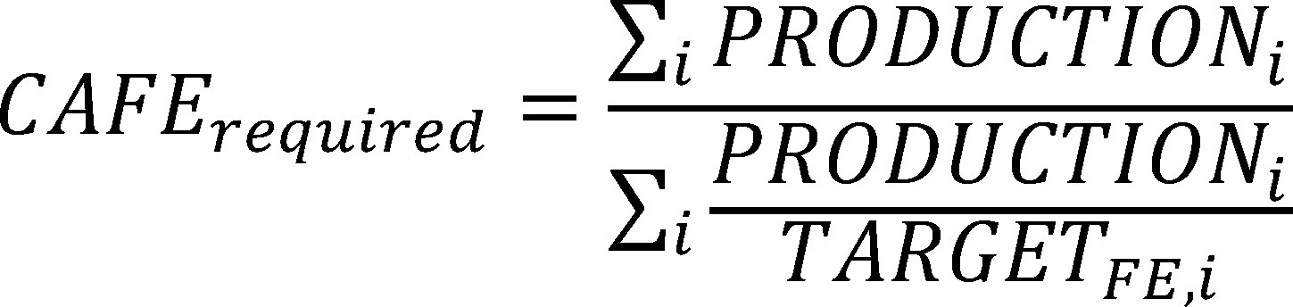
where:
CAFErequired is the CAFE level the fleet is required to achieve,
i refers to specific vehicle model/configurations in the fleet,
PRODUCTIONi is the number of model configuration i produced for sale in the U.S., and
TARGETFE,i the fuel economy target (as defined above) for model configuration i.
Similarly, the required average CO2 level applicable to a given fleet in a given model year is determined by calculating the production-weighted average (not harmonic) of CO2 targets applicable to specific vehicle model configurations in the fleet, as follows:

where:
CO2required is the average CO2 level the fleet is required to achieve,
i refers to specific vehicle model/configurations in the fleet,
PRODUCTIONi is the number of model configuration i produced for sale in the U.S., and
TARGETCO2,i is the CO2 target (as defined above) for model configuration i.
Section VI.A.1 describes the advantages of attribute standards, generally. Section VI.A.2 explains the agencies' specific decision to use vehicle footprint as the attribute over which to vary stringency for past and current rules. Section VI.A.3 discusses the policy considerations in selecting the specific mathematical function. Section VI.A.4 discusses the methodologies used to develop current attribute-based standards, and the agencies' current proposal to continue to do so for MYs 2021-2026. Section VI.A.5 discusses the methodologies used to reconsider the mathematical function for the proposed standards.
1. Why attribute-based standards, and what are the benefits?
Under attribute-based standards, every vehicle model has fuel economy and CO2 targets, the levels of which depend on the level of that vehicle's determining attribute (for the MYs 2021-2026 standards, footprint is the determining attribute, as discussed below). The manufacturer's fleet average CAFE performance is calculated by the harmonic production-weighted average of those targets, as defined below:

Here, i represents a given model [232] in a manufacturer's fleet, Productioni represents the U.S. production of that model, and Targeti represents the target as defined by the attribute-based standards. This means no vehicle is required to meet its target; instead, manufacturers are free to balance improvements however they deem best within (and, given credit transfers, at least partially across) their fleets.
Because CO2 is on a gram per mile basis rather a mile per gallon basis, harmonic averaging is not necessary when calculating required CO2 levels:

The idea is to select the shape of the mathematical function relating the standard to the fuel economy-related attribute to reflect the trade-offs manufacturers face in producing more of that attribute over fuel efficiency (due to technological limits of production and relative demand of each attribute). If the shape captures these trade-offs, every manufacturer is more likely to continue adding fuel-efficient technology across the distribution of the attribute within their fleet, instead of potentially changing the attribute—and other correlated attributes, including fuel economy—as a part of their compliance strategy. Attribute-based standards that achieve this have several advantages.
First, assuming the attribute is a measurement of vehicle size, attribute-based standards help to at least partially reduce the incentive for manufacturers to respond to CAFE and CO2 standards by reducing vehicle size in ways harmful to safety, as compared to “flat,” non-attribute based standards.[233] Larger vehicles, in terms of mass and/or crush space, generally consume more fuel and produce more carbon dioxide emissions, but are also generally better able to protect occupants in a crash.[234] Because each vehicle model has its own target (determined by a size-related attribute), properly fitted attribute-based standards reduce the incentive to build smaller vehicles simply to meet a fleet-wide average, because smaller vehicles are subject to more stringent compliance targets.
Second, attribute-based standards, if properly fitted, provide automakers with more flexibility to respond to consumer preferences than do single-valued standards. As discussed above, a single-valued standard encourages a fleet mix with a larger share of smaller vehicles by creating incentives for manufacturers to use downsizing the average vehicle in their fleet (possibly through fleet mixing) as a compliance strategy, which may result in manufacturers building vehicles for compliance reasons that consumers do not want. Under a size-related, attribute-based standard, reducing the size of the vehicle for compliance's sake is a less-viable strategy because smaller vehicles have more stringent regulatory targets. As a result, the fleet mix under such standards is more likely to reflect aggregate consumer demand for the size-related attribute used to determine vehicle targets.
Third, attribute-based standards provide a more equitable regulatory framework across heterogeneous manufacturers who may each produce different shares of vehicles along attributes correlated with fuel economy.[235] An industry-wide single-value CAFE standard imposes disproportionate cost burden and compliance challenges on manufacturers who produce more vehicles with attributes inherently correlated with lower fuel economy—i.e. manufacturers who produce, on average, larger vehicles. As discussed above, retaining flexibility for manufacturers to produce vehicles which respect heterogeneous market preferences is an important consideration. Since manufacturers may target different markets as a part of their business strategy, ensuring that these manufacturers do not incur a disproportionate share of the regulatory cost burden is an important part of conserving consumer choices within the market.
Industry commenters generally supported attribute-based standards, while other commenters questioned their benefits. IPI argued that preserving the current vehicle mix was not necessarily desirable or necessary for consumer welfare, and suggested that some vehicle downsizing in the fleet might be beneficial both for safety and for compliance.[236] IPI also argued that compliance credit trading would “help smooth out any disproportionate impacts on certain manufacturers” and “ensure that manufacturers with relatively efficient fleets still have an incentive to continue improving fuel economy (in order to generate credits)” [237] Similarly, citing Ito and Sallee, Kathryn Doolittle commented that “. . . Ito and Sallee (2018) have found ABR [“attribute-based regulations”] inefficient in cost when juxtaposed with flat standard with compliance trading.” [238]
The agencies have considered these comments. IPI incorrectly characterizes the agencies' prior statements as claims that it is important to preserve the current vehicle mix. EPA and NHTSA have never claimed, and are not today claiming that it is important to preserve the current fleet mix. The agencies have said, and are today reiterating, that it is reasonable to expect that reducing the tendency of standards to distort the market should reduce at least part of the tendency of standards to reduce consumer welfare. Or, more concisely, it is better to work with the market than against it. Single-value (aka flat) CAFE standards in place from the 1970s through 2010 were clearly distortionary. Recognizing this, the National Academy of Sciences recommended in 2002 that NHTSA adopt attribute-based CAFE standards. NHTSA did so in 2006, for light trucks produced starting MY 2008. As mentioned above, in 2007, Congress codified the requirement for attribute-based passenger car and light truck CAFE standards. Agreeing with this history, premise, and motivation, EPA has also adopted attribute-based CO2 standards. None of this is to say the agencies consider it important to hold fleet mix constant. Rather, the agencies expect that, compared to flat standards, attribute-based standards can allow the market—including fleet mix—to better follow its natural course, and all else equal, consumer acceptance is likely to be greater if the market does so.
The agencies also disagree with comments implying that compliance credit trading can address all of the market distortion that flat standards would entail. Evidence thus far suggests that trading is fragmented, with some manufacturers apparently willing to trade only with some other specific manufacturers. The Ito and Sallee article cited by one commenter is a highly idealized theoretical construction, with the authors noting, inter alia, that their model “assumes perfect competition.” [239] Its findings regarding comparative economic efficiency of flat- and attribute-based standards are, therefore, merely hypothetical, and the agencies find little basis in recent transactions to suggest the compliance credit trading market reflects the authors' idealized assumptions. Even if the agencies did expect credit trading markets to operate as in an idealized textbook example, basing the structure of standards on the presumption of perfect trading would not be appropriate. FCA commented that “. . . when flexibilities are considered while setting targets, they cease to be flexibilities and become simply additional technology mandates,” and the Alliance commented, similarly, that “the Agencies should keep `flexibilities' as optional ways to comply and not unduly assume that each flexibility allows additional stringency of footprint-based standards.” [240] Perhaps recognizing this reality, Congress has barred NHTSA from considering manufacturers' ability to use compliance credits (even credits earned and used by the same OEM, much less credits traded between OEMs). As discussed further in Section VIII.A.2, EPA believes that while credit trading may be a useful flexibility to reduce the overall costs of the program, it is important to set standards in a way that does not rely on credit purchasing availability as a compliance mechanism.
Considering these comments and realities, considering EPCA's requirement for attribute-based CAFE standards, and considering the benefits of regulatory harmonization, the agencies are, again, finalizing attribute-based CAFE and CO2 standards rather than, for either program, finalizing flat standards.
Why footprint as the attribute?
It is important that the CAFE and CO2 standards be set in a way that does not unnecessarily incentivize manufacturers to respond by selling vehicles that are less safe. Vehicle size is highly correlated with vehicle safety—for this reason, it is important to choose an attribute correlated with vehicle size (mass or some dimensional measure). Given this consideration, there are several policy and technical reasons why footprint is considered to be the most appropriate attribute upon which to base the standards, even though other vehicle size attributes (notably, curb weight) are more strongly correlated with fuel economy and tailpipe CO2 emissions.
First, mass is strongly correlated with fuel economy; it takes a certain amount of energy to move a certain amount of mass. Footprint has some positive correlation with frontal surface area, likely a negative correlation with aerodynamics, and therefore fuel economy, but the relationship is less deterministic. Mass and crush space (correlated with footprint) are both important safety considerations. As discussed below and in the accompanying PRIA, NHTSA's research of historical crash data indicates that holding footprint constant, and decreasing the mass of the largest vehicles, will result in a net positive safety impact to drivers overall, while holding footprint constant and decreasing the mass of the smallest vehicles will result in a net decrease in fleetwide safety. Properly fitted footprint-based standards provide little, if any, incentive to build smaller footprint vehicles to meet CAFE and CO2 standards, and therefore help minimize the impact of standards on overall fleet safety.
Second, it is important that the attribute not be easily manipulated in a manner that does not achieve the goals of EPCA or other goals, such as safety. Although weight is more strongly correlated with fuel economy than footprint, there is less risk of artificial manipulation (i.e., changing the attribute(s) to achieve a more favorable target) by increasing footprint under footprint-based standards than there would be by increasing vehicle mass under weight-based standards. It is relatively easy for a manufacturer to add enough weight to a vehicle to decrease its applicable fuel economy target a significant amount, as compared to increasing vehicle footprint, which is a much more complicated change that typically takes place only with a vehicle redesign.
Further, some commenters on the MY 2011 CAFE rulemaking were concerned that there would be greater potential for such manipulation under multi-attribute standards, such as those that also depend on weight, torque, power, towing capability, and/or off-road capability. As discussed in NHTSA's MY 2011 CAFE final rule,[241] it is anticipated that the possibility of manipulation is lowest with footprint-based standards, as opposed to weight-based or multi-attribute-based standards. Specifically, standards that incorporate weight, torque, power, towing capability, and/or off-road capability in addition to footprint would not only be more complex, but by providing degrees of freedom with respect to more easily adjusted attributes, they could make it less certain that the future fleet would actually achieve the projected average fuel economy and CO2 levels. This is not to say that a footprint-based system eliminates manipulation, or that a footprint-based system eliminates the possibility that manufacturers will change vehicles in ways that compromise occupant protection, but footprint-based standards achieve the best balance among affected considerations.
Several stakeholders commented on whether vehicular footprint is the most suitable attribute upon which to base standards. IPI commented that “. . . footprint-based standards may be unnecessary to respect consumer preferences, may negatively impact safety, and may be overall inefficient. Several arguments call into question the footprint-based approach, but a particularly important one is that large vehicles can impose a negative safety externality on other drivers.” [242] IPI commented, further, that the agencies should consider the relative merits of other vehicle attributes, including vehicle fuel type, suggesting that it would be more difficult for manufacturers to manipulate a flatter standard or one “differentiated by fuel type.” [243] Similarly, Michalek and Whitefoot recommended “that the agencies reexamine automaker response to the footprint-based standards to determine if adjustments should be made to avoid inducing increases to vehicle size.” [244]
Conversely, ICCT commented that “the switch to footprint-based CAFE and [CO2] standards has been widely credited with diminishing safety concerns with efficiency standards. Footprint standards encourage larger vehicles with wider track width, which reduces rollovers, and longer wheelbase, which increases the crush space and reduces deceleration forces for both vehicles in a two-vehicle collision.” [245] Similarly, BorgWarner commented that “the use of a footprint standard not only provides greater incentive for mass reduction, but also encourages a larger footprint for a given vehicle mass, thus providing increased safety for a given mass vehicle,” [246] and the Aluminum Association commented footprint based standards drive “fuel-efficiency improvement across all vehicle classes,” “eliminate the incentive to shift fleet volume to smaller cars which has been shown to slightly decrease safety in vehicle-to-vehicle collisions,” and provide “an incentive for reducing weight in the larger vehicles, where weight reduction is of the most benefit for societal safety,” citing Ford's aluminum-intensive F150 pickup truck as an example.[247] NADA urged the agencies to continue basing standards on vehicle footprint, as doing so “serves both to require and allow OEMs to build more fuel-efficient vehicles across the broadest possible light-duty passenger car and truck spectrum,” [248] and UCS commented that footprint-based standards “increase consumer choice, ensuring that the vehicles available for purchase in every vehicle class continue to get more efficient.” [249] Furthermore, regarding concerns that footprint-based standards may be susceptible to manipulation, the Alliance commented that “the data above [from Novation Analytics] shows there are no systemic footprint increases (or any type of target manipulation) occurring.” [250] While FCA's comments supported this Alliance comment, FCA commented further that, lacking some utility-related vehicle attributes such as towing capability, 4-wheel-drive, and ride height, “it is clear the footprint standard does not fully account for pickup truck capability and the components needed such as larger powertrains, greater mass and frontal area,” and requested the agencies “correct LDT standards to reflect the current market preference for capability over efficiency, and introduce mechanisms into the regulation that can adjust for efficiency and capability tradeoffs that footprint standards currently ignore.” [251]
When first electing to adopt footprint-based standards, NHTSA carefully considered other alternatives, including vehicle mass and “shadow” (overall width multiplied by overall length). Compared to both of these other alternatives, footprint is much less susceptible to gaming, because while there is some potential to adjust track width, wheelbase is more expensive to change, at least outside a planned vehicle redesign. EPA agreed with NHTSA's assessment, nothing has changed the relative merits of at least these three potential attributes, and nothing in the evolution of the fleet demonstrates that footprint-based standards are leading manufacturers to increase the footprint of specific vehicle models by more than they would in response to customer demand. Also, even if footprint-based standards are encouraging some increases in vehicle size, NHTSA continues to maintain, and EPA to agree, that such increases should tend to improve overall highway safety rather than degrading it. Regarding FCA's request that the agencies adopt an approach that accounts for a wider range of vehicle attributes related to both vehicle fuel economy and customer-facing vehicle utility, the agencies are concerned that doing so could further complicate already-complex standards and also lead to unintended consequences. For example, it is not currently clear how a multi-attribute approach would appropriately balance emphasis between vehicle attributes (e.g., how much relative fuel consumption should be attributed to, respectively, vehicle footprint, towing capacity, drive type, and ground clearance). Also, basing standards on, in part, ground clearance would encourage manufacturers to increase ride height, potentially increasing the frequency of vehicle rollover crashes. Regarding IPI's recommendation that fuel type be included as a vehicle attribute for attribute-based standards, the agencies note that both CAFE and CO2 standards already account for fuel type in the procedures for measuring fuel economy levels and CO2 emission rates, and for calculating fleet average CAFE and CO2 levels.
Therefore, having considered public comments on the choice of vehicle attributes for CAFE and CO2 standards, the agencies are finalizing standards that, as proposed, are defined in terms of vehicle footprint.
3. What mathematical function should be used to specify footprint-based standards?
In requiring NHTSA to “prescribe by regulation separate average fuel economy standards for passenger and non-passenger automobiles based on 1 or more vehicle attributes related to fuel economy and express each standard in the form of a mathematical function,” EPCA/EISA provides ample discretion regarding not only the selection of the attribute(s), but also regarding the nature of the function. The CAA provides no specific direction regarding CO2 regulation, and EPA has continued to harmonize this aspect of its CO2 regulations with NHTSA's CAFE regulations. The relationship between fuel economy (and CO2 emissions) and footprint, though directionally clear (i.e., fuel economy tends to decrease and CO2 emissions tend to increase with increasing footprint), is theoretically vague, and quantitatively uncertain; in other words, not so precise as to a priori yield only a single possible curve.
The decision of how to specify this mathematical function therefore reflects some amount of judgment. The function can be specified with a view toward achieving different environmental and petroleum reduction goals, encouraging different levels of application of fuel-saving technologies, avoiding any adverse effects on overall highway safety, reducing disparities of manufacturers' compliance burdens, and preserving consumer choice, among other aims. The following are among the specific technical concerns and resultant policy tradeoffs the agencies have considered in selecting the details of specific past and future curve shapes:
- Flatter standards (i.e., curves) increase the risk that both the size of vehicles will be reduced, potentially compromising highway safety, and reducing any utility consumers would have gained from a larger vehicle.
- Steeper footprint-based standards may create incentives to upsize vehicles, potentially oversupplying vehicles of certain footprints beyond what consumers would naturally demand, and thus increasing the possibility that fuel savings and CO2 reduction benefits will be forfeited artificially.
- Given the same industry-wide average required fuel economy or CO2 standard, flatter standards tend to place greater compliance burdens on full-line manufacturers.
- Given the same industry-wide average required fuel economy or CO2standard, dramatically steeper standards tend to place greater compliance burdens on limited-line manufacturers (depending of course, on which vehicles are being produced).
- If cutpoints are adopted, given the same industry-wide average required fuel economy, moving small-vehicle cutpoints to the left (i.e., up in terms of fuel economy, down in terms of CO2 emissions) discourages the introduction of small vehicles, and reduces the incentive to downsize small vehicles in ways that could compromise overall highway safety.
- If cutpoints are adopted, given the same industry-wide average required fuel economy, moving large-vehicle cutpoints to the right (i.e., down in terms of fuel economy, up in terms of CO2 emissions) better accommodates the design requirements of larger vehicles—especially large pickups—and extends the size range over which downsizing is discouraged.
4. What mathematical functions have been used previously, and why?
Notwithstanding the aforementioned discretion under EPCA/EISA, data should inform consideration of potential mathematical functions, but how relevant data is defined and interpreted, and the choice of methodology for fitting a curve to that data, can and should include some consideration of specific policy goals. This section summarizes the methodologies and policy concerns that were considered in developing previous target curves (for a complete discussion see the 2012 FRIA).
As discussed below, the MY 2011 final curves followed a constrained logistic function defined specifically in the final rule.[252] The MYs 2012-2021 final standards and the MYs 2022-2025 augural standards are defined by constrained linear target functions of footprint, as shown below: [253]

Here, Target is the fuel economy target applicable to vehicles of a given footprint in square feet (Footprint). The upper asymptote, a, and the lower asymptote, b, are specified in mpg; the reciprocal of these values represent the lower and upper asymptotes, respectively, when the curve is instead specified in gallons per mile (gpm). The slope, c, and the intercept, d, of the linear portion of the curve are specified as gpm per change in square feet, and gpm, respectively.
The min and max functions will take the minimum and maximum values within their associated parentheses. Thus, the max function will first find the maximum of the fitted line at a given footprint value and the lower asymptote from the perspective of gpm. If the fitted line is below the lower asymptote it is replaced with the floor, which is also the minimum of the floor and the ceiling by definition, so that the target in mpg space will be the reciprocal of the floor in mpg space, or simply, a. If, however, the fitted line is not below the lower asymptote, the fitted value is returned from the max function and the min function takes the minimum value of the upper asymptote (in gpm space) and the fitted line. If the fitted value is below the upper asymptote, it is between the two asymptotes and the fitted value is appropriately returned from the min function, making the overall target in mpg the reciprocal of the fitted line in gpm. If the fitted value is above the upper asymptote, the upper asymptote is returned is returned from the min function, and the overall target in mpg is the reciprocal of the upper asymptote in gpm space, or b.
In this way curves specified as constrained linear functions are specified by the following parameters:
a = upper limit (mpg)
b = lower limit (mpg)
c = slope (gpm per sq.ft.)
d = intercept (gpm)
The slope and intercept are specified as gpm per sq. ft. and gpm instead of mpg per sq. ft. and mpg because fuel consumption and emissions appear roughly linearly related to gallons per mile (the reciprocal of the miles per gallon).
a) NHTSA in MY 2008 and MY 2011 CAFE (Constrained Logistic)
For the MY 2011 CAFE rule, NHTSA estimated fuel economy levels by footprint from the MY 2008 fleet after normalization for differences in technology,[254] but did not make adjustments to reflect other vehicle attributes (e.g., power-to-weight ratios). Starting with the technology-adjusted passenger car and light truck fleets, NHTSA used minimum absolute deviation (MAD) regression without sales weighting to fit a logistic form as a starting point to develop mathematical functions defining the standards. NHTSA then identified footprints at which to apply minimum and maximum values (rather than letting the standards extend without limit) and transposed these functions vertically (i.e., on a gallons-per-mile basis, uniformly downward) to produce the promulgated standards. In the preceding rule, for MYs 2008-2011 light truck standards, NHTSA examined a range of potential functional forms, and concluded that, compared to other considered forms, the constrained logistic form provided the expected and appropriate trend (decreasing fuel economy as footprint increases), but avoided creating “kinks” the agency was concerned would provide distortionary incentives for vehicles with neighboring footprints.[255]
b) MYs 2012-2016 Standards (Constrained Linear)
For the MYs 2012-2016 rule, potential methods for specifying mathematical functions to define fuel economy and CO2 standards were reevaluated. These methods were fit to the same MY 2008 data as the MY 2011 standard. Considering these further specifications, the constrained logistic form, if applied to post-MY 2011 standards, would likely contain a steep mid-section that would provide undue incentive to increase the footprint of midsize passenger cars.[256] A range of methods to fit the curves would have been reasonable, and a minimum absolute deviation (MAD) regression without sales weighting on a technology-adjusted car and light truck fleet was used to fit a linear equation. This equation was used as a starting point to develop mathematical functions defining the standards. Footprints were then identified at which to apply minimum and maximum values (rather than letting the standards extend without limit). Finally, these constrained/piecewise linear functions were transposed vertically (i.e., on a gpm or CO2 basis, uniformly downward) by multiplying the initial curve by a single factor for each MY standard to produce the final attribute-based targets for passenger cars and light trucks described in the final rule.[257] These transformations are typically presented as percentage improvements over a previous MY target curve.
c) MYs 2017 and Beyond Standards (Constrained Linear)
The mathematical functions finalized in 2012 for MYs 2017 and beyond changed somewhat from the functions for the MYs 2012-2016 standards. These changes were made both to address comments from stakeholders, and to consider further some of the technical concerns and policy goals judged more preeminent under the increased uncertainty of the impacts of finalizing and proposing standards for model years further into the future.[258] Recognizing the concerns raised by full-line OEMs, it was concluded that continuing increases in the stringency of the light truck standards would be more feasible if the light truck curve for MYs 2017 and beyond was made steeper than the MY 2016 truck curve and the right (large footprint) cut-point was extended only gradually to larger footprints. To accommodate these considerations, the 2012 final rule finalized the slope fit to the MY 2008 fleet using a sales-weighted, ordinary least-squares regression, using a fleet that had technology applied to make the technology application across the fleet more uniform, and after adjusting the data for the effects of weight-to-footprint. Information from an updated MY 2010 fleet was also considered to support this decision. As the curve was vertically shifted (with fuel economy specified as mpg instead of gpm or CO2 emissions) upwards, the right cutpoint was progressively moved for the light truck curves with successive model years, reaching the final endpoint for MY 2021.
5. Reconsidering the Mathematical Functions for Today's Rulemaking
a) Why is it important to reconsider the mathematical functions?
By shifting the developed curves by a single factor, it is assumed that the underlying relationship of fuel consumption (in gallons per mile) to vehicle footprint does not change significantly from the model year data used to fit the curves to the range of model years for which the shifted curve shape is applied to develop the standards. However, it must be recognized that the relationship between vehicle footprint and fuel economy is not necessarily constant over time; newly developed technologies, changes in consumer demand, and even the curves themselves could influence the observed relationships between the two vehicle characteristics. For example, if certain technologies are more effective or more marketable for certain types of vehicles, their application may not be uniform over the range of vehicle footprints. Further, if market demand has shifted between vehicle types, so that certain vehicles make up a larger share of the fleet, any underlying technological or market restrictions which inform the average shape of the curves could change. That is, changes in the technology or market restrictions themselves, or a mere re-weighting of different vehicles types, could reshape the fit curves.
For the above reasons, the curve shapes were reconsidered in the proposal using the newest available data from MY 2016. With a view toward corroboration through different techniques, a range of descriptive statistical analyses were conducted that do not require underlying engineering models of how fuel economy and footprint might be expected to be related, and a separate analysis that uses vehicle simulation results as the basis to estimate the relationship from a perspective more explicitly informed by engineering theory was conducted as well. Despite changes in the new vehicle fleet both in terms of technologies applied and in market demand, the underlying statistical relationship between footprint and fuel economy has not changed significantly since the MY 2008 fleet used for the 2012 final rule; therefore, EPA and NHTSA proposed to continue to use the curve shapes fit in 2012. The analysis and reasoning supporting this decision follows.
b) What statistical analyses did EPA and NHTSA consider?
In considering how to address the various policy concerns discussed above, data from the MY 2016 fleet was considered, and a number of descriptive statistical analyses (i.e., involving observed fuel economy levels and footprints) using various statistical methods, weighting schemes, and adjustments to the data to make the fleets less technologically heterogeneous were performed. There were several adjustments to the data that were common to all of the statistical analyses considered.
With a view toward isolating the relationship between fuel economy and footprint, the few diesels in the fleet were excluded, as well as the limited number of vehicles with partial or full electric propulsion; when the fleet is normalized so that technology is more homogenous, application of these technologies is not allowed. This is consistent with the methodology used in the 2012 final rule.
The above adjustments were applied to all statistical analyses considered, regardless of the specifics of each of the methods, weights, and technology level of the data, used to view the relationship of vehicle footprint and fuel economy. Table V-1, below, summarizes the different assumptions considered and the key attributes of each. The analysis was performed considering all possible combinations of these assumptions, producing a total of eight footprint curves.

(1) Current Technology Level Curves
The “current technology” level curves exclude diesels and vehicles with electric propulsion, as discussed above, but make no other changes to each model year fleet. Comparing the MY 2016 curves to ones built under the same methodology from previous model year fleets shows whether the observed curve shape has changed significantly over time as standards have become more stringent. Importantly, these curves will include any market forces which make technology application variable over the distribution of footprint. These market forces will not be present in the “maximum technology” level curves: By making technology levels homogenous, this variation is removed. The current technology level curves built using both regression types and both regression weight methodologies from the MY 2008, MY 2010, and MY 2016 fleets, shown in more detail in Chapter 4.4.2.1 of the PRIA, support the curve slopes finalized in the 2012 final rule. The curves built from most methodologies using each fleet generally shift, but remain very similar in slope. This suggests that the relationship of footprint to fuel economy, including both technology and market limits, has not significantly changed.
(2) Maximum Technology Level Curves
As in prior rulemakings, technology differences between vehicle models were considered to be a significant factor producing uncertainty regarding the relationship between fuel consumption and footprint. Noting that attribute-based standards are intended to encourage the application of additional technology to improve fuel efficiency and reduce CO2 emissions across the distribution of footprint in the fleet, approaches were considered in which technology application is simulated for purposes of the curve fitting analysis in order to produce fleets that are less varied in technology content. This approach helps reduce “noise” (i.e., dispersion) in the plot of vehicle footprints and fuel consumption levels and identify a more technology-neutral relationship between footprint and fuel consumption. The results of updated analysis for maximum technology level curves are also shown in Chapter 4.4.2.2 of the PRIA. Especially if vehicles progress over time toward more similar size-specific efficiency, further removing variation in technology application both better isolates the relationship between fuel consumption and footprint and further supports the curve slopes finalized in the 2012 final rule.
c) What other methodologies were considered?
The methods discussed above are descriptive in nature, using statistical analysis to relate observed fuel economy levels to observed footprints for known vehicles. As such, these methods are clearly based on actual data, answering the question “how does fuel economy appear to be related to footprint?” However, being independent of explicit engineering theory, they do not answer the question “how might one expect fuel economy to be related to footprint?” Therefore, as an alternative to the above methods, an alternative methodology was also developed and applied that, using full-vehicle simulation, comes closer to answering the second question, providing a basis either to corroborate answers to the first, or suggest that further investigation could be important.
As discussed in the 2012 final rule, several manufacturers have confidentially shared with the agencies what they described as “physics-based” curves, with each OEM showing significantly different shapes for the footprint-fuel economy relationships. This variation suggests that manufacturers face different curves given the other attributes of the vehicles in their fleets (i.e., performance characteristics) and/or that their curves reflected different levels of technology application. In reconsidering the shapes of the proposed MYs 2021-2026 standards, a similar estimation of physics-based curves leveraging third-party simulation work form Argonne National Laboratories (Argonne) was developed. Estimating physics-based curves better ensures that technology and performance are held constant for all footprints; augmenting a largely statistical analysis with an analysis that more explicitly incorporates engineering theory helps to corroborate that the relationship between fuel economy and footprint is in fact being characterized.
Tractive energy is the amount of energy it will take to move a vehicle.[259] Here, tractive energy effectiveness is defined as the share of the energy content of fuel consumed which is converted into mechanical energy and used to move a vehicle—for internal combustion engine (ICE) vehicles, this will vary with the relative efficiency of specific engines. Data from Argonne simulations suggest that the limits of tractive energy effectiveness are approximately 25 percent for vehicles with internal combustion engines which do not possess integrated starter generator, other hybrid, plug-in, pure electric, or fuel cell technology.
A tractive energy prediction model was also developed to support today's proposal. Given a vehicle's mass, frontal area, aerodynamic drag coefficient, and rolling resistance as inputs, the model will predict the amount of tractive energy required for the vehicle to complete the Federal test cycle. This model was used to predict the tractive energy required for the average vehicle of a given footprint [260] and “body technology package” to complete the cycle. The body technology packages considered are defined in Table V-2, below. Using the absolute tractive energy predicted and tractive energy effectiveness values spanning possible ICE engines, fuel economy values were then estimated for different body technology packages and engine tractive energy effectiveness values.
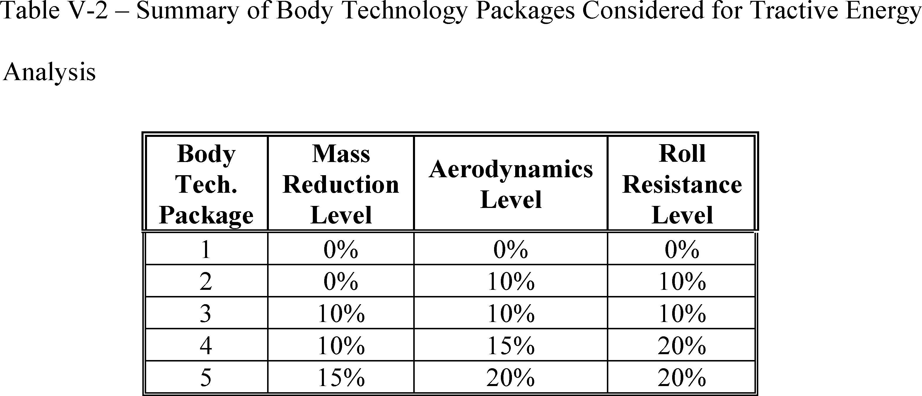
Chapter 6 of the PRIA show the resultant CAFE levels estimated for the vehicle classes Argonne simulated for this analysis, at different footprint values and by vehicle “box.” Pickups are considered 1-box, hatchbacks and minivans are 2-box, and sedans are 3-box. These estimates are compared with the MY 2021 standards finalized in 2012. The general trend of the simulated data points follows the pattern of the previous MY 2021 standards for all technology packages and tractive energy effectiveness values presented in the PRIA. The tractive energy curves are intended to validate the curve shapes against a physics-based alternative, and the analysis suggests that the curve shapes track the physical relationship between fuel economy and tractive energy for different footprint values.
Physical limitations are not the only forces manufacturers face; their success is dependent upon producing vehicles that consumers desire and will purchase. For this reason, in setting future standards, the analysis will continue to consider information from statistical analyses that do not homogenize technology applications in addition to statistical analyses which do, as well as a tractive energy analysis similar to the one presented above.
The relationship between fuel economy and footprint remains directionally discernable but quantitatively uncertain. Nevertheless, each standard must commit to only one function. Approaching the question “how is fuel economy related to footprint” from different directions and applying different approaches has given EPA and NHTSA confidence that the function applied here appropriately and reasonably reflects the relationship between fuel economy and footprint.
The agencies invited comments on this conclusion and the supporting analysis. IPI raised concerns that “. . . several dozen models (mostly subcompacts and sports cars) fall in the 30-40 square feet range, which are all subject to the same standards” and that “manufacturers of these models may have an incentive to decrease footprints as a compliance strategy, since doing so would not trigger more stringent standards.” [261] NHTSA and EPA agree that, all else equal, downsizing the smallest cars (e.g., Chevrolet Spark, Ford Fiesta, Mini Cooper, Mazda MX-5, Porsche 911, Toyota Yaris) would most likely tend to degrade overall highway safety. At the same time, as discussed above, the agencies recognize that small vehicles do appear attractive to some market segments (although obviously the Ford Fiesta and Porsche 911 compete in different segments). Therefore, there is a tension between on one hand, avoiding standards that unduly encourage safety-eroding downsizing and, on the other, avoiding standards that unduly penalize the market for small vehicles. The agencies examined this issue, and note that the market for the smallest vehicles has not evolved at all as estimated in the analysis supporting the 2012 final rule, and attribute this more to fuel prices and consumer demand for larger vehicles than to attribute-based CAFE and CO2 standards. For example, the market for vehicles with footprints less than 40 square foot was about 45 percent smaller in MY 2017 than in MY 2010. The agencies also found that among the smallest vehicle models produced throughout MYs 2010-2017, most have become larger, not smaller. For example, while the Mazda MX-5's footprint decreased by 0.1 square foot (0.3 percent) during that time, the MY 2017 versions of the Mini Cooper, Smart fortwo, Porsche 911, and Toyota Yaris had larger footprints than in MY 2010. With the market for very small vehicles shrinking, and with manufacturers not evidencing a tendency to make the smallest vehicles even smaller, the agencies are satisfied that it would be unwise to change the target functions such that targets never stop becoming more stringent as vehicle footprint becomes ever smaller, because doing so could further impede an already-shrinking market.
B. No-Action Alternative
As in the proposal, the No-Action Alternative applies the augural CAFE and final CO2 targets announced in 2012 for MYs 2021-2025.[262] For MY 2026, this alternative applies the same targets as for MY 2025. The carbon dioxide equivalent of air conditioning refrigerant leakage credits, nitrous oxide, and methane emissions are included for compliance with the EPA standards for all model years under the no-action alternative.[263]

In comments on the DEIS, CBD et al. indicated that it was appropriate for NHTSA to use the augural CAFE standards as the baseline No Action regulatory alternative.[264] However, CARB commented that the baseline regulatory alternative should include CARB's ZEV mandate, in part because EPA must consider “other regulations promulgated by EPA or other government entities,” and, according to CARB, there will be much more vehicle electrification in the future as manufacturers respond to market demand and also work to comply with the ZEV mandate.[265] Similarly, EPA's Science Advisory Board recommended—despite the action taken in the One National Program Action—that the baseline include state ZEV mandates “to be consistent with policies that would prevail in the absence of the rule change.” [266] EPA's Science Advisory Board further recommended including sensitivity analyses with different penetration rates of ZEVs.
On the other hand, arguing for consideration of standards less stringent than those proposed in the NPRM, Walter Kreucher commented that rather than using the augural standards as the baseline, “a better approach would be to assume a clean sheet of paper and start from the existing 2016MY fleet and its associated standards as the baseline using 0%/year increases for both passenger cars and light trucks for MYs 2017-2026.” [267] Similarly, AVE argued that because previously-promulgated standards for MYs 2018-2021 already present a significant challenge that “will likely require almost every automaker to continue using credits for compliance, . . . AVE believes this rulemaking should reset . . . the current compliance baseline for cars and light trucks at MY 2018 . . .” [268] BorgWarner commented similarly that “Beginning in MY 2018, standards should be reset to the levels the industry actually achieved. For MY 2018 and beyond, succeeding model year targets should be set with an annual rate of improvement defined by the slope of improvement the industry has achieved over the last six years. . . . Based on these data, our analysis suggests the most reasonable and logical rate of improvement falls between 2.0% to 2.6% for cars and trucks. Additionally, a single rate of improvement for the combined fleet should be considered.” [269]
The No-Action Alternative represents expectations regarding the world in the absence of a proposal, accounting for applicable laws already in place. Although manufacturers are already making significant use of compliance credits toward compliance with even MY 2017 standards, the agencies are obligated to evaluate regulatory alternatives against the standards already in place through MY 2025. Similarly, even though manufacturers are already producing electric vehicles, EPA and NHTSA appropriately excluded California's ZEV mandate from the No-Action alternative for the NPRM, for several reasons. First, the ZEV mandate is not Federal law; second, as described in the proposal and subsequently finalized in regulatory text, the ZEV mandate is expressly and impliedly preempted by EPCA; third, EPA proposed to withdraw the waiver of CAA preemption in the NPRM and subsequently finalized this withdrawal. Accordingly, the agencies have, therefore, appropriately excluded the ZEV mandate from the No-Action alternative. However, as discussed below, the agencies' analysis does account for the potential that under every regulatory alternative, including the No-Action Alternative, vehicle electrification could increase in the future, especially if batteries become less expensive as gasoline becomes more expensive.
C. Action Alternatives
1. Alternatives in Final Rule
Table V-5 below shows the different alternatives evaluated in today's notice.

With one exception, the alternatives considered in the NPRM included the changes in stringency for the above alternatives. Alternative 3, the preferred alternative, is newly included for today's notice.[270]
Regulations regarding implementation of NEPA requires agencies to “rigorously explore and objectively evaluate all reasonable alternatives, and for alternatives which were eliminated from detailed study, briefly discuss the reasons for their having been eliminated.” [271] This does not amount to a requirement that agencies evaluate the widest conceivable spectrum of alternatives. For example, a State considering adding a single travel lane to a preexisting section of highway would not be required to consider adding three lanes, or to consider dismantling the highway altogether.
Among thousands of individual comments that mentioned the proposed standards very generally, some comments addressed the range and definition of these regulatory alternatives in specific terms, and these specific comments include comments on the stringency, structure, and particular provisions defining the set of regulatory alternatives under consideration.
As discussed throughout today's notice, the agencies have updated and otherwise revised many aspects of the analysis. The agencies have also reconsidered whether the set of alternatives studied in detail should be expanded to include standards less stringent than the proposal's preferred alternative, or to include standards more stringent than the proposal's no-action alternative. On one hand, comments from Walter Kreucher and AVE cited above indicate the agencies should consider relaxing standards below MY 2020 levels, and CEI challenged the agencies' failure to include less-stringent alternatives in the following comments on this question:
DOT failed to consider the possibility of freezing CAFE at an even more lenient standard than currently exists, nor did it consider making its proposed freeze take effect sooner than MY 2020. However, as DOT's own analysis strongly indicates, doing so would lead to even greater benefits and an even greater reduction in CAFE-related deaths and injuries. In short, DOT's failure to consider this possibility is arbitrary and capricious. It has an opportunity to remedy this in its final rule, and it should do so by selecting a standard that is even more lenient than the one it proposed. . . . It should have gone beyond its original set of alternatives and examined less stringent ones as well—until it found one that, for some reason or another, failed to produce greater safety benefits or failed to meet the statutory factors.[272]
On the other hand, a coalition of ten environmental advocacy organizations stated that the agencies should consider alternatives more stringent than those defining the baseline no action alternative, arguing that in light of CEQ guidance and the 2018 IPCC report on climate change, “the increasing danger, increasing urgency, and increasing importance of vehicle emissions all rationally counsel for strengthening emission standards.” [273] CBD et al. observe that “none of these alternatives [considered in the NPRM] increases fuel economy in comparison with the No Action Alternative, none conserves energy . . .” and go on to assert that “none represents maximum feasible CAFE standards.” [274] Similarly, EDF commented that “. . . given its clear statutory directive to maximize fuel savings, NHTSA should have considered a range of alternatives that would be more protective than the existing standards,” [275] and three State agencies in Minnesota commented that “more stringent standards are consistent with EPCA's purpose of energy conservation and the CAA's purpose of reducing harmful air pollutants.” [276] The North Carolina Department of Environmental Quality acknowledged the agencies' determination in the proposal that alternatives beyond the augural standards might be economically impracticable, but nevertheless argued that “alternatives that exceed the stringency of the current standards are consistent with EPCA's purpose” [277] In oral testimony before the agencies, the New York State Attorney General also indicated that the agencies should consider alternatives more stringent than the augural standards.[278] A coalition of States and cities commented that “at a minimum, the existing standards should be left in place, but EPA should also consider whether to make the standards more stringent, not less, just as it has done in prior proposals.” [279] More specifically, through International Mosaic, some individuals commented that the agencies must “fully and publicly consider a few options that require at least a seven annual percent [sic] improvement in vehicle fleet mileage.” [280] In comments on the DEIS, CBD, et al. went further, commenting that “NHTSA's most stringent alternative must be set at no lower than a 9 percent improvement per year.” [281] Most manufacturers who commented on stringency did not identify specific regulatory alternatives that the agencies should consider, although Honda suggested that standards be set to increase in stringency at 5 percent annually for both passenger cars and light trucks throughout model years 2021-2026.[282 283]
The agencies carefully considered these comments to expand the range of stringencies to be evaluated as possible candidates for promulgation. To inform this consideration, the agencies used the CAFE model to examine a progression of stringencies extending outside the range presented in the proposal and draft EIS, and as a point of reference, using a case that reverts to MY 2018 standards starting in MY 2021. Scenarios included in this initial screening exercise ranged as high as increasing annually at 9.5 percent during MYs 2021-2026, reaching average CAFE and CO2 requirements of 66 mpg and 120 g/mi, respectively. Results of this analysis are presented in the following tables and charts. Focusing on MY 2029, the tables show average required and achieved CAFE (as mpg) and CO2 (as g/mi) levels for each scenario, along with average per-vehicle costs (in 2018 dollars, relative to retaining MY 2017 technologies). The proposed (0%/0%), final (1.5%/1.5%), and baseline augural standards are shown in bold type. The charts present the same results on a percentage basis, relative to values shown below for the scenario that reverts to MY 2018 standards starting in MY 2021.
For example, reverting to the MY 2018 CAFE standards starting in MY 2021 yields an average CAFE requirement of 35 mpg by MY 2029, with the industry exceeding that standard by 5 mpg at an average cost of $1,255 relative to MY 2017 technology. Under the augural standards, the MY 2029 requirement increases to 47 mpg, the average compliance margin falls to 1 mpg, and the average cost increases to $2,770. In other words, compared to the scenario that reverts to MY 2018 stringency starting in MY 2021, the augural standards increase stringency by 34 percent (from 35 to 47 mpg), increase average fuel economy by 20 percent (from 40 to 48 mpg), and increase costs by 121 percent (from $1,255 to $2,770).
As indicated in the following two charts, the reality of diminishing returns clearly applies in both directions. On one hand, relaxing stringency below the proposed standards by reverting to MY 2018 or MY 2019 standards reduces average MY 2029 costs by only modest amounts ($54-$121). As discussed in Section VIII, the agencies' updated analysis indicates that the proposed standards would not be maximum feasible considering the EPCA/EISA statutory factors, and would not be appropriate under the CAA after considering the appropriate factors. If further relaxation of standards appeared likely to yield more significant cost reductions, it is conceivable that such savings could outweigh further foregoing of energy and climate benefits. However, this screening analysis does not show dramatic cost reductions. Therefore, the agencies did not include these two less stringent alternatives in the detailed analysis presented in Section VII.
On the other hand, increases in stringency beyond the baseline augural standards show relative costs continuing to accrue much more rapidly than relative CAFE and CO2 improvements. As discussed below in Section VIII, even the no action alternative is already well beyond levels that can be supported under the CAA and EPCA. If further stringency increases appeared likely to yield more significant additional energy and environmental benefits, it is conceivable that these could outweigh these significant additional cost increases. However, this screening analysis shows no dramatic relative acceleration of energy and environmental benefits. Therefore, the agencies did not include stringencies beyond the augural standards in the detailed analysis presented in Section VII.


Specific to model year 2021, some commenters argued that EPCA's lead time requirement prohibits NHTSA from revising CAFE standards for model year 2021.[284] Regarding the revision of standards for model year 2021, NHTSA did consider EPCA's lead time requirement, and determined that while the agency would need to finalize a stringency increase at least 18 months before the beginning of the first affected model year, the agency can finalize a stringency decrease closer (or even after) the beginning of the first affected model year. The agency's reasoning is explained further in Section VIII. Therefore, NHTSA did not change regulatory alternatives to avoid any relaxation of stringency in model year 2021.
The Auto Alliance stated that “the truck increase rate should be no greater than the car rate of increase and should be the `equivalent task' per fleet.” [285] Supporting these Alliance comments, FCA elaborated by commenting that “(1) in MY2017, the latest data we have available, most trucks have a larger gap to standards than cars, and (2) all of the truck segments are challenged because consumers are placing a greater emphasis on capability than fuel economy.” [286] Similarly, Ford commented that “. . . the rates of increase in the stringency of the standards should remain equivalent between passenger cars and light duty trucks.” [287] Other commenters expressed general support for equalizing the rates at which the stringencies of passenger car and light truck standards increase.[288]
For the final rule, the agencies have added an alternative in which stringency for both cars and trucks increases at 1.5 percent. This is consistent with comments received requesting that both fleets' standards increase in stringency by the same amount, and 1.5 percent represents a rate of increase within the range of rates of increase considered in the NPRM.
Throughout the NPRM, the agencies described their consideration as covering a range of alternatives.[289] The preferred alternative for this final rule, an increase in stringency of 1.5 percent for both cars and trucks, falls squarely within the range of alternatives proposed by the agencies.
The NPRM alternatives were bounded on the upper end by the baseline/no action alternative, and the proposed alternative on the lower end (0 percent per year increase in stringency for both cars and trucks). For passenger cars, the agencies considered a range of stringency increases between 0 percent and 2 percent per year for passenger cars, in addition to the baseline/no action alternative. For light trucks, the agencies considered a range of stringency increases between 0 percent and 3 percent per year, in addition to the baseline/no action alternative.
The agencies considered the same range of alternatives for this final rule. As with the proposal, the alternatives for stringency are bounded on the upper end by the baseline/no action alternative and on the lower end by 0 percent per year increases for both passenger cars and light trucks. Consistent with the proposal, for this final rule, the agencies considered stringency increases of between 0 and 2 percent per year for passenger cars and between 0 and 3 percent per year for light trucks, in addition to the baseline/no action alternative.
While it was not specifically modeled in the NPRM, the new preferred alternative of an increase in stringency of 1.5 percent for both cars and trucks was well within the range of alternatives considered. The proposal described the alternatives specifically modeled as options for the agencies, but also gave notice that they did not limit the agencies in selecting from among the range of alternatives under consideration.[290]
The agencies explained in the proposal that they were “taking comment on a wide range of alternatives and have specifically modeled eight alternatives.” [291] As with the proposal, for the final rule, the agencies specifically modeled the upper and lower bounds of the baseline/no action alternative and 0 percent per year stringency increases for both passenger cars and light trucks. In both the proposal and the final rule, the agencies also modeled a stringency increase of 2 percent per year for passenger cars and 3 percent per year for light trucks, as well as a variety of other specific increases between 0 and 2 percent for passenger cars and 0 and 3 percent for light trucks.
The specific alternatives the agencies modeled for the final rule reflect their consideration of public comments. As discussed above, multiple commenters expressed support for equalizing the rates at which the stringencies of passenger car and light truck standards increase. To help the agencies evaluate alternatives that include the same stringency increase for passenger cars and light trucks, three of the seven alternatives (in addition to the baseline/no action alternative) that the agencies specifically modeled for the final rule included the same stringency increase for passenger cars and light trucks. This includes the new preferred alternative of an increase in stringency of 1.5 percent for both cars and trucks. This alternative, and all others specifically modeled for the final rule, falls within the range of alternatives for stringency considered by the agencies in the proposal.
Beyond these stringency provisions discussed in the NPRM, the agencies also sought comment on a number of additional compliance flexibilities for the programs, as discussed in Section IX.
2. Additional Alternatives Suggested by Commenters
Beyond the comments discussed above regarding the shapes of the functions defining fuel economy and CO2 targets, regarding the inclusion of non-CO2 emissions, and regarding the stringencies to be considered, the agencies also received a range of other comments regarding regulatory alternatives.
Some of these additional comments involved how CAFE and CO2 standards compare to one another for any given regulatory alternative. With a view toward maximizing harmonization of the standards, the Alliance, supported by some of its members' individual comments, indicated that “to the degree flexibilities and incentives are not completely aligned between the CAFE and [CO2] programs, there must be an offset in the associated footprint-based targets to account for those differences. Some areas of particular concerns are air conditioning refrigerant credits, and incentives for advanced technology vehicles. The Alliance urges the Agencies to seek harmonization of the standards and flexibilities to the greatest extent possible. . . .” [292]
On the other hand, discussing consideration of compliance credits but making a more general argument, the NYU Institute for Policy Integrity commented that “. . . EPA is not allowed to set lower standards just for the sake of harmonization; to the contrary, full harmonization may be inconsistent with EPA's statutory responsibilities.” [293] Similarly, ACEEE argued that “any consideration of an extension or expansion of credit provisions under the [carbon dioxide] or CAFE standards program should take as a starting point the assumption that the additional credits will allow the stringency of the standards to be increased.” [294]
EPCA's requirement that NHTSA set standards at the maximum feasible levels is separate and “wholly independent” from the CAA's requirement, per Massachusetts v. EPA, that EPA issue regulations addressing pollutants that EPA has determined endanger public health and welfare.[295] Nonetheless, as recognized by the Supreme Court, “there is no reason to think the two agencies cannot both administer their obligations and yet avoid inconsistency.” [296] This conclusion was reached despite the fact that EPCA has a range of very specific requirements about how CAFE standards are to be structured, how manufacturers are to comply, what happens when manufacturers are unable to comply, and how NHTSA is to approach setting standards, and despite the fact that the CAA has virtually no such requirements. This means that while nothing about either EPCA or the CAA, much less the combination of the two, guarantees “harmonization” defining “One National Program,” the agencies are expected to be able to work out the differences.
Since tailpipe CO2 standards are de facto fuel economy standards, the more differences there are between CO2 and CAFE standards and compliance provisions, the more challenging it is for manufacturers to plan year-by-year production that responses to both, and the more difficult it is for affected stakeholders and the general public to understand regulation in this space. Therefore, even if the two statutes, taken together, do not guarantee “full harmonization,” steps toward greater harmonization help with compliance planning and transparency—and meet the expectations set forth by the Supreme Court that the agencies avoid inconsistencies.
The agencies have taken important steps toward doing so. For example, EPA has adopted separate footprint-based CO2 standards for passenger cars and light trucks, and has redefined CAFE calculation procedures to introduce recognition for the application of real-world fuel-saving technology that is not captured with traditional EPA two-cycle compliance testing. Detailed aspects of both sets of standards and corresponding compliance provisions are discussed at length in Section IX. The agencies never set out with the primary goal of achieving “full harmonization,” such that both sets of standards would lead each manufacturer to respond in exactly the same way in every model year.[297] For example, EPA did not adopt the EPCA requirement that domestic passenger car fleets each meet a minimum standard, or the EPCA cap on compliance credit transfers between passenger car fleets. On the other hand, EPA also did not adopt the EPCA civil penalty provisions that have allowed some manufacturers to pay civil penalties as an alternative method of meeting EPCA obligations. These and other differences provide that even if CAFE and CO2 standards are “mathematically” harmonized, for any given manufacturer, the two sets of standards will not be identically burdensome in each model year. Inevitably, one standard will be more challenging than the other, varying over time, between manufacturers, and between fleets. This means manufacturers need to have compliance plans for both sets of standards.
In 2012, recognizing that EPCA provides no clear basis to address HFC, CH4, or N2 O emissions directly, the agencies “offset” CO2 targets from fuel economy targets (after converting the latter to a CO2 basis) by the amounts of credit EPA anticipated manufacturers would, on average, earn in each model years by reducing A/C leakage and adopting refrigerants with reduced GWPs. In 2012, EPA assumed that by 2021, all manufacturers would be earning the maximum available credit, and EPA's analysis assumed that all manufacturers would make progress at the same rate. However, as discussed above, data highlighted in comments by Chemours, Inc., demonstrate that actual manufacturers' adoption of lower-GWP refrigerants thus far ranges widely, with some manufacturers (e.g., Nissan) having taken no such steps to move toward lower-GWP refrigerants, while others (e.g., JLR) have already applied lower-GWP refrigerants to all vehicles produced for sale in the U.S. Therefore, at least in practice, HFC provisions thus far continue to leave a gap (in terms of harmonization) between the two sets of standards. The proposal would have taken the additional step of decoupling provisions regarding HFC (i.e., A/C leakage credits), CH4, and N2 O emissions from CO2 standards, addressing these in separate regulations to be issued in a new proposal. As discussed above, EPA did not finalize this proposal. Accordingly, for the regulatory alternatives considered today, EPA has reinstated offsets of CO2 targets from fuel economy targets, reflecting the assumption that all manufacturers will be earning the maximum available A/C leakage credit by MY 2021.
In addition to general comments on harmonization, the agencies received a range of comments on specific provisions—especially involving “flexibilities”—that may or may not impact harmonization. With a view toward encouraging further electrification, NCAT proposed that EPA extend indefinitely the exclusion of upstream emissions from electricity generation, and also extend and potentially restructure production multipliers for PHEVs, EVs, and FCVs.[298] On the other hand, connecting its comments back to the stringency of standards, NCAT also commented that “. . . expansion of compliance flexibilities in the absence of any requirement to improve [CO2] reduction or fuel economy (as under the agencies' preferred option) could result in an effective deterioration of existing [CO2] and fuel economy performance, as well as little or no effective support for advanced vehicle technology development or deployment.” [299] Global Automakers indicated that the final rule “should include a package of programmatic elements that provide automakers with flexible compliance options that promote the full breadth of vehicle technologies,” such options to include the extension of “advanced technology” production multipliers through MY 2026, the indefinite exclusion of emissions from electricity generation, the extension to passenger cars of credits currently granted for the application of “game changing” technologies (e.g., HEVs) only to full-size pickup trucks, an increase (to 15 g/mi) of the cap on credits for off-cycle technologies, an updated credit “menu” of off-cycle technologies, and easier process for handling applications for off-cycle credits.[300] The Alliance also called for expanded sales multipliers and a permanent exclusion of emissions from electricity generation.[301] Walter Kreucher recommended the agencies consider finalizing the proposed standards but also keeping the augural standards as “voluntary targets” to “provide compliance with the statutes and an aspirational goal for manufacturers.” [302]
The agencies have carefully considered these comments, and have determined that the current suite of “flexibilities” generally provide ample incentive more rapidly to develop and apply advanced technologies and technologies that produce fuel savings and/or CO2 reductions that would otherwise not count toward compliance. The agencies also share some stakeholders' concern that expanding these flexibilities could increase the risk of “gaming” that would make compliance less transparent and would unduly compromise energy and environmental benefits. Nevertheless, as discussed in Section IX, EPA is adopting new multiplier incentives for natural gas vehicles. EPA is also finalizing some changes to procedures for evaluating applications for off-cycle credits, and expects these changes to make this process more accurate and more efficient. Also, EPA is revising its regulations to not require manufacturers to account for upstream emissions associated with electricity use for electric vehicles and plug-in hybrid electric vehicles through model year 2026; compliance will instead be based on tailpipe emissions performance only and not include emissions from electricity generation until model year 2027. As discussed below, even with this change, and even accounting for continued increases in fuel prices and reductions in battery prices, BEVs are projected in this final rule analysis to continue to account for less than 5 percent of new light vehicle sales in the U.S. through model year 2026. To the extent that this projection turns out to reflect reality, this means that the impact of upstream emissions from electricity use on the projected CO2reductions associated with these standards would likely remain small. Regarding comments suggesting that the augural standards should be finalized as “voluntary targets,” the agencies have determined that having such targets exist alongside actual regulatory requirements would be, at best, unnecessary and confusing.
Beyond these additional proposals, some commenters' proposals clearly fell outside authority provided under EPCA or the CAA. Ron Lindsay recommended the agencies “consider postponing the rule changes until the U.S. can establish a legally binding national and international carbon budget and a binding mechanism to adhere to it.” [303] EPCA requires NHTSA to issue standards for MY 2022 by April 1, 2020, and previously-issued EPA regulations commit EPA to revisiting MY 2021-2025 standards on a similar schedule. These statutory and regulatory provisions do not include a basis to delay decisions pending an international negotiation for which prospects and schedules are both unknown.
SCAQMD, supported by Shyam Shukla, indicated that the agencies should consider an alternative that keeps the waiver for California's CO2 standards in place.[304] NCAT and the North Carolina DEQ offered similar comments and CBD, et al. commented that “among the set of more stringent alternatives that NEPA requires the agency to consider, NHTSA must include action alternatives that retain the standards California and other states have lawfully adopted.” [305] As discussed above, the agencies recently issued a final rule addressing the issue of California's authority. NEPA does not require NHTSA to include action alternatives that cannot be lawfully realized.
International Mosiac commented that NHTSA's DEIS “is fatally flawed . . . because it does not consider any market-based alternatives (e.g., a `cap and trade' type option).” [306] While EPCA/EISA does include very specific provisions regarding trading of CAFE compliance credits, the statute provides no authority for a broad-based cap-and-trade program involving other sectors. Similarly, Michalek, et al. wrote that “a more economically efficient approach of, taxing emissions and fuel consumption at socially appropriate levels would allow households to determine whether to reduce fuel consumption and emissions by driving less, by buying a vehicle with more fuel saving technologies, or by buying a smaller vehicle—or, alternatively, not to reduce fuel consumption and emissions at all but rather pay a cost based on the damages they cause. Forcing improvements only through one mechanism (fuel-saving technologies) increases the cost of achieving these outcomes.” [307] While some economists would agree with these comments, Congress has provided no clear authority for NHTSA or EPA to implement either an emissions tax or a broad-based cap-and-trade program in which motor vehicles could participate.
3. Details of Alternatives Considered in Final Rule
a) Alternative 1
Alternative 1 holds the stringency of targets constant and MY 2020 levels through MY 2026.

b) Alternative 2
Alternative 2 increases the stringency of targets annually during MYs 2021-2026 (on a gallon per mile basis, starting from MY 2020) by 0.5 percent for passenger cars and 0.5 percent for light trucks.

c) Alternative 3
Alternative 3; the final standards promulgated today, increases the stringency of targets annually during MYs 2021-2026 (on a gallon per mile basis, starting from MY 2020) by 1.5 percent for passenger cars and 1.5 percent for light trucks.

d) Alternative 4
Alternative 4 increases the stringency of targets annually during MYs 2021-2026 (on a gallon per mile basis, starting from MY 2020) by 1.0 percent for passenger cars and 2.0 percent for light trucks.

e) Alternative 5
Alternative 5 increases the stringency of targets annually during MYs 2022-2026 (on a gallon per mile basis, starting from MY 2021) by 1.0 percent for passenger cars and 2.0 percent for light trucks.

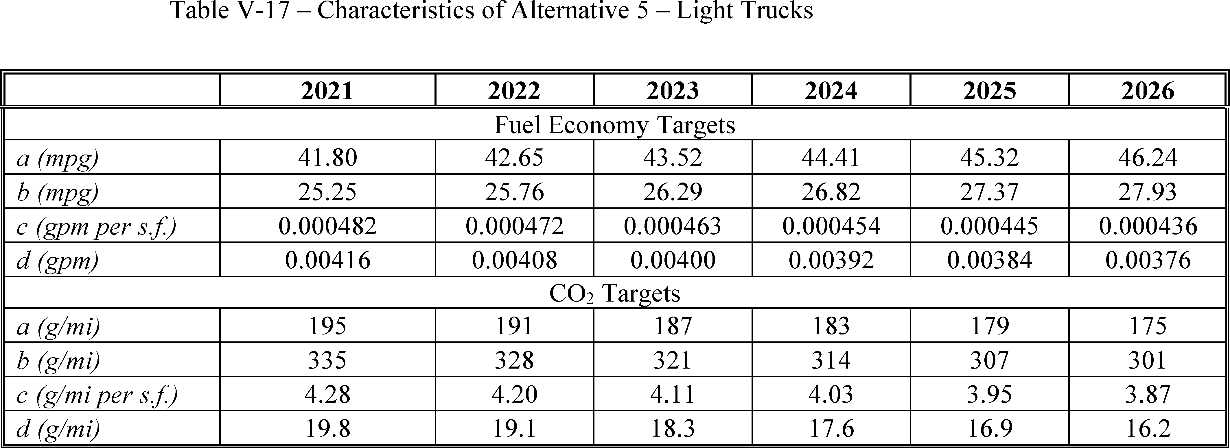
f) Alternative 6
Alternative 6 increases the stringency of targets annually during MYs 2021-2026 (on a gallon per mile basis, starting from MY 2020) by 2.0 percent for passenger cars and 3.0 percent for light trucks.


g) Alternative 7
Alternative 7 increases the stringency of targets annually during MYs 2022-2026 (on a gallon per mile basis, starting from MY 2021) by 2.0 percent for passenger cars and 3.0 percent for light trucks.


EPCA, as amended by EISA, requires that any manufacturer's domestically-manufactured passenger car fleet must meet the greater of either 27.5 mpg on average, or 92 percent of the average fuel economy projected by the Secretary for the combined domestic and non-domestic passenger automobile fleets manufactured for sale in the U.S. by all manufacturers in the model year, which projection shall be published in the Federal Register when the standard for that model year is promulgated in accordance with 49 U.S.C. 32902(b).[308] Any time NHTSA establishes or changes a passenger car standard for a model year, the MDPCS for that model year must also be evaluated or re-evaluated and established accordingly. Thus, this final rule establishes the applicable MDPCS for MYs 2021-2026. Table V-22 lists the minimum domestic passenger car standards.

VI. Analytical Approach as Applied to Regulatory Alternatives
A. Overview of Methods
Like analyses accompanying the NPRM and past CAFE and CAFE/CO2 rulemakings, the analysis supporting today's notice spans a range of technical topics, uses a range of different types of data and estimates, and applies several different types of computer models. The purpose of the analysis is not to determine the standards, but rather to provide information for consideration in doing so. The analysis aims to answer the question “what impacts might each of these regulatory alternatives have?”
Over time, NHTSA's and, more recently, NHTSA's and EPA's analyses have expanded to address an increasingly wide range of types of impacts. Today's analysis involves, among other things, estimating how the application of various combinations of technologies could impact vehicles' costs and fuel economy levels (and CO2 emission rates), estimating how vehicle manufacturers might respond to standards by adding fuel-saving technologies to new vehicles, estimating how changes in new vehicles might impact vehicle sales and operation, and estimating how the combination of these changes might impact national-scale energy consumption, emissions, highway safety, and public health. In addition, the EIS accompanying today's notice addresses impacts on air quality and climate. The analysis of these factors informs and supports both NHTSA's application of the statutory requirements governing the setting of “maximum feasible” fuel-economy standards under EPCA, including, among others, technological feasibility and economic practicability, and EPA's application of the CAA requirements for tailpipe emissions.
Supporting today's analysis, the agencies have brought to bear a variety of different types of data, a few examples of which include fuel economy compliance reports, historical sales and average characteristics of light-duty vehicles, historical economic and demographic measures, historical travel demand and energy prices and consumption, and historical measures of highway safety. Also supporting today's analysis, the agencies have applied several different types of estimates, a few examples of which include projections of the future cost of different fuel-saving technologies, projections of future GDP and the number of households, estimates of the “gap” between “laboratory” and on-road fuel economy, and estimates of the social cost of CO2 emissions and petroleum “price shocks.”
With a view toward transparency, repeatability, and efficiency, the agencies have used a variety of computer models to conduct the majority of today's analysis. For example, the agencies have applied DOE/EIA's National Energy Modeling System (NEMS) to estimate future energy prices, EPA's MOVES model to estimate tailpipe emission rates for ozone precursors and other criteria pollutants, DOE/Argonne's GREET model to estimate emission rates for “upstream” processes (e.g., petroleum refining), and DOE/Argonne's Autonomie simulation tool to estimate the fuel consumption impacts of different potential combinations of fuel-saving technology. In addition, the EIS accompanying today's notice applies photochemical models to estimate air quality impacts, and applies climate models to estimate climate impacts of overall emissions changes.
Use of these different types of data, estimates, and models is discussed further below in the most closely relevant sections. For example, the agencies' use of NEMS is discussed below in the portion of Section VI that addresses the macroeconomic context, which includes fuel prices, and the agencies use of Autonomie is discussed in the portion of Section VI.B.3 that addresses the agencies' approach to estimating the effectiveness of various technologies (in reducing fuel consumption and CO2 emissions).
Providing an integrated means to estimate both vehicle manufacturers' potential responses to CAFE or CO2 standards and, in turn, many of the different potential direct results (e.g., changes in new vehicle costs) and indirect impacts (e.g., changes in rates of fleet turnover) of those responses, the CAFE Model plays a central role in the agencies' analysis supporting today's notice. The agencies used the specific models mentioned above to develop inputs to the CAFE model, such as fuel prices and emission factors. Outputs from the CAFE Model are discussed in Sections VII and VIII of today's notice, and in the accompanying RIA. The EIS accompanying today's notice makes use of the CAFE Model's estimates of changes in total emissions from light-duty vehicles, as well as corresponding changes in upstream emissions. These changes in emissions are included in the set of inputs to the models used to estimate air quality and climate impacts.
The remainder of this overview focuses on the CAFE Model. The purpose of this overview is not to provide a comprehensive technical description of the model,[309] but rather to give an overview of the model's functions, to explain some specific aspects not addressed elsewhere in today's notice, and to discuss some model aspects that were the subject of significant public comment. Some model functions and related comments are addressed in other parts of today's notice. For example, the model's handling of Autonomie-based fuel consumption estimates is addressed in the portion of Section VI.B.3 that discusses the agencies' application of Autonomie. The model documentation accompanying today's notice provides a comprehensive and detailed description of the model's functions, design, inputs, and outputs.
1. Overview of CAFE Model
The basic design of the CAFE Model is as follows: The system first estimates how vehicle manufacturers might respond to a given regulatory scenario, and from that potential compliance solution, the system estimates what impact that response will have on fuel consumption, emissions, and economic externalities. A regulatory scenario involves specification of the form, or shape, of the standards (e.g., flat standards, or linear or logistic attribute-based standards), scope of passenger car and truck regulatory classes, and stringency of the CAFE and CO2 standards for each model year to be analyzed.
Manufacturer compliance simulation and the ensuing effects estimation, collectively referred to as compliance modeling, encompass numerous subsidiary elements. Compliance simulation begins with a detailed user-provided initial forecast of the vehicle models offered for sale during the simulation period. The compliance simulation then attempts to bring each manufacturer into compliance with the standards defined by the regulatory scenario contained within an input file developed by the user. For example, a regulatory scenario may define CAFE or CO2 standards that increase in stringency by 4 percent per year for 5 consecutive years.
The model applies various technologies to different vehicle models in each manufacturer's product line to simulate how each manufacturer might make progress toward compliance with the specified standard. Subject to a variety of user-controlled constraints, the model applies technologies based on their relative cost-effectiveness, as determined by several input assumptions regarding the cost and effectiveness of each technology, the cost of compliance (determined by the change in CAFE or CO2 credits, CAFE-related civil penalties, or value of CO2 credits, depending on the compliance program being evaluated and the effective-cost mode in use), and the value of avoided fuel expenses. For a given manufacturer, the compliance simulation algorithm applies technologies either until the manufacturer runs out of cost-effective technologies, until the manufacturer exhausts all available technologies, or, if the manufacturer is assumed to be willing to pay civil penalties, until paying civil penalties becomes more cost-effective than increasing vehicle fuel economy. At this stage, the system assigns an incurred technology cost and updated fuel economy to each vehicle model, as well as any civil penalties incurred by each manufacturer. This compliance simulation process is repeated for each model year available during the study period.
This point marks the system's transition between compliance simulation and effects calculations. At the conclusion of the compliance simulation for a given regulatory scenario, the system contains multiple copies of the updated fleet of vehicles corresponding to each model year analyzed. For each model year, the vehicles' attributes, such as fuel types (e.g., diesel, electricity), fuel economy values, and curb weights have all been updated to reflect the application of technologies in response to standards throughout the study period. For each vehicle model in each of the model year specific fleets, the system then estimates the following: Lifetime travel, fuel consumption, carbon dioxide and criteria pollutant emissions, the magnitude of various economic externalities related to vehicular travel (e.g., noise), and energy consumption (e.g., the economic costs of short-term increases in petroleum prices). The system then aggregates model-specific results to produce an overall representation of modeling effects for the entire industry.
Different categorization schemes are relevant to different types of effects. For example, while a fully disaggregated fleet is retained for purposes of compliance simulation, vehicles are grouped by type of fuel and regulatory class for the energy, carbon dioxide, criteria pollutant, and safety calculations. Therefore, the system uses model-by-model categorization and accounting when calculating most effects, and aggregates results only as required for efficient reporting.
2. Representation of the Market
As a starting point, the model needs enough information to represent each manufacturer covered by the program. As discussed below in Section VI.B.1, the MY 2017 analysis fleet contains information about each manufacturer's:
- Vehicle models offered for sale—their current (i.e., MY 2017) production volumes, manufacturer suggested retail prices (MSRPs), fuel saving technology content and other attributes (curb weight, drive type, assignment to technology class and regulatory class);
- Production considerations—product cadence of vehicle models (i.e., schedule of model redesigns and “freshenings”), vehicle platform membership, degree of engine and/or transmission sharing (for each model variant) with other vehicles in the fleet; and
- Compliance constraints and flexibilities—preference for full compliance or penalty payment/credit application, willingness to apply additional cost-effective fuel saving technology in excess of regulatory requirements, projected applicable flexible fuel credits, and current credit balance (by model year and regulatory class) in first model year of simulation.
Representation of Fuel-Saving Technologies
The modeling system defines technology pathways for grouping and establishing a logical progression of technologies that can be applied to a vehicle. Technologies that share similar characteristics form cohorts that can be represented and interpreted within the CAFE Model as discrete entities. The following Table VI-1 shows the technologies available within the modeling system used for this final rule. Each technology is discussed in detail below. However, an understanding of the technologies considered and how they are defined in the model (e.g., a 6-speed manual transmission is defined as “MT6”) is helpful for the following explanation of the compliance simulation and the inputs required for that simulation.

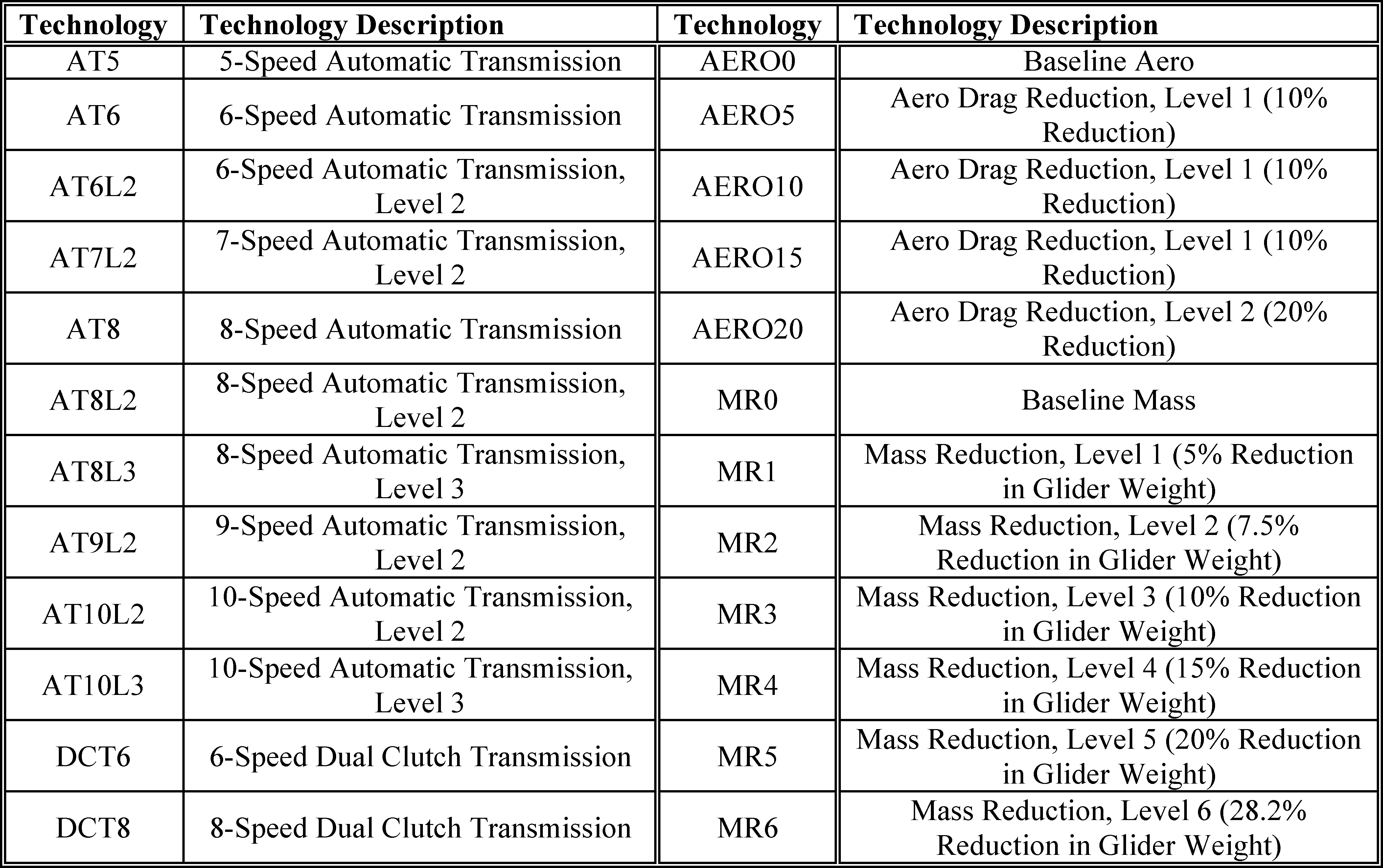
These entities are then laid out into pathways (or paths), which the system uses to define relations of mutual exclusivity between conflicting sets of technologies. For example, as presented in the next section, technologies on the Turbo Engine path are incompatible with those on the HCR Engine or the Diesel Engine paths. As such, whenever a vehicle uses a technology from one pathway (e.g., turbo), the modeling system immediately disables the incompatible technologies from one or more of the other pathways (e.g., HCR and diesel).
In addition, each path designates the direction in which vehicles are allowed to advance as the modeling system evaluates specific technologies for application. Enforcing this directionality within the model ensures that a vehicle that uses a more advanced or more efficient technology (e.g., AT8) is not allowed to “downgrade” to a less efficient option (e.g., AT5). Visually, as portrayed in the charts in the sections that follow, this is represented by an arrow leading from a preceding technology to a succeeding one, where vehicles begin at the root of each path, and traverse to each successor technology in the direction of the arrows.
The modeling system incorporates twenty technology pathways for evaluation as shown below. Similar to individual technologies, each path carries an intrinsic application level that denotes the scope of applicability of all technologies present within that path, and whether the pathway is evaluated on one vehicle at a time, or on a collection of vehicles that share a common platform, engine, or transmission.

Even though technology pathways outline a logical progression between related technologies, all technologies available to the system are evaluated concurrently and independently of each other. Once all technologies have been examined, the model selects a solution deemed to be most cost-effective for application on a vehicle. If the modeling system applies a technology that resides later in the pathway, it will subsequently disable all preceding technologies from further consideration to prevent a vehicle from potentially downgrading to a less advanced option. Consequently, the system skips any technology that is already present on a vehicle (either those that were available on a vehicle from the input fleet or those that were previously applied by the model). This “parallel technology” approach, unlike the “parallel path” methodology utilized in the preceding versions of the model, allows the system always to consider the entire set of available technologies instead of foregoing the application of potentially more cost-effective options that happen to reside further down the pathway.[310] This revised approach addresses comments summarized below, and allows the system to analyze all available technology options concurrently and independently of one other without having to first apply one or more “predecessor” technologies. For example, if model inputs are such that a 7-speed transmission is cost-effective, but not as cost-effective as an 8-speed transmission, the revised approach enables the model to skip over the 7-speed transmission entirely, whereas the NPRM version of the model might first apply the 7-speed transmission and then consider whether to proceed immediately to the 8-speed transmission. As such, the model's choices for evaluation of new technology solutions becomes slightly less restrictive, allowing it immediately to consider and apply more advanced options, and increasing the likelihood that the a globally optimum solution is selected.
Some commenters supported the agencies' use of such pathways in the simulation of manufacturers' potential application of technologies. As one of a dozen examples of CAFE model design elements that lead to the transparent representation of real-world factors, the Alliance highlighted “recognition of the need for manufacturers to follow `technology' pathways that retain capital and implementation expertise, such as specializing in one type of engine or transmission instead of following an unconstrained optimization that would cause manufacturers to leap to unrelated technologies and show overly optimistic costs and benefits.” [311] Similarly, Toyota commented that “the inertia of capital investments and engineering expertise dedicated to one compliance technology or set of technologies makes it unreasonable for manufacturers to immediately switch to another technology path.” [312]
Other commenters cited the use of technology pathways as inherently overly restrictive. For example, as an example of “arbitrary model constraints,” a coalition of commenters cited the fact the model “prohibit[s] manufacturers from switching vehicle technology pathways.” [313] Also, EDF, UCS, and CARB cited the combination of technology pathways, decision making criteria, and model inputs as producing unrealistic results.[314] Regarding the technology pathways, specifically, EDF's consultant argued that the technology paths are not transparent, and cited the potential that specific paths may not necessarily be arranged in progression from least to most cost-effective—that “NHTSA ignores the cost of the technology when developing this list.” [315] Relatedly, as EDF's consultant commented:
[T]he Volpe Model is not designed to look backwards along its technology paths. Thus, the opportunity to recover the expenditure of inefficient technology is missed. NHTSA might argue that a manufacturer will not invest in 10-speed transmissions, for example, and then return to an older design. Whether or not this is true in real life, such a view would put too much stake in the Volpe Model projections. The model simply projects what could be done, not what will be. Anyone examining the progression of technology and noting the reversion of transmission technology could easily modify the model inputs to avoid this. Also, if NHTSA evaluated combinations of technologies prior to entering them in the model piecemeal, it would automatically avoid such apparent problems.[316]
The agencies also received additional public comments on specific paths and specific interactions between paths (e.g., involving engines and hybridization). These comments are addressed below.
The agencies have carefully considered these comments and the approach summarized below reflects some corresponding revision. As mentioned above, the CAFE model now approaches the technology paths in a such way that, faced with two cost-effective technologies on the same path, the model can proceed directly to the more advanced technology if that technology is the more cost effective of the two.
However, the agencies reject assertions that the model's use of technology paths is not transparent. The agencies provided extensive explanatory text, figures, model documentation, and model source code specifically addressing these paths (and other model features). This transparency appears evident in that commenters (sometimes while claiming that a specific feature of the model is not transparent) presented analytical results involving changes to corresponding inputs that required a detailed understanding of that feature's operation.
Regarding comments that the technology paths should be arranged in order of cost-effectiveness, the agencies note that such comments presume, without merit, that costs, fuel consumption impacts, and other inputs (e.g., fuel prices) that logically impact manufacturers' decision-making are not subject to uncertainty. These inputs are all subject to uncertainty, and the CAFE Model's arrangement of technologies into several paths is responsive to these uncertainties. Nevertheless, the agencies maintain that some technologies do reflect a higher level of advancement than others (e.g., 10-speed transmissions vs. 5-speed transmissions), and while manufacturers may, in practice, occasionally revert to less advanced technologies, it is appropriate and reasonable to conduct the agencies' analysis in a manner that assumes manufacturers will continue to make forward progress. As observed by EDF's consultant's remarks, the CAFE Model “simply projects what could be done, not what will be.” While no model, much less any model relying on information that can be made publicly available, can hope to represent precisely each manufacturers' actual detailed constrains related to product development and planning, such constraints are real and important. The agencies agree that the CAFE Model's representation of such constraints—including the Model's use of technology paths—provides a reasonable means of accounting for them.
4. Compliance Simulation
The CAFE model provides a way of estimating how vehicle manufacturers could attempt to comply with a given CAFE standard by adding technology to fleets that the agencies anticipate they will produce in future model years. This exercise constitutes a simulation of manufacturers' decisions regarding compliance with CAFE or CO2 standards.
This compliance simulation begins with the following inputs: (a) The analysis fleet of vehicles from model year 2017 discussed below in Section VI.B.1, (b) fuel economy improving technology estimates discussed below in Section VI.C, (c) economic inputs discussed below in Section VI.D, and (d) inputs defining baseline and potential new CAFE or CO2 standards discussed above in Section V. For each manufacturer, the model applies technologies in both a logical sequence and a cost-optimizing strategy in order to identify a set of technologies the manufacturer could apply in response to new CAFE or CO2 standards. The model applies technologies to each of the projected individual vehicles in a manufacturer's fleet, considering the combined effect of regulatory and market incentives while attempting to account for manufacturers' production constraints. Depending on how the model is exercised, it will apply technology until one of the following occurs:
(1) The manufacturer's fleet achieves compliance [317] with the applicable standard and adding additional technology in the current model year would be attractive neither in terms of stand-alone (i.e., absent regulatory need) cost-effectiveness nor in terms of facilitating compliance in future model years;
(2) The manufacturer “exhausts” available technologies; [318] or
(3) For manufacturers assumed to be willing to pay civil penalties (in the CAFE program), the manufacturer reaches the point at which doing so would be more cost-effective (from the manufacturer's perspective) than adding further technology.
The model accounts explicitly for each model year, applying technologies when vehicles are scheduled to be redesigned or freshened and carrying forward technologies between model years once they are applied (until, if applicable, they are superseded by other technologies). The model then uses these simulated manufacturer fleets to generate both a representation of the U.S. auto industry and to modify a representation of the entire light-duty registered vehicle population. From these fleets, the model estimates changes in physical quantities (gallons of fuel, pollutant emissions, traffic fatalities, etc.) and calculates the relative costs and benefits of regulatory alternatives under consideration.
The CAFE model accounts explicitly for each model year, in turn, because manufacturers actually “carry forward” most technologies between model years, tending to concentrate the application of new technology to vehicle redesigns or mid-cycle “freshenings,” and design cycles vary widely among manufacturers and specific products. Comments by manufacturers and model peer reviewers strongly support explicit year-by-year simulation. Year-by-year accounting also enables accounting for credit banking (i.e., carry-forward), as discussed above, and at least four environmental organizations recently submitted comments urging the agencies to consider such credits, citing NHTSA's 2016 results showing impacts of carried-forward credits.[319] Moreover, EPCA/EISA requires that NHTSA make a year-by-year determination of the appropriate level of stringency and then set the standard at that level, while ensuring ratable increases in average fuel economy through MY 2020. The multi-year planning capability, simulation of “market-driven overcompliance,” and EPCA credit mechanisms (again, for purposes of modeling the CAFE program) increase the model's ability to simulate manufacturers' real-world behavior, accounting for the fact that manufacturers will seek out compliance paths for several model years at a time, while accommodating the year-by-year requirement. This same multi-year planning structure is used to simulate responses to standards defined in grams CO2/mile, and utilizing the set of specific credit provisions defined under EPA's program.
After the light-duty rulemaking analysis accompanying the 2012 final rule that finalized NHTSA's standards through MY 2021, NHTSA began work on changes to the CAFE model with the intention of better reflecting constraints of product planning and cadence for which previous analyses did not account. This involves accounting for expected future schedules for redesigning and “freshening” vehicle models, and accounting for the fact that a given engine or transmission is often shared among more than one vehicle model, and a given vehicle production platform often includes more than one vehicle model. These real product planning considerations are explained below.
Like earlier versions, the current CAFE model provides the capability for integrated analysis spanning different regulatory classes, accounting both for standards that apply separately to different classes and for interactions between regulatory classes. Light vehicle CAFE and CO2 standards are specified separately for passenger cars and light trucks. However, there is considerable sharing between these two regulatory classes, where a single engine, transmission, or platform can appear in both the passenger car and light truck regulatory class. For example, some sport-utility vehicles are offered in 2WD versions (classified as passenger cars for compliance purposes) and 4WD versions (classified as light trucks for compliance purposes). Integrated analysis of manufacturers' passenger car and light truck fleets provides the ability to account for such sharing and reduces the likelihood of finding solutions that could involve introducing impractical and unrealistic levels of complexity in manufacturers' product lines. In addition, integrated fleet analysis provides the ability to simulate the potential that manufacturers could earn CAFE and CO2 credits by over complying with the standard in one fleet and use those credits toward compliance with the standard in another fleet (i.e., to simulate credit transfers between regulatory classes).[320]
The CAFE model also accounts for EPCA's requirement that compliance be determined separately for fleets of domestic passenger cars and fleets of imported passenger cars. The model accounts for all three CAFE regulatory classes simultaneously (i.e., in an integrated way) yet separately: Domestic passenger cars, imported passenger cars, and light trucks. The model further accounts for two related specific statutory requirements specifically involving this distinction between domestic and imported passenger cars. First, EPCA/EISA requires that any given fleet of domestic passenger cars meet a minimum standard, irrespective of any available compliance credits. Second, EPCA/EISA requires compliance with the standards applicable to the domestic passenger car fleet without regard to traded or transferred credits.[321]
However, the CAA has no such limitation regarding compliance by domestic and imported vehicles; EPA did not adopt provisions similar to the aforementioned EPCA/EISA requirements and is not doing so today. Therefore, the CAFE model determines compliance for manufacturers' overall passenger car and light truck fleets for EPA's program.
Each manufacturer's regulatory requirement represents the production-weighted harmonic mean of their vehicle's targets in each regulated fleet. This means that no individual vehicle has a “standard,” merely a target, and each manufacturer is free to identify a compliance strategy that makes the most sense given its unique combination of vehicle models, consumers, and competitive position in the various market segments. As the CAFE model provides flexibility when defining a set of regulatory standards, each manufacturer's requirement is dynamically defined based on the specification of the standards for any simulation and the distribution of footprints within each fleet.
Given this information, the model attempts to apply technology to each manufacturer's fleet in a manner that, given product planning and engineering-related considerations, optimizes the selected cost-related metric. The metric supported by the NPRM version of the model is termed “effective cost.” The effective cost captures more than the incremental cost of a given technology; it represents the difference between their incremental cost and the value of fuel savings to a potential buyer over the first 30 months of ownership.[322] In addition to the technology cost and fuel savings, the effective cost also includes the change in CAFE civil penalties from applying a given technology and any estimated welfare losses associated with the technology (e.g., earlier versions of the CAFE model simulated low-range electric vehicles that produced a welfare loss to buyers who valued standard operating ranges between re-fueling events). Comments on this metric are discussed below, as are model changes responding to these comments.
This construction allows the model to choose technologies that both improve a manufacturer's regulatory compliance position and are most likely to be attractive to its consumers. This also means that different assumptions about future fuel prices will produce different rankings of technologies when the model evaluates available technologies for application. For example, in a high fuel price regime, an expensive but very efficient technology may look attractive to manufacturers because the value of the fuel savings is sufficiently high both to counteract the higher cost of the technology and, implicitly, to satisfy consumer demand to balance price increases with reductions in operating cost.
In general, the model adds technology for several reasons but checks these sequentially. The model then applies any “forced” technologies. Currently, only variable valve timing (VVT) is forced to be applied to vehicles at redesign since it is the root of the engine path and the reference point for all future engine technology applications.[323] The model next applies any inherited technologies that were applied to a leader vehicle on the same vehicle platform and carried forward into future model years where follower vehicles (on the shared system) are freshened or redesigned (and thus eligible to receive the updated version of the shared component). In practice, very few vehicle models enter without VVT, so inheritance is typically the first step in the compliance loop. Next, the model evaluates the manufacturer's compliance status, applying all cost-effective technologies regardless of compliance status.[324] Then the model applies expiring overcompliance credits (if allowed to do so under the perspective of either the “unconstrained” or “standard setting” analysis, for CAFE purposes).[325] At this point, the model checks the manufacturer's compliance status again. If the manufacturer is still not compliant (and is unwilling to pay civil penalties, again for CAFE modeling), the model will add technologies that are not cost-effective until the manufacturer reaches compliance. If the manufacturer exhausts opportunities to comply with the standard by improving fuel economy/reducing emissions (typically due to a limited percentage of its fleet being redesigned in that year), the model will apply banked CAFE or CO2 credits to offset the remaining deficit. If no credits exist to offset the remaining deficit, the model will reach back in time to alter technology solutions in earlier model years.
The CAFE model implements multi-year planning by looking back, rather than forward. When a manufacturer is unable to comply through cost-effective (i.e., producing effective cost values less than zero) technology improvements or credit application in a given year, the model will “reach back” to earlier years and apply the most cost-effective technologies that were not applied at that time and then carry those technologies forward into the future and re-evaluate the manufacturer's compliance position. The model repeats this process until compliance in the current year is achieved, dynamically rebuilding previous model year fleets and carrying them forward into the future, and accumulating CAFE or CO2 credits from over-compliance with the standard wherever appropriate.
In a given model year, the model determines applicability of each technology to each vehicle platform, model, engine, and transmission. The compliance simulation algorithm begins the process of applying technologies based on the CAFE or CO2 standards specified during the current model year. This involves repeatedly evaluating the degree of noncompliance, identifying the next “best” technology (ranked by the effective cost discussed earlier) available on each of the parallel technology paths described above and applying the best of these. The algorithm combines some of the pathways, evaluating them sequentially instead of in parallel, to ensure appropriate incremental progression of technologies.
The algorithm first finds the best next applicable technology in each of the technology pathways and then selects the best among these. For CAFE purposes, the model applies the technology to the affected vehicles if a manufacturer is either unwilling to pay penalties or if applying the technology is more cost-effective than paying penalties. Afterwards, the algorithm reevaluates the manufacturer's degree of noncompliance and continues application of technology. Once a manufacturer reaches compliance (i.e., the manufacturer would no longer need to pay penalties), the algorithm proceeds to apply any additional technology determined to be cost-effective (as discussed above). Conversely, if a manufacturer is assumed to prefer to pay penalties, the algorithm only applies technology up to the point where doing so is less costly than paying penalties. The algorithm stops applying additional technology to this manufacturer's products once no more cost-effective solutions are encountered. This process is repeated for each manufacturer present in the input fleet. It is then repeated for each model year. Once all model years have been processed, the compliance simulation algorithm concludes. The process for CO2 standard compliance simulation is similar, but without the option of penalty payment, such that technologies are applied until compliance (accounting for any modeled application of credits) is achieved. For both CAFE and CO2 standards, the model also applies any additional (i.e., beyond required for compliance) technology that “pays back” within a specified period (for the NPRM and today's analysis, 30 months).
Some commenters argued that the CAFE model applies constraints that excessively limit options manufacturers have to add technology, causing the model to overestimate costs to achieve a given level of improvement.[326] Some of these commenters further argued that the agencies should assume greater potential to apply technologies that contribute to compliance by improving air conditioner efficiency or otherwise reducing “off cycle” fuel consumption and CO2 emissions.[327] Other commenters argued that such constraints, while warranting some refinements, help the model to simulate manufacturers' decision making realistically and to estimate technology effectiveness and costs reasonably.[328 329]
Some commenters questioned the “effective cost” metric the model uses to decide among available options, claiming that the metric also causes the model to avoid selection of pathways that are not always economically optimal.[330] One of these commenters recommended the agencies modify the effective cost metric for CO2 compliance by removing the term placing a monetary value on progress toward compliance, and instead dividing the remaining net cost (i.e., the increase in technology costs minus a portion of the fuel outlays expected to be avoided) by the additional CO2 credits earned.[331] Another of these commenters claimed on one hand, that the effective cost metric “does not include a measurement of the technology's reduction in fuel consumption or CO2 emissions” and, on the other, that the metric inappropriately places a value on avoided fuel consumption.[332]
One commenter claimed that the model inappropriately allows earned credits (including CO2 program credits for which EPA has granted a one-time exemption from carry-forward limits) to expire while also showing undue degrees overcompliance with standards, and further proposed that the model be modified to simulate both credit “carry back” (aka “borrowing”) and credit trading between manufacturers.[333]
In addition, some commenters indicated that the agencies' analysis (impliedly, its modeling) should account for some States' mandates that manufacturers sell minimum quantities of “Zero Emission Vehicles” (ZEVs).[334 335]
Regarding the model's representation of engineering and product planning constraints, the agencies maintain that having such constraints produces more realistic potential (as mentioned above, not “predicted”) pathways forward from manufacturers' current fleets than would be the case were these constraints removed. For example, while manufacturers' product plans are protected as confidential business information (CBI), some manufacturers' public comments demonstrate year-by-year balancing such as the CAFE model emulates.[336] Also, even manufacturers that have invested in technologies such as hybrid electric powertrains and Atkinson cycle engines have commented that a manufacturers' past investments will constrain the pathways it can practicably take.[337] Therefore, the agencies have retained the model's basic structural constraints, have updated and expanded the model's technology paths (and, as discussed, the model's logic for approaching these paths), and have updated inputs defining the range of manufacturer-, technology-, and product-specific constraints. These updates are discussed below at greater length.
The agencies have also reconsidered opportunities manufacturers may have to expand the application of technologies that contribute to compliance by improving air conditioner efficiency or otherwise reducing “off cycle” fuel consumption and CO2 emissions, or to earn credit toward CO2 compliance by using refrigerants with lower global warming potential (GWP) or reducing the potential for refrigerant leaks. The version of the model used for the proposal accommodates inputs that, for each of these adjustments or credits, applies the same value to every model year. The agencies have revised the model to accommodate inputs that specify the degree of adjustment or credit separately for each model year, and have applied inputs that assume manufacturers will increase application of these improvements to the highest levels reported within the industry.
Regarding comments on the effective cost metric the model uses to compare and select among available options to add technology, the agencies have considered changes such as those mentioned above. Given the myriad of factors that manufacturers can consider, any weighing to be conducted using publicly-available information will constitute a simplified representation. Nevertheless, within the model's context, it is obvious that any weighing of options should, at a minimum, consider some measure of each option's costs and benefits. Since this aspect of the model involves simulating manufacturers' decisions, it is also clearly appropriate that these costs and benefits be considered from a manufacturer perspective rather than a social perspective.
The effective cost metric used for the NPRM version of the model represents the cost of a given option as the cost to apply a given technology to a given set of vehicles, and represents the benefit of the same option as the extent to which the manufacturer might expect buyers would be willing to pay for fuel economy (as represented by a portion of the projected fuel savings), combined with any reduction in CAFE civil penalties that the manufacturer might ultimately need to pass along to buyers. The reduction in CAFE civil penalties places a value on progress made toward compliance with CAFE standards. The CAA provides no direction regarding CO2 standards, so the model accepts inputs specifying an analogous basis for valuing changes in the quantity of CO2 credits earned from (or required by) a manufacturer's fleet. Because each of these three components (technology cost, fuel benefit, and compliance benefit) is expressed in dollars, subtracting benefits from costs produces a net cost, and after dividing net costs by the number of affected vehicles, it is logical to, at each step, select the option that produces the most negative net unit cost. This approach can be interpreted as maximizing net benefits (to the manufacturer).
As an alternative, the agencies considered a simpler metric that considers only the cost of the option and the extent to which the option increases the quantity of earned credits, and does not require input assumptions regarding how to value progress toward compliance. Such a metric is expressed in dollars per ton or dollars per gallon such that seeking options that produce the smallest (positive) values can be interpreted as maximizing cost effectiveness (of progress toward compliance). However, simply comparing technology costs to corresponding compliance improvements would implicitly assume that manufacturers do not respond at all to fuel prices. This assumption is clearly unrealistic. For example, if diesel fuel costs $5 per gallon and gasoline costs $2 per gallon, manufacturers will be reluctant to respond to stringent CAFE or CO2 standards by replacing gasoline engines with diesel engines. Manufacturers' comments credibly assert that fuel prices matter, and in the agencies' judgment, simulations of decisions between available options should continue to account for avoided fuel outlays.
On the other hand, while any metric should incorporate some measure of progress toward compliance, it is not obvious that this progress must be expressed in monetary terms. While the CAFE civil penalty provisions provide a logical basis for doing so with respect to CAFE, the recently-introduced (through EISA) option to trade credit between manufacturers adds an alternative basis that is undefined and uncertain, in part because terms of past trades are not known to the agencies. Also, as mentioned above, EPCA/EISA's civil penalty provisions are not applicable to noncompliance with CO2 standards.
Therefore, for the purpose of selecting among available options to add technology, the agencies consider it reasonable to use the degree of compliance improvement in “raw” (i.e., not monetized) form, and to divide net costs (i.e., technology costs minus a portion of expected avoided fuel outlays) by this improvement. Under a range of side-by-side tests, this change to the effective cost metric most frequently produced lower overall estimates of compliance costs. However, differences vary among manufacturers, model years, and regulatory alternatives, and also depend on other model inputs. For example, at high fuel prices, the new metric tends to select more expensive pathways than the NPRM's metric, and with the new metric, a case simulating “perfect trading” of CO2 compliance credits tends to show such trading increasing compliance costs rather than, as expected, decreasing such costs.
The version of the model used for the proposal simulates the potential that, for a given fleet in a given model year, a manufacturer might be able to use credits from an earlier model year or a different fleet. This version of the model did not explicitly simulate the potential that, for a given fleet in a given model year, a manufacturer might be to use credits from a future model year or a different manufacturer. However, the agencies did apply model inputs that reflected assumptions regarding possible trading of credits actually earned prior to model year 2016 (the earliest represented in detail in the agencies' analysis), and the agencies did examine a case (included in the sensitivity analysis) involving hypothetical “perfect” trading of CO2 credits among manufacturers by treating the industry as a single “manufacturer.” Although past versions of the CAFE Model had included code under development with a view toward eventually simulating one or both of these provisions, this code had never proceeded beyond preliminary experimentation, and had never been the focus of peer reviews or application in published analyses.
Nevertheless, the agencies considered expanding the model to simulate credit “carry back” (or “borrowing”) and trading (explicitly, rather than in an idealized hypothetical way). The agencies closely examined the corresponding model revisions proposed by UCS and determined that such methods would not produce repeatable results. This is because the approach proposed by UCS “randomly swaps items in list to minimize trading bias.” [338]
Even if such revisions could be modified to produce non-random results, including credit banking and trading would introduce highly speculative elements into the agencies' analysis. While manufacturers have occasionally indicated plans to carry back credits from future model years, those plans have sometimes backfired when projected credits have failed to materialize, e.g., by misjudging consumer demand for more efficient vehicles. In the agencies' judgment, it would be inappropriate to set standards based on an analysis that relies on the type of borrowing that has been known to fail. To rely also on credit trading during the model years included in the analysis would compound this undue speculation. For example, including credit borrowing and trading throughout the analysis, as some commenters proposed, would lead to an analysis that depends on the potential that, in order to comply with the MY 2022 standard for light trucks, FCA could use credits it expects to be able to buy from another manufacturer in MY 2025. Even if the agencies' analysis had knowledge of and made use of manufacturers' actual product plans, expectations about the ability to borrow others' unearned credits would necessarily be considered risky and unreliable. Within an analysis that, to provide for public disclosure, extrapolates forward many years from the most recent observed fleet, such transactions would add an unreasonable level of speculation. Therefore, the agencies have declined to introduce credit borrowing and trading into the model's logic.
The analysis presented in the proposal applied inputs reflecting potential application of credits earned earlier than the first year modeled explicitly. However, as observed by some commenters, those inputs did not fully account for the one-time exemption from the 5-year limit on the extent to which manufacturers may carry forward CO2 credits. The agencies have updated the analysis fleet to MY 2017 and, in doing so, have updated inputs specifying how credits earned to MY 2017 might be applied. These updates implement a reasonably full accounting of these “legacy” credits, including of the one-time exemption from the credit life limit.
As mentioned above, some commenters also indicated that the model is unrealistically “reluctant” to apply credits carried forward from early model years. As explained in the proposal and in the model documentation, the model's application of carried-forward credits is partially controlled by model inputs, which, for the proposal, were set to assume that manufacturers would tend to retain credits as long as possible. This assumption is entirely consistent with manufacturers' past practice and logical in a context wherein the stringency of standards is generally increasing over time. Even though using credits in some model years might seem initially advantageous, doing so means foregoing actual improvements likely to be needed in later model years.
Regarding the model's treatment of mandates and credits for the sale of ZEVs, as indicated in the model documentation accompanying the proposal, these capabilities were experimental in that version of the model. The reference case analysis for today's notice, like that for the proposal, does not simulate compliance with ZEV mandates.[339]
For the NPRM, the CAFE model was exercised with inputs extending this explicit simulation of technology application through MY 2032, as the agencies anticipated this was sufficiently beyond MY 2026 that nearly all multiyear planning attributable to MY 2026 standards should be accounted for, and any compliance credits carried forward from MY 2026 would have expired. The analysis met this expectation, and the agencies presented analysis of the resultant estimated impacts over the useful lives of vehicles produced prior to MY 2030. The agencies invited comment on all aspects of the analysis, and relevant to this aspect of the analysis—i.e., its perspective and temporal span—EDF stated that that these led the agencies to overstate the proposal's positive impacts on safety, in part because by explicitly representing vehicle model years only through 2032, the agencies had failed to account for the impact of distant model years prices and fuel economy levels on the retention and scrappage of vehicles produced through MY 2029.[340] For example, some vehicles produced in MY 2026 will likely still be on the road during calendar years (CY) 2033-2050 and the rates at which these MY 2026 vehicles will be scrapped during CYs 2033-2050 will be impacted by the prices and fuel economy levels of vehicles produced during MYs 2033-2050.
The agencies have addressed this comment by expanding model inputs to extend the explicit simulation of technology application through MY 2050. Most of these expanded model inputs involve the analysis fleet and inputs defining the cost and availability of various fuel-saving technologies. These inputs are discussed below. The agencies also made minor modifications to the model in order to extend model outputs to cover this wider span and to carry forward each regulatory alternative's standards automatically through the last year to be modeled (e.g., extending standards without change from MY 2032 through MY 2050). The model documentation discusses these minor changes.[341] In addition, although the agencies published detailed model output files documenting all estimated annual impacts through calendar year 2089, the notice and PRIA both emphasized the above-mentioned “model year” perspective, as in past regulatory analyses supporting CAFE and CO2 standards. Recognizing that an alternative “calendar year” perspective is of interest to EDF and, perhaps other stakeholders, the agencies have expanded the presentation of results in today's notice and FRIA by presenting some physical impacts (e.g., fuel consumption and CO2 emissions) as well as monetized benefits, costs, and net benefits for each of CYs 2017-2050. All of these results appear in the model output files published with today's notice, as do corresponding results for more specific impacts (e.g., year-by-year components of monetized social costs).[342]
5. Calculation of Physical Impacts
Once it has completed the simulation of manufacturers' potential application of technology in response to CAFE/CO2 standards and fuel prices, the CAFE Model calculates impacts of the resultant changes in new vehicle fuel economy levels and prices. This involves several steps.
The model calculates changes in the total quantity of new vehicles sold in each model year as well as the relative shares passenger cars and light trucks comprise of the overall new vehicle market. The agencies received many comments on the estimation of sales impacts, and as discussed below, today's analysis applies methods and corresponding estimates that reflect careful consideration of these comments. Related to these calculations, the model now operates in an iterated fashion with a view toward obtaining sales impacts that are balanced with changes in vehicle prices and fuel economy levels. This involves solving for compliance, calculating sales impacts, re-solving for compliance, and repeating these steps as many times as specified in model inputs. For today's analysis, the agencies operated the model with four iterations, as early testing suggested three iterations should be sufficient for fleetwide results to converge between iterations. The model documentation describes the procedures for iteration in detail.
The impacts on outlays for new vehicles occur coincident with the sale of these vehicles so the model can simply calculate and record these for each model year included in the analysis. However, virtually all other impacts result from vehicle operation that extends long after a vehicle is produced. Like other models (including, e.g., NEMS), the CAFE Model includes procedures (sometimes referred to as “stock models” or as models of fleet turnover) to estimate annual rates at which new vehicles are used and subsequently scrapped. The agencies received many comments on procedures for estimating vehicle scrappage and on procedures for estimating annual quantities of highway travel, accounting for the elasticity of travel demand with respect to per-mile costs for fuel. Below, Section VI.D.1 discusses these comments and reviews procedures and corresponding estimates that also reflect careful consideration of these comments.
For each vehicle model in each model year, these procedures result in estimates of the number of vehicles remaining in service in each calendar year, as well as the annual mileage accumulation (i.e., vehicle miles traveled, or VMT) in each calendar year. As mentioned above, most of the physical impacts of interest derive from this vehicle operation. Also discussed above, the simulated application of technology results in “initial” and “final” estimates of the cost, fuel type, fuel economy, and fuel share (for, in particular, PHEVs that can run on gasoline or electricity) applicable to each vehicle model in each model year. Together with quantities of travel, and with estimates of the “gap” between “laboratory” and “on-road” fuel economy, these enable calculation of quantities of fuel consumed in each year during the useful life of each vehicle model produced in each model year.[343] The model documentation provides specific procedures and formulas implementing these calculations.
As for the NPRM, the model calculates emissions of CO2 and other air pollutants, reporting emissions both from vehicle tailpipes and from upstream processes (e.g., petroleum refining) involved in producing and supplying fuels. Section VI.D.3 below reviews methods, models, and estimates used in performing these calculations. The model also calculates impacts on highway safety, accounting for changes in travel demand, changes in vehicle mass, and continued past and expected progress in vehicle safety (through, e.g., the application of new crash avoidance systems). Section VI.D.2 discusses methods, data sources, and estimates involved in estimating safety impacts, comments on the same, and changes included in today's analysis. In response to the NPRM, some comments urged the agencies also to quantify different types of health impacts from changes in air pollution rather than only accounting for such impacts in aggregate estimates of the social costs of air pollution. Considering these comments, the agencies added such calculations to the model, as discussed in Section VI.D.3.
6. Calculation of Benefits and Costs
Having estimated how technologies might be applied going forward, and having estimated the range of resultant physical impacts, the CAFE Model calculates a variety of private and social benefits and costs, reporting these from the consumer, manufacturer, and social perspectives, both in undiscounted and discounted present value form (given inputs specifying the corresponding discount rate and present year). Estimates of regulatory costs are among the direct outputs of the simulation of manufacturers' potential responses to new standards. Other benefits and costs are calculated based on the above-mentioned estimates of travel demand, fuel consumption, emissions, and safety impacts. The agencies received many comments on the NPRM's calculation of benefits and costs, and Section VI.D.1 discusses these comments and presents the methods, data sources, and estimates used in calculating benefits and costs reported here.
7. Structure of Model Inputs and Outputs
All CAFE Model inputs and outputs described above are specified in Microsoft Excel format, and the user can define and edit all inputs to the system. Table VI-3 describes (non-exhaustively) which inputs are contained within each input file and Table VI-4 describes which outputs are contained in each output file. This is important for three reasons: (1) Each file is discussed throughout the following sections; (2) several commenters conflated aspects of the model with its inputs; and (3) several commenters seemed confused about where to find specific information in the output files. This information was described in detail in the NPRM CAFE Model Documentation, but is reproduced here for quick reference. When specifically referencing the input or output file used for the NPRM or final rule in the following discussion, NPRM or FRM, respectively, will precede the file name.


A catalog of the Argonne National Laboratory Autonomie fuel economy technology effectiveness value output files are reproduced in the following Table VI-5 as well. The left column shows the terminology used in this text to refer to the file, while the right column describes each file. NPRM or FRM, respectively, may precede the terminology in the text as appropriate.

Finally, Table VI-6 lists the terminologies used to refer to other model-related documents which are referred to frequently throughout the text. NPRM or FRM, respectively, may precede the terminology in the text as appropriate.

B. What inputs does the compliance analysis require?
1. Analysis Fleet
The starting point for the evaluation of the potential feasibility of different stringency levels for future CAFE and CO2 standards is the analysis fleet, which is a snapshot of the recent vehicle market. The analysis fleet provides a baseline from which to project what and how additional technologies could feasibly be applied to vehicles in a cost-effective manner to raise those vehicles' fuel economy and lower their CO2 emission levels.[344] The fleet characterization also provides a reference point with data for other factors considered in the analysis, including environmental effects and effects estimated by the economic modules (i.e., sales, scrappage, and labor utilization). When the scope of the analysis widens, another piece of data must be included for each vehicle in the analysis fleet to map a given element of the fleet appropriately onto an analysis module.
For the analysis presented in this final rule, the analysis fleet includes information about vehicles that is essential for each analysis module. The first part of projecting how additional technologies could be applied to vehicles is knowing which vehicles are produced by which manufacturers, the fuel economies of those vehicles, how many of each are sold, whether they are passenger cars or light trucks, and their footprints. This is important because it improves understanding of the overall impacts of different levels of CAFE and CO2 standards; overall impacts that result from industry's response to standards, and industry's response, is made up of individual manufacturer responses to the standards in light of the overall market and their individual assessment of consumer acceptance. Establishing an accurate representation of manufacturers' existing fleets (and the vehicle models in them) that will be subject to future standards helps in predicting potential individual manufacturer responses to those future standards in addition to potential changes in those standards.
Another part of projecting how additional fuel economy improving technologies could be applied to vehicles is knowing which fuel saving technologies manufacturers have equipped on which vehicles. In many cases, the agencies also collect and reference additional information on other vehicle attributes to help with this process.[345] Accounting for technologies already applied to vehicles helps avoid “double-counting” the value of those technologies, by assuming they are still available to be applied to improve fuel economy and reduce CO2 emissions. It also promotes more realistic determinations of what additional technologies can feasibly be applied to those vehicles: If a manufacturer has already started down a technological path to fuel economy or performance improvements, the agencies do not assume it will completely abandon that path because doing so would be unrealistic and fails to represent accurately manufacturer responses to standards. Each vehicle model (and configurations of each model) in the analysis fleet, therefore, has a comprehensive list of its technologies, which is important because different configurations may have different technologies applied to them.[346] In addition, to properly account for technology costs, the agencies assign each vehicle to a technology class and an engine class. Technology classes reference each vehicle to a set of full vehicle simulations, so that the agencies may project fuel efficiency with combinations of additional fuel saving equipment and hybrid and electric vehicle battery costs.
Yet another part of projecting which vehicles might exist in future model years is developing reasonable real-world assumptions about when and how manufacturers might apply certain technologies to vehicles. The analysis fleet accounts for links between vehicles, recognizing vehicle platforms will share technologies, and the vehicles that make up that platform should receive (or not receive) additional technological improvements together. Shared engines, shared transmissions, and shared vehicle platforms for mass reduction technology are considered. In addition, each vehicle model/configuration in the analysis fleet also has information about its redesign schedule, i.e., the last year it was redesigned and when the agencies expect it to be redesigned again. Redesign schedules are a key part of manufacturers' business plans, as each new product can cost more than $1B, and involve a significant portion of a manufacturer's scarce research, development, and manufacturing and equipment budgets and resources.[347] Manufacturers have repeatedly told the agencies that sustainable business plans require careful management of resources and capital spending, and that the length of time each product remains in production is crucial to recouping the upfront product development and plant/equipment costs, as well as the capital needed to fund the development and manufacturing equipment needed for future products. Because the production volume of any given vehicle model varies within a manufacturer's product line, and varies among different manufacturers, redesign schedules typically vary for each model and manufacturer. Some (relatively few) technological improvements are small enough that they can be applied in any model year; a few other technological improvements may be applied during a refreshening (when a few additional changes are made, but well short of a full redesign), but others are major enough that they can only be cost-effectively applied at a vehicle redesign, when many other things about the vehicle are already changing. Ensuring the CAFE model makes technological improvements to vehicles only when it is feasible to do so also helps the analysis better represent manufacturer responses to different levels of standards.
Finally, the agencies restrict the applications of some technologies on some vehicles upon determining the technology is not compatible with the functional and performance requirements of the vehicle, or if the manufacturers are unlikely to apply a specific technology to a specific vehicle for reasons articulated with confidential business information that the agencies found credible.
Other data important for the analysis that are referenced to the analysis fleet include baseline economic, environmental, and safety information. Vehicle fuel tank size is required to estimate range and refueling benefit while curb weights and safety class assignments help the agencies consider how changes in vehicle mass may affect safety. The agencies identify the final assembly location for each vehicle, engine, and transmission, as well as the percent of U.S. content to support the labor impact analysis. In addition, the aforementioned accounting for first-year vehicle production volumes (i.e., the number of vehicles of each new model sold in MY 2017, for this analysis) is the foundation for estimating how future vehicle sales might change in response to different potential standards.
The input file for the CAFE model characterizing the analysis fleet, referred to as the “market inputs” file or “market data” file, accordingly includes a large amount of data about vehicles, their technological characteristics, the manufacturers and fleets to which they belong, and initial prices and production volumes, which provide the starting points for projection (by the sales model) to ensuing model years. In the Draft TAR (which utilized a MY 2015 analysis fleet) and NPRM (which utilized a MY 2016 analysis fleet), the agencies needed to populate about 230,000 cells in the market data file to characterize the fleet. For this final rule (which utilized a MY 2017 analysis fleet), the agencies populated more than 400,000 cells to characterize the fleet. While the fleet is not actually much more heterogeneous in reality,[348] the agencies have provided and collected more data to justify the characterization of the analysis fleet, and to support the functionality of modules in the CAFE model.
A solid characterization of a recent model year as an analytical starting point helps realistically estimate ways manufacturers could potentially respond to different levels of standards, and the modeling strives to simulate realistically how manufacturers could progress from that starting point. While manufacturers can respond in many ways beyond those represented in the analysis (e.g., applying other technologies, shifting production volumes, changing vehicle footprint), such that it is impossible to predict with any certainty exactly how each manufacturer will respond, it is still important to establish a solid foundation from which to estimate potential costs and benefits of potential future standards. The following sections discuss aspects of how the analysis fleet was built for this analysis, and includes discussion of the comments on fleet that the agencies received on the proposed rule.
a) Principles on Data Sources Used To Populate the Analysis Fleet
The source data for vehicles in the analysis fleet and their technologies is a central input for the analysis. The sections below discuss pros and cons of different potential sources and what the agencies used for this analysis, and responds to comments the agencies received on data sources in the proposal.
(1) Use of Confidential Business Information Versus Publicly-Releasable Sources
Since 2001, CAFE analysis has used either confidential, forward-estimating product plans from manufacturers, or publicly available data on vehicles already sold as a starting point for determining what technologies can be applied to what vehicles in response to potential different levels of standards. The use of either data source requires certain tradeoffs. Confidential product plans comprehensively represent what vehicles a manufacturer expects to produce in coming years, accounting for plans to introduce new vehicles and fuel-saving technologies and, for example, plans to discontinue other vehicles and even brands. This information can be very thorough and can improve the accuracy of the analysis, but cannot be publicly released. This makes it difficult for public commenters to reproduce the analysis for themselves as they develop their comments. Some non-industry commenters have also expressed concern about manufacturers having an incentive in the submitted plans to underestimate (deliberately or not) their future fuel economy capabilities and overstate their expectations about, for example, the levels of performance of future vehicle models in order to affect the analysis. Accordingly, since 2010, EPA and NHTSA have based analysis fleets almost exclusively on information from commercial and public sources, starting with CAFE compliance data and adding information from other sources.
An analysis fleet based primarily on public sources can be released to the public, solving the issue of commenters being unable to reproduce the overall analysis. However, industry commenters have argued such an analysis fleet cannot accurately reflect manufacturers' actual plans to apply fuel-saving technologies (e.g., manufacturers may apply turbocharging to improve not just fuel economy, but also to improve vehicle performance) or manufacturers' plans to change product offerings by introducing some vehicles and brands and discontinuing other vehicles and brands, precisely because that information is typically confidential business information (CBI). A fully-publicly-releasable analysis fleet holds vehicle characteristics unchanged over time and lacks some level of accuracy when projected into the future. For example, over time, manufacturers introduce new products and even entire brands. On the other hand, plans announced in press releases do not always ultimately bear out, nor do commercially available third-party forecasts. Assumptions could be made about these issues to improve the accuracy of a publicly releasable analysis fleet, but concerns include that this information would either be largely incorrect, or, if the assumptions were correct, information would be released that manufacturers would consider CBI.
Furthermore, some technologies considered in the rulemaking are difficult to observe in the analysis fleet without expensive teardown study and time-consuming benchmarking. Not giving credit for these technologies puts the analysis at significant risk of double-counting the effectiveness of these technologies, as manufacturers cannot equip technologies twice to the same vehicle for double the fuel economy benefit. As discussed in the Draft TAR, the agencies assigned little (if any) technology application in the baseline fleet for some of these technologies.[349] For the NPRM MY 2016 fleet development process, the agencies again offered the manufacturers the opportunity to volunteer CBI to the agencies to help inform the technology content of the analysis fleet, and many manufacturers did. The agencies were able to confirm that many manufacturers had already included many hard-to-observe technologies in the MY 2016 fleet (which they were not properly given credit for in the characterization of the MY 2014 and MY 2015 fleets presented in Draft TAR) so the agencies reflected this new information in the NPRM analysis and in the analysis presented today.
In addition, many manufacturers provided confidential comment on the potential applicability of fuel-saving technologies to their fleet. In particular, many manufacturers confidentially identified specific engine technologies that they will not use in the near term, either on specific vehicles, or at all. Reasons varied: Some manufacturers cited intellectual property concerns, and others stated functional performance concerns for some engine types on some vehicles. Other manufacturers shared forward-looking product plans, and explained that it would be cost prohibitive to scrap significant investments in one technology in favor of another. This topic is discussed in more detail in Section VI.B.1.b)(6), below.
The agencies sought comment on how to address this issue going forward, recognizing both the competing interests involved and the typical timeframes for CAFE and CO2 standards rulemakings.
Many commenters expressed concern with the agencies using any CBI as part of the rulemaking process. Some commenters expressed concern that use of CBI would make the CAFE model subject to inaccuracies because manufacturers would only provide additional information in situations in which a correction to the agencies' baseline assumptions would favor the manufacturers.[350] The agencies recognize this as a reasonable concern, but the analysis presented in the Draft TAR consistently assumed very little (if any) technology had been applied in the baseline. In addition, many manufacturers shared information on advanced technologies that were not yet in production in MY 2017, but could be used in the future; manufacturer contributions helped the agencies better model many advanced engine technologies and to include them in today's analysis, and inclusion of these technologies (and costs) in the analysis sometimes lowered the projected cost of compliance for stringent alternatives. Other commenters expressed concern that automakers would supply false or incomplete information that would unduly restrict what technologies can be deployed.[351] When possible, the agencies sought independently to verify manufacturer CBI (or claims made by other stakeholders) through lab testing and benchmarking.[352] The agencies found no evidence of misrepresentation of engineering specifications in the MY 2017 fleet in manufacturer CBI; instead, the agencies were able to verify independently many CBI submissions, and confirm the credibility of information provided from those sources.
Some commenters requested that more CBI be used in the analysis. For instance, some commenters suggested that the agencies should return to the use of product plans and announcements regarding future fleets because manufacturers had already committed investments to bring announced products to market.[353] However, if the agencies were to assume that these commitments were already in the baseline, the agencies would underestimate the cost of compliance for stringent alternatives. Moreover, while upfront investments to bring technologies to market are significant, the total marginal costs of components are typically large in comparison over the entire product life-cycle, and these costs have not yet been realized in vehicles not yet produced.
The agencies did make use of some forward-looking CBI in the analysis. The agencies received many comments from manufacturers on the technological feasibility, or functional applicability of some fuel saving technologies to certain vehicles, or certain vehicle applications, and the agencies took this information into consideration when projecting compliance pathways. These cases are discussed generally in Section VI.B.1.b)(6), below, and specifically for each technology in those technology sections. Some commenters expressed that the use of CBI for future product plans would be acceptable, but only if the agencies disclosed the CBI affecting all vehicles through MY 2025 at the time of publication.[354] Functionally, this is not possible. Manufacturer's confidential product plans cannot be made public, as prohibited under NHTSA's regulations at 49 CFR part 512, and if the information meets the requirements of section 208(c) of the Clean Air Act. If the agencies disclosed confidential information, it would not only violate the terms on which the agencies obtained the CBI, but it is unlikely that manufacturers would continue to offer CBI, which in turn would likely degrade the quality of the analysis. The agencies believe that the use of CBI in the NPRM and final rule analysis—to confirm, reference, or to otherwise modify aspects of the analysis that can be made public—threads the needle between a more accurate but less transparent analysis (using more CBI) and a less accurate but more transparent analysis (using less CBI).
(2) Source Data and Vintage Used in the Analysis
Based on the assumption that a publicly-available analysis fleet continued to be desirable, manufacturer compliance submissions to EPA and NHTSA were used as a starting point for the NPRM and final rule analysis fleets. Generally, manufacturer compliance submissions break down vehicle fuel economy and production volume by regulatory class, and include some very basic product information (typically including vehicle nameplate, engine displacement, basic transmission information, and drive configuration). Many different trim levels of a product are typically rolled up and reported in an aggregated fashion, and these groupings can make decomposition of different fuel-saving, road load reducing technologies extremely difficult. For instance, vehicles in different test weight classes, with different tires or aerodynamic profiles may be aggregated and reported together.[355] A second portion of the compliance submission summarizes production volume by vehicle footprints (a key compliance measure for standard setting) by nameplate, and includes some basic information about engine displacement, transmission, and drive configuration. Often these production volumes by footprint do not fit seamlessly together with the production volumes for fuel economy, so the agencies must reconcile this information.
Information from the MY 2016 fleet was chosen as the foundation for the NPRM analysis fleet because, at the time the rulemaking analysis was initiated, the 2016 fleet represented the most up-to-date information available in terms of individual vehicle models and configurations, production technology levels, and production volumes. If MY 2017 data had been used while this analysis was being developed, the agencies would have needed to use product planning information that could not be made available to the public until a later date.
The NPRM analysis fleet was initially developed with 2016 mid-model year compliance data because final compliance data was not available at that time, and the timing provided manufacturers the opportunity to review and comment on the characterization of their vehicles in the fleet. With a view toward developing an accurate characterization of the 2016 fleet to serve as an analytical starting point, corrections and updates to mid-year data (e.g., to production estimates) were sought, in addition to corroboration or correction of technical information obtained from commercial and other sources (to the extent that information was not included in compliance data), although future product planning information from manufacturers (e.g., future product offerings, products to be discontinued) was not requested, as most manufacturers view such information as CBI. Manufacturers offered a range of corrections to indicate engineering characteristics (e.g., footprint, curb weight, transmission type) of specific vehicle model/configurations, as well as updates to fuel economy and production volume estimates in mid-year reporting. After following up on a case-by-case basis to investigate significant differences, the analysis fleet was updated.
Sales, footprint, and fuel economy values with final compliance data were also updated if that data was available. In a few cases, final production and fuel economy values were slightly different for specific MY 2016 vehicle models and configurations than were indicated in the NPRM analysis; however, other vehicle characteristics (e.g., footprint, curb weight, technology content) important to the analysis were reasonably accurate. While some commenters have, in the past, raised concerns that non-final CAFE compliance data is subject to change, the potential for change is likely not significant enough to merit using final data from an earlier model year reflecting a more outdated fleet. Moreover, even ostensibly final CAFE compliance data is frequently subject to later revision (e.g., if errors in fuel economy tests are discovered), and the purpose of the analysis was not to support enforcement actions but rather to provide a realistic assessment of manufacturers' potential responses to future standards.
Manufacturers integrated a significant amount of new technology in the MY 2016 fleet, and this was especially true for newly-designed vehicles launched in MY 2016. While subsequent fleets will involve even further application of technology, using available data for MY 2016 provided the most realistic detailed foundation for analysis that could be made available publicly in full detail, allowing stakeholders to reproduce the analysis presented in the proposal independently. Insofar as future product offerings are likely to be more similar to vehicles produced in 2016 than to vehicles produced in earlier model years, using available data regarding the 2016 model year provided the most realistic, publicly releasable foundation for constructing a forecast of the future vehicle market for this proposal. Many comments responding to the Draft TAR, EPA's Proposed Determination, EPA's 2017 Request for Comment, and the NPRM preceding today's notice stated that the most up-to-date analysis fleet possible should be used, because a more up-to-date analysis fleet will better capture how manufacturers apply technology and will account better for vehicle model/configuration introductions and deletions.[356 357]
On the other hand, some commenters suggested that because manufacturers continue improving vehicle performance and utility over time, an older analysis fleet should be used to estimate how the fleet could have evolved had manufacturers applied all technological potential to fuel economy rather than continuing to improve vehicle performance and utility.[358] Because manufacturers change and improve product offerings over time, conducting analysis with an older analysis fleet (or with a fleet using fuel economy levels and CO2 emissions rates that have been adjusted to reflect an assumed return to levels of performance and utility typical of some past model year) would miss this real-world trend. While such an analysis could project what industry could do if, for example, manufacturers devoted all technological improvements toward raising fuel economy and reducing CO2 emissions (and if consumers decided to purchase these vehicles), the agencies do not believe it would be consistent with a transparent examination of what effects different levels of standards would have on individual manufacturers and the fleet as a whole.
All else being equal, using a newer analysis fleet will produce more realistic estimates of impacts of potential new standards than using an outdated analysis fleet. However, among relatively current options, a balance must be struck between input freshness, and input completeness and accuracy.[359] During assembly of the inputs for the NPRM analysis, final compliance data was available for the MY 2015 model year but not, in a few cases, for MY 2016. However, between mid-year compliance information and manufacturers' specific updates discussed above, a robust and detailed characterization of the MY 2016 fleet was developed. While information continued to develop regarding the MY 2017 and, to a lesser extent MY 2018 and even MY 2019 fleets, this information was—even in mid-2017—too incomplete and inconsistent to be assembled with confidence into an analysis fleet for modeling supporting deliberations regarding the NPRM analysis.
Manufacturers requested that the baseline fleet supporting the final rule incorporate the MY 2018 or most recent information available.[360] Other commenters expressed desire for multiple fleets of various vintages to compare the updated model outputs with those of previous rule-makings. Specifically, some commenters requested that older fleet vintages (MY 2010, for instance) be developed in parallel with the MY 2017 fleet so that those too may be used as inputs for the model.[361]
Between the NPRM and this final rule, manufacturers submitted final compliance data for the MY 2017 fleet. When the agencies pulled together information for the fleet for the final rule, the agencies decided to use the highest-quality, most up-to-date information available. Given that pulling this information together takes some time, and given that “final” compliance submissions often lag production by a few years, the agencies decided to use 2017 model year as the base year for the analysis fleet, as the agencies stated in the NPRM.[362] While the agencies could have used preliminary 2018 data or even very early 2019 data, this information was not available in time to support the final rulemaking. Likewise, the agencies chose not to revert to a previous model year (for instance 2016 or 2012) because many manufacturers have incorporated fuel savings technologies over the last few years, realized some benefits for fuel economy, and adjusted the performance or sales mix of vehicles to remain competitive in the market. Also, using an earlier model year would provide less accurate projections because the analysis would be based on what manufacturers could have done in past model years and would have estimated the fuel economy improvements instead of using known information on the technologies that were employed and the actual fuel economy that resulted from applying those technologies.
Some additional information (about off-cycle technologies, for instance) was often not reported by manufacturers in MY 2017 formal compliance submissions in a way that provided clear information on which technologies were included on which products. As part of the formal compliance submission, some manufacturers voluntarily submitted additional information (about engine technologies, for instance). While this data was generally of very high quality, there were some mistakes or inconsistencies with publicly available information, causing the agencies to contact the manufacturers to understand and correct identified issues. In most cases, however, the formal compliance data was very limited in nature, and the agencies collected additional information necessary to characterize fully the fleet from other sources, and scrutinized additional information submitted by manufacturers carefully, independently verifying when possible.
Specifically, the agencies downloaded and reviewed numerous marketing brochures and product launch press releases to confirm information submitted by manufacturers and to fill in information necessary for the analysis fleet that was not provided in the compliance data. Product brochures often served as the basis for the curb weights used in the analysis. This publicly available manufacturer information sometimes also included aerodynamic drag coefficients, information about steering architecture, start-stop systems, pickup bed lengths, fuel tank capacities, and high-voltage battery capacities. The agencies recorded vehicle horsepower, compression ratio, fuel-type, and recommended oil weight rating from a combination of manufacturer product brochures and owner's manuals. The product brochures, as well as online references such as Autobytel, informed which combinations of fuel saving technologies were available on which trim levels, and what the manufacturer suggested retail price was for many products. Overall this information proved helpful for assigning technologies to vehicles, and for getting data (such as fuel tank size [363] ) necessary for the analysis. These reference materials have been included in the rulemaking documentation.[364]
The agencies elected not to develop fleets of previous model year vintages that could be used in parallel as an input to the CAFE model. Developing a detailed characterization of the fleet of any vintage would be a huge undertaking with few benefits. As the scope has increased, and as additional modules are added, going back in time to re-characterize a previous fleet in a format that works with CAFE model updates can be time- and resource-prohibitive for the agencies, even if that work is adapting a fleet that was used in previous rule-making analysis. Doing so also offers little value in determining what potential fuel saving technology can be added to a more recent fleet during the rulemaking timeframe.
The MY 2017 manufacturer-submitted data, verified and supplemented by the agencies with publicly-available information, therefore presented the fullest, most up-to-date data set that the agencies could have used to support this analysis.
b) Characterizing Vehicles and Their Technology Content
The starting point for projecting what additional fuel economy improving technologies could feasibly be applied to vehicles is knowing what vehicles are produced by which manufacturers and what technologies exist on those vehicles. Rows in the market data file are the smallest portion of the fleet to which technology may be applied as part of a projected compliance pathway. For the analysis presented in this final rule, the agencies, when possible, attempted to include vehicle trim level information in discrete rows. A manufacturer, for example GM, may produce one or more vehicle makes (or brands), for example Chevrolet, Buick and others. Each vehicle make may offer one or more vehicle models, for example Malibu, Traverse and others. And each vehicle model may be available in one or more trim levels (or standard option levels), for example “RS,” “Premier” and others, which have different levels of standard options, and in some cases, different engines and transmissions.
Manufacturer compliance submissions, discussed above, were used as a starting point to define working rows in the market data file; however, often the rows needed to be further disaggregated to correctly characterize vehicle information covered in the scope of the analysis, and analysis fleet. Manufacturers often grouped vehicles with multiple trim levels together because they often included the same fuel-saving technologies and may be aggregated to simplify reporting. However, the manufacturer suggested retail prices of different trim levels are certainly different, and other features relevant to the analysis are occasionally different.
As a result of further disaggregating compliance information, the number of rows in the market data file increased from 1,667 rows used in the NPRM to 2,952 rows for this final rule analysis. The agencies do not have data on sales volumes for each nameplate by trim level, and used an approach that evenly distributed volume across offered trim levels, within the defined constraints of the compliance data.[365] Evenly distributing the volume across trim levels is a simplification, but this action should (1) highlight some difficulties that could be encountered when acquiring data for a full-vehicle consumer choice model should the agencies pursue developing one in the future (discussed further, below), and (2) lower the average sales volume per row in the market data file, thereby allowing the application of very advanced electrification technologies in smaller lumps. The latter effect is responsive to comments (discussed below) that suggested electrification technologies could be more cost-effectively deployed in lower volumes, and that the CAFE model artificially constrains cost effective technologies that may be deployed, resulting in higher costs and large over-compliance.
(1) Assigning Vehicle Technology Classes
While each vehicle in the analysis fleet has its list of observed technologies and equipment, the ways in which manufacturers apply technologies and equipment do not always coincide perfectly with how the analysis characterizes the various technologies that improve fuel economy and reduce CO2 emissions. To improve how the observed vehicle fleet “fits into” the analysis, each vehicle model/configuration is “mapped” to the full-vehicle simulation modeling by Argonne National Laboratory that is used to estimate the effectiveness of the fuel economy-improving/CO2 emissions-reducing technologies considered. Argonne produces full-vehicle simulation modeling for many combinations of technologies, on many types of vehicles, but it did not simulate literally every single manufacturer's vehicle model/configuration in the analysis fleet because it would be impractical to assemble the requisite detailed information—much of which would likely only be provided on a confidential basis—specific to each vehicle model/configuration and because the scale of the simulation effort would correspondingly increase by at least two orders of magnitude. Instead, Argonne simulated 10 different vehicle types corresponding to the “technology classes” generally used in CAFE analysis over the past several rulemakings (e.g., small car, small performance car, pickup truck, etc.). Each of those 10 different vehicle types was assigned a set of “baseline characteristics” to which Argonne added combinations of fuel-saving technologies and then ran simulations to determine the fuel economy achieved when applying each combination of technologies to that vehicle type given its baseline characteristics.

In the analysis fleet, inputs assign each specific vehicle model/configuration to a technology class, and once there, map to the simulation within that technology class most closely matching the combination of observed technologies and equipment on that vehicle. This mapping to a specific simulation result most closely representing a given vehicle model/configuration's initial technology “state” enables the CAFE model to estimate the same vehicle model/configuration's fuel economy after application of some other combination of technologies, leading to an alternative technology state.
(2) Assigning Vehicle Technology Content
As explained above, the analysis fleet is defined not only by the vehicles it contains, but also by the technologies on those vehicles. Each vehicle in the analysis fleet has an associated list of observed technologies and equipment that can improve fuel economy and reduce CO2 emissions.[366] With a portfolio of descriptive technologies arranged by manufacturer and model, the analysis fleet can be summarized and project how vehicles in that fleet may increase fuel economy over time via the application of additional technology.
In many cases, vehicle technology is clearly observable from the 2017 compliance data (e.g., compliance data indicates clearly which vehicles have turbochargers and which have continuously variable transmissions), but in some cases technology levels are less observable. For the latter, like levels of mass reduction, the analysis categorized levels of technology already used in a given vehicle. Similarly, engineering judgment was used to determine if higher mass reduction levels may be used practicably and safely for a given vehicle.
Either in mid-year compliance data for MY 2016, final compliance data for MY 2017, or separately and at the agencies' invitation prior to the NPRM or in comments in responses to the NPRM, most manufacturers provided guidance on the technology already present in each of their vehicle model/configurations. This information was not as complete for all manufacturers' products as needed for the analysis, so, in some cases, information was supplemented with publicly available data, typically from manufacturer media sites. In limited cases, manufacturers did not supply information, and information from commercial and publicly available sources was used.
The agencies continued to evaluate emerging technologies in the analysis. In response to comments,[367] and given recent product launches for MY 2020, and some very recently announced future product offerings, the agencies elevated some technologies that were discussed in the NPRM to the compliance simulation. As a result, several additional engine technologies, expanded levels of mass reduction technology, and some additional combinations of engines with plug-in hybrid, or strong hybrid technology are available in the compliance pathways for the final rule analysis.
In addition, some redundant technologies, or technologies that were inadvertently represented on the technology tree as being available to be applied twice, have been consolidated. For instance, previous basic versions of engine friction reduction were layered on top of basic engine maps, but the efficiency in many modern engine maps already include the benefits of that engine friction reduction technology. The following Table VI-8 lists the technologies considered in the final rule analysis, with the data sources used to map those technologies to vehicles in the analysis fleet.


Industry commenters generally stated the MY 2016 baseline technology content presented in the NPRM as an improvement over previous analyses because it more accurately accounted for technology already used in the fleet.[368 369] In contrast, some commenters expressed preference for EPA's baseline technology assignment assumptions presented in the Draft TAR for mass reduction, tire rolling resistance, and aerodynamic drag because those assumptions projected very few technology improvements were present in the baseline fleet. In assessing the comments, the agencies found that using the EPA Draft TAR approach would lead to projected compliance pathways with overestimated fuel economy improvements and underestimated costs.[370]
Many of those assumptions were neither scientifically meritorious, nor isolated examples. For instance, for the EPA Draft TAR and Proposed Determination analyses, the BMW i3, a vehicle with full carbon fiber bodysides and downsized, mass-reduced wheels and tires (some of the most advanced mass reducing technologies commercialized in the automotive industry), was assumed to have 1.0 percent mass reduction (a very minor level of mass reduction). Similarly, previous analyses assigned the Chevrolet Corvette, a performance vehicle that has long been a platform for commercializing advanced weight saving technologies,[371] with zero mass reduction. For aerodynamic drag, previous EPA analysis assumed that pickup trucks could achieve the aerodynamic drag profile typical of a sedan, with little regard for form drag constraints or frontal area (and headroom, or ground clearance) considerations. These assumptions commonly led to projections of a 20 percent improvement in mass, aerodynamic drag, and tire rolling resistance, even when a large portion of those improvements had either already been implemented, or were not technologically feasible. On the other hand, in the Draft TAR, NHTSA presented methodologies to evaluate content for mass reduction technology, aerodynamic drag improvements, and rolling resistance technologies that better accounted for the actual level of technologies in the analysis fleet. Throughout the rulemaking process, the agencies reconciled these differences, jointly presented improved approaches in the NPRM similar to what NHTSA presented in the Draft TAR, and again used those reconciled approaches in today's analysis.[372]
Many commenters correctly observed that the analysis fleet in the NPRM recognized more technology content in the baseline than in the Draft TAR (with higher penetration rates of tire rolling resistance and aerodynamic drag improvements, for instance), but also that the fuel economy values of the fleet had not improved all that much from the previous year. Some commenters concluded that the NPRM baseline technology assignment process was arbitrary and overstated the technology content already present in the baseline fleet.[373 374] The agencies agree that there was a large increase in the amount of road load technology credited in the baseline fleet between EPA's Draft TAR and the jointly produced NPRM, and clarify that this change was largely due to a recognition of technologies that were actually present in the fleet, but not properly accounted for in previous analyses. The change in penetration rates of road load technologies (after accounting for glider share updates, which is discussed in more detail in the mass reduction technology section) between the NPRM and today's analysis is relatively small.
Many commenters noted that the different baseline road load assumptions (and other technology modeling) materially affect compliance pathways, and projected costs.[375] ICCT commented that the agencies should conduct sensitivity analyses assuming every vehicle in the analysis fleet is set to zero percent road load technology improvement, to demonstrate how the technology content of the analysis fleet affected the compliance scenarios.[376]
While the agencies have clearly described the methods by which initial road load technologies are assigned in Section VI.C.4 Mass Reduction, Section VI.C.5 Aerodynamics, and Section VI.C.6 Tire Rolling Resistance below, the agencies considered a sensitivity case that assumed no mass reduction, rolling resistance, or aerodynamic improvements had been made to the MY 2017 fleet (i.e., setting all vehicle road levels to zero—MRO, AERO and ROLL0). While this is an unrealistic characterization of the initial fleet, the agencies conducted a sensitivity analysis to understand any affect it may have on technology penetration along other paths (e.g. engine and hybrid technology). Under the CAFE program, the sensitivity analysis shows a slight decrease in reliance on engine technologies (HCR engines, turbocharge engines, and engines utilizing cylinder deactivation) and hybridization (strong hybrids and plug-in hybrids) in the baseline (relative to the central analysis). The consequence of this shift to reliance on lower-level road load technologies is a reduction in compliance cost in the baseline of about $300 per vehicle (in MY 2026). As a result, cost savings in the preferred alternative are reduced by about $200 per vehicle. Under the CO2 program, the general trend in technology shift is less dramatic (though the change in BEVs is larger) than the CAFE results. The cost change is also comparable, but slightly smaller ($200 per vehicle in the baseline) than the CAFE program results. Cost savings under the preferred alternative are further reduced by about $100. With the lower technology costs in all cases, the consumer payback periods decreased as well. These results are consistent with the approach taken by manufacturers who have already deployed many of the low-level road load reduction opportunities to improve fuel economy.
Some commenters preferred that the agencies develop a different methodology based on reported road load coefficients (“A,” “B” and “C” coastdown coefficients) to estimate levels of aerodynamic drag improvement and rolling resistance in the baseline fleet that did not rely on CBI.[377] The agencies considered this, but determined that using CBI to assign baseline aerodynamic drag levels and rolling resistance values was more accurate and appropriate. Estimating aerodynamic drag levels and rolling resistance levels from coastdown coefficients is not straightforward, and to do it well would require information the agencies do not have (much of which is also CBI). For instance, rotational inertias of wheel, tire, and brake packages can affect coastdown, so mass of the vehicle is not sufficient. The frontal area of the vehicles, a key component for calculating aerodynamic drag, is rarely known, and often requires manufacturer input to get an accurate value. Other important vehicle features like all-wheel-drive should also be accounted for, and the agencies would struggle to correctly identify improvements in rolling resistance, low-drag brakes, and secondary axle disconnect, because all of these technologies would present similar signature on a coast down test. All of these technologies are represented as technology pathways in today's analysis. Manufacturers acknowledged the possibility of using road load coefficients to estimate rolling resistance and aerodynamic features, but warned that the process “required various assumptions and is not very accurate,” and stated that the use of CBI to assess aerodynamic and rolling resistance technologies is an “accurate and practical solution” to assign these difficult to observe technologies.[378]
(3) Assigning Engine Configurations
Engine technology costs can vary significantly by the configuration of the engine. For instance, adding variable valve lift to each cylinder on an engine would cost more for an engine with eight cylinders than an engine with four cylinders. Similarly, the cost of adding a turbocharger to an engine and downsizing the engine would be different going from a naturally aspirated V8 to a turbocharged V6 than going from a naturally aspirated V6 to a turbocharged I4. As discussed in detail in the engine technology section of this document, the cost files for the CAFE model account for instances such as these examples.
Information in the analysis fleet enables the CAFE model to reference the intended engine costs. The “Engine Technology Class (Observed)” lists the architecture of the observed engine. Notably, the analysis assumes that nearly all turbo charged engines take advantage of downsizing to optimize fuel efficiency, minimize the cost of turbo charging, and to maintain performance (to the extent practicable) with the naturally aspirated counterpart engine. Therefore, engines observed in the fleet that have already been down-sized must reference costs for a larger basic engine, which assumes down-sizing with the application of turbo technology. In these cases, the “Engine Technology Class” which is used to reference costs will be larger than the “Engine Technology Class (Observed).”
This is the same process agencies used in the NPRM, and it corrects a previous error in the Draft TAR analysis, which incorrectly underestimated turbocharged engine costs.[379] Some commenters expressed confusion and disagreement with this correction, with some even commenting that the analysis baselessly inflated costs of turbocharging technologies between the Draft TAR and the NPRM.[380] To be clear, this was a correction so that the costs used to calculate turbocharged engine costs accurately reflected the total costs for a turbocharged engine.
(4) Characterizing Shared Vehicle Platforms, Engines, and Transmissions
Another aspect of characterizing vehicle model/configurations in the analysis fleet is based on whether they share a “platform” with other vehicle model/configurations. A “platform” refers to engineered underpinnings shared on several differentiated products. Manufacturers share and standardize components, systems, tooling, and assembly processes within their products (and occasionally with the products of another manufacturer) to manage complexity and costs for development, manufacturing, and assembly.
The concept of platform sharing has evolved over time. Years ago, manufacturers rebadged vehicles and offered luxury options only on premium nameplates (and manufacturers shared some vehicle platforms in limited cases). Today, manufacturers share parts across highly differentiated vehicles with different body styles, sizes, and capabilities that may share the same platform. For instance, the Honda Civic and Honda CR-V share many parts and are built on the same platform. Engineers design chassis platforms with the ability to vary wheelbase, ride height, and even driveline configuration. Assembly lines can produce hatchbacks and sedans to cost-effectively utilize manufacturing capacity and respond to shifts in market demand. Engines made on the same line may power small cars or mid-size sport utility vehicles. In addition, although the agencies' analysis, like past CAFE analyses, considers vehicles produced for sale in the U.S., the agency notes these platforms are not constrained to vehicle models built for sale in the U.S.; many manufacturers have developed, and use, global platforms, and the total number of platforms is decreasing across the industry. Several automakers (for example, General Motors and Ford) either plan to, or already have, reduced their number of platforms to less than 10 and account for the overwhelming majority of their production volumes on that small number of platforms.
Vehicle model/configurations derived from the same platform are so identified in the analysis fleet. Many manufacturers' use of vehicle platforms is well documented in the public record and widely recognized among the vehicle engineering community. Engineering knowledge, information from trade publications, and feedback from manufacturers and suppliers was also used to assign vehicle platforms in the analysis fleet.
When the CAFE model is deciding where and how to add technology to vehicles, if one vehicle on the platform receives new technology, other vehicles on the platform also receive the technology as part of their next major redesign or refresh.[381] Similar to vehicle platforms, manufacturers create engines that share parts. For instance, manufacturers may use different piston strokes on a common engine block, or bore out common engine block castings with different diameters to create engines with an array of displacements. Head assemblies for different displacement engines may share many components and manufacturing processes across the engine family. Manufacturers may finish crankshafts with the same tools to similar tolerances. Engines on the same architecture may share pistons, connecting rods, and the same engine architecture may include both six and eight cylinder engines. One engine family may appear on many vehicles on a platform, and changes to that engine may or may not carry through to all the vehicles. Some engines are shared across a range of different vehicle platforms. Vehicle model/configurations in the analysis fleet that share engines belonging to the same platform are also identified as such.
It is important to note that manufacturers define common engines differently. Some manufacturers consider engines as “common” if the engines shared an architecture, components, or manufacturing processes. Other manufacturers take a narrower definition, and only assume “common” engines if the parts in the engine assembly are the same. In some cases, manufacturers designate each engine in each application as a unique powertrain. For example, a manufacturer may have listed two engines separately for a pair that share designs for the engine block, the crank shaft, and the head because the accessory drive components, oil pans, and engine calibrations differ between the two. In practice, many engines share parts, tooling, and assembly resources, and manufacturers often coordinate design updates between two similar engines. Engine families, designated in the analysis using “engine codes,” for each manufacturer were tabulated and assigned based on data-driven criteria. If engines shared a common cylinder count and configuration, displacement, valvetrain, and fuel type, those engines may have been considered together. In addition, if the compression ratio, horsepower, and displacement of engines were only slightly different, those engines were considered the same for the purposes of redesign and sharing.
Vehicles in the analysis fleet with the same engine family will, therefore, adopt engine technology in a coordinated fashion. Specifically, if such vehicles have different design schedules (i.e., refresh and redesign schedules), and a subset of vehicles using a given engine add engine technologies during of a redesign or refresh that occurs in an early model year (e.g., 2018), other vehicles using the same engine “inherit” these technologies at the soonest ensuing refresh or redesign. This is consistent with a view that, over time, most manufacturers are likely to find it more practicable to shift production to a new version of an engine than to continue production of both the new engine and a “legacy” engine indefinitely. By grouping engines together, the CAFE model controls future engine families to ensure reasonable powertrain complexity. This means, however, that for manufacturers that submitted highly atomized engine and transmission portfolios, there is a practical cap on powertrain complexity and the ability of the manufacturer to optimize the displacement of (i.e., “right size”) engines perfectly for each vehicle configuration. This concept is discussed further in Section VI.B.4.a), below.
Like with engines, manufacturers often use transmissions that are the same or similar on multiple vehicles. Manufacturers may produce transmissions that have nominally different machining to castings, or manufacturers may produce transmissions that are internally identical, except for the final gear ratio. In some cases, manufacturers sub-contract with suppliers that deliver whole transmissions. In other cases, manufacturers form joint ventures to develop shared transmissions, and these transmission platforms may be offered in many vehicles across manufacturers. Manufacturers use supplier and joint-venture transmissions to a greater extent than they do with engines. To reflect this reality, shared transmissions were considered for manufacturers as appropriate. Transmission configurations are referred to in the analysis as “transmission codes.” Like the inheritance approach outlined for engines, if one vehicle application of a shared transmission family upgraded the transmission, other vehicle applications also upgraded the transmission at the next refresh or redesign year. To define common transmissions, the agencies considered transmission type (manual, automatic, dual-clutch, continuously variable), number of gears, and vehicle architecture (front-wheel-drive, rear-wheel-drive, all-wheel-drive based on a front-wheel drive platform, or all-wheel-drive based on a rear-wheel-drive platform). If vehicles shared these attributes, these transmissions were grouped for the analysis. Vehicles in the analysis fleet with the same transmission configuration will adopt transmission technology together, as described above.
Having all vehicles that share a platform (or engines that are part of a family) adopt fuel economy-improving/CO2 emissions-reducing technologies together, subject to refresh/redesign constraints, reflects the real-world considerations described above, but also overlooks some decisions manufacturers might make in the real world in response to market pull. Accordingly, even though the analysis fleet is incredibly complex, it is also over-simplified in some respects compared to the real world. For example, the CAFE model does not currently attempt to simulate the potential for a manufacturer to shift the application of technologies to improve performance rather than fuel economy. Therefore, the model's representation of the “inheritance” of technology can lead to estimates a manufacturer might eventually exceed fuel economy standards as technology continues to propagate across shared platforms and engines. While the agencies have previously seen examples of extended periods during which some manufacturers exceeded one or both CAFE and/or CO2 standards, in plenty of other examples, manufacturers chose to introduce (or even reintroduce) technological complexity into their vehicle lineups in response to buyer preferences. Going forward, and recognizing the recent trend for consolidating platforms, it seems likely manufacturers will be more likely to choose efficiency over complexity in this regard; therefore, the potential should be lower that today's analysis turns out to be oversimplified compared to the real world.
Manufacturers described shared engines, transmissions, and vehicle platforms as “standard business practice” and they were encouraged that the NHTSA analysis in the Draft TAR, and the jointly issued NPRM placed realistic limits on the number of unique engines and transmissions in a powertrain portfolio.[382] In previous rulemakings, stakeholders pointed out that shared parts and portfolio complexity should be considered (but were not), and that the proliferation of unique technology combinations resulting from unconstrained compliance pathways would jeopardize economies of scale in the real world.[383]
HD Systems acknowledged that previous rulemakings did not appropriately consider part sharing, but contended that in today's global marketplace, manufacturers have flexibility to compete in new ways that break old part sharing rules.[384] The agencies acknowledge that some transmissions are now sourced through suppliers, and that economies of scale could, in the future be achieved at an industry level instead of a manufacturer level; however, even when manufacturers outsource a transmission, recent history suggests they apply that transmission to multiple vehicles to control assembly plant and service parts complexity, as they would if they were making the transmission themselves. Similarly, even for global platforms, or global powertrains, there is little evidence that manufacturers fragment powertrain line-ups for a vehicle, or a set of vehicles that have typically used the same engine. The agencies will continue to consider how to capture more accurately the ways vehicles share engines, transmissions, and platforms in future rulemakings, but the part-sharing and modeling approach presented in the NPRM and this final rule represents a marked improvement over previous analysis.
(5) Characterizing Production Design Cycles
Another aspect of characterizing vehicles in the analysis fleet is based on when they can next be refreshed or redesigned. Redesign schedules play an important role in determining when new technologies may be applied. Many technologies that improve fuel economy and reduce CO2 emissions may be difficult to incorporate without a major product redesign. Therefore, each vehicle model in the analysis fleet has an associated redesign schedule, and the CAFE model uses that schedule to implement significant advances in some technologies (like major mass reduction) to redesign years, while allowing manufacturers to include minor advances (such as improved tire rolling resistance) during a vehicle “refresh,” or a smaller update made to a vehicle, which can happen between redesigns. In addition to refresh and redesign schedules associated with vehicle model/configurations, vehicles that share a platform subsequently have platform-wide refresh and redesign schedules for mass reduction technologies.
To develop the refresh/redesign cycles used for the NPRM vehicles in the analysis fleet, information from commercially available sources was used to project redesign cycles through MY 2022, as was done for NHTSA's analysis for the 2016 Draft TAR.[385] Commercially available sources' estimates through MY 2022 are generally supported by detailed consideration of public announcements plus related intelligence from suppliers and other sources, and recognize that uncertainty increases considerably as the forecasting horizon is extended. For MYs 2023-2035, in recognition of that uncertainty, redesign schedules were extended considering past pacing for each product, estimated schedules through MY 2022, and schedules for other products in the same technology classes. As mentioned above, potentially confidential forward-looking information was not requested from manufacturers; nevertheless, all manufacturers had an opportunity to review the estimates of product-specific redesign schedules. A few manufacturers provided related forecasts and, for the most part, that information corroborated the estimates.
Some commenters suggested supplanting these estimated redesign schedules with estimates applying faster cycles (e.g., four to five years), and this approach was considered for the analysis. Some manufacturers tend to operate with faster redesign cycles and may continue to do so, and manufacturers tend to redesign some products more frequently than others. However, especially considering that information presented by manufacturers largely supports estimates discussed above, applying a “one size fits all” acceleration of redesign cycles would not improve the analysis; instead, assuming a fixed, shortened redesign schedule across the industry would likely reduce consistency with the real world, especially for light trucks, which are redesigned, on average, no less than every six years (see Table VI-9, below). Moreover, if some manufacturers accelerate redesigns in response to new standards, doing so would likely involve costs (greater levels of stranded capital, reduced opportunity to benefit from “learning”-related cost reductions) greater than reflected in other inputs to the analysis.
As discussed in the NPRM, manufacturers use diverse strategies with respect to when, and how often they update vehicle designs. While most vehicles have been redesigned sometime in the last five years, many vehicles have not. In particular, vehicles with lower annual sales volumes tend to be redesigned less frequently, perhaps giving manufacturers more time to recoup the investment needed to bring the product to market. In some cases, manufacturers continue to produce and sell vehicles designed more than a decade ago.

Each manufacturer may use different strategies throughout their product portfolio, and a component of each strategy may include the timing of refresh and redesign cycles. Table VI-10 summarizes the average time between redesigns, by manufacturer, by vehicle technology class. Dashes mean the manufacturer has no volume in that vehicle technology class in the MY 2017 analysis fleet. Across the industry, manufacturers average 6.6 years between product redesigns.

Trends on redesign schedules identified in the NPRM remain in place for today's analysis. Pick-up trucks have much longer redesign schedules than small cars. Some manufacturers redesign vehicles often, while other manufacturers redesign vehicles less often. Even if two manufacturers have similar redesign cadence, the model years in which the redesigns occur may still be different and dependent on where each of the manufacturer's products are in their life cycle.
Table VI-11 summarizes the average age of manufacturers' offering by vehicle technology class. A value of “0.0” means that every vehicle for a manufacturer in the vehicle technology class, represented by the MY 2017 analysis fleet was new in MY 2017. Across the industry manufacturers redesigned MY 2017 vehicles an average of 3.5 years earlier, meaning the average MY 2017 vehicle was last redesigned in approximately MY 2013, also on average near a midpoint in their product lifecycle.

Some commenters cited examples of vehicles in the NPRM analysis fleet where the redesign years were off by a year here or there in the 2017-2022 timeframe relative to the most recent public announcements, or that the extended forecasts were too rigid.[386] The CAFE model structurally requires an input for the redesign years, and the agencies worked to make these generally representative without disclosing precise CBI product plans. Many of the redesign schedules were carried over from the NPRM, with a few minor updates.
Some commenters contended that the agencies should not look at the historical data to project the timing between redesigns (“business as usual”), but should instead adopt a “policy case” with an accelerated pace of redesigns and refreshes.[387] Some commenters suggested that the agencies use a standard 5 or 6 year redesign schedule for all manufacturers and all products as a way to lower projected costs.[388] Other stakeholders commented that the entire industry should be modeled with the ability to redesign everything at one time in the near term because that would not presuppose precisely how manufacturers may adjust their fleet.[389]
If the agencies were to implement any such approaches, the agencies would need to more precisely account for tooling costs, research and development costs, and product lifecycle marketing costs, or risk missing “hidden costs” of a shortened cadence. To account properly for these, the CAFE model would require major changes, and would require specific inputs that are currently covered generically under the retail price equivalency (RPE) factor.[390] The agencies considered these comments, and decided the process for refresh and redesign outlined in the NPRM was a reasonable and realistic approach to characterize product changes. The agencies conducted sensitivity analysis with compressed redesign and refresh schedules, though these ignore the resulting compressed amortization schedules, missing important costs that are incorporated in the current RPE assumptions.
Some commenters claimed that the agency had extraordinarily extended redesign schedule of 17.7 years for FCA between 2021-2025, and an average redesign time of 25.8 years for Ford between 2022-2025.[391] The agencies found these claims inaccurate and without basis. Table VI-10, “Summary of Sales Weighted Average Time between Engineering Redesigns, by Manufacturer, by Vehicle Technology Class” summarizes the data used in today's analysis (which is very similar to the information used in the NPRM, with some minor adjustments and updates to the fleet), and the detailed information vehicle-by-vehicle is reported in the “market data” file. The agencies recognize that the natural sequence of redesigns for some manufacturers and some products is not ideal to meet stringent alternatives, which is part of the consideration for economic practicability and technological feasibility. Manufacturers commented supportively on the idea of vehicle specific redesign schedules, and the redesign cadence used in the NPRM, as these contribute to realistic assessments of new technology penetration within the fleet, and acknowledge the heterogeneity in the product development approaches and business practices for each manufacturer.[392] One commenter recognized that redesign and refresh schedules represented a vast improvement over phase-in caps to model the adoption of mature technologies.[393]
Other commenters argued that the structural construct of technologies only being available at redesign or at refresh (via inheritance) did not reflect real world actions and was not supported by any actual data.[394] Other commenters acknowledged the inheritance of engine and transmission technologies at refresh as an important, positive feature of the CAFE model.[395] HD Systems argued that an engine or transmission package available in other markets on a global platform could be imported to the U.S. market during refresh, and did not require a “leader” at redesign in the U.S. market to seed adoption. HDS cited a few examples where manufacturers have introduced strong hybrid powertrains on an existing vehicle a year or two after the product launch, not associated with any particular vehicle redesign or refresh.
The agencies carefully considered these comments, and observed that some relatively low volume hybrid options may appear after launch, or that some transmissions were quickly replaced shortly after a major redesign. In many of these cases, launch delays, warranty claims, or other external factors contributed to, at least in part, an atypically timed introduction of fuel saving technology to the fleet.[396] At this point, this does not appear to be a mainstream, or preferred industry practice. However, the agencies will continue to evaluate this. For future rulemaking, the agencies may consider engine refresh and redesign cycles for engines and transmissions. These may be separate from vehicle redesign and refresh schedules because the powertrain product lifecycles may be longer on average than the typical vehicle redesign schedules. This approach, if researched and implemented in future analysis, could provide some opportunity for manufacturers to introduce new powertrain technologies independent of the vehicle redesign schedules, in addition to inheriting advanced powertrain technology as refresh as already modeled in the NPRM and today's analysis.
For today's analysis, the agencies, with a few exceptions based on updated publicly available information, carried over redesign cadences for each vehicle nameplate as presented in the NPRM. The agencies do not claim that the projected redesign years will perfectly match what industry does—notably because refresh and redesign information is CBI and the agencies have applied more generalized schedules to protect the CBI. Also, what any individual manufacturer may choose to do today could be completely different than what it chooses to do tomorrow due to changing business circumstances and plans—but the agencies have worked to ensure the timing of redesigns will be roughly correct (especially in the near term), and that the time between redesigns will continue forward for each manufacturer as it has based on recent history. The agencies have also increased the frequency of refreshes in response to comments about the proliferation of some engine and transmission families through manufacturers' product portfolios.
Also for today's analysis, the agencies now explicitly model CAFE compliance pathways out through 2050. For the model to work as intended, the agencies must project refresh and redesign schedules out through 2050. The agencies recognize that the accuracy of predictions about the distant future, particularly about refresh and redesign cycles through the 2030-2050 timeframe, are likely to be poor. If historical evolution of the industry continues, many of the nameplates carried forward in the fleet are likely to be out of production, and new nameplates not considered in the analysis are sure to emerge. Still, carrying forward the MY 2017 fleet with the current refresh and redesign cadences is consistent with the current analysis, and imposing an alternative schedule on the fleet, or making up new nameplates and retiring older nameplates without a clear basis, would lack proper foundation.

(6) Defining Technology Adoption Features
In some circumstances, the agencies may reference full vehicle simulation effectiveness data for technology combinations that are not able to be, or are not likely to be applied to all vehicles. In some cases, a specific technology as modeled only exists on paper, and questions remain about the technological feasibility of the efficiency characterization.[397] Or, a technology may perform admirably on the test cycle, but fail to meet all functional, or performance requirements for certain vehicles.[398] In other cases, the intellectual property landscape may make commercialization of one technology risky for a manufacturer without the consent of the intellectual property owner.[399] In such cases, the agencies may not allow a technology to be applied to a certain vehicle. The agencies designate this in the “market data” file with a “SKIP” for the technology and vehicle. The logic is explained technology by technology in this document, as the logic was explained in the PRIA for this rule.
Some commenters argued that the restrictions of technologies on a case-by-case basis required case-by-case explanation (and not objective specification defined cut-offs), and that the use of CBI for performance considerations was unacceptable unless fully disclosed.[400] As discussed above, the agencies are not able to disclose CBI. Stakeholders have had plenty of opportunities to comment on the applicability of technologies, including the few that have used SKIP logic restrictions for a portion of the fleet.
Other commenters suggested an optimistic and wholly unfounded approach to manufacturer innovation, arguing that costs would continue to come down (beyond what is currently modeled with cost learning), and the list of fuel-saving technologies would continually regenerate itself (even if the technological mechanism for fuel saving technologies was not yet identified).[401] Therefore, the argument goes that people will figure out new ways to improve fuel saving technologies to increase their applicability, and the current technology characterization should be enabled for selection with no restriction—not because the commenter knows how the technology will be adapted, but that the commenter believes the technology could, eventually, within the timeline of the rulemaking, be adapted, brought to market, and be accepted by consumers. While the agencies recognize the improvements that many manufacturers have achieved in fuel saving technologies, some of which were difficult to foresee, the agencies have an obligation under the law to be judicious and specific about technological feasibility, and to avoid speculative conclusions about technologies to justify the rulemaking.
c) Other Analysis Fleet Data
(1) Safety Classes
The agencies referenced the mass-size-safety analysis to project the effects changes in weight may have on crash fatalities. That analysis, discussed in more detail in Section VI.D.2, considers how weight changes may affect safety for cars, crossover utility vehicles and sport utility vehicles, and pick-up trucks. To consider these effects, the agencies mapped each vehicle in the analysis fleet to the appropriate “Safety Class.”
(2) Labor Utilization
The analysis fleet summarizes components of direct labor for each vehicle considered in the analysis. The labor is split into three components: (1) Dealership hours worked on sales functions per vehicle, (2) direct assembly labor for final assembly, engine, and transmission, and (3) percent U.S. content.
In the MY 2016 fleet for the NPRM, the agencies catalogued production locations and plant employment, reviewed annual reports from the North American Dealership Association to estimate dealership employment (27.8 hours per vehicle sold), and estimated the industry average labor hours for final assembly of vehicles (30 hours per vehicle produced), engine machining and assembly (4 hours per engine produced), and transmission production (5 hours per transmission produced).
Today's analysis fleet carries over the estimated labor coefficients for sales and production, but references the most recent Part 583 American Automobile Labeling Act Report for percent U.S. content and for the location of vehicle assembly, engine assembly, and transmission assembly.[402]
(3) Production Volumes for Sales Analysis
A final important aspect of projecting what vehicles will exist in future model years and potential manufacturer responses to standards is estimating how future sales might change in response to different potential standards. If potential future standards appear likely to have major effects in terms of shifting production from cars to trucks (or vice versa), or in terms of shifting sales between manufacturers or groups of manufacturers, that is important for the agencies to consider. For previous analyses, the CAFE model used a static forecast contained in the analysis fleet input file, which specified changes in production volumes over time for each vehicle model/configuration. This approach yielded results that, in terms of production volumes, did not change between scenarios or with changes in important model inputs. For example, very stringent standards with very high technology costs would result in the same estimated production volumes as less stringent standards with very low technology costs. For this analysis, as in the proposal, the CAFE model begins with the first-year production volumes (i.e., MY 2017 for today's analysis) and adjusts ensuing sales mix year by year (between cars and trucks, and between manufacturers) endogenously as part of the analysis, rather than using external forecasts of future car/truck split and future manufacturer sales volumes. This leads the model to produce different estimates of future production volumes under different standards and in response to different inputs, reflecting the expectation that regulatory standards and other external factors will, in fact, impact the market.
(4) Comments on Other Analysis Fleet Data
Some commenters suggest that the CAFE model should run as a full consumer choice model (and this idea is discussed in more detail in Section VI.D.1). While this sounds like a reasonable request on the surface, such an approach would place enormous new demands on the data characterized in the fleet (and preceding fleets, which may be needed to calibrate a model properly). For instance, some model concepts may depend on a bevy of product features, such as interior cargo room, artistic appeal of the design, and perceived quality of the vehicle. But product features alone may not be sufficient. Additional information about dealership channels, product awareness and advertising effectiveness, and financing terms also may be required. Such information could dramatically increase the scope of work needed to characterize the analysis fleet for future rulemakings. As described in Section VI.D.1.b)(2)(d) Using Vehicle Choice Models in Rulemaking Analysis. Accordingly, the agencies decided not to develop such a model for this rulemaking.
2. Treatment of Compliance Credit Provisions
Today's final rule involves a variety of provisions regarding “credits” and other compliance flexibilities. Some recently introduced regulatory provisions allow a manufacturer to earn “credits” that will be counted toward a vehicle's rated CO2 emissions level, or toward a fleet's rated average CO2 or CAFE level, without reference to required levels for these average levels of performance. Such flexibilities effectively modify emissions and fuel economy test procedures, or methods for calculating fleets' CAFE and average CO2 levels. Such provisions are discussed below in Section VI.B.2. Other provisions (for CAFE, statutory provisions) allow manufacturers to earn credits by achieving CAFE or average CO2 levels beyond required levels; these provisions may hence more appropriately be termed “compliance credits.”
EPCA has long provided that, by exceeding the CAFE standard applicable to a given fleet in a given model year, a manufacturer may earn corresponding “credits” that the same manufacturer may, within the same regulatory class, apply toward compliance in a different model year. EISA amended these provisions by providing that manufacturers may, subject to specific statutory limitations, transfer compliance credits between regulatory classes, and trade compliance credits with other manufacturers. The CAA provides EPA with broad standard-setting authority for the CO2 program, with no specific directives regarding either CO2 standards or CO2 compliance credits.
EPCA also specifies that NHTSA may not consider the availability of CAFE credits (for transfer, trade, or direct application) toward compliance with new standards when establishing the standards themselves.[403] Therefore, this analysis, like that presented in the NPRM, considers 2020 to be the last model year in which carried-forward or transferred credits can be applied for the CAFE program. Beginning in model year 2021, today's “standard setting” analysis for NHTSA's program is conducted assuming each fleet must comply with the CAFE standard separately in every model year.
The “unconstrained” perspective acknowledges that these flexibilities exist as part of the program, and, while not considered by NHTSA in setting standards, are nevertheless important to consider when attempting to estimate the real impact of any alternative. Under the “unconstrained” perspective, credits may be earned, transferred, and applied to deficits in the CAFE program throughout the full range of model years in the analysis. The Final Environmental Impact Analysis (FEIS) accompanying today's final rule, like the corresponding Draft EIS analysis, presents results of “unconstrained” modeling. Also, because the CAA provides no direction regarding consideration of any CO2 credit provisions, today's analysis, like the NPRM analysis, includes simulation of carried-forward and transferred CO2 credits in all model years.
Some commenters took issue broadly with this treatment of compliance credits. Michalek and Whitefoot wrote that “we find this requirement problematic because the automakers use these flexibilities as a common means of complying with the regulation, and ignoring them will bias the cost-benefit analysis to overestimate costs.” [404]
Counter to the above general claim, the CAFE model does provide means to simulate manufacturers' potential application of some compliance credits, and both the analysis of CO2 standards and the NEPA analysis of CAFE standards do make use of this aspect of the model. As discussed above, NHTSA does not have the discretion to consider the credit program—in fact, the agency is prohibited by statute from doing so—in establishing maximum feasible standards. Further, as discussed below, the agencies also continue to find it appropriate for the analysis largely to refrain from simulating two of the mechanisms allowing the use of compliance credits.
The model's approach to simulating compliance decisions accounts for the potential to earn and use CAFE credits as provided by EPCA/EISA. The model similarly accumulates and applies CO2 credits when simulating compliance with EPA's standards. Like past versions, the current CAFE model can be used to simulate credit carry-forward (a.k.a. banking) between model years and transfers between the passenger car and light truck fleets but not credit carry-back (a.k.a. borrowing) from future model years or trading between manufacturers.
Regarding the potential to carry back compliance credits, UCS commented that, although past versions of the CAFE model had “considered this flexibility in its approach to multiyear modeling,” NHTSA had, without explanation, “abruptly discontinued support of this method of compliance,” such that “manufacturers are generally incentivized to over comply, regardless of whether carrying forward a deficit to be compensated by later overcompliance would be a more cost-effective method of compliance.” [405] Citing the potential that manufacturers could make use of carried back credits in the future, UCS also stated that “NHTSA's decision to constrain it in the model is unreasonable and arbitrary.” [406] UCS effectively implies that the agencies should base standards on analysis that presumes manufacturers will take full theoretical advantage of provisions allowing credits to be borrowed.
The agencies have carefully considered these comments, and while EPA's decisions regarding CO2 standards can consider the potential to carry back compliance credits from later to earlier model years, and NHTSA's “unconstrained” evaluation could also do so, past examples of failed attempts to carry back CAFE credits (e.g., a MY2014 carry back default leading to a civil penalty payment) underscore the riskiness of such “borrowing.” Recent evidence indicates manufacturers are disinclined to take such risks,[407] and both agencies find it reasonable and prudent to refrain from attempting to simulate such “borrowing” in rulemaking analysis.
Unlike past versions, the NPRM and current versions of CAFE model provide a basis to specify (in model inputs) CAFE credits available from model years earlier than those being explicitly simulated. For example, with this analysis representing model years 2017-2050 explicitly, credits earned in model year 2012 are made available for use through model year 2017 (given the current five-year limit on carry-forward of credits). The banked credits are specific to both the model year and fleet in which they were earned.
In addition to the above-mentioned comments, UCS also cited as “errors” that “the model does not accurately reflect the one-time exemption from the EPA 5-year credit life for credits earned in the MY 2010-2015 timeframe” and “NHTSA assumes that there will be absolutely no credit trading between manufacturers.”
As discussed below, in the course of updating the analysis fleet from MY 2016 to MY 2017, the agencies have updated and expanded the manner in which the model accounts for credits earned prior to MY 2017, including credits earned as early as MY 2009. In order to increase the realism with which the model transitions between the early model year (MYs 2017-2020) and the later years that are the subject of this action, the agencies have accounted for the potential that some manufacturers might trade some of these pre-MY 2017 credits to other manufacturers. However, as with the NPRM, the analysis refrains from simulating the potential that manufacturers might continue to trade credits during and beyond the model years covered by today's action. The agencies remain concerned that any realistic simulation of such trading would require assumptions regarding which specific pairs of manufacturers might actually trade compliance credits, and the evidence to date makes it clear that the credit market is far from fully “open.” With respect to the FCA comment cited above, the agencies also remain concerned that to set standards based on an analysis that presumes the use of program flexibilities risks making the corresponding actions mandatory. Some flexibilities—credit carry-forward (banking) and transfers between fleets in particular—involve little risk, because they are internal to a manufacturer and known in advance. As discussed above, credit carry-back involves significant risk, because it amounts to borrowing against future improvements, standards, and production volume and mix—and anticipated market demand for fuel efficient vehicles often fail to materialize. Similarly, credit trading also involves significant risk, because the ability of manufacturer A to acquire credits from manufacturer B depends not just on manufacturer B actually earning the expected amount of credit, but also on manufacturer B being willing to trade with manufacturer A, and on potential interest by other manufacturers. Manufacturers' compliance plans have already evidenced cases of compliance credit trades that were planned and subsequently aborted, reinforcing the agencies' judgment that, like credit banking, credit trading involves too much risk to be included in an analysis that informs decisions about the stringency of future standards. Nevertheless, recognizing that some manufacturers have actually been trading credits, the agencies have, as in the NPRM, included in the sensitivity analysis a case that simulates “perfect” trading of compliance credits, focusing on CO2 standards to illustrate the hypothetical maximum potential impact of trading. The FRIA summarizes results of this and other cases included in the sensitivity analysis.
As discussed in the CAFE model documentation, the model's default logic attempts to maximize credit carry-forward—that is, to “hold on” to credits for as long as possible. If a manufacturer needs to cover a shortfall that occurs when insufficient opportunities exist to add technology in order to achieve compliance with a standard, the model will apply credits. Otherwise the manufacturer carries forward credits until they are about to expire, at which point it will use them before adding technology that is not considered cost-effective. The model attempts to use credits that will expire within the next three years as a means to smooth out technology application over time to avoid both compliance shortfalls and high levels of over-compliance that can result in a surplus of credits. Although it remains impossible precisely to predict manufacturer's actual earning and use of compliance credits, and this aspect of the model may benefit from future refinement as manufacturers and regulators continue to gain experience with these provisions, this approach is generally consistent with manufacturers' observed practices.
NHTSA introduced the CAFE Public Information Center to provide public access to a range of information regarding the CAFE program,[408] including manufacturers' credit balances. However, there is a data lag in the information presented on the CAFE PIC that may not capture credit actions across the industry for as much as several months. Furthermore, CAFE credits that are traded between manufacturers are adjusted to preserve the gallons saved that each credit represents.[409] The adjustment occurs at the time of application rather than at the time the credits are traded. This means that a manufacturer who has acquired credits through trade, but has not yet applied them, may show a credit balance that is either considerably higher or lower than the real value of the credits when they are applied. For example, a manufacturer that buys 40 million credits from Tesla may show a credit balance in excess of 40 million. However, when those credits are applied, they may be worth only 1/10 as much—making that manufacturer's true credit balance closer to 4 million than 40 million.
For the NPRM, the agencies reviewed then-recent credit balances, estimated the potential that some manufacturers could trade credits, and developed inputs that make carried-forward credits available in each of model years 2011-2015, after subtracting credits assumed to be traded to other manufacturers, adding credits assumed to be acquired from other manufacturers through such trades, and adjusting any traded credits (up or down) to reflect their true value for the fleet and model year into which they were traded.[410] For today's analysis, an additional model year's data was available in mid-2019, and the agencies updated these inputs, as summarized in Table VI-12, Table VI-13, and Table VI-14. While the CAFE model will transfer expiring credits into another fleet (e.g., moving expiring credits from the domestic car credit bank into the light truck fleet), some of these credits were moved into the initial banks to improve the efficiency of application and both to reflect better the projected shortfalls of each manufacturer's regulated fleets and to represent observed behavior. For context, a manufacturer that produces one million vehicles in a given fleet, and experiences a shortfall of 2 mpg, would need 20 million credits, adjusted for fuel savings, to offset the shortfall completely.


In addition to the inclusion of these existing credit banks, the CAFE model also updated its treatment of credits in the rulemaking analysis. EPCA requires that NHTSA set CAFE standards at maximum feasible levels for each model year without consideration of the program's credit mechanisms. However, as recent NHTSA CAFE/EPA tailpipe CO2 emissions rulemakings have evaluated effects of standards over longer time periods, the early actions taken by manufacturers required more nuanced representation. Accordingly, the CAFE model now provides for a setting to establish a “last year to consider credits.” This adjustment is set at the last year for which new standards are not being considered (MY 2020 in this analysis). This allows the model to replicate the practical application of existing credits toward compliance in early years but also to examine the impact of proposed standards based solely on fuel economy improvements in all years for which new standards are being considered.
Regarding the model's simulation of manufacturers' potential earning and application of compliance credits, UCS commented that the model “inexplicably lets credits expire” because “all technologies which pay for themselves within the assumed payback period are applied to all manufacturers, regardless of credit status.” UCS also claimed that “NHTSA did not accurately reflect unique attributes of EPA's credit bank,” that “credits are not traded between manufacturers,” and that “NHTSA does not model credit carryback for compliance.” [411] Relatedly, as discussed above, UCS attributes modeling outcomes to the “effective cost” metric used to select from among available fuel-saving technologies.[412] As discussed in Section VI.B.1, the agencies expect that manufacturers are likely to improve fuel economy voluntarily insofar as doing so “pays back” economically within a short period (30 months), and the agencies note that periods of regulatory stability have, in fact, been marked by CAFE levels exceeding requirements. As discussed above, the agencies have excluded simulation of credit trading (except in MYs prior to those under consideration, aside from an idealized case presented in the sensitivity analysis) and likewise excluded simulation of potential “carryback” provisions. The agencies have excluded modeling these scenarios not just because of the analytical complexities involved (and rejecting, for example, the random number generator analysis suggested by UCS), but also because the agencies agree that the actual provisions regarding trading and borrowing of compliance credits create too much risk to be used in the analysis underlying consideration of standards. However, as discussed above, the agencies have revised the “metric” used to prioritize available options to apply fuel-saving technologies. As discussed below, the agencies have revised model inputs to include the large quantity of “legacy” compliance credits EPA has made available under its CO2 standards.
The CAFE model has also been modified to include a similar representation of existing credit banks in EPA's CO2 program. While the life of a CO2 credit, denominated in metric tons of CO2, has a five-year life, matching the lifespan of CAFE credits, such credits earned in the early MY 2009-2011 years of the EPA program, may be used through MY 2021.[413] The CAFE model was not modified to allow exceptions to the life-span of compliance credits, and, to reflect statutory requirements, treated them as if they may be carried forward for no more than five years, so the initial credit banks were modified to anticipate the years in which those credits might be needed. MY 2016 was simulated explicitly in the NPRM analysis to prohibit the inclusion of banked credits in MY 2016 (which could be carried forward from MY 2016 to MY 2021), and thus underestimated the extent to which individual manufacturers, and the industry as a whole, could rely on these early credits to comply with EPA standards between MY 2016 and MY 2021. However, as indicated in the NPRM, the final rule's model inputs updated the analysis fleet's basis to MY 2017, such that these additional banked credits can be included. The credit banks with which the simulations in this analysis were conducted are presented in the following Tables:
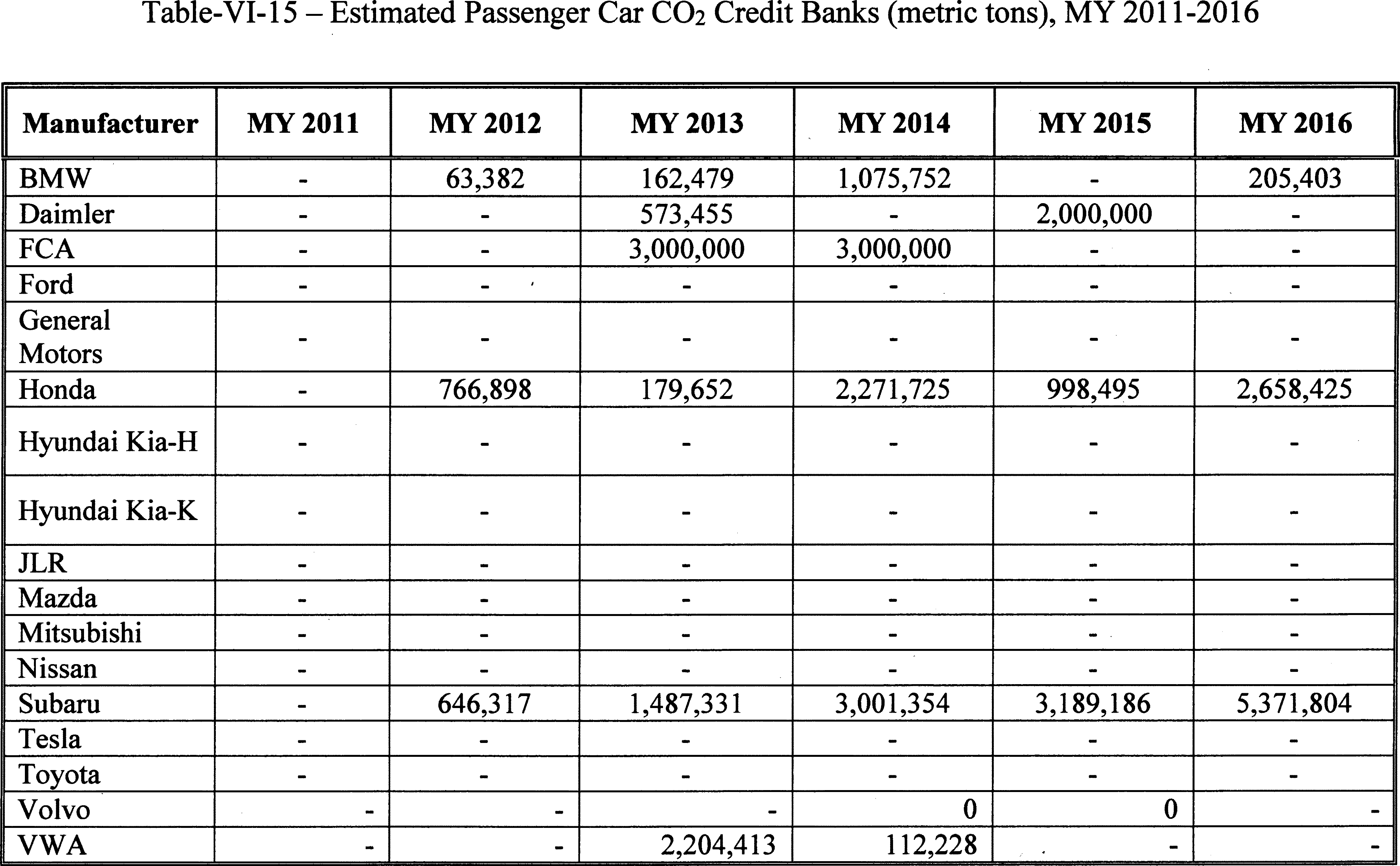

While the CAFE model does not simulate the ability to trade credits between manufacturers, it does simulate the strategic accumulation and application of compliance credits, as well as the ability to transfer credits between fleets to improve the compliance position of a less efficient fleet by leveraging credits earned by a more efficient fleet. The model prefers to hold on to earned compliance credits within a given fleet, carrying them forward into the future to offset potential future deficits. This assumption is consistent with observed strategic manufacturer behavior dating back to 2009.
From 2009 to present, no manufacturer has transferred CAFE credits into a fleet to offset a deficit in the same year in which they were earned. This has occurred with credits acquired from other manufacturers via trade but not with a manufacturer's own credits. Therefore, the current representation of credit transfers between fleets—where the model prefers to transfer expiring, or soon-to-be-expiring credits rather than newly earned credits—is both appropriate and consistent with observed industry behavior.
This may not be the case for CO2 standards, though it is difficult to be certain at this point. The CO2 program seeded the industry with a large quantity of early compliance credits (earned in MYs 2009-2011) [414] prior to the existence formal CO2 standards. Early credits from MYs 2010 and 2011, however, do not expire until 2021. Thus, for manufacturers looking to offset deficits, it is more sensible to exhaust credits that were generated during later model years (which are set to expire within the next five years), rather than relying on the initial bank of credits from MYs 2010 and 2011. The first model year for which earned credits outlive the initial bank is MY 2017, for which final manufacturer CO2 performance data (and hence, banked credits) has not yet been released. However, considering that under the CO2 program manufacturers simultaneously comply with passenger car and light truck fleets, to more accurately represent the CO2 credit system the CAFE model allows (and encourages) intra-year transfers between regulated fleets for the purpose of simulating compliance with the CO2 standards.
a) Off-Cycle and A/C Efficiency Adjustments to CAFE and Average CO2 Levels
In addition to more rigorous accounting of CAFE and CO2 credits, the model now also accounts for air conditioning efficiency and off-cycle adjustments. NHTSA's program considers those adjustments in a manufacturer's compliance calculation starting in MY 2017, and the NPRM version of the model used the adjustments claimed by each manufacturer in MY 2016 as the starting point for all future years. Because air conditioning efficiency and off-cycle adjustments are not credits in NHTSA's program, but rather adjustments to compliance fuel economy (much like the Flexible Fuel Vehicle adjustments due to phase out in MY 2019), they may be included under either a “standard setting” or “unconstrained” analysis perspective.
The manner in which the CAFE model treats the EPA and CAFE A/C efficiency and off-cycle credit programs is similar, but the model also accounts for A/C leakage (which is not part of NHTSA's program). When determining the compliance status of a manufacturer's fleet (in the case of EPA's program, PC and LT are the only fleet distinctions), the CAFE model weighs future compliance actions against the presence of existing (and expiring) CO2 credits resulting from over-compliance with earlier years' standards, A/C efficiency credits, A/C leakage credits, and off-cycle credits.
Another aspect of credit accounting, implemented in the NPRM version of the CAFE model, involved credits related to the application of off-cycle and A/C efficiency adjustments, which manufacturers earn by taking actions such as special window glazing or using reflective paints that provide fuel economy improvements in real-world operation but do not produce measurable improvements in fuel consumption on the 2-cycle test.
NHTSA's inclusion of off-cycle and A/C efficiency adjustments began in MY 2017, while EPA has collected several years' worth of submissions from manufacturers about off-cycle and A/C efficiency technology deployment. Currently, the level of deployment can vary considerably by manufacturer, with several claiming extensive Fuel Consumption Improvement Values (FCIV) for off-cycle and A/C efficiency technologies, and others almost none. The analysis of alternatives presented here (and in the NPRM) does not attempt to project how future off-cycle and A/C efficiency technology use will evolve or speculate about the potential proliferation of FCIV proposals submitted to the agencies. Rather, this analysis uses the off-cycle credits submitted by each manufacturer for MY 2017 compliance, and, with a few exceptions, carries these forward to future years. Several of the technologies described below are associated with A/C efficiency and off-cycle FCIVs. In particular, stop-start systems, integrated starter generators, and full hybrids are assumed to generate off-cycle adjustments when applied to vehicles to improve their fuel economy. Similarly, higher levels of aerodynamic improvements are assumed to include active grille shutters on the vehicle, which also qualify for off-cycle FCIVs.
The NPRM analysis assumed that any off-cycle FCIVs that are associated with actions outside of the technologies discussed in Section VI.C (either chosen from the pre-approved “pick list,” or granted in response to individual manufacturer petitions) remained at the levels claimed by manufacturers in MY 2017. Any additional A/C efficiency and off-cycle adjustments that accrued as the result of explicit technology application calculated dynamically in each model year for each alternative. The NPRM version of the CAFE model also represented manufacturers' credits for off-cycle improvements, A/C efficiency improvements, and A/C leakage reduction in terms of values applicable across all model years.
Recognizing that application of these improvements thus far varies considerably among manufacturers, such that some manufacturers have opportunities to earn significantly more of the corresponding adjustments over time, the agencies have expanded the CAFE model's representation of these credits to provide for year-by-year specification of the amounts of each type of adjustment for each manufacturer, denominated in grams CO2 per mile,[415] as summarized in the following table:


In addition to these refinements to the estimation of the quantities of adjustments earned over time by each manufacturer, the agencies revised the CAFE model to apply estimates of the corresponding costs. For today's analysis, the agencies applied estimates developed previously by EPA, adjusting these values to 2019 dollars. The following table summarizes inputs through model year 2030:

The model currently accounts for any off-cycle adjustments associated with technologies that are included in the set of fuel-saving technologies explicitly simulated as part of this proposal (for example, start-stop systems that reduce fuel consumption during idle or active grille shutters that improve aerodynamic drag at highway speeds) and accumulates these adjustments up to the 10 g/mi cap. As a practical matter, most of the adjustments for which manufacturers are claiming off-cycle FCIV exist outside of the technology tree, so the cap is rarely reached during compliance simulation. The agencies have considered the potential to model their application explicitly. However, doing so would require data regarding which vehicle models already possess these improvements as well as the cost and expected value of applying them to other models in the future. Such data is currently too limited to support explicit modeling of these technologies and adjustments.
b) Alternative Fuel Vehicles
When establishing maximum feasible fuel economy standards, NHTSA is prohibited from considering the availability of alternatively fueled vehicles,[417] and credit provisions related to AFVs that significantly increase their fuel economy for CAFE compliance purposes. Under the “standard setting” perspective, these technologies (pure battery electric vehicles and fuel cell vehicles) [418] are not available in the compliance simulation to improve fuel economy. Under the “unconstrained” perspective, such as is documented in the DEIS and FEIS, the CAFE model considers these technologies in the same manner as other available technologies, and may apply them if they represent cost-effective compliance pathways. However, under both perspectives, the analysis continues to include dedicated AFVs that already exist in the MY 2017 fleet (and their projected future volumes). Also, because the CAA provides no direction regarding consideration of alternative fuels, the final rule's analysis includes simulation of the potential that some manufacturers might introduce new AFVs in response to CO2 standards. To represent the compliance benefit from such a response fully, NHTSA modified the CAFE model to include the specific provisions related to AFVs under the CO2 standards. In particular, the CAFE model now carries a full representation of the production multipliers related to electric vehicles, fuel cell vehicles, plug-in hybrids, and CNG vehicles, all of which vary by year through MY 2021.
EPCA also provides that CAFE levels may, subject to limitations, be adjusted upward to reflect the sale of flexible fuel vehicles (FFVs). Although these adjustments end after model year 2020, the final rule's analysis, like the NPRM's, includes estimated potential use through MY 2019, as summarized below:

For its part, EPA has provided that manufacturers selling sufficient numbers of PHEVs, BEVs, and FCVs may, when calculating fleet average CO2 levels, “count” each unit of production as more than a single unit. The CAFE model accounts for these “multipliers.” As for the NPRM, the final rule's analysis applies the following multipliers:

For example, under EPA's current regulation, when calculating the average CO2 level achieved by its MY 2019 passenger car fleet, a manufacturer may treat each 1,000 BEVs as 2,000 BEVs. When calculating the average level required of this fleet, the manufacturer must use the actual production volume (in this example, 1,000 units). Similarly, the manufacturer must use the actual production volume when calculating compliance credit balances.
There were no natural gas vehicles in the baseline fleet, and the analysis did not apply natural gas technology due to cost effectiveness. The application of a 2.0 multiplier for natural gas vehicles for MYs 2022-2026 would have no impact on the analysis because given the state of natural gas vehicle refueling infrastructure, the cost to equip vehicles with natural gas tanks, the outlook for petroleum prices, and the outlook for battery prices, we have little basis to project more than an inconsequential response to this incentive in the foreseeable future.
For the final rule's analysis, the CAFE model can be exercised in a manner that simulates these current EPA requirements, or that simulates two alternative approaches. The first includes the above-mentioned multipliers in the calculation of average requirements, and the second also includes the multipliers in the calculation of credit balances. The central analysis reflects current regulations. The sensitivity analysis presented in the FRIA includes a case applying multipliers to the calculation of achieved and required average CO2 levels, and calculation of credit balances.
c) Civil Penalties
Throughout the history of the CAFE program, some manufacturers have consistently achieved fuel economy levels below applicable standards, electing instead to pay civil penalties as specified by EPCA. As in previous versions of the CAFE model, the current version allows the user to specify inputs identifying such manufacturers and to consider their compliance decisions as if they are willing to pay civil penalties for non-compliance with the CAFE program. As with the NPRM, the civil penalty rate in the current analysis is $5.50 per 1/10 of a mile per gallon, per vehicle manufactured for sale.
NHTSA notes that treating a manufacturer as if it is willing to pay civil penalties does not necessarily mean that it is expected to pay penalties in reality. Doing so merely implies that the manufacturer will only apply fuel economy technology up to a point, and then stop, regardless of whether or not its corporate average fuel economy is above its standard. In practice, the agencies expect that many of these manufacturers will continue to be active in the credit market, using trades with other manufacturers to transfer credits into specific fleets that are challenged in any given year, rather than paying penalties to resolve CAFE deficits. The CAFE model calculates the amount of penalties paid by each manufacturer, but it does not simulate trades between manufacturers. In practice, some (possibly most) of the total estimated penalties may be a transfer from one OEM to another.
Although EPCA, as amended in 2007 by the Energy Independence and Security Act (EISA), prescribes these specific civil penalty provisions for CAFE standards, the Clean Air Act (CAA) does not contain similar provisions. Rather, the CAA's provisions regarding noncompliance prohibit sale of a new motor vehicle that is not covered by an EPA certificate of conformity, and in order to receive such a certificate the new motor vehicle must meet EPA's Section 202 regulations, including applicable emissions standards. Therefore, inputs regarding civil penalties—including inputs regarding manufacturers' potential willingness to treat civil penalty payment as an economic choice—apply only to simulation of CAFE standards. On the other hand, some of the same manufacturers recently opting to pay civil penalties instead of complying with CAFE standards have also recently led adoption of lower-GWP refrigerants, and the “A/C leakage” credits count toward compliance only with CO2 standards, not CAFE standards. The model accounts for this difference between the programs.
When considering technology applications to improve fleet fuel economy, the model will add technology up to the point at which the effective cost of the technology (which includes technology cost, consumer fuel savings, consumer welfare changes, and the cost of penalties for non-compliance with the standard) is less costly than paying civil penalties or purchasing credits. Unlike previous versions of the model, the current implementation further acknowledges that some manufacturers experience transitions between product lines where they rely heavily on credits (either carried forward from earlier model years or acquired from other manufacturers) or simply pay penalties in one or more fleets for some number of years. The model now allows the user to specify, when appropriate for the regulatory program being simulated, on a year-by-year basis, whether each manufacturer should be considered as willing to pay penalties for non-compliance. This provides additional flexibility, particularly in the early years of the simulation. As discussed above, this assumption is best considered as a method to allow a manufacturer to under-comply with its standard in some model years—treating the civil penalty rate and payment option as a proxy for other actions it may take that are not represented in the CAFE model (e.g., purchasing credits from another manufacturer, carry-back from future model years, or negotiated settlements with NHTSA to resolve deficits).
For the NPRM, NHTSA relied on past compliance behavior and certified transactions in the credit market to designate some manufacturers as willing to pay CAFE penalties in some model years. The full set of NPRM assumptions regarding manufacturer behavior with respect to civil penalties is presented in Table VI-21, which shows all manufacturers were assumed to be willing to pay civil penalties prior to MY 2020. This was largely a reflection of either existing credit balances (which manufacturers will use to offset CAFE deficits until the credits reach their expiration dates) or inter-manufacturer trades assumed likely to happen in the near future, based on previous behavior. The manufacturers in the table whose names appear in bold all had at least one regulated fleet (of three) whose CAFE was below its standard in MY 2016. Because the NPRM analysis began with the MY 2016 fleet, and no technology could be added to vehicles that are already designed and built, all manufacturers could generate civil penalties in MY 2016. However, once a manufacturer is designated as unwilling to pay penalties, the CAFE model will attempt to add technology to the respective fleets to avoid shortfalls.

Several of the manufacturers in Table VI-21 that were presumed to be willing to pay civil penalties in the early years of the program have no history of paying civil penalties. However, several of those manufacturers have either bought or sold credits—or transferred credits from one fleet to another to offset a shortfall in the underperforming fleet. As the CAFE model does not simulate credit trades between manufacturers, providing this additional flexibility in the modeling avoids the outcome where the CAFE model applies more technology than needed in the context of the full set of compliance flexibilities at the industry level. By statute, NHTSA cannot consider credit flexibilities when setting standards, so most manufacturers (those without a history of civil penalty payment) are assumed to comply with their standards through fuel economy improvements for the model years being considered in this analysis. The notable exception to this assumption is Fiat Chrysler Automobiles (FCA), which could still satisfy the requirements of the program through a combination of credit application and civil penalties through MY 2025 before eventually complying exclusively through fuel economy improvements in MY 2026.
As mentioned above, the CAA does not provide civil penalty provisions similar to those provisions specified in EPCA/EISA, and the above-mentioned corresponding inputs apply only to simulation of compliance with CAFE standards.
Some stakeholders offering comments related to the analytical treatment of civil penalties indicated that NHTSA should tend toward assuming manufacturers will take advantage of this EPCA provision as an economically attractive alternative to compliance. Other commenters implied that NHTSA should tend toward not relying on compliance flexibilities in the analysis used to determine the maximum feasible stringency of CAFE standards. For example, New York University's Institute for Policy Integrity (IPI) offered the following comments:
NHTSA assumes that most manufacturers will be unwilling to pay penalties based in part on the fact that most manufacturers have not paid penalties in recent years. The Proposed Rule cites the statutory prohibition on NHTSA considering credit trading as a reason to assume manufacturers without a history of paying penalties will comply through technology alone, whatever the cost. But this is an arbitrary assumption and is in no way dictated by the statute. NHTSA knows as much, since elsewhere in the proposed rollback, the agency explains “EPCA is very clear as to which flexibilities are not to be considered” and NHTSA is allowed to consider off-cycle adjustments because they are not specifically mentioned. But considering penalties are not mentioned as off-limits for NHTSA in setting the standards either. Instead, the prohibition focuses on credit trading and transferring. The penalty safety valve has existed in EPCA for decades, and Congress clearly would have known how to add penalties to the list of trading and transferring. The fact that Congress did not bar NHTSA from considering penalties as a safety valve means that NHTSA must consider manufacturer's efficient use of penalties as a cost minimizing compliance option. Besides, NHTSA does consider penalties for some of the manufacturers making its statutory justification even less rational.[419]
On the other hand, in more general comments about NHTSA's analytical treatment of program flexibilities, FCA stated that “when flexibilities are considered while setting targets, they cease to be flexibilities and become simply additional technology mandates.” [420]
NHTSA agrees with IPI that EPCA does not expressly prohibit NHTSA, when conducting analysis supporting determinations of the maximum feasible stringency of future CAFE standards, from including manufacturers' potential tendency to pay civil penalties rather than complying with those standards. However, EPCA also does not require NHTSA to include this tendency in its analysis. NHTSA also notes, as does IPI, that EPCA does prohibit NHTSA from including credit trading, transferring, or the availability of credits in such analysis (although NHTSA interprets this prohibition to apply only to the model years for which standards are being set). This statutory difference is logical based on the way credits and penalties function differently under EPCA. Because credits help manufacturers achieve compliance with CAFE standards, absent the statutory prohibition, credits would be relevant to the feasibility of a standard.[421] Penalties, on the other hand, do not enable a manufacturer to comply with an applicable standard; penalties are for noncompliance.[422] When Congress added credit trading provisions to EPCA in 2007, NHTSA anticipated that competitive considerations would make manufacturers reluctant to engage in such trades. Since that time, manufacturers actually have demonstrated otherwise, although the reliance on trading—especially between specific pairs of OEMs—appears to vary widely. At this time, NHTSA considers it most likely that manufacturers will shift away from paying civil penalties and toward compliance credit trading. Consequently, for NHTSA to include civil penalty payment in its analysis would increasingly amount to using civil penalty payment as an analytical proxy for credit trading. Having further considered the question, NHTSA's current view is, therefore, that including civil penalty payment beyond MY 2020 would effectively subvert EPCA's prohibition against considering credit trading. Therefore, for today's announcement, NHTSA has modified its analysis to assume that BMW, Daimler, FCA, JLR, and Volvo would consider paying civil penalties through MY 2020, and that all manufacturers would apply as much technology as would be needed in order to avoid paying civil penalties after MY 2020.
3. Technology Effectiveness Values
The next input required to simulate manufacturers' decision-making processes for the year-by-year application of technologies to specific vehicles is estimates of how effective each technology would be at reducing fuel consumption. In the NPRM, the agencies used full-vehicle modeling and simulation to estimate the fuel economy improvements manufacturers could make to a fleet of vehicles, considering those vehicles' technical specifications and how combinations of technologies interact. Full-vehicle modeling and simulation uses computer software and physics-based models to predict how combinations of technologies perform as a full system under defined conditions.
A model is a mathematical representation of a system, and simulation is the behavior of that mathematical representation over time. In this analysis, the model is a mathematical representation of an entire vehicle,[423] including its individual components such as the engine and transmission, overall vehicle characteristics such as mass and aerodynamic drag, and the environmental conditions, such as ambient temperature and barometric pressure. The agencies simulated the model's behavior over test cycles, including the 2-cycle laboratory compliance tests (or 2-cycle tests),[424] to determine how the individual components interact. 2-cycle tests are test cycles that are used to measure fuel economy and emissions for CAFE and CO2 compliance, and therefore are the relevant test cycles for determining technology effectiveness when establishing standards. In the laboratory, 2-cycle testing involves sophisticated test and measurement equipment, carefully controlled environmental conditions, and precise procedures to provide the most repeatable results possible with human drivers. Measurements using these structured procedures serve as a yardstick for fuel economy and CO2 emissions.
Full-vehicle modeling and simulation was initially developed to avoid the costs of designing and testing prototype parts for every new type of technology. For example, if a truck manufacturer has a concept for a lightweight tailgate and wants to determine the fuel economy impact for the weight reduction, the manufacturer can use physics-based computer modeling to estimate the impact. The vehicle, modeled with the proposed change, can be simulated on a defined test route and under a defined test condition, such as city or highway driving in warm ambient temperature conditions, and compared against the baseline reference vehicle. Full-vehicle modeling and simulation allows the consideration and evaluation of different designs and concepts before building a single prototype. In addition, full vehicle modeling and simulation is beneficial when considering technologies that provide small incremental improvements. These improvements are difficult to measure in laboratory tests due to variations in how vehicles are driven over the test cycle by human drivers, variations in emissions measurement equipment, and variations in environmental conditions.[425]
Full-vehicle modeling and simulation requires detailed data describing the individual technologies and performance-related characteristics. Those specifications generally come from design specifications, laboratory measurements, and other subsystem simulations or modeling. One example of data used as an input to the full vehicle simulation are engine maps for each engine technology that define how much fuel is consumed by the engine technology across its operating range.
Using full-vehicle modeling and simulation to estimate technology efficiency improvements has two primary advantages over using single or limited point estimates. An analysis using single or limited point estimates may assume that, for example, one fuel economy improving technology with an effectiveness value of 5 percent by itself and another technology with an effectiveness value of 10 percent by itself, when applied together achieve an additive improvement of 15 percent. Single point estimates generally do not provide accurate effectiveness values because they do not capture complex relationships among technologies. Technology effectiveness often differs significantly depending on the vehicle type (e.g., sedan versus pickup truck) and how the technology interacts with other technologies on the vehicle, as different technologies may provide different incremental levels of fuel economy improvement if implemented alone or in tandem with other technologies. Any oversimplification of these complex interactions leads to less accurate and often overestimated effectiveness estimates.
In addition, because manufacturers often implement several fuel-saving technologies simultaneously when redesigning a vehicle, it is difficult to isolate the effect of individual technologies using laboratory measurement of production vehicles alone. Modeling and simulation offers the opportunity to isolate the effects of individual technologies by using a single or small number of baseline vehicle configurations and incrementally adding technologies to those baseline configurations. This provides a consistent reference point for the incremental effectiveness estimates for each technology and for combinations of technologies for each vehicle type. Vehicle modeling also reduces the potential for overcounting or undercounting technology effectiveness.
An important feature of this analysis is that the incremental effectiveness of each technology and combinations of technologies be accurate and relative to a consistent baseline vehicle. The absolute fuel economy values of the full vehicle simulations are used only to determine incremental effectiveness and are never used directly to assign an absolute fuel economy value to any vehicle model or configuration for the rulemaking analysis.
For this analysis, absolute fuel economy levels are based on the individual fuel economy values from CAFE compliance data for each vehicle in the baseline fleet. The incremental effectiveness from the full vehicle simulations performed in Autonomie, a physics-based full-vehicle modeling and simulation software developed and maintained by the U.S. Department of Energy's Argonne National Laboratory, are applied to baseline fuel economy to determine the absolute fuel economy of applying the first technology change. For subsequent technology changes, incremental effectiveness is applied to the absolute fuel economy level of the previous technology configuration.
For example, if a Ford F150 2-wheel drive crew cab and short bed in the baseline fleet has a fuel economy value of 30 mpg for CAFE compliance, 30 mpg will be considered the reference absolute fuel economy value. A similar full vehicle model in the Autonomie simulation may begin with an average fuel economy value of 32 mpg, and with incremental addition of a specific technology X its fuel economy improves to 35 mpg, a 9.3 percent improvement. In this example, the incremental fuel economy improvement (9.3 percent) from technology X would be applied to the F150's 30 mpg absolute value.
For this analysis, the agencies determined the incremental effectiveness of technologies as applied to the 2,952 unique vehicle models in the analysis fleet. Although, as mentioned above, full-vehicle modeling and simulation reduces the work and time required to assess the impact of moving a vehicle from one technology state to another, it would be impractical—if not impossible—to build a unique vehicle model for every individual vehicle in the analysis fleet. Therefore, as explained further below, vehicle models are built in a way that maintains similar attributes to the analysis fleet vehicles, which ensures key components are reasonably represented.
We received a wide array of comments regarding the full-vehicle modeling and simulation performed for the NPRM, but there was general agreement that full-vehicle modeling and simulation was the appropriate method to determine technology effectiveness.[426] Stakeholders commented on other areas, such as full vehicle simulation tools, inputs, and assumptions, and these comments will be discussed in the following sections. For this final rule, the agencies continued to use the same full-vehicle simulation approach to estimate technology effectiveness for technology adoption in the rulemaking timeframe. The next sections will discuss the details of the explicit input specifications and assumptions used for the final rule analysis.
a) Why This Rulemaking Used Autonomie Full-Vehicle Modeling and Simulation To Determine Technology Effectiveness
The NPRM and final rule analysis use effectiveness estimates for technologies developed using Autonomie, a physics-based full-vehicle modeling and simulation software developed and maintained by the U.S. Department of Energy's Argonne National Laboratory.[427] Autonomie was designed to serve as a single tool to meet requirements of automotive engineering throughout the vehicle development process, and has been under continuous improvement by Argonne for over 20 years. Autonomie is commercially available and widely used in the automotive industry by suppliers, automakers, and academic researchers (who publish findings in peer reviewed academic journals).[428] DOE and manufacturers have used Autonomie and its ability to simulate a large number of powertrain configurations, component technologies, and vehicle-level controls over numerous drive cycles to support studies on fuel efficiency, cost-benefit analysis, and carbon dioxide emissions,[429] and other topics.
Autonomie has also been used to provide the U.S. government with data to make decisions about future research, and is used by DOE for analysis supporting budget priorities and plans for programs managed by its Vehicle Technologies Office (VTO), and to support decision making among competing vehicle technology research and development projects.[430] In addition, Autonomie is the primary vehicle simulation tool used by DOE to support its U.S. DRIVE program, a government-industry partnership focused on advanced automotive and related energy infrastructure technology research and development.[431]
Autonomie is a MathWorks-based software environment and framework for automotive control-system design, simulation, and analysis.[432] It is designed for rapid and easy integration of models with varying levels of detail (low to high fidelity), abstraction (from subsystems to systems and entire architectures), and processes (e.g., calibration, validation). By building models automatically, Autonomie allows the quick simulation of many component technologies and powertrain configurations, and, in this case, to assess the energy consumption of advanced powertrain technologies. Autonomie simulates subsystems, systems, or entire vehicles; evaluates and analyzes fuel efficiency and performance; performs analyses and tests for virtual calibration, verification, and validation of hardware models and algorithms; supports system hardware and software requirements; links to optimization algorithms; and supplies libraries of models for propulsion architectures of conventional powertrains as well as hybrid and electric vehicles.
With hundreds of pre-defined powertrain configurations along with vehicle level control strategies developed from dynamometer test data, Autonomie is a highly capable tool for analyzing advantages and drawbacks of applying different technology options within each technology family, including conventional, parallel hybrid, power-split hybrid electric vehicles (HEVs), plug-in hybrid electric vehicles (PHEVs), battery electric vehicles (BEV) and fuel cell vehicles (FCVs). Autonomie also allows users to evaluate the effect of component sizing on fuel consumption for different powertrain technologies as well as to define component requirements (e.g., power, energy) to maximize fuel displacement for a specific application.[433] To evaluate properly any powertrain-configuration or component-sizing influence, vehicle-level control models are critical, especially for electric drive vehicles like hybrids and plug-in hybrids. Argonne has extensive expertise in developing vehicle-level control models based on different approaches, from global optimization to instantaneous optimization, rule-based optimization, and heuristic optimization.[434]
Autonomie has been developed to consider real-world vehicle metrics like performance, hardware limitations, utility, and drivability metrics (e.g., towing capability, shift busyness, frequency of engine on/off transitions), which are important to producing realistic estimates of fuel economy and CO2 emission rates. This increasing realism has, in turn, steadily increased confidence in the appropriateness of using Autonomie to make significant investment decisions. Autonomie has also been validated for a number of powertrain configurations and vehicle classes using Argonne's Advanced Mobility Technology Laboratory (AMTL) (formerly Advanced Powertrain Research Facility, or APRF) vehicle test data.[435]
Argonne has spent several years developing, applying, and expanding the means to use distributed computing to exercise its Autonomie full-vehicle simulation tool over the scale necessary for realistic analysis to provide data for CAFE and CO2 standards rulemaking. The NPRM and PRIA detailed how Argonne used Autonomie to estimate the fuel economy impacts for roughly a million combinations of technologies and vehicle types.[436 437] Argonne developed input parameters for Autonomie to represent every combination of vehicle, powertrain, and component technologies considered in this rulemaking. The sequential addition of more than 50 fuel economy-improving technologies to ten vehicle types generated more than 140,000 unique technology and vehicle combinations. Running the Autonomie powertrain sizing algorithms to determine the appropriate amount of engine downsizing needed to maintain overall vehicle performance when vehicle mass reduction is applied and for certain engine technology changes (discussed further, below) increased the total number of simulations to more than one million. The result of these simulations is a useful dataset identifying the impacts of combinations of vehicle technologies on energy consumption—a dataset that can be referenced as an input to the CAFE model for assessing regulatory compliance alternatives.
The following sections discuss the full-vehicle modeling and simulation inputs and data assumptions, and comments received on the NPRM analysis. The discussion is necessarily technical, but also important to understand the agencies' decisions to modify (or not) the Autonomie analysis for the final rule.
(1) Full-Vehicle Modeling, Simulation Inputs and Data Assumptions
The agencies provided extensive documentation that quantitatively and qualitatively described the over 50 technologies considered as inputs to the Autonomie modeling.[438 439] These inputs consisted of engine technologies, transmission technologies, powertrain electrification, light-weighting, aerodynamic improvements, and tire rolling resistance improvements.[440] The PRIA provided an overview of the sub-models for each technology, including the internal combustion engine model, automatic transmission model, and others.[441] The Argonne NPRM model documentation expanded on these sub-models in detail to show the interaction of each sub-model input and output.[442] For example, as shown in Figure VI-2, the input for Autonomie's driver model (i.e., the model used to approximate the driving behavior of a real driver) is vehicle speed, and outputs are accelerator pedal, brake pedal, and torque demand.

Effectiveness inputs for the NPRM and the final rule analysis were specifically developed to consider many real world and compliance test cycle constraints, to the extent a computer model could capture them. Examples include the advanced engine knock model discussed below, in addition to other constraints like allowing cylinder deactivation to occur in ways that would not negatively impact noise-vibration-harshness (NVH), and similarly optimizing the number of engine on/off events (e.g., from start/stop 12V micro hybrid systems) to balance between effectiveness and NVH.
One major input used in the effectiveness modeling that the agencies provided key specifications for in the PRIA are engine fuel maps that define how an engine equipped with specific technologies operates over a variety of engine load (torque) and engine speed conditions. The engine maps used as inputs to the Autonomie modeling portion of the analysis were developed by starting with a base map and then modifying that base map, incrementally, to model the addition of engine technologies. These engine maps, developed using the GT-Power modeling tool by IAV, were based off real-world engine designs. Simulated operation of these engines included the application of an IAV knock model, also developed from real-world engine data.[443 444] Using this process, which incorporated real-world data, ensured that real-world constraints were considered for each vehicle type. Although the same type of engine map is used for all technology classes, the effectiveness varies based on the characteristics of each vehicle type. For example, a compact car with a turbocharged engine will have different fuel economy and performance values than a pickup truck with the same engine technology type. The engine map specifications are discussed further in Section VI.C.1 of this preamble and Section VI of FRIA.
The agencies also provided key details about input assumptions for various vehicle specifications like transmission gear ratios, tire size, final drive ratios, and individual component weights.[445] Each of these assumptions, to some extent, varied between the ten technology classes to capture appropriately real-world vehicle specifications like wheel mass or fuel tank mass. These specific input assumptions were developed based on the latest test data and current market fleet information.[446] The agencies relied on default assumptions developed by the Autonomie team, based on test data and technical publication review, for other model inputs required by Autonomie, such as throttle time response and shifting strategies for different transmission technologies. The Autonomie modeling tool did not simulate vehicle attributes determined to have minimal impacts, like whether a vehicle had a sun roof or hood scoops, as those attributes would have trivial impact in the overall analysis.
Because the agencies model ten different vehicle types to represent the 2,952 vehicles in the baseline fleet, improper assumptions about an advanced technology could lead to errors in estimating effectiveness. Autonomie is a sophisticated full-vehicle modeling tool that requires extensive technology characteristics based on both physical and intangible data, like proprietary software. With a few technologies, the agencies did not have publicly available data, but had received confidential business information confirming such technologies potential availability in the market during the rulemaking time frame. For such technologies, including advanced cylinder deactivation, the agencies adopted a method in the CAFE model to represent the effectiveness of the technology, and did not explicitly simulate the technologies in the Autonomie model. For this limited set of technologies, the agencies determined that effectiveness could reasonably be represented as a fixed value.[447] Effectiveness values for technologies not explicitly simulated in Autonomie are discussed further in the individual technology sections of this preamble.
The agencies sought comments on all effectiveness inputs and input assumptions, including the specific data used to characterize the technologies, such as data to build the technology input, data representing operating range of technologies, and data for variation among technology inputs. The agencies also sought comment on the effectiveness values used for technologies not explicitly defined in Autonomie.
Meszler Engineering Services, commenting on behalf of the Natural Resources Defense Council, and ICCT questioned the accuracy of the effectiveness estimates in the Argonne database, and as an example Meszler analyzed the fuel economy impacts of a 10-speed automatic transmission relative to a baseline 8-speed automatic transmission, concluding that the widely ranging effectiveness estimates were unexpected. ICCT questioned the accuracy of the IAV engine maps that serve as an input to the Autonomie effectiveness modeling, and asked whether those could “reasonably stand as a foundation for automotive developments and technology combinations” discussed elsewhere in their comments. ICCT also questioned whether Autonomie realistically and validly modeled synergies between technologies, using the effectiveness values from CEGR and transmissions as an example. Meszler stated that the agencies have an obligation to validate the Autonomie estimates before using them to support the NPRM or any other rulemaking. The agencies also received comments on the specific effectiveness estimates generated by Autonomie; however, those comments will be discussed in each individual technology section, below.
Despite these criticisms, Meszler stated that the critiques of the Autonomie technology database were not meant to imply that the Autonomie vehicle simulation model used to develop the database was fundamentally flawed, or that the model could not be used to derive accurate fuel economy impact estimates. Meszler noted that, as with any model, estimates derived with Autonomie are only valid for a given set of modeling parameters and if those parameters are well defined, the estimates should be accurate and reliable. Conversely, if those parameters are not well defined, the estimates would be inaccurate and unreliable. Meszler stated that the agencies must make the full set of modeling assumptions used for the Autonomie database available for review and comment.
We agree with Meszler that, in general, when inputs to a model are inaccurate, output effectiveness results may be too high or too low. The technology effectiveness estimates from modeling results often vary with the type of vehicle and the other technologies that are on that vehicle.[448] The Autonomie output database consists of permutations of over 50 technologies for each of the ten technology classes simulated by the CAFE model. A wide range of effectiveness is expected when going from a baseline technology to an advanced technology across different technology classes because there are significant differences in how much power is required from the powertrain during 2-cycle testing across the ten vehicle types. This impacts powertrain operating conditions (e.g., engine speed and load) during 2-cycle testing. Fuel economy improving technologies have different effectiveness at each of those operating conditions so vehicles that have higher average power demands will have different effectiveness than vehicles with lower average power demands. Further, the differences in effectiveness at higher power and lower power vary by technology so the overall relationship is complex. Large-scale full-vehicle modeling and simulation account for these interactions and complexities.
Before conducting any full-vehicle modeling and simulation, the agencies spent a considerable amount of time and effort developing the specific inputs used for the Autonomie analysis. The agencies believe that these technology inputs provide reasonable estimates for the light-duty vehicle technologies the agencies expect to be available in the market in the rulemaking timeframe. As discussed earlier, these inputs vary in effectiveness due to how different vehicles, like compact cars and pickup trucks, operate on the 2-cycle test and in the real world. Some technologies, such as 10-speed automatic transmissions (AT10) relative to 8-speed automatic transmissions (AT8), can and should have different effectiveness results in the analysis between two different technology classes.[449] These unique synergistic effects can only be taken into account through conducting full-vehicle modeling and simulation, which the agencies did here.
With regards to Meszler's comment that the agencies have an obligation to validate the Autonomie estimates before using them to support the NPRM or any other rulemaking, the agencies would like to point Meszler to the description of the Argonne Autonomie team's robust process for vehicle model validation that was contained in the PRIA.[450] To summarize, the NPRM and final rule analysis leveraged extensive vehicle test data collected by Argonne National Laboratory.[451] Over the past 20 years, the Argonne team has developed specific instrumentation lists and test procedures for collecting sufficient information to develop and validate full vehicle models. In addition, the agencies described the Argonne team's efforts to validate specific component models as well, such as the advanced automatic transmission and dual clutch transmission models.[452]
The agencies also described the process for validating inputs used to develop the IAV engine maps,[453 454] another input to the Autonomie simulations. As discussed in the PRIA, IAV's engine model development relied on a collection of sub-models that controlled independent combustion characteristics such as heat release, combustion knock, friction, heat flow, and other combustion optimization tools. These sub-models and other computational fluid dynamics models were utilized to convert test data for use in the IAV engine map development. Specific combustion parameters, like from test data for the coefficient of variation for the indicated mean effective pressure (COV of IMEP), which is a common variable for combustion stability in a spark ignited engine, was used to assure final engine models were reasonable. The assumptions and inputs used in the modeling and validation of engine model results leveraged IAV's global engine database, which included benchmarking data, engine test data, single cylinder test data and prior modeling studies, and also technical publications and information presented at conferences. The agencies referenced in the PRIA that engine maps were validated with engine dynamometer test data to the maximum extent possible.[455] Because the NPRM and the final rule analysis considered some technologies not yet in production, the agencies relied on technical publications and engine modeling by IAV to develop and corroborate inputs and input assumptions where engine dynamometer test data was not available.
In addition, as described earlier in this section, the full set of NPRM modeling assumptions used for the Autonomie database were available for review and comment in the docket for this rulemaking.[456] The full set of modeling assumptions used for the final rule are also available in the docket.[457]
Both ICCT and Meszler also commented on the availability of technologies within the Autonomie database, with Meszler stating that with limited exceptions, technologies were not included in the NPRM CAFE model if they were not included in the simulation modeling that underlay the Argonne database, and accordingly if a combination of technologies was not modeled during the development of the Argonne database, that package (or combination) of technologies was not available for adoption in the CAFE model. Meszler stated that these constraints limited the slate of technologies available to respond to fuel economy standards, and independently expanding the model to include additional technologies or technology combinations is not trivial.
ICCT gave specific examples of key efficiency technologies that it stated Autonomie did not include, like advanced DEAC, VCR, Miller Cycle, e-boost, and HCCI. ICCT argued that this was especially problematic as the agencies appeared to have available engine maps from IAV on advanced DEAC, VCR, Miller Cycle, E-boost (and from advanced DEAC, VCR, Miller Cycle, E-boost, HCCI from EPA) that Argonne or the agencies have been unable to or opted not to include in their modeling. ICCT stated that the agencies must disclose how Autonomie had been updated to incorporate “cutting edge” 2020-2025 automotive technologies to ensure they reflect available improvements.[458]
The agencies have updated the final rule analysis to include additional technologies. In the NPRM, the agencies presented the engine maps for all of the technologies that ICCT listed, except HCCI, and sought comment on the engine maps, technical assumptions and the potential use of the technologies for the final rule analysis. Based on the available technical information and the ICCT and Meszler comments, for the final rule analysis, VCR, Miller Cycle (VTG), and e-boost (VTGe with 48V BISG) technologies have been added and included in the Autonomie modeling and simulations, and advanced DEAC technology has been added using fixed point effectiveness estimates in the CAFE model analysis. The agencies disagree with ICCT's assessment of HCCI and do not believe it will be available for wide-scale application in the rulemaking timeframe, and therefore have not included it as a technology. HCCI technology has been in the research phase for several decades, and the only production applications to date use a highly-limited version that restricts HCCI combustion to a very narrow range of engine operating conditions.[459 460 461] Additional discussion of how Autonomie-modeled and non-modeled technologies are incorporated into the CAFE Model is located in Section VI.B.3.c), below.
ICCT and Meszler also commented that the agencies overly limited the availability of several technologies in the NPRM analysis. In response, the agencies reconsidered the restrictions that were applied in the NPRM analysis, and agree with the commenters for several technologies and technology classes. Many technologies identified by the commenters are now in production for the MY2017 as well as MY2018 and MY2019. The agencies also think that the baseline fleet compliance data reflects adoption of many of these technologies. For the final rule analysis, the agencies have expanded the availability of several technologies. In the CAFE model, the agencies are now allowing parallel hybrids (SHEVP2) to be adopted with high compression Atkinson mode engines (HCR0 and HCR1). In addition, as mentioned above, the Autonomie full-vehicle modeling included Variable Compression Ratio engine (VCR), Miller Cycle Engine (VTG), E-boost (VTGe) technologies, and cylinder deactivation technologies (DEAC) to be applied to turbocharged engines (TURBO1). As these changes relate to the technology effectiveness modeling, the CAFE model analysis now includes effectiveness estimates based on full vehicle simulations for all of these technology combinations.
We disagree with comments stating the agencies should allow every technology to be available to every vehicle class.[462] Discussed earlier in this section, Autonomie models key aspects of vehicle operation that are most relevant to assessing fuel economy, vehicle performance and certain aspects of drivability (like EPA 2-cycle tests, EPA US06 cycle tests, gradability, low speed acceleration time from 0-to-60 mph, passing acceleration time from 50 to 80 mph, and number of transmission shifts). However, there are other critical aspects of vehicle functionality and operation that the agencies considered beyond those criteria, that cannot necessarily be reflected in the Autonomie modeling. For example, a pickup truck can be modeled with a continuously variable transmission (CVT) and show improvements on the 2-cycle tests. However, pickup trucks are designed to provide high load towing utility.[463] CVTs lack the torque levels needed to provide that towing utility, and would fail mechanically if subject to high load towing.[464] The agencies provided discussions of some of these technical considerations in the PRIA, and explained why the agencies had limited technologies for certain vehicle classes, such as limiting CVTs on pickups as in the example above. These and other limitations are discussed further in the individual technology sections.
The agencies also received a variety of comments that conflated aspects of the Autonomie models with technology inputs and input assumptions. For example, commenters expressed concern about the transmission gear set and final drive values used for the NPRM analysis, or more specifically, that the gear ratios were held constant across applications.[465] In this case, both the inputs (gear set and final drive ratio) and input assumption (ratios held constant) were discussed by the commenters. Because these comments are actually about technology inputs to the Autonomie model, for these and similar cases, the agencies are addressing the comments in the individual technology sections which discuss the technology inputs and input assumptions that impact the effectiveness values for those technologies.
For the NPRM analysis, the agencies prioritized using inputs that were based on data for identifiable technology configurations and that reflected practical real world constraints. The agencies provided detailed information on the NPRM analysis inputs and input assumptions in the NPRM Preamble, PRIA and Argonne model documentation for engine technologies, transmission technologies, powertrain electrification, light-weighting, aerodynamic improvements, tire rolling resistance improvements, and other vehicle technologies. Comments and the agencies' assessment of comments for each technology are discussed in the individual technology sections below. Through careful consideration of the comments, the agencies have updated analytical inputs associated with several technologies, and as discussed above, have included several advanced technologies for which technical information was included in the NPRM. However, for most technologies, the agencies have determined that the technology inputs and input assumptions that were used in the NPRM analysis remain reasonable and the best available for the final rule analysis.
(2) How The Agencies Defined Different Vehicle Types in Autonomie
As described in the NPRM, Argonne produced full-vehicle models and ran simulations for many combinations of technologies, on many types of vehicles, but it did not simulate literally every single vehicle model/configuration in the analysis fleet because it would be impractical to assemble the requisite detailed information—much of which would likely only be provided on a confidential basis—specific to each vehicle model/configuration and because the scale of the simulation effort would correspondingly increase by orders of magnitude. Instead, Argonne simulated 10 different vehicle types, corresponding to the five “technology classes” generally used in CAFE analysis over the past several rulemakings, each with two performance levels and corresponding vehicle technical specifications (e.g., small car, small performance car, pickup truck, performance pickup truck, etc.).
Technology classes are a means of specifying common technology input assumptions for vehicles that share similar characteristics. Because each vehicle technology class has unique characteristics, the effectiveness of technologies and combinations of technologies is different for each technology class. Conducting Autonomie simulations uniquely for each technology class provides a specific set of simulations and effectiveness data for each technology class. Like the Draft TAR analysis, there are separate technology classes for compact cars, midsize cars, small SUVs, large SUVs, and pickup trucks. However, new for the NPRM analysis and carried into this final rule analysis, each of those vehicle types has been split into “low” (or “standard”) performance and a “high” performance versions, which represent two classes with similar body styles but different levels of performance attributes (for a total of 10 technology classes). The separate technology classes for high performance and low performance vehicles better account for performance diversity across the fleet.
NHTSA directed Argonne to develop a vehicle assumptions database to capture vehicle attributes that would comprise the full vehicle models. For each vehicle technology class, representative vehicle attributes and characteristics were identified from publicly available information and automotive benchmarking databases like A2Mac1,[466] Argonne's Downloadable Dynamometer Database (D[3] ),[467] and EPA compliance and fuel economy data,[468] EPA's guidance on the cold start penalty on 2-cycle tests.[469] The resulting vehicle assumptions database consists of over 100 different attributes like vehicle frontal area, drag coefficient, fuel tank weight, transmission housing weight, transmission clutch weight, hybrid vehicle component weights, and weights for components that comprise engines and electric machines, tire rolling resistance, transmission gear ratios and final drive ratio. Each of the 10 different vehicle types was assigned a set of these baseline attributes and characteristics, to which combinations of fuel-saving technologies were added as inputs for the Autonomie simulations. For example, the characteristics of the MY 2016 Honda Fit were considered along with a wide range of other compact cars to identify representative characteristics for the Autonomie simulations for the base compact car technology class. The simulations determined the fuel economy achieved when applying each combination of technologies to that vehicle type, given its baseline characteristics.
For each vehicle technology class and for each vehicle attribute, Argonne estimated the attribute value using statistical distribution analysis of publicly available data and data obtained from the A2Mac1 benchmarking database.[470] Some vehicle attributes were also based on test data and vehicle benchmarking, like the cold-start penalty for the FTP test cycle and vehicle electrical accessories load. The analysis of vehicle attributes used in the NPRM was discussed in the Argonne model documentation,[471] and values for each vehicle technology class were provided with the NPRM for public review.[472]
The agencies did not believe it was appropriate to assign one single engine mass for each vehicle technology class in the NPRM analysis. To account for the difference in weight for different engine types, Argonne performed a regression analysis of engine peak power versus weight, based on attribute data taken from the A2Mac1 benchmarking database. For example, to account for weight of different engine sizes like 4-cylinder versus 8-cylinder, Argonne developed a relationship curve between peak power and engine weight based on the A2Mac1 benchmarking data. For the NPRM analysis, this relationship was used to estimate mass for all engine types regardless of technology type (e.g., variable valve lift and direct injection). Secondary weight reduction associated with changes in engine technology was applied by using this linear relationship between engine power and engine weight from the A2Mac1 benchmarking database. When a vehicle in the analysis fleet with an 8-cylinder engine adopted a more fuel efficient 6-cylinder engine, the total vehicle weight would reflect the updated engine weight with two less cylinders based on the peak power versus engine weight relationship. The impact of engine mass reduction on effectiveness is accounted for directly in the Autonomie simulation data through the application of the above relationship. Engine mass reduction through downsizing is, therefore, appropriately not included as part of vehicle mass reduction technology that is discussed in Section VI.C.4 because doing so would result in double counting the impacts. As discussed further below, for the final rule the agencies improved upon the precision of engine weights by creating two curves to separately represent naturally aspirated engine designs and turbocharged engine designs.
In addition, certain attributes were held at constant levels within each technology class to maintain vehicle functionality, performance and utility including noise, vibration, and harshness (NVH), safety, performance and other utilities important for customer satisfaction. For example, in addition to the vehicle performance constraints discussed in Section VI.B.3.a)(6), the analysis does not allow the frontal area of the vehicle to change, in order to maintain utility like ground clearance, head-room space, and cargo space, and a cold-start penalty is used to account for fuel economy degradation for heater performance and emissions system catalyst light-off.[473] This allows us to capture the discrete improvement in technology effectiveness while maintaining vehicle attributes that are important vehicle utility, consumer acceptance and compliance with criteria emission standards, and considering these constraints similar to how manufacturers do in the real world.
The agencies sought comment on the analytical approach used to determine vehicle attributes and characteristics for the Autonomie modeling. In response, the agencies received a wide variety of comments on vehicle attributes ranging from discussions of performance increase from technology adoption (e.g., if a vehicle adopting an electrified powertrain improved its time to accelerate from 0-60 mph), to comments on vehicle attributes not modeled in Autonomie, like heated seats and cargo space.
Toyota and the Alliance commented that the inclusion of performance vehicle classes addressed the market reality that some consumers will purchase vehicles for their performance attributes and will accept the corresponding reduction in fuel economy. Furthermore, Toyota commented that some gain in performance is more realistic, and that “dedicating all powertrain improvements to fuel efficiency is inconsistent with market reality.” Toyota “supports the agencies' inclusion of performance classes in compliance modeling where a subset of certain models is defined to have higher performance and a commensurate reduction in fuel efficiency.” [474] Also, in support of the addition of performance vehicle classes, the Alliance commented that “vehicle categories have been increased to 10 to better recognize the range of 0-60 performance characteristics within each of the 5 previous categories, in recognition of the fact that many vehicles in the baseline fleet significantly exceeded the previously assumed 0-60 performance metrics. This provides better resolution of the baseline fleet and more accurate estimates of the benefits of technology.” [475]
UCS commented that the CAFE model incorporates technology improvements to each vehicle by applying the effectiveness improvement of the average vehicle in the technology class, leading to discrete “stepped” effectiveness levels for technologies across the different vehicle types. UCS stated that in contrast, the OMEGA model takes into account a vehicle's performance characteristics through response-surface modeling based on relative deviation from the class average modeled in ALPHA.[476]
Although differences between the ALPHA and Autonomie models are discussed in more detail below, for the NPRM vehicle simulation analysis the agencies expanded the number of vehicle classes from the five classes used in the Draft TAR to ten classes, to represent better the diversity of vehicle characteristics across the fleet. Each of these ten vehicle technology classes are empirically built from benchmarking data and other information from various sources, amounting to hundreds of vehicle characteristics data points to develop each vehicle class. The agencies expand on these vehicle classes and characteristics in Section VI.B.3.(a)(2) Vehicle Types in Autonomie and Section VI.B.3.(a)(3) How Vehicle Models are Built in Autonomie and Optimized for Simulation. The agencies believe that the real-world data used to define vehicle characteristics for each of the ten vehicle classes, in addition to the ten vehicle technology classes themselves, ensures the analysis reasonably accounts for the diversity in vehicle characteristics across the fleet.
The agencies believe that UCS's characterization of how technology improvements are applied in the analysis is a misleading oversimplification. While the analysis approach in the final rule uses a representative effectiveness value, the value is not linked solely to the vehicle technology class, as the UCS implies. The entire technology combination, or technology key, which includes the vehicle technology class, is used to determine the value for the platform being considered. Within each vehicle class, the interactions between the added technology and the full vehicle system (including other technologies and substantial road load characteristics) are considered in the effectiveness values calculated for each technology during compliance modeling. As discussed under each of the technology pathways sections, the effectiveness for most technologies is reported as a range rather than a single value. The range exists because the effectiveness for each technology is adjusted based on the technologies it is coupled with and the major road load characteristics of the full vehicle system. This approach, in combination with using the baseline vehicle's initial performance values as a starting point for performance improvement, results in a widely variable level of improvement for the system, dependent on individual vehicle platform characteristics. As a result, the application of a response-surface approach would likely result in minimal improvement in accuracy for the Autonomie and CAFE model analysis approach.
For the final rule analysis, the agencies used the same process to obtain the vehicle attributes and characteristics for the vehicle technology classes. Data was acquired from publicly available sources, Argonne D3, EPA compliance and fuel economy data, and A2mac1 benchmarking data. Accordingly, the attributes and characteristics of the modeled vehicles reflect actual vehicles that meet customer expectations and automakers' capabilities to manufacture the vehicles. In addition, for the final rule, the agencies improved the NPRM analysis by updating some of the attribute values to account for changes in the fleet. For example, the agencies have updated vehicle electrical accessory load on the test cycle to reflect higher electrical loads associated with contemporary vehicle features.
(3) How This Rulemaking Builds Vehicle Models for Autonomie and Optimize Them for Simulation
Before any simulation is initiated in Autonomie, Argonne must “build” a vehicle by assigning reference technologies and initial attributes to the components of the vehicle model representing each technology class.[477] The reference technologies are baseline technologies that represent the first step on each technology pathway used in the analysis. For example, a compact car is built by assigning it a baseline engine, a baseline 6-speed automatic transmission (AT6), a baseline level of aerodynamic improvement (AERO0), a baseline level of rolling resistance improvement (ROLL0), a baseline level of mass reduction technology (MR0), and corresponding attributes from the Argonne vehicle assumptions database like individual component weights.[478] A baseline vehicle will have a unique starting point for the simulation and a unique set of assigned inputs and attributes, based on its technology class.
The next step in the process is to run a powertrain sizing algorithm that ensures the built vehicle meets or exceeds defined performance metrics, including low-speed acceleration (i.e., time required to accelerate from 0-60 mph), high-speed passing acceleration (time required to accelerate from 50-80 mph), gradeability (e.g. the ability of the vehicle to maintain constant 65 miles per hour speed on a six percent upgrade), and towing capacity. Together, these performance criteria are widely used by industry as metrics to quantify vehicle performance attributes that consumers observe and that are important for vehicle utility and customer satisfaction.
In the compact car example used above, the agencies assigned an initial specific engine design and engine power, transmission, AERO, ROLL, and MR technologies, and other attributes like vehicle weight. If the built vehicle does not meet all the performance criteria in the first iteration, then the engine power is increased to meet the performance requirement. This increase in power is from higher engine displacement, which could involve an increase in number of cylinders, leading to an increase in the engine weight. The iterative process continues to check whether the compact car with updated engine power, and corresponding updated engine weight, meets its defined performance metrics. The loop stops once all the metrics are met, and at this point, a compact car technology class vehicle model becomes ready for simulation. For further discussion of the vehicle performance metrics, see Section VI.B.3.(a).
Autonomie then adopts a single fuel saving technology to the baseline vehicle model, keeping everything else the same except for that one technology and the attributes associated with it. For example, the model would apply an 8-speed automatic transmission in place of the baseline 6-speed automatic transmission, which would lead to either an increase or decrease in the total weight of the vehicle based on the technology class assumptions. At this point, Autonomie confirms whether performance metrics are met for this new vehicle model through the previously discussed sizing algorithm. Once a technology has been assigned to the vehicle model and the resulting vehicle meets its performance metrics, those vehicle models will be used as inputs to the full vehicle simulations. So, in the example of the 6-speed to 8-speed automatic transmission technology update, the agencies now have the initial ten vehicle models (one for each technology class), plus the ten new vehicle models with the updated 8-speed automatic transmission, which adds up to 20 different vehicle models for simulation. This permutation process is conducted for each of the over 50 technologies considered, and for all ten technology classes, which results in more than one million optimized vehicle models.
Figure VI-3 shows the process for building vehicles in Autonomie for simulation.

Some of the technologies require extra steps for optimization before the vehicle models are built for simulation; for example, the sizing and optimization process is more complex for the electrified vehicles (i.e., HEVs, PHEVs) compared to vehicles with internal combustion engines, as discussed further, below. Throughout the vehicle building process, the following items are considered for optimization:
- Vehicle weight is decreased or increased in response to switching from one type of technology to another for the technologies for which the agencies consider weight, such as different engine and transmission types;
- Vehicle performance is decreased or increased in response to the addition of mass reduction technologies when switching from one vehicle model to another vehicle model for the same engine;
- Vehicle performance is decreased or increased in response to the addition of a new technology when switching from one vehicle model to another vehicle model for the same hybrid electric machine; and
- Electric vehicle battery size is decreased or increased in response to the addition of mass, aero and/or tire rolling resistance technologies when switching from one vehicle model to another vehicle model.
Every time a vehicle adopts a new technology, the vehicle weight is updated to reflect the new component weight. For some technologies, the direct weight change is easy to assess. For example, in the NPRM the agencies designated weights for transmissions so, when a vehicle is updated to a higher geared transmission, the weight of the original transmission is replaced with the corresponding transmission weight (e.g., the weight of a vehicle moving from a 5-speed automatic transmission to an 8-speed automatic transmission will be updated based on the 8-speed transmission weight).
For other technologies, like engine technologies, assessing the updated vehicle weight is much more complex. Discussed earlier, modeling a change in engine technology involves both the new technology adoption and a change in power (because the reduction in vehicle weight leads to lower engine loads, and a resized engine). When a new engine technology is adopted on a vehicle the agencies account for the associated weight change to the vehicle based on the earlier discussed regression analysis of weight versus power. For the NPRM engine weight regression analysis, the agencies considered 19 different engine technologies that consisted of unique components to achieve fuel economy improvements. This regression analysis is technology agnostic by taking the approach of using engine peak power versus engine weight because it removed biases to any specific engine technology in the analysis. Although the agencies do not estimate the specific weight for each individual engine technology, such as VVT and SGDI, this process provides a reasonable estimate of the weight differences among engine technologies.
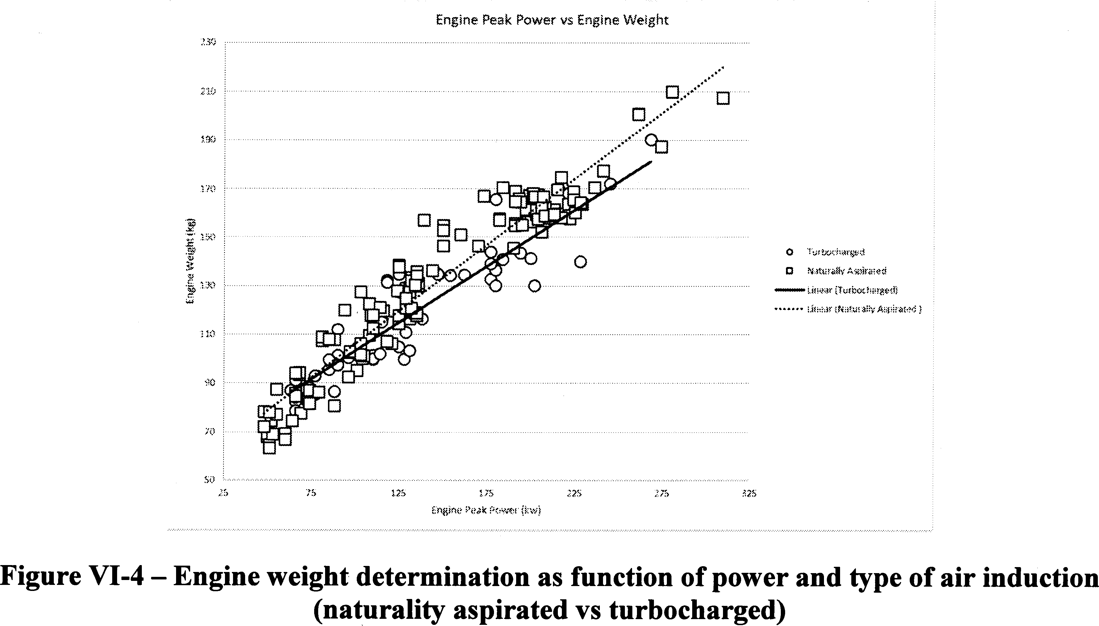
For the final rule analysis, the agencies used the same process to assign initial weights to the original 19 engines, plus the added engines. However, the agencies improved upon precision of the weights by creating two separate curves separately to represent naturally aspirated engine designs and turbocharged engine designs.[479] This update resulted in two benefits. First, small naturally aspirated 4-cylinder engines that adopted turbocharging technology reflected the increased weight of associated components like ducting, clamps, the turbocharger itself, a charged air cooler, wiring, fasteners, and a modified exhaust manifold. Second, larger cylinder count engines like naturally aspirated 8-cylinder and 6-cylinder engines that adopted turbocharging and downsized technologies would have lower weight due to having fewer engine cylinders. For example, a naturally aspirated 8-cylinder engine that adopts turbocharging technology when downsized to a 6-cylinder turbocharged engine appropriately reflects the added weight of turbocharging components, and the lower weight of fewer cylinders.
As with conventional vehicle models, electrified vehicle models were built from the ground up. For the NPRM analysis, Argonne used data from the A2mac1 database and vehicle test data to define different attributes like weights and power. Argonne used one electric motor specific power for each type of hybrid and electric vehicle.[480] For MY2017, the U.S. market has an expanded number of available hybrid and electric vehicle models. To capture appropriately the improvements for electrified vehicles for the final rule analysis, the agencies applied the same regression analysis process that considers electric motor weight versus electric motor power for vehicle models that have adopted electric motors. Benchmarking data for hybrid and electric vehicles from the A2Mac1 database was analyzed to develop a regression curve of electric motor peak power versus electric motor weight.[481]
(4) How Autonomie Sizes Powertrains for Full Vehicle Simulation
The agencies maintain performance neutrality of the full vehicle simulation analysis by resizing engines, electric machines, and hybrid electric vehicle battery packs at specific incremental technology steps. To address product complexity and economies of scale, engine resizing is limited to specific incremental technology changes that would typically be associated with a major vehicle or engine redesign.[482] Manufacturers have repeatedly told the agencies that the high costs for redesign and the increased manufacturing complexity that would result from resizing engines for small technology changes preclude them from doing so. It would be unreasonable and unaffordable to resize powertrains for every unique combination of technologies, and exceedingly so for every unique combination of technologies across every vehicle model due to the extreme manufacturing complexity that would be required to do so. The agencies reiterated in the NPRM that the analysis should not include engine resizing with the application of every technology or for combinations of technologies that drive small performance changes so that the analysis better reflects what is feasible for manufacturers.[483]
When a powertrain does need to be resized, Autonomie attempts to mimic manufacturers' development approaches to the extent possible. Discussed earlier, the Autonomie vehicle building process is initiated by building a baseline vehicle model with a baseline engine, transmission, and other baseline vehicle technologies. This baseline vehicle model (for each technology class) is sized to meet a specific set of performance criteria, including acceleration and gradeability.
The modeling also accounts for the industry practice of platform, engine, and transmission sharing to manage component complexity and the associated costs.[484] At a vehicle refresh cycle, a vehicle may inherit an already resized powertrain from another vehicle within the same engine-sharing platform that adopted the powertrain in an earlier model year. In the Autonomie modeling, when a new vehicle adopts fuel saving technologies that are inherited, the engine is not resized (the properties from the baseline reference vehicle are used directly and unchanged) and there may be a small change in vehicle performance. For example, in Figure VI-3, Vehicle 2 inherits Eng01 from Vehicle 1 while updating the transmission. Inheritance of the engine with new transmission may change performance. This example illustrates how manufacturers generally manage manufacturing complexity for engines, transmissions, and electrification technologies.
Autonomie implements different powertrain sizing algorithms depending on the type of powertrain being considered because different types of powertrains contain different components that must be optimized.[485] For example, the conventional powertrain resizing considers the reference power of the conventional engine (e.g., Eng01, a basic VVT engine, is rated at 108 kilowatts and this is the starting reference power for all technology classes) against the power-split hybrid (SHEVPS) resizing algorithm that must separately optimize engine power, battery size (energy and power), and electric motor power. An engine's reference power rating can either increase or decrease depending on the architecture, vehicle technology class, and whether it includes other advanced technologies.
Performance requirements also differ depending on the type of powertrain because vehicles with different powertrain types may need to meet different criteria. For example, a plug-in hybrid electric vehicle (PHEV) powertrain that is capable of traveling a certain number of miles on its battery energy alone (referred to as all-electric range, or AER, or as performing in electric-only mode) is also sized to ensure that it can meet the performance requirements of a US06 cycle in electric-only mode.
The powertrain sizing algorithm is an iterative process that attempts to optimize individual powertrain components at each step. For example, the sizing algorithm for conventional powertrains estimates required power to meet gradeability and acceleration performance and compares it to the reference engine power for the technology class. If the power required to meet gradeability and acceleration performance exceeds the reference engine power, the engine power is updated to the new value. Similarly, if the reference engine power exceeds the gradeability and acceleration performance power, it will be decreased to the lower power rating. As the change in power requires a change design of the engine, like increasing displacement (e.g., going from a 5.2-liter to 5.6-liter engine, or vice versa) or increasing cylinder count (e.g., going from an I4 to a V6 or vice versa), the engine weight will also change. The new engine power is used to update the weight of the engine.
Next, the conventional powertrain sizing algorithm enters an acceleration algorithm loop to verify low-speed acceleration performance (time it takes to go from 0 mph to 60 mph). In this step, Autonomie adjusts engine power to maintain a performance attribute for the given technology class and updates engine weight accordingly. Once the performance criteria are met, Autonomie ends the low-speed acceleration performance algorithm loop and enters a high-speed acceleration (time it takes to go from 50 mph to 80 mph) algorithm loop. Again, Autonomie might need to adjust engine power to maintain a performance attribute for the given technology, and it exits this loop once the performance criteria have been met. At this point, the sizing algorithm is complete for the conventional powertrain based on the designation for engine type, transmissions type, aero type, mass reduction technology and low rolling resistance technology.
Figure VI-5 below shows the sizing algorithm for conventional powertrains.

Depending on the type of powertrain considered, the sizing algorithms may also size to meet different performance criteria in different order. The powertrain sizing algorithms for electrified vehicles are considerably more complex, and are discussed in further detail in Section VI.C.3, below.
(5) How the Agencies Considered Maintaining Vehicle Attributes
For this rulemaking analysis, consistent with past CAFE and CO2 rulemakings, the agencies have analyzed technology pathways manufacturers could use for compliance that attempt to maintain vehicle attributes, utility, and performance. Using this approach allows the agencies to assess costs and benefits of potential standards under a scenario where consumers continue to get the similar vehicle attributes and features, other than changes in fuel economy. The purpose of constraining vehicle attributes is to simplify the analysis and reduce variance in other attributes that consumers value across the analyzed regulatory alternatives. This allows for a more streamlined accounting of costs and benefits by not requiring the values of other vehicle attributes that trade off with fuel economy.
Several examples of vehicle attributes, utility and performance that could be impacted by adoption of fuel economy improving technology include the following.

Consequences for the agencies not fully considering or accounting for potential changes in vehicle attributes, utility, and performance are degradation in vehicle attributes, utility, and performance that lead to consumer acceptance issues without accounting for the corresponding costs and/or not accounting for the costs of technology designs that maintain vehicle attributes, utility, and performance. The agencies incorporated changes in the NPRM analysis and that are carried into this final rule that address deficiencies in past analyses, including the Draft TAR and Proposed Determination analyses. These changes were discussed in the NPRM and are repeated in the discussion of individual technologies in this Preamble, the FRIA, and supporting documents. The following are several examples of technologies that did not maintain vehicle attributes, utility, and performance in the Draft TAR and Proposed Determination analyses.
For the EPA Draft TAR and Proposed Determination analyses, HCR engine and downsized and turbocharged engine technologies effectiveness was estimated using Tier 2 certification fuel, which has a higher octane rating compared to regular octane fuel.[486 487] This does not maintain functionality because consumers would incur higher costs for using premium fuel in order to achieve the modeled fuel economy improvements, compared to baseline engines that were replaced, which operated on lower cost regular octane fuel. By not maintaining the fuel octane functionality and vehicle attributes, the EPA Draft TAR and Proposed Determination analyses applied higher effectiveness for these technologies than could be achieved had regular octane fuel been assumed for the HCR and downsized turbocharged engines. The Draft TAR and Proposed Determination analyses also did not account for the higher costs that would be incurred by consumers to pay for high octane fuel. These issues were addressed in the NPRM and this final rule analysis, and account for some of the effectiveness and cost differences between the Draft TAR/Proposed Determination and the NPRM/final rule.[488]
Another example is mass reduction technology. As background, the agencies characterize mass reduction as either primary mass reduction or secondary mass reduction. Primary mass reduction involves reducing mass of components that can be done independently of the mass of other components. For example, the mass of a hood (e.g., replacing a steel hood with an aluminum hood) or reducing the mass of a seat are examples of primary mass reduction because each can be implemented independently. When there is a significant level of primary mass reduction, other components that are designed based on the mass of primary components, may be redesigned and have lower mass. An example of secondary mass reduction is the brake system. If the mass of primary components is reduced sufficiently, the resulting lighter weight vehicle could maintain braking performance and attributes, and safety with a lighter weight brake system. Mass reduction in the brake system is secondary mass reduction because it requires primary mass reduction before it can be incorporated. For the EPA Draft TAR and Proposed Determination analyses, secondary mass reduction was applied exclusively based on cost, with no regard to whether sufficient primary mass reduction was applied concurrently. The analyses did not account for the degraded functionality of the secondary components and systems and also understated the costs for lower levels of mass reduction.[489] These issues were addressed in the NPRM and this final rule analysis, and account for some of the cost differences between the Draft TAR/Proposed Determination and the NPRM/final rule.
The agencies note that for some technologies it is not reasonable or practicable to match exactly the baseline vehicle's attributes, utility, and performance. For example, when engines are resized to maintain acceleration performance, if the agencies applied a criterion that allowed no shift in performance whatsoever, there would be an extreme proliferation of unique engine displacements. Manufacturers have repeatedly and consistently told the agencies that the high costs for redesign and the increased manufacturing complexity that would result from resizing engines for small technology changes preclude them from doing so. It would be unreasonable and unaffordable to resize powertrains for every unique combination of technologies, and exceedingly so for every unique combination technologies across every vehicle model due to the extreme manufacturing complexity that would be required to do so.[490] For the NPRM and final rule analyses, engine resizing is limited to specific incremental technology changes that would typically be associated with a major vehicle or engine redesign to address product complexity and economies of scale considerations. The EPA Draft TAR and Proposed Determination analyses adjusted the effectiveness of every technology combination assuming performance could be held constant for every combination, and the analysis did not recognize or account for the extreme complexity nor the associated costs for that impractical assumption. The NPRM and final rule analyses account for these real-world practicalities and constraints, and doing so explains some of the effectiveness and cost differences between the Draft TAR/Proposed Determination and the NPRM/final rule.
The subsections for individual technologies discuss the technology assumptions and constraints that were considered to maintain vehicle attributes, utility, and performance as closely as possible. The agencies believe that any minimal remaining differences, which may directionally either improve or degrade vehicle attributes, utility and performance are small enough to have de minimis impact on the analysis.
(6) How the Agencies Considered Performance Neutrality
The CAFE model examines technologies that can improve fuel economy and reduce CO2 emissions. An improvement in efficiency can be realized by improving the powertrain that propels the vehicle (e.g., replacing a 6-cylinder engine with a smaller, turbocharged 4-cylinder engine), or by reducing the vehicle's loads or burdens (e.g., lowering aerodynamic drag, reducing vehicle mass and/or rolling resistance). Either way, these changes reduce energy consumption and create a range of choices for automobile manufacturers. At the two ends of the range, the manufacturer can choose either:
(A) To design a vehicle that does same the amount of work as before but uses less fuel.
For example, a redesigned pickup truck would receive a turbocharged V6 engine in place of the outgoing V8. The pickup would offer no additional towing capacity, acceleration, larger wheels and tires, expanded infotainment packages, or customer convenience features, but would achieve a higher fuel economy rating (and correspondingly lower CO2 emissions).
(B) To design a vehicle that does more work and uses the same amount of fuel as before.
For example, a redesigned pickup truck would receive a turbocharged V6 engine in place of the outgoing V8, but with engine efficiency improvements that allow the same amount of fuel to do more work. The pickup would offer improved towing capacity, improved acceleration, larger wheels and tires, an expanded (heavier) infotainment package, and more convenience features, while maintaining (not improving) the fuel economy rating of the previous year's model.
In other words, automakers weigh the trade-offs between vehicle performance/utility and fuel economy, and they choose a blend of these attributes to balance meeting fuel economy and emissions standards and suiting the demands of their customers.
Historically, vehicle performance has improved over the years. The average horsepower is the highest that it has ever been; all vehicle types have improved horsepower by at least 49 percent compared to the 1975 model year, and pickup trucks have improved by 141 percent.[491] Since 1978, the 0-60 acceleration time of vehicles has improved by 39-47 percent depending on vehicle type.[492] Also, to gain consumer acceptance of downsized turbocharged engines, manufacturers have stated they often offer an increase in performance.[493] Fuel economy has also improved, but the horsepower and acceleration trends show that not 100 percent of technological improvements have been applied to fuel savings. While future trends are uncertain, the past trends suggest vehicle performance is unlikely to decrease, as it seems reasonable to assume that customers will at a minimum demand vehicles that offer the same utility as today's fleet.
For this rulemaking analysis, consistent with past CAFE and CO2 rulemakings, the agencies have analyzed technology pathways manufacturers could use for compliance that attempt to maintain vehicle attributes, utility and performance. NHTSA's analysis in the Draft TAR used the same approach for performance neutrality as was used for the NPRM and is being carried into this final rule. This approach is described throughout this section and further in FRIA Section VI. For the Draft TAR and Proposed Determination, the EPA analyses used an approach that maintained 0-60 mph acceleration time for every technology package. However, that approach did not account for the added development, manufacturing, assembly and service parts complexity and associated costs that would be incurred by manufacturers to produce the substantial number of engine variants that would be required to achieve those CO2 improvements.[494] Using the NPRM approach, which is carried into this final rule, allows the agencies to assess costs and benefits of potential standards under a scenario where consumers continue to get the same vehicle attributes and features, other than changes in fuel economy (approaching the scenario in example “A” above). This approach also eliminates the need to assess the value of changes in vehicle attributes and features. As discussed later in this section, while some small level of performance increase is unavoidable when conducting this type of analysis, the added technology results almost exclusively in improved fuel economy. This allows the cost of these technologies to reflect almost entirely the cost of compliance with standards with nearly neutral vehicle performance.
The CAFE model maintains the initial performance and utility levels of the analysis vehicle fleet, while considering real world constraints faced by manufacturers.
To maintain performance neutrality when applying fuel economy technologies, it is first necessary to characterize the performance levels of each of the nearly 3000 vehicle models in the MY 2017 baseline fleet. As discussed in Section VI.B.1.b) Assigning Vehicle Technology Classes, above, each individual vehicle model in the analysis fleet was assigned to one of ten vehicle “technology classes”—the class that is most similar to the vehicle model. The technology classes include five standard class vehicles (compact car, midsize car, small SUV, midsize SUV, pickup) plus five “performance” versions of these same body styles.[495] Each vehicle class has a unique set of attributes and characteristics, including vehicle performance metrics, that describe the typical characteristics of the vehicles in that class.
The analysis used four criteria to characterize vehicle performance attributes and utility:
- Low-speed acceleration (time required to accelerate from 0-60 mph)
- High-speed acceleration (time required to accelerate from 50-80 mph)
- Gradeability (the ability of the vehicle to maintain constant 65 miles per hour speed on a six percent upgrade)
- Towing capacity
Low-speed and high-speed acceleration target times are typical of current production vehicles and range from 6 to 10 seconds depending on the vehicle class; for example, the midsize SUV performance class has a low- and high-speed acceleration target of 7 seconds.[496] The gradeability criterion requires that the vehicle, given its attributes of weight, engine power, and transmission gearing, be capable of maintaining a minimum of 65 mph while going up a six percent grade. The towing criterion, which is applicable only to the pickup truck and performance pickup truck vehicle technology classes, is the same as the gradeability requirement but adds an additional payload/towing mass (3,000 lbs. for pickups, or 4,350 lbs for performance pickups) to the vehicle, essentially making the vehicle heavier.
In addition, to maintain the capabilities of certain electrified vehicles in the 2017 baseline fleet, the analysis required that those vehicles be capable of achieving the accelerations and speeds of certain standard driving cycles. The agencies use the US06 “aggressive driving” cycle and the UDDS “city driving” cycle to ensure that core capabilities of BEVs and PHEVs, such as driving certain speeds and/or distances in electric-only mode, are maintained. In addition to the four criteria discussed above, the following performance criteria are applied to these electrified vehicles:
- Battery electric vehicles (BEV) are sized to be capable of completing the US06 “aggressive driving” cycle.
- Plug-in hybrid vehicles with 50 mile all-electric range (PHEV50) are sized to be capable of completing the US06 “aggressive driving” cycle in electric-only mode.
- Plug-in hybrid vehicles with 20 mile all-electric range (PHEV20) are sized to be capable of completing the UDDS “city driving” cycle in electric-only (charge depleting) mode.[497]
Together, these performance criteria are widely used by industry as metrics to quantify vehicle performance attributes that consumers observe and that are important for vehicle utility and customer satisfaction.[498]
When certain fuel-saving technologies are applied that affect vehicle performance to a significant extent, such as replacing a pickup truck's V8 engine with a turbocharged V6 engine, iterative resizing of the vehicle powertrain (engine, electric motors, and/or battery) is performed in the Autonomie simulation such that the above performance criteria is maintained. For example, if the aforementioned engine replacement caused an improvement in acceleration, the engine may be iteratively resized until vehicle acceleration performance is shifted back to the initial target time for that vehicle technology class. For the low and high-speed acceleration criteria, engine resizing iterations continued until the acceleration time was within plus or minus 0.2 seconds of the target time,[499 500] which is judged to balance reasonably the precision of engine resizing with the number of simulation iterations needed to achieve performance within the 0.2 second window, and the associated computer resources and time required to perform the iterative simulations. Engine resizing is explained further in Section VI.B.3.a)(4) How Autonomie Sizes Powertrains for Full Vehicle Simulation and the Argonne Model Documentation for the final rule analysis.
The Autonomie simulation resizes until the least capable of the performance criteria is met, to ensure the pathways do not degrade any of the vehicle performance metrics. It is possible that as one criterion target is reached after the application of a specific technology or technology package, other criteria may be better than their target values. For example, if the engine size is decreased until the low speed acceleration target is just met, it is possible that the resulting engine size would cause high speed acceleration performance to be better than its target.[501] Or, a PHEV50 may have an electric motor and battery appropriately sized to operate in all electric mode through the repeated accelerations and high speeds in the US06 driving cycle, but the resulting motor and battery size enables the PHEV50 slightly to over-perform in 0-60 acceleration, which utilizes the power of both the electric motor and combustion engine.
To address product complexity and economies of scale, engine resizing is limited to specific incremental technology changes that would typically be associated with a major vehicle or engine redesign.[502] Manufacturers have repeatedly and consistently told the agencies that the high costs for redesign and the increased manufacturing complexity that would result from resizing engines for small technology changes preclude them from doing so. It would be unreasonable and unaffordable to resize powertrains for every unique combination of technologies, and exceedingly so for every unique combination technologies across every vehicle model due to the extreme manufacturing complexity that would be required to do so. Engine displacements are further described in Section VI.C.1 Engine Paths.
To address this issue, and consistent with past rulemakings, the NPRM simulation allowed engine resizing when mass reductions of 7.1 percent, 10.7 percent, 14.2 percent (and 20 percent for the final rule analysis) were applied to the vehicle curb weight,[503] and when one powertrain architecture was replaced with another architecture during a redesign cycle.[504] At its refresh cycle, a vehicle may also inherit an already resized powertrain from another vehicle within the same engine-sharing platform. The analysis did not re-size the engine in response to adding technologies that have smaller effects on vehicle performance. For instance, if a vehicle's curb weight is reduced by 3.6 percent (MR1), causing the 0-60 mile per hour time to improve slightly, the analysis would not resize the engine. The criteria for resizing used for the analysis better reflects what is feasible for manufacturers to do.[505]
Automotive manufacturers have commented that the CAFE model's consideration of the constraints faced in relation to vehicle performance and economies of scale are realistic.
Industry associations and individual manufacturers widely supported the use of the performance metrics used in the NPRM analysis, the use of standard and higher performance technology classes, and the representation in the analysis of the real-world manufacturing complexity constraints and criteria for powertrain redesign.
The Alliance of Automobile Manufacturers (Alliance), Ford, and Toyota stated that the inclusion of additional performance metrics such as gradeability are appropriate. Specifically in support of the gradeability performance criteria, the Alliance commented that “performance metrics related to vehicle operation in top gear are just as critical to customer acceptance as are performance metrics such as 0-60 mph times that focus on performance in low-gear ranges.” [506] The Alliance also commented specifically on the relationship between gradeability and downsized engines, stating that as “engine downsizing levels increase, top-gear gradeability becomes more and more important,” and further that the consideration of gradeability “helps prevent the inclusion of small displacement engines that are not commercially viable and that would artificially inflate fuel savings.” [507]
Ford and Toyota similarly commented in support of the CAFE model's consideration of multiple performance criteria. Ford stated that this model “takes a more realistic approach to performance modeling” and “better replicates OEM attribute-balancing practices.” Ford stated furthermore that “OEMs must ensure that each individual performance measure—and not an overall average—meets its customer's requirements,” and that, in contrast, previous analyses did “not align with product planning realities.” [508] Toyota commented in support of including gradeability as a performance metric “to avoid underpowered engines and overestimated fuel savings.” [509]
Toyota and the Alliance commented that the inclusion of performance vehicle classes addressed the market reality that some consumers will purchase vehicles for their performance attributes and will accept the corresponding reduction in fuel economy. Furthermore, Toyota commented that most consumers consider more than just fuel economy when purchasing a vehicle, and that “dedicating all powertrain improvements to fuel efficiency is inconsistent with market reality.” Toyota “supports the agencies' inclusion of performance classes in compliance modeling where a subset of certain models is defined to have higher performance and a commensurate reduction in fuel efficiency.” [510] Also in support of the addition of performance vehicle classes, the Alliance commented that “vehicle categories have been increased to 10 to better recognize the range of 0-60 performance characteristics within each of the 5 previous categories, in recognition of the fact that many vehicles in the baseline fleet significantly exceeded the previously assumed 0-60 performance metrics. This provides better resolution of the baseline fleet and more accurate estimates of the benefits of technology.” [511]
Toyota also commented in support of various real-world manufacturing complexity constraints employed in the analysis for powertrain redesigns. Toyota commented that model parameters such as redesign cycles and engine sharing across vehicle models place a more realistic limit on the number of engines and transmissions that a manufacturer is capable of introducing. Toyota also commented in support of the constraints that the CAFE model placed on engine resizing, stating that “there are now more realistic limits placed on the number of engines and transmissions in a powertrain portfolio which better recognizes [how] manufacturers must manage limited engineering resources and control supplier, production, and service costs. Technology sharing and inheritance between vehicle models tends to limit the rate of improvement in a manufacturer's fleet.” Toyota pointed out that this is in contrast to previous analyses in which resizing was too unconstrained, which created an “unmanageable number of engine configurations within a vehicle platform” and spawned cases where “engine downsizing and power reduction sometimes exceeded limits beyond basic acceleration requirements needed for vehicle safety and customer satisfaction.” [512]
The above comments from the Alliance, Ford, and Toyota support the methodologies the agencies employed to conduct a performance neutral analysis. These methodologies helped to ensure that multiple performance criteria, including gradeability, are all individually accounted for and maintained when a vehicle powertrain is resized, and that real-world manufacturing complexity constraints are factored in to the agencies' analysis of feasible pathways manufacturers could take to achieve compliance with CAFE standards. The agencies continue to believe this is a reasonable approach for the aforementioned reasons.
Environmental advocacy groups and CARB criticized the CAFE model's engine resizing constraints and how they affected the acceleration performance criteria.
CARB, The International Council on Clean Transportation (ICCT), the Union of Concerned Scientists (UCS), and the American Council for an Energy-Efficient Economy (ACEEE) commented that the CAFE model was not performance neutral, allowing an improvement in performance which reduced the effectiveness of applied fuel-saving technologies and/or increased the cost of compliance. Specifically, ACEEE stated that there appeared to be a shortfall in the fuel economy effectiveness of technology packages, potentially resulting from the effectiveness being “consumed” by additional vehicle performance rather than improvement of fuel economy. Several of these same commenters conducted analyses attempting to quantify the magnitude of these changes in vehicle performance for various vehicle technology classes.
CARB commented on the performance shift of several vehicle types. Analyzing the 0-60 acceleration for the medium car non-performance technology class and looking at all cases with resized engines, CARB claimed that “effectively half of the simulations resulted in improved performance.” [513] Focusing on electrified vehicles in that same technology class, CARB stated that “the data from the Argonne simulations shows that 76 of the 88 strong electrified packages (including P2HPV, SHEVPS, BEV, FCEV, PHEV), where Argonne purposely resized the system to maintain performance neutrality, resulted in notably faster 0 to 60 mph acceleration times and passing times.” Specifically regarding parallel hybrid electric vehicles (SHEVP2), CARB stated that all modeled packages resulted in improved performance.[514] UCS commented that the NPRM analysis allowed too much change in vehicle performance, stating that “while some performance creep may be reasonable” many performance values show “an overlap between performance and non-performance vehicles” within the compact car technology class.[515]
The agencies carefully considered these comments. For the NPRM analysis, the SHEVP2 engines/electric-motors were resized if the 0-60 acceleration time was worse than the target, but not resized if the acceleration time was better than the target. This approach maintained vehicle performance with a depleted battery (without electric assist) in order to maintain fully the performance and utility characteristics under all conditions, and improved performance when electric assist was available (when the battery is not depleted), such as during the 0-60 mph acceleration. The agencies found that this resulted in some parallel hybrid vehicles having improved 0-60 acceleration times. This approach was initially chosen for the NPRM because the resulting level of improved performance was consistent with observations of how industry had applied SHEVP2 technology. However, in assessing the CARB comment, the agencies balanced the NPRM approach for SHEVP2 performance with the agencies' criteria of maintaining vehicle functionality and performance when technology is applied. Both could not be fully achieved under all conditions for the case of the SHEVP2.
The agencies concluded it is reasonable to maintain performance including electric assist when SHEVP2 technology is applied to a standard (non-performance) vehicle, and therefore the analysis for the final rule allows upsizing and downsizing of the parallel hybrid powertrain (SHEVP2) using the 0.2 seconds window around the target.[516] For performance vehicles, the agencies concluded that it remains reasonable to maintain vehicle performance with a depleted battery (without electric assist) in order to maintain fully the performance characteristics under all conditions, and continued to use the NPRM methodology.
The refinement for the standard performance SHEVP2 resolved the electrified packages issue identified by CARB, and also addressed most of the change in performance in the overall fleet, including with compact cars as mentioned by UCS. As explained further below, the agencies assessed performance among the alternatives for the final rule analysis. That assessment showed that, with the final rule refinements, 245 out of 255 total resized vehicles (96 percent of vehicles) in the medium non-performance class (same class focused on by CARB), had 0-60 mph acceleration times within the plus-or-minus 0.2 second window (8.8 to 9.2 seconds).[517] The only vehicles outside the window were certain strong electrified vehicles which exceeded 0-60 the acceleration target as a result of achieving other performance criteria, such as the US06 driving cycles in all-electric-mode.[518]
The assessment also showed that for the small car class (mentioned by UCS) the acceleration times of performance and non-performance vehicles do not go beyond each other's targets. For example, the vehicle in the small car class with the very best 0-60 mph time and a conventional powertrain achieves an 8.38 second 0-60 mph time, which is slower than the performance small car baseline of 8 seconds. This vehicle had multiple incremental technologies applied, including for example aerodynamic improvements, and has not reached the threshold for engine resizing.[519] After engine resizing, the “fastest” conventional small car has a 0-60 mph time of 9.9 seconds, only 0.1 seconds from the target of 10 seconds.[520]
CARB also commented on the improvement of “passing times,” or 50-80 mph high-speed acceleration times. As stated above, an improvement in one or more of the performance criteria is an expected outcome when using the rulemaking analysis methodology that resizes powertrains such that there is no degradation in any of the performance metrics. Consistent with past rulemakings, the agencies do not believe it is appropriate for the rulemaking analysis to show pathways that degrade vehicle performance or utility for one or more of the performance criteria, as doing so would adversely impact functional capability of the vehicle and could lead to customer dissatisfaction. The agencies agree there is very small increase in passing performance for some technology combinations, and believe this is an appropriate outcome. High-speed acceleration is rarely the least-capable performance criteria.
CARB, ICCT, UCS, and H-D Systems (HDS), in an attempt to identify a potential cause for changes in performance, commented that the CAFE model should have placed fewer constraints on engine resizing. CARB and ICCT commented that engine resizing should have been allowed even at low levels of mass reduction. Comments from CARB, UCS, HDS, and ICCT stated that engine resizing should also have been allowed for other incremental technologies, and within their comments they conducted performance analysis of non-resized cases.
CARB claimed that requiring a minimum of 7.1 percent curb weight reduction before engine resizing is a constraint that “limits the optimization of the technologies being applied.” [521] UCS stated that “a significant share of the benefit of a few percent reduction in mass has gone towards improved performance rather than improved fuel economy, leaving a substantial benefit of mass reduction underutilized and/or uncounted.” [522] ICCT also commented that “when vehicle lightweighting is deployed at up to a 7 percent mass reduction, the engine is not resized even though less power would be needed for the lighter vehicle, meaning any such vehicles inherently are higher performance.” [523]
UCS and HDS commented on the lack of resizing for technologies other than mass reduction, with HDS stating that “the Agencies incorrectly limited the efficacy of technologies that reduce tractive load because their modeling does not re-optimize engine performance after applying these technologies.” [524] CARB also commented that the lack of resizing when a BISG or CISG system is added “results in a less than optimized system that does not take full advantage of the mild hybrid system.” Similarly, ICCT noted a case in which a Dodge RAM “did not apply engine downsizing with the BISG system on that truck, so there are also significant performance benefits that should be accounted for, meaning that for constant-performance the fuel consumption reduction would be even greater.” [525]
CARB further commented on the performance improvement in cases without engine resizing by stating that “94 percent of the packages modeled result in improved performance,” and that for these non-resized cases that were actually adopted by a vehicle in the simulation, “fewer than 20 percent maintained baseline performance with gains of 2 percent or less in acceleration time.” [526] Referring specifically to non-resized electrified vehicles, CARB also stated that “44,878 of the 53,818 packages, or greater than 83 percent, result in improved performance.” [527] CARB also commented that engine sharing across different vehicles within a platform, which in some cases may constrain resizing for a member of that platform, should not dictate that these engines must remain identical in all aspects, and that “this overly restrictive sharing of identical engines newly imposed in the CAFE Model is not consistent with today's industry practices and results in less optimal engine sizing and causes a systematic overestimation of technology costs to meet the existing standards.” [528]
The agencies note broadly, in response to these comments, that when conducting an analysis which balances performance neutrality against the realities faced by manufacturers, such as manufacturing complexity, economies of scale, and maintaining the full range of performance criteria, it is inevitable to observe at least some minor shift in vehicle performance. For example, if a new transmission is applied to a vehicle, the greater number of gear ratios helps the engine run in its most efficient range which improves fuel economy, but also helps the engine to run in the optimal “power band” which improves performance. Thus, the technology can provide both improved fuel economy and performance. Another example is applying a small amount of mass reduction that improves both fuel economy and performance by a small amount. Resizing the engine to maintain performance in these examples would require a unique engine displacement that is only slightly different than the baseline engine. While engine resizing in these incremental cases could have some small benefit to fuel economy, the gains may not justify the costs of producing unique niche engines for each combination of technologies. If manufacturers were to produce marginally downsized engines to complement every small increment of mass reduction or technology, the resulting large number of engine variants that would need to be manufactured would cause a substantial increase in manufacturing complexity, and require significant changes to manufacturing and assembly plants and equipment.[529] The high costs would be economically infeasible.
Also, as noted in the NPRM, the 2015 NAS report stated that “[f]or small (under 5 percent [of curb weight]) changes in mass, resizing the engine may not be justified, but as the reduction in mass increases (greater than 10 percent [of curb weight]), it becomes more important for certain vehicles to resize the engine and seek secondary mass reduction opportunities.” [530] In consideration of both the NAS report and comments received from manufacturers, the agencies determined it would be reasonable to allow allows engine resizing upon adoption of 7.1 percent, 10.7 percent, 14.2 percent, and 20 percent curb weight reduction, but not at 3.6 percent and 5.3 percent.[531] Resizing is also allowed upon changes in powertrain type or the inheritance of a powertrain from another vehicle in the same platform. The increments of these higher levels of mass reduction, or complete powertrain changes, more appropriately match the typical engine displacement increments that are available in a manufacturer's engine portfolio.
The agencies point to the comments from manufacturers, discussed further above, which support the agencies' assertion that the CAFE model's resizing constraints are appropriate. As discussed previously, Toyota commented that this approach better considers the constraints of engineering resources and manufacturing costs and results in a more realistic number of engines and transmissions.[532] The Alliance also commented on the benefit of constraining engine resizing, stating that “the platform and engine sharing methodology in the model better replicates reality by making available to each manufacturer only a finite number of engine displacements, helping to prevent unrealistically `over-optimized' engine sizing.” [533]
Another comment from CARB stated that engine resizing “was only simulated for cases where those levels of mass reduction were applied, in the absence of virtually all other technology or efficiency improvements.” [534] The agencies do not agree that resizing should be simulated in all cases which involve small incremental technologies. In the final rule analysis, vehicles can have engines resized at four (out of six) levels of mass reduction technology, during a vehicle redesign cycle which changes powertrain architecture, and by inheritance during a vehicle refresh cycle. As discussed previously, the application of small incremental technologies such as reductions in aerodynamic drag or rolling resistance does not justify the high cost and complexity of producing additional varieties of engine sizes. Accordingly, for each curb weight reduction level of 7.1 percent or above and for each vehicle technology class, Autonomie sized a baseline engine by running a simulation of a vehicle without incremental technologies applied; then, those baseline engines were inherited by all other simulations using the same levels of curb weight reduction, which also added any variety of incremental technologies.[535] For further clarification, in any case in which a vehicle adopts a 7.1 percent or more curb weight reduction, no matter what other technologies were already present or are added to the vehicle in conjunction with the mass reduction, that vehicle will receive an engine which has been appropriately sized for the newly applied mass reduction level.[536] This can be observed in the Autonomie simulation databases by tracking the “EngineMaxPower” column (not the “VehicleSized” column).
Finally, ICCT claimed that the agencies did not sufficiently report performance-related vehicle information. ICCT commented that the output files did not show data on “engine displacement, the maximum power of each engine, the maximum torque of each engine, the initial and final curb weight of each vehicle (in absolute terms), and estimated 0-60 mph acceleration.” ICCT claimed that because this data was not found, the agencies are “showing that they have not even attempted to analyze accurately the future year fleet for their performance” and that “the agencies are intentionally burying a critical assumption, whereby their future fleet has not been appropriately downsized, and it therefore has greatly increased utility and performance characteristics.” [537]
In fact, for the NPRM, and again for this final rule, the agencies did analyze vehicle performance and have made the data available to the public. An indication of the actual engine displacement change is available by noting the displacements used in Automonie simulation database for each of the technology states. The displacements reported in Autonomie are used by the full-vehicle-simulation within the Autonomie model, and while they do not directly represent each specific vehicle's actual engine sizes, they do fully reflect the relative change in engine size that is applied to each vehicle. It is the relative change in engine size that is relevant for the analysis. Similarly, the vehicle power and torque used by the full vehicle simulations are reported in the Autonomie simulation databases; their values and relative change across an engine resizing event can be observed. Initial and final curb weights for the analysis fleet are reported in Vehicles Report output file column titled “CW Initial” and “CW,” respectively. The time required for 0-60 mph acceleration is reported in the Autonomie simulation database files. A detailed description of the engine resizing methodology is available in the Argonne Model Documentation, which explains how vehicle characteristics are used to calculate powertrain size.[538] These data and information that are available in the Autonomie and CAFE model documentation provide the information needed to analyze performance, and in fact, this is evidenced by the statements of numerous commenters discussed in this section. The agencies have conducted their own performance analysis, which is discussed further below, using the same data documentation mentioned here.
Updates to the CAFE model have minimized performance shift over the simulated model years, and have eliminated performance differences between simulated standards.
The Autonomie simulation updates, discussed previously, were included in the final rule analysis, and have resulted in average performance that is similar across the regulatory alternatives. Because the regulatory analysis compares differences in impacts among the alternatives, the agencies believe that having consistent performance across the alternatives is an important aspect of performance neutrality. If the vehicle fleet had performance gains which varied significantly depending on the alternative, performance differences would impact the comparability of the simulations. Using the NPRM CAFE model data, the agencies analyzed the sales-weighted average 0-60 performance of the entire simulated vehicle fleet for MYs 2016 and 2029, and identified that the Augural standards had 4.7 percent better 0-60 mph acceleration time compared to the NPRM preferred alternative, which had no changes in standards in MYs 2021-2026.[539] This assessment confirmed the observations of the various commenters. With the refinements that were incorporated for the final rule, similar analysis showed that the Augural standards had a negligible 0.1 percent difference in 0-60 mph acceleration time compared to the NPRM preferred alternative.[540]
The updates applied to the final rule Autonomie simulations also resulted in further minimizing the performance change across model years. As the agencies attempted to minimize this performance shift occurring “over time,” it was also acknowledged that a small increase would be expected and would be reasonable. This increase is attributed to the analysis recognizing the practical constraints on the number of unique engine displacements manufacturers can implement, and therefore not resizing powertrains for every individual technology and every combination of technologies when the performance impacts are small. Perfectly equal performance with 0 percent change would not be achievable while accounting for these real world resizing constraints. The performance analysis in the 2011 NAS report shared a similar view on performance changes, stating that “truly equal performance involves nearly equal values . . . within 5 percent.” [541] In response to comments, using NPRM CAFE model data, the agencies analyzed the sales-weighted average 0-60 performance of the entire simulated vehicle fleet, and identified that the performance increase from MYs 2016 and 2029 was 7.5 percent under Augural Standards and 3.1 percent under the NPRM preferred alternative standards. The agencies conducted a similar analysis using final rule data and found the performance increase over time from MYs 2017 to 2029 was 3.9 percent for Augural Standards and 4.0 percent for the NPRM preferred alternative standards. The agencies determined this change in performance is reasonable and note it is within the 5 percent bound in discussed by NAS in its 2011 report.
This assessment shows that for the final rule analysis, performance is neutral across regulatory alternatives and across the simulated model years allowing for fair, direct comparison among the alternatives.
(7) How the Agencies Simulated Vehicle Models on Test Cycles
After vehicle models are built for every combination of technologies and vehicle classes represented in the analysis, Autonomie simulates their performance on test cycles to calculate the effectiveness improvement of the fuel-economy-improving technologies that have been added to the vehicle. Discussed earlier, the agencies minimize the impact of potential variation in determining effectiveness by using a series of tests and procedures specified by federal law and regulations under controlled conditions.
Autonomie simulates vehicles in a very similar process as the test procedures and energy consumption calculations that manufacturers must use for CAFE and CO2 compliance.[542 543 544] Argonne simulated each vehicle model on several test procedures to evaluate effectiveness. For vehicles with conventional powertrains and micro hybrids, Autonomie simulates the vehicles on EPA 2-cycle test procedures and guidelines.[545] For mild and full hybrid electric vehicles and FCVs, Autonomie simulates the vehicles using the same EPA 2-cycle test procedure and guidelines, and the drive cycles are repeated until the initial and final state of charge are within a SAE J1711 tolerance. For PHEVs, Autonomie simulates vehicles in similar procedures and guidelines as SAE J1711.[546] For BEVs Autonomie simulates vehicles in similar procedures and guidelines as SAE J1634.[547]
b) Selection of One Full-Vehicle Modeling and Simulation Tool
The NPRM described tools that the agencies previously used to estimate technology effectiveness. For the analysis supporting the 2012 final rule for MYs 2017 and beyond, the agencies used technology effectiveness estimates from EPA's lumped parameter model (LPM). The LPM was calibrated using data from vehicle simulation work performed by Ricardo Engineering.[548] The agencies also used full vehicle simulation modeling data from Autonomie vehicle simulations performed by Argonne for mild hybrid and advanced transmission effectiveness estimates.[549 550]
For the 2016 Draft TAR analysis, EPA and NHTSA used two different full system simulation programs for complementary but separate analyses. NHTSA used Argonne's Autonomie tool, described in detail above, with engine map inputs developed by IAV using GT-Power in 2014, and updated in 2016.[551 552 553] Argonne, in coordination with NHTSA, developed a methodology for large scale simulation using Autonomie and distributed computing, thus overcoming one of the challenges to full vehicle simulation that the NAS committee outlined in its 2015 report and implementing a recommendation that the agencies use full-vehicle simulation to improve the analysis method of estimating technology effectiveness.[554] EPA used a limited number of full-vehicle simulations performed using its ALPHA model, an EPA-developed full-vehicle simulation model,[555] to calibrate the LPM, used to estimate technology effectiveness. EPA also used the same modeling approach for its Proposed Determination analysis.[556]
In the subsequent August 2017 Request for Comment on Reconsideration of the Final Determination of the Mid-Term Evaluation of Greenhouse Gas Emissions Standards for MY 2022-2025 Light-Duty Vehicles, the agencies requested comments on whether EPA should use alternative methodologies and modeling, including the Autonomie full-vehicle simulation tool and DOT's CAFE model, for the analysis that would accompany its revised Final Determination.[557] As discussed in the NPRM, stakeholders questioned the efficacy of the combined outputs and assumptions of the LPM and ALPHA,[558] especially as the tools were used to evaluate increasingly heterogeneous combinations of technologies in the vehicle fleet.[559]
More specifically, the Auto Alliance noted that their previous comments to the midterm evaluation, in addition to comments from individual manufacturers, highlighted multiple concerns with EPA's ALPHA model that were unresolved, but addressed in Autonomie.[560] First, the Alliance expressed concern over ALPHA modeling errors related to road load reductions, stating that an error derived from how mass and coast-down coefficients were updated when mass, tire and aero improvements were made resulted in benefits overstated by 3 percent to 11 percent for all vehicle types. Next, the Alliance repeated its concern that EPA should consider top-gear gradeability as one of its performance metrics to maintain functionality, noting that EPA had acknowledged the industry's comments in the Proposed Determination, “but generally dismissed the auto industry concerns.” Additional analysis by EPA in its Response to Comments document did not allay the Alliance's concerns,[561] as the Alliance concluded that “[c]onsistent with the National Academy of Sciences recommendation from 2011, EPA should monitor gradeability to ensure minimum performance.”
Furthermore, the Alliance stated that ALPHA vehicle technology walks provided in response to manufacturer comments on the Proposed Determination did not correctly predict cumulative effectiveness when compared to technologies in real world applications. The Alliance stated that many of the individual technologies and assumptions used by ALPHA overestimated technology effectiveness and were derived from questionable sources. As an example, the Alliance referenced an engine map used by EPA to represent the Honda L15B7 engine, where the engine map data was collected by “(1) taking a picture of an SAE document containing an image of the engine map, and then (2) `digitizing' the image by `tracing image contours' ” (citing EPA's ALPHA documentation). The Alliance could not definitively state whether the “digitization” process, lack of detail in the source image, or another factor were the reasons that some regions of overestimated efficiency were observed in the engine map, but concluded that “the use of this map should be discontinued within ALPHA,” and “any analysis conducted with it is highly questionable.” Based on these concerns and others, the Alliance recommended that Autonomie be used to inform the downstream cost optimization models (i.e., the CAFE model and/or OMEGA).
Global Automakers argued that NHTSA's CAFE model, which incorporates data from Autonomie simulations, provided a more transparent and discrete step through each of the modeling scenarios.[562] Global pointed out that the LPM is “of particular concern due to its simplified technology projection processes,” and it “propagates fundamentally flawed content into the ALPHA and OMEGA models and therefore cannot accurately assess the efficacy of fuel economy technologies.” Global did note that EPA “plans to abandon its reliance on LPM in favor of another modeling approach,” referring to the RSE,[563] but stated that “EPA must provide stakeholders with adequate time to evaluate the updated modeling approach, ensure it is analytically robust, and provide meaningful feedback.” Global Automakers concluded that EPA's engine mapping and tear-down analyses have played an important role in generating publicly-available information, and stated that the data should be integrated into the Autonomie model.
On the other hand, other stakeholders commented that EPA's ALPHA modeling should continue to be used, for procedural reasons like, “[i]t would appear arbitrary for EPA now, after five years of modeling based on ALPHA, to declare it can no longer use its internally developed modeling tools and must rely solely on the Autonomie model,” and “[t]he ALPHA model is inextricably built into the regulatory and technical process. It will require years of new analysis to replace the many ALPHA and OMEGA modeling inputs and outputs that permeate the entire rulemaking process, should EPA suddenly decide to change its models.” [564] Commenters also cited technical reasons to use ALPHA, like EPA's progress benchmarking and validating the ALPHA model to over fifteen various MY 2013-2015 vehicles,[565] and that technologies like the “Atkinson 2” engine technology were not considered in NHTSA's compliance modeling.[566] Commenters also cited that ALPHA was created to be publicly available, open-sourced, and peer-reviewed, “to allow for transparency to both automakers and public stakeholders, without hidden and proprietary aspects that are present in commercial modeling products.” [567]
The agencies described in the NPRM that after having reviewed comments about whether EPA should use alternative methodologies and modeling, and after having considered the matter fully, the agencies determined it was reasonable and appropriate to use Autonomie for full-vehicle simulation.[568] The agencies stated that nothing in Section 202(a) of the Clean Air Act (CAA) mandated that EPA use any specific model or set of models for analysis of potential CO2 standards for light duty vehicles. The agencies also distinguished the models and the inputs used to populate them; specifically, comments presented as criticisms of the models, such as “Atkinson 2” engine technology not considered in the compliance modeling, actually concerned model inputs.[569]
With regards to modeling technology effectiveness, the agencies concluded that, although the CAFE model requires no specific approach to developing effectiveness inputs, the National Academy of Sciences recommended, and stakeholders have commented, that full-vehicle simulation provides the best balance between realism and practicality. As stated above, Argonne has spent several years developing, applying, and expanding means to use distributed computing to exercise its Autonomie full-vehicle simulation tool at the scale necessary for realistic analysis of technologies that could be used to comply with CAFE and CO2 standards, and this scalability and related flexibility (in terms of expanding the set of technologies to be simulated) makes Autonomie well-suited for developing inputs to the CAFE model.
In response to the NPRM, the Auto Alliance commented that NHTSA's modeling and analysis tools are superior to EPA's, noting that NHTSA's tools have had a significant lead in their development.[570] The Alliance pointed out that Autonomie was developed from the beginning to address the complex task of combining two power sources in a hybrid powertrain, while EPA's ALPHA model had not been validated or used to simulate hybrid powertrains. While both models are physics-based forward looking vehicle simulators, the Alliance commented that Autonomie is fully documented with available training, while ALPHA “has not been documented with any instructions making it difficult for users outside of EPA to run and interpret the model.” The Alliance also mentioned specific improvements in the Autonomie simulations since the Draft TAR, including expanded performance classes to better consider vehicle performance characteristics, the inclusion of gradeability as a performance metric, as recommended by the NAS, the inclusion of new fuel economy technologies, and the removal of unproven technologies.
The Alliance, Global Automakers, and other automakers writing separately all stated that the agencies should use one simulation and modeling tool for analysis.[571 572] The Alliance stated that since both the Autonomie and ALPHA modeling systems answer essentially the same questions, using both systems leads to inconsistencies and conflicts, and is inefficient and counterproductive.
The agencies agree with the Alliance that the fully developed and validated Autonomie model fulfills the agencies' analytical needs for full-vehicle modeling and simulation. The agencies also agree that it is counterintuitive to have two separate models conducting the same work.
Some commenters stated that broadly, EPA was required to conduct its own technical analysis and rely on its own models to do so.[573] Those comments are addressed in Section IV.
Regarding the merits of EPA's models, and based on previous inputs and assumptions used to populate those models, ICCT commented that “[b]ased on the ICCT's global analysis of vehicle regulations, the EPA's physics-based ALPHA modeling offers the most sophisticated and thorough modeling of the applicable technologies that has ever been conducted.” ICCT listed several reasons for this, including that the EPA modeling is based on systematic modeling of technologies and their synergies; it was built and improved upon by extensive modeling by and with Ricardo (an engineering consulting firm); it incorporated National Academies input at multiple stages; it has included many peer reviews at many stages of the modeling and the associated technical reports published by engineers in many technical journal articles and conference proceedings; and EPA's Draft TAR analysis, which used ALPHA, used state-of-the-art engine maps based on benchmarked high-efficiency engines. ICCT concluded that “[d]espite these rigorous advances in vehicle simulation modeling, it appears that the agencies have inexplicably abandoned this approach, expressly disregarding the EPA benchmarked engines, ALPHA modeling, and all its enhancements since the last rulemaking.”
The hallmarks ICCT lists regarding the ALPHA modeling are equally applicable to Autonomie.[574] Autonomie is also based on systematic modeling of technologies and their synergies when combined as packages. The U.S. Department of Energy created Autonomie, and over the past two decades, helped to develop and mature the processes and inputs used to represent real-world vehicles using continuous feedback from the tool's worldwide user base of vehicle manufacturers, suppliers, government agencies, and other organizations. Moreover, using Autonomie brings the agencies closer to the NAS Committee's stated goal of “full system simulation modeling for every important technology pathway and for every vehicle class.” [575] While the NAS Committee originally thought that full vehicle simulation modeling would not be feasible for the thousands of vehicles in the analysis fleets because the technologies present on the vehicles might differ from the configurations used in the simulation modeling,[576] Argonne has developed a process to simulate explicitly every important technology pathway for every vehicle class. Moreover, although separate from the Autonomie model itself, the Autonomie modeling for this rulemaking incorporated other NAS committee recommendations regarding full vehicle simulation inputs and input assumptions, including using engine-model-generated maps derived from a validated baseline map in which all parameters except the new technology of interest are held constant.[577]
As discussed further below and in VI.C.1 Engine Paths, this is one reason why the IAV maps were used instead of the EPA maps, and the agencies instead referenced EPA's engine maps to corroborate the Autonomie effectiveness results. The IAV maps are engine-model-generated maps derived from a validated baseline map in which all parameters except the new technology of interest are held constant. While EPA's engine maps benchmarking specific vehicles' engines incorporate multiple technologies, for example including improvements in engine friction and reduction in accessory parasitic loads, comparisons presented in Section VI.C.1 showed that engine maps developed by IAV, while not exactly the same, are representative of EPA's engine benchmarking data.
In addition, both ALPHA and Autonomie have been used to support analyses that have been published in technical journal articles and conference proceedings, but those analyses differ fundamentally because of the nature of the tools. ALPHA was developed as a tool to be used by EPA's in-house experts.[578] As EPA stated in the ALPHA model peer review,[579] “ALPHA is not intended to be a commercial product or supported for wide external usage as a development tool.” [580] Accordingly, EPA experts have published several peer-reviewed journal articles using ALPHA and have presented the results of those papers at conference proceedings.[581]
To explore ICCT's comments on the importance of peer review further, it is important to take the actual substantive content of the ALPHA peer review into account.[582] One reviewer raised significant questions over the availability of ALPHA documentation, stating “[t]here is an overall lack of detail on key technical features that are new in the model,” and “[w]e were not able to find any information on how the model handles component weight changes.” Reviewers also raised questions related to model readiness, stating “[a]ccording to the documentation review, ALPHA's stop/start modeling appears to be very simplistic.” Moreover, when running ALPHA simulations, the reviewer noted the results “strongly suggest that the model has errors in the underlying equations or coding with respect to all of the load reductions.” Also, one reviewer said the following of ALPHA: “A specific simulation runtime is significantly high, more than 10 mins. without providing any indication to the user progress made so far. A fairly more complicated model such as Autonomie available even with enhanced capabilities is significantly faster today.” [583]
The peer reviewer's assessment of Autonomie as a more complicated model with enhanced capabilities is not surprising, given Autonomie's history of development. Autonomie is a commercial tool with more than 275 worldwide organizational users, including vehicle manufacturers, suppliers, government agencies, and nonprofit organizations having licensed and used Autonomie. Both Autonomie's creators and user base unaffiliated with Argonne have published over 100 papers, including peer-reviewed papers in journals, related to Autonomie validation and other studies.[584 585] One could even argue that the tool has been continuously peer reviewed by these thousands of experts over the past two decades.
In fact, in responding to a peer review comment on the ALPHA model's underlying equations and coding with respect to road load reductions, EPA noted that Autonomie had been used as a reference system simulation tool to validate ALPHA model results.[586]
Outside of formal peer-reviewed studies, Autonomie has been used by organizations like ICCT to support policy documents, position briefs, and white papers assessing the potential of future efficiency technologies to meet potential regulatory requirements,[587] just as the agencies did in this rulemaking.
Similarly to ICCT, UCS stated that in contrast to Autonomie, ALPHA had been thoroughly peer-reviewed and is constantly being updated to reflect the latest technology developments based on work performed by the National Vehicle and Fuel Emissions Laboratory.[588] UCS also stated that because EPA has direct control over the model and its interface to OMEGA, EPA can better ensure that the inputs into OMEGA reflect the most up-to-date data, unlike the Autonomie work, which effectively has to be “locked in” before it can be deployed in the CAFE model. UCS also stated that ALPHA is based on the GEM model (used to simulate compliance with heavy-duty vehicle regulations) which was been updated with feedback from heavy-duty vehicle manufacturers and suppliers, and in fact, “NHTSA has such confidence in the GEM model that they accept its simulation-based results as compliance with the heavy-duty fuel economy regulations.”
Again, the agencies believe that it is important to note that Autonomie not only meets, but also exceeds, UCS' listed metrics. Autonomie's models, sub-models, and controls are constantly being updated to reflect the latest technology developments based on work performed by Argonne National Laboratory's Advanced Mobility Technology Laboratory (AMTL) (formerly Advanced Powertrain Research Facility, or ARPF).[589 590] The Autonomie validation has included nine validation studies with accompanying reports for software, six validation studies and reports for powertrains, nine validation studies and reports for advanced components, ten validation studies and reports for advanced controls, and overall model validation using test data from over 50 vehicles.[591]
In fact, using Autonomie, which has validated data based on test data from over 50 vehicles, alleviates other stakeholder concerns about the level of model validation in past analyses. For example, Global Automakers expressed concerns about whether the effectiveness values used in past EPA analysis, generated from ALPHA full-vehicle model simulations, were properly validated, stating that “[a]lthough EPA claims that the LPM was calibrated based on thorough testing and modeling with the ALPHA model, the materials provided with the Proposed and Final Determination only cover 18 percent of the projected vehicle fleet with regards to specific combinations of powertrain technology presented by EPA in the MY 2025 OMEGA pathway. It is unclear how EPA calibrated the LPM for the remaining 82 percent of the projected vehicles. EPA's failure to publicly share the data for such a large percentage of vehicles raises questions about the quality of data.” [592] While simple modeled parameters like single dimensional linear systems, such as engine dynamometer torque measurements can be validated through other models,[593] full vehicle systems are complex multi-dimensional non-linear systems that need to be developed with multiple data sets, and validated with other fully independent data sets. Autonomie's models and sub-models have undergone extensive validation that has proven the models' agreement with empirical data and the principles of physics.
In addition, the agencies disagree with UCS' comment that EPA's direct control over its effectiveness modeling and interface to OMEGA results in a more up-to-date analysis. Argonne's participation in developing inputs for the rulemaking analysis allowed the agencies access to vehicle benchmarking data from more vehicles than if the agencies were limited by their own resources, and access to the Argonne staff's extensive experience based on direct coordination with vehicle manufacturers, suppliers, and researchers that all actively use Autonomie for their own work. In addition to Autonomie's continuous updates to incorporate the latest fuel-economy-improving technologies, discussed throughout this section, the data supplied to and generated by Autonomie for use in the CAFE model was continuously updated during the analysis process. This is just one part of the iterative quality assurance (QA) and quality check (QC) process that the agencies developed when Argonne's large-scale simulation modeling based in Autonomie was first used for the Draft TAR.
In addition to Argonne's team constantly updating Autonomie, Argonne's use of high performance computing (HPC) allowed for constant update of the analysis during the rulemaking process. Argonne's HPC platform allows a full set of simulations—over 750,000 modeled vehicles that incorporate over 50 different fuel-economy-improving technologies—to be simulated in one week. Subsets of the simulations can be re-run should issues come up during QA/QC in a day or less. Tools like the internet and high performance computers have allowed the agencies to evaluate technology effectiveness with up-to-date inputs without the proximity of the computers and the people running them working as a detriment the analysis.
Finally, GEM, ALPHA, and Autonomie were all developed in the MATLAB computational environment as forward-looking physics-based vehicle models. Just as ALPHA has roots in GEM, created in 2010 to accompany the agencies' heavy-duty vehicle CO2 emissions and fuel consumption standards, Autonomie has its origins in the software PSAT, developed over 20 years ago. While this information is useful, as implied by UCS' comment, the origin of the software was less important than the capabilities the software could provide for today's analysis. NHTSA's acceptance of GEM results for compliance with heavy-duty fuel economy regulations had no bearing on the decision to use Autonomie to assess the effectiveness of light-duty fuel economy and CO2 improving technologies. GEM was developed to serve as the compliance model for heavy-duty vehicles,[594] and GEM serves that limited scope very well.
UCS did comment that full vehicle simulation could significantly improve the estimates of technology effectiveness, but thought it critical that the process be as open and transparent as possible. UCS pointed to ALPHA results published in peer-reviewed journals as an example of how transparency has provided the ALPHA modeling effort with significant and valuable feedback, and contrasted what they characterized as Autonomie's “black box” approach, which they stated “does not lend itself to similar dialog, nor does it make it easy to assess the validity of the results.” Specifically, UCS stated that it is “impossible to verify, replicate, or alter the work done by Autonomie due to the expensive nature of the tools used and lack of open source or peer-reviewed output.” In contrast, UCS stated that EPA's ALPHA model has been thoroughly peer reviewed, and is readily “downloadable, editable, and accessible to anyone with a MATLAB license.”
The agencies responses on the merits of how ALPHA and Autonomie were peer-reviewed are discussed above. Regarding UCS' comment that it is impossible to verify, replicate, or alter the work done by Autonomie, the agencies disagree. All inputs, assumptions, model documentation—including of component models and individual control algorithms—and outputs for the NPRM Autonomie modeling were submitted to the docket for review.[595] Commenters were able to provide a robust analysis of Autonomie's technology effectiveness inputs, input assumptions, and outputs, as shown by their comments on specific vehicle technology effectiveness assumptions, discussed throughout this section and in the individual technology sections below.
The agencies also disagree with UCS' assessment of Autonomie as “expensive.” While Autonomie is a commercial product, the biggest financial barrier to entry for both ALPHA and Autonomie is the same: A MathWorks license.[596 597] Regardless, Argonne has made the version of Autonomie used for this final rule analysis available upon request, including the individual runs used to generate each technology effectiveness estimate.[598]
Next, ICCT supplanted its statement that the agencies “inexplicably” abandoned ALPHA, commenting that the agencies' explanation and justification for relying on Autonomie rather than ALPHA failed to discuss ALPHA in detail, and the agencies did not compare and contrast the two models. ICCT continued, “the EPA cannot select its modeling tool arbitrarily, yet it appeared that the EPA has whimsically shifted from an extremely well-vetted, up-to-date, industry-grade modeling tool to a less-vetted, academic-grade framework with outdated inputs without even attempt to scrutinize the change.” ICCT also stated that the agencies are legally obligated to acknowledge and explain when they change position, and “cannot simply ignore that EPA previously concluded that the ALPHA modeling accurately projected real-world effects of technologies and technology packages.”
The agencies disagree that a more in-depth discussion of ALPHA was required in the NPRM. In acknowledging the transition to using Autonomie for effectiveness modeling and the CAFE model for analysis of regulatory alternatives,[599] the agencies described several analytical needs that using a single analysis from the CAFE model—with inputs from the Autonomie tool—addressed. These included that Autonomie produced realistic estimates of fuel economy levels and CO2 emission rates through consideration of real-world constraints, such as the estimation and consideration of performance, utility, and drivability metrics (e.g., towing capability, shift busyness, frequency of engine on/off transitions).[600] That EPA previously concluded the ALPHA modeling accurately projected real-world effects of technologies and technology packages has no bearing on Autonomie's ability to fulfill the analytical needs that the agencies articulated in the NPRM, including that Autonomie also accurately projects real-world effects of technologies and technology packages.
The agencies also disagree with ICCT's characterization of ALPHA as “an extremely well-vetted, up-to-date, industry-grade modeling tool” and Autonomie as a “less-vetted, academic-grade framework with outdated inputs.” Again, Autonomie has been used by government agencies, vehicle manufacturers (and by agencies and manufacturers together in the collaborative government-industry partnership U.S. DRIVE program), suppliers, and other organizations because of its ability to simulate many powertrain configurations, component technologies, and vehicle-level controls over numerous drive cycles. Characterizing ALPHA as an “industry-grade modeling tool” contravenes EPA's own description of its tool—an in-house vehicle simulation model used by EPA, not intended to be a commercial product.[601]
That characterization also contravenes documentation from the automotive industry indicating that manufacturers consider ALPHA to generate overly optimistic effectiveness values, to be unrepresentative of real-world constraints, and a difficult tool to use.[602 603] The Alliance commented to the MTE reconsideration that “[p]revious comments from the Alliance and individual manufacturers to the MTE docket have highlighted multiple concerns with EPA's ALPHA model. Many of these concerns remain unresolved.” [604] Furthermore, the Alliance commented that ALPHA “has not been documented with any instructions making it difficult for users outside of EPA to run and interpret the model.” [605] Global Automakers further stated that the “lack of publicly available data [related to inputs used in the ALPHA modeling] highlights transparency concerns, which Global Automakers has raised on several previous occasions.” [606] In fact, both the Alliance of Automobile Manufacturers and Global Automakers, the two trade organizations that represent the automotive industry, concluded that Autonomie should be used to generate effectiveness inputs for the CAFE model.[607]
In addition, Autonomie contains up-to-date sub-models to represent the latest electrification and advanced transmission and advanced engine technologies. As summarized by the Alliance, “Autonomie was developed from the start to address the complex task of combining 2 power sources in a hybrid powertrain.” [608] Autonomie has continuously improved over the years by adopting new technologies into its modeling framework. Even a small sampling of SAE papers shows how Autonomie has been validated to simulate the latest fuel-economy-improving technologies like hybrid vehicles and PHEVs.[609]
Moreover, Autonomie effectively considers other real-world constraints faced by the automotive industry. Vehicle manufacturers and suppliers spend significant time and effort to ensure technologies are incorporated into vehicles in ways that will balance consumer acceptance for attributes such as driving quality,[610] noise-vibration-harshness (NVH), and meeting other regulatory mandates, like EPA's and CARB's On-Board Diagnostics (OBD) requirements,[611] and EPA's and CARB's criteria exhaust emissions standards.[612] The implementation of new fuel economy improving technologies have at times raised consumer acceptance issues.[613] As discussed earlier, there are diminishing returns for modeling every vehicle attribute and tradeoff, as each takes time and incurs cost; however, Autonomie sub-models are designed to account for a number of the key attributes and tradeoffs, so the resulting effectiveness estimates reflect these real world constraints.
Furthermore, aside from the fact that Autonomie represents the structural state-of-the-art in full-vehicle modeling and simulation, Autonomie can be populated with any inputs that could be populated in the ALPHA model.[614] The agencies chose to use specific inputs for this rulemaking because, as discussed further in Sections VI.C below, they best represent the technologies that manufacturers could incorporate in the rulemaking timeframe, in a way that balanced important concerns like consumer acceptance. Some other examples of how Autonomie inputs have been updated with the latest vehicle technology data specifically for this analysis include test data incorporated from both Argonne and NHTSA-sponsored vehicle benchmarking, including an updated automatic transmission skip-shifting feature,[615] additional application of cylinder deactivation for turbocharged downsized engines, and as discussed above, new modeling and simulation that includes variable compression ratio and Miller Cycle engines.
Finally, ICCT commented that the agencies must conduct a systematic comparison of the Autonomie modeling system and ALPHA modeling in several respects, including the differences in technical inputs and resulting efficiency estimates, to explain how the choice of model altered the regulatory technology penetration and compliance cost estimations, and the differences in modeling methodologies, including regarding the relative level of experience of the teams conducting the effectiveness modeling, to demonstrate that the choice to use Autonomie was not “due to convenience and easier access by the NHTSA research team, rather than for any technical improvement.” ICCT stated that without performing this comparison, “it otherwise appears that the agencies switched from a better-vetted model and system of inputs with more recent input data to a less-vetted model and system of inputs as a way to bury many dozens of changes without transparency or expert assessment (as illustrated in the above errors and invalidated data on individual technologies).” Each issue is discussed below in turn.
First, regarding technical inputs, technology pathways, and resulting outputs, ICCT stated that the agencies must compare (1) whether the models have been routinely strengthened by incorporating cutting edge 2020-2025 automotive technologies to ensure they reflect the available improvements; (2) every efficiency technology in the 2016 Draft TAR and original EPA TSD and Proposed and Final Determination analysis against the NPRM; (3) all the major technology package pathways (i.e., all combinations with high uptake in the Adopted and Augural 2025 standards) in the current NPRM versus the 2016 Draft TAR and the 2016 TSD and original Final Determination analysis; (4) each of the major 2025 technology package synergies; (5) the modeling work of EPA's, Ricardo's, and Argonne's 2014-2018 model year engine benchmarking and modeling of top engine and transmission models; and “defend why they appear to have chosen to dismiss the superior and better vetted technology modeling approach.”
ICCT stated that the agencies must make these comparisons because, “[o]therwise, it seems obvious that the agencies have subjectively decided to use the modeling that increases the modeled cost, providing further evidence of a high degree of bias without an objective accounting of the methodological differences and the sensitivity of the results to their new decision.” Moreover, ICCT stated that “[b]ecause ALPHA is the dominant, preferred, and better-vetted modeling and was used in the original Proposed and Final Determination, the agencies are responsible for assessing and describing how the use of the ALPHA modeling would result in a different regulatory result for their analysis of the 2017-2025 adopted [CO2] and Augural CAFE standards.”
The agencies do not believe that it is necessary to conduct a retrospective comparison of ALPHA/LPM and Autonomie effectiveness for every technology in the Draft TAR and Proposed Determination to the NPRM and final rule analyses, between the two models for technologies and packages used in the NPRM and final rule analysis, or to explain where and why Autonomie provided different results from ALPHA and the LPM, to assess and describe how the use of the ALPHA modeling would result in a different regulatory result of CAFE and CO2 standards, per ICCT's request. While it is anticipated that different values will be produced using different tools in an analysis, it is not appropriate to select the tool for use based on preferred results. The selection of an analysis tool should be based on an evaluation of the tool's capabilities and appropriateness for the analysis task. The analysis tool should support the full extent of the analysis and support the level of input and output resolution required. To compare the output of the two models for the purpose of selecting a tool for the analysis would likely be biased and disingenuous to the purpose of the analysis. In this case, Autonomie was selected for this analysis for the reasons discussed throughout this section, and accordingly the agencies believe that it was reasonable to consider effectiveness estimates developed with Autonomie.
That said, comparison of how the tools behave is discussed here to further support the agencies' decision process. To demonstrate, in addition to everything discussed previously in this section, differences in how each model handles powertrain systems modeling with specific examples are discussed below as a reference, and differences between the agencies' approaches to effectiveness modeling for specific technologies is discussed in Section VI.C where appropriate. While the improved approach to estimating technology effectiveness estimates certainly impacted the regulatory technology penetration, compliance cost estimates, and “major 2025 technology packages and synergies,” how technologies are applied in the compliance modeling and the associated costs of the technologies is equally as important to consider when examining factors that might impact the regulatory analysis; that consideration goes beyond the scope of simply considering which full vehicle simulation model better performs the functions required of this analysis.
The agencies have discussed updates to the technologies considered in the Autonomie modeling throughout this section, in addition to Autonomie's models and sub-models that control advanced technologies like hybrid and electrified powertrains. Autonomie's explicit models, sub-models, and controls for hybrid and electric vehicles have been continuously validated over the past several years,[616] as Autonomie was developed from the beginning to address the complex task of combining two power sources in a hybrid powertrain.
Also regarding the inputs to both models, as highlighted in Section VI.C.3.a), and discussed above, inputs and assumptions for the ALPHA modeling used for the EPA Draft TAR and Proposed Determination analysis were projected from benchmarking testing. While it is straightforward to measure engine fuel consumption and create an engine fuel map, it is extremely challenging to identify the specific technologies and levels of technologies present on a benchmarking engine. Attributing changes in the overall engine fuel consumption to the individual engine technologies that make up the complete engine involves significant uncertainty.
The fixed-point model approach used by the ALPHA model does not develop an effectiveness function and assigns a single value to a technology. The single value is derived from benchmark testing, which often does not isolate the effect of a single technology from the effects of other technologies on the tested vehicle. To isolate a single technology's effect for use in fixed point modeling properly, the agencies would need to benchmark multiple versions of a single vehicle, carefully controlling changes to the vehicles' fuel efficiency technologies. This process would need to be repeated for a large portion of the vehicle fleet and would require significant funding and thousands of lab hours to complete. Without this level of data, fixed-point effectiveness estimates tend to be too high, as they are unable to account for synergetic effects of multiple technologies. Specifically, when EPA benchmarks vehicles like the 2018 Toyota Camry, the resulting fuel map captures the benefits of many technologies associated with that engine. This data can be helpful when developing controls and validating component operations in modeling, but it is inaccurate to conclude that fuel consumption is directly related to individual engine technologies, such as lubrication and friction reduction, and geometric improvements in efficiency.
Contrasted, the NPRM and final rule Autonomie analyses selected specific base engine maps and applied technologies incrementally, both individually and in known combinations, to better isolate the impacts of the technologies. As discussed above, this also implemented NAS Recommendation 2.1, to use engine-model-generated maps in the full vehicle simulations derived from a validated baseline map in which all parameters except the new technology of interest are held constant.[617] While the different methods are valid for different purposes, the method selected for the analysis presented today was more useful for measuring the incremental effectiveness increments as opposed to the absolute values of technology effectiveness, e.g., that could be measured by benchmarking a technology package.
To provide an example of another difference in behavior between the simulation tools, a comparison between ALPHA and Autonomie transmissions shifting behavior was conducted. The comparison highlighted the differences in how each simulation tool approaches transmission shift logic. The ALPHA simulation tool used ALPHAShift. ALPHAShift is an optimization algorithm that uses numerous vehicle characteristics to find a best shifting strategy. The primary inputs for the algorithm includes the fuel consumption (or cost) map for the vehicle engine.[618] Although a public version of ALPHA is available for evaluation, the ALPHAShift algorithm used by the tool is hard coded with fixed values.[619 620] This is an issue, because despite peer reviewed documentation on how to tune the algorithm,[621] no documentation of how the algorithm logic works is available for review. This is confounding for the use of the software, particularly when the observed behavior of the model departs from expected behavior. Figure VI-6 below shows simulated gear shift (left) versus actual gear shift (right), demonstrating an unexpected shift to neutral before shifting to the requested gear.
By contrast, and discussed further in VI.C.2 Transmission Paths, Autonomie uses a fully documented algorithm to develop a best shifting strategy for each unique vehicle configuration. The algorithm develops shifting strategies unique to each individual vehicle based on gear ratio, final drive ratio, engine BSFC and other vehicle characteristics. This is one example of model behavior, in addition to the availability of more transparency on this behavior for greater stakeholder review, that led the agencies to determine it was reasonable and appropriate to use Autonomie for this analysis.

Regarding the technical expertise of the team conducting the effectiveness modeling, ICCT commented:
[T]he agencies should also disclose how much commercial business is conducted by the Ricardo, IAV, and Argonne Autonomie teams that underpin the modeling of EPA and NHTSA, respectively, including how much related research they have done for auto industry clients over the past ten years. We mention this because we strongly suspect that Ricardo, upon which EPA built its ALPHA model, has done at least an order of magnitude (in number of projects, person-hours, and budget) more work with and for the automotive industry than the IAV and Autonomie teams have in direct work for automotive industry clients. A conventional government procurement effort that competitively vets potential research expert teams would presumably have selected for such automotive industry credentials and experience, yet it appears that the agencies are wholly deferring to Autonomie's less rigorous research-grade modeling framework and data due to convenience and easier access by the NHTSA research team, rather than for any technical improvement, and this is to the detriment of showing clear understanding of real-world automotive engineering developments (as demonstrated by many erroneous technology combination results throughout these comments).
First, NHTSA follows Federal Acquisition Regulation (FAR) to award contracts and Interagency Agreements (IAAs),[623] and any awarded contracts and IAAs must follow the FAR requirements. Importantly, FAR 3.101-1 includes key aspects of conduct and ethics that NHTSA must follow in awarding a contract or IAA:
Government business shall be conducted in a manner above reproach and, except as authorized by statute or regulation, with complete impartiality and with preferential treatment for none. Transactions relating to the expenditure of public funds require the highest degree of public trust and an impeccable standard of conduct. The general rule is to avoid strictly any conflict of interest or even the appearance of a conflict of interest in Government-contractor relationships. While many Federal laws and regulations place restrictions on the actions of Government personnel, their official conduct must, in addition, be such that they would have no reluctance to make a full public disclosure of their actions.[624]
While some factors are more relevant than others in considering whether to award a contract or enter into an IAA, the amount of work that an organization has performed, characterized by projects, person-hours, and budget, is only one of a multitude of factors that is considered (if it is even considered at all—an agency might not request this information and an organization might decline to provide it because of contractual clauses or to protect commercial business interests) when assessing whether an organization meets the agency's needs for a specific task. Other factors, such as the federal budget, also set boundaries for the scope of work that can be performed under any competitive government procurement effort.
As discussed throughout this section, the team at Argonne National Laboratory behind Autonomie has developed and refined a state-of-the-art tool that is used by the automotive industry, government agencies, and research or other nongovernmental institutions around the world. The tool has been and continues to be validated to production vehicles, and updated to include models, sub-models, and controls representing the state-of-the-art in fuel economy improving technology. To the extent that ICCT believes that “research done for auto industry clients,” “work with and for the automotive industry,” and “automotive industry credentials and experience,” are metrics upon which to base this type of important decision, the agencies point ICCT to the statements from the automotive industry, above, recommending Autonomie be used for technology effectiveness modeling.
ICCT concluded that “[w]hile the agencies are in their process of conducting a proper vetting of their NPRM's foundational Autonomie-based modeling, we recommend that they rely on what appears to be the superior and better vetted technology modeling approach with more thorough and state-of-the-art advanced powertrain systems modeling and engine maps from the EPA ALPHA modeling.”
The agencies properly vetted the Autonomie modeling and decided that Autonomie represented a reasonable and appropriate tool to provide technology effectiveness estimates for this rulemaking. To the extent that commenters' concerns were more about the effectiveness results than the tools used to model technology effectiveness, modeling updates detailed in the Section VI.B.3.c), below, address those comments. While some commenters may still be dissatisfied with Autonomie's technology effectiveness estimates, the agencies believe that the refinement of inputs and input assumptions, and associated explanation of why those refinements are appropriate and reasonable, have appropriately addressed comments on these issues. Importantly, none of these refinements have led either agency to reconsider using Autonomie for this rulemaking analysis.
Additional discussion of the agencies' decision to rely on one set of modeling tools for this rulemaking is located in Section VI.A of this preamble.
c) Technology Effectiveness Values Implementation in the CAFE Model
While the Autonomie model produces a large amount of information about each simulation run—for a single technology combination, in a single technology class—the CAFE model only uses two elements of that information: Battery costs and fuel consumption on the city and highway cycles. The agencies combine the fuel economy information from the two cycles to produce a composite fuel economy for each vehicle, on each fuel. Plug-in hybrids, being the only dual-fuel vehicles in the Autonomie simulation, require efficiency estimates of operation on both gasoline and electricity—as well as an estimate of the utility factor, or the number of miles driven on each fuel. The fuel economy information for each technology combination, for each technology class, is converted into a single number for use in the CAFE model.
As described in greater detail below, each Autonomie simulation record represents a unique combination of technologies, and the agencies create a technology “key” or technology state vector that describes all the technology content associated with a record. The 2-cycle fuel economy of each combination is converted into fuel consumption (gallons per mile) and then normalized relative to the starting point for the simulations. In each technology class, the combination with the lowest technology content is the VVT (only) engine, with a 5-speed transmission, no electrification, and no body-level improvements (mass reduction, aerodynamic improvements, or low rolling resistance tires). This is the reference point (for each technology class) for all the effectiveness estimates in the CAFE model. The improvement factors that the model uses are a given combination's fuel consumption improvement relative to the reference vehicle in its technology class.
For the majority of the technologies analyzed within the CAFE Model, the fuel economy improvements were derived from the database of Autonomie's detailed full-vehicle modeling and simulation results. In addition to the technologies found in the Autonomie simulation database, the CAFE modeling system also incorporated a handful of technologies that were required for CAFE modeling, but were not explicitly simulated in Autonomie. The total effectiveness of these technologies either could not be captured on the 2-cycle test, or there was no robust data that could be used as an input to the full-vehicle modeling and simulation, like with emerging technologies such as advanced cylinder deactivation (ADEAC). These additional technologies are discussed further in Sections VI.B.3 Technology Effectiveness and individual technologies sections. For calculating fuel economy improvements attributable to these additional technologies, the model used defined fuel consumption improvement factors that are constant across all technology combinations in the database and scale multiplicatively when applied together. The Autonomie-simulated and additional technologies were then externally combined, forming a single dataset of simulation results (referred to as the vehicle simulation database, or simply, database), which may then be utilized by the CAFE modeling system.
To incorporate the results of the combined database of Autonomie-simulated and additional technologies, while still preserving the basic structure of the CAFE Model's technology subsystem, it was necessary to translate the points in this database into corresponding locations defined by the technology pathways. By recognizing that most of the pathways are unrelated, and are only logically linked to designate the direction in which technologies are allowed to progress, it is possible to condense the paths into a smaller number of groups based on the specific technology. In addition, to allow for technologies present on the Basic Engine and Dynamic Road Load (DLR—i.e., MASS, AERO, and ROLL) paths to be evaluated and applied in any given combination, a unique group was established for each of these technologies.
As such, the following technology groups are defined within the modeling system: Engine cam configuration (CONFIG), VVT engine technology (VVT), VVL engine technology (VVL), SGDI engine technology (SGDI), DEAC engine technology (DEAC), non-basic engine technologies (ADVENG), transmission technologies (TRANS), electrification and hybridization (ELEC), low rolling resistance tires (ROLL), aerodynamic improvements (AERO), mass reduction levels (MR), EFR engine technology (EFR), electric accessory improvement technologies (ELECACC), LDB technology (LDB), and SAX technology (SAX). The combination of technologies along each of these groups forms a unique technology state vector and defines a unique technology combination that corresponds to a single point in the database for each technology class evaluated within the modeling system.
As an example, a technology state vector describing a vehicle with a SOHC engine, variable valve timing (only), a 6-speed automatic transmission, a belt-integrated starter generator, rolling resistance (level 1), aerodynamic improvements (level 2), mass reduction (level 1), electric power steering, and low drag brakes, would be specified as “SOHC; VVT; AT6; BISG; ROLL10; AERO20; MR1; EPS; LDB.” [625] By assigning each unique technology combination a state vector such as the one in the example, the CAFE Model can then assign each vehicle in the analysis fleet an initial state that corresponds to a point in the database.
Once a vehicle is assigned (or mapped) to an appropriate technology state vector (from one of approximately three million unique combinations, which are defined in the vehicle simulation database as CONFIG; VVT; VVL; SGDI; DEAC; ADVENG; TRANS; ELEC; ROLL; AERO; MR; EFR; ELECACC; LDB; SAX), adding a new technology to the vehicle simply represents progress from a previous state vector to a new state vector. The previous state vector simply refers to the technologies that are currently in use on a vehicle. The new state vector, however, is computed within the modeling system by adding a new technology to the combination of technologies represented by the previous state vector, while simultaneously removing any other technologies that are superseded by the newly added one.
For example, consider the vehicle with the state vector described as: SOHC; VVT; AT6; BISG; ROLL10; AERO20; MR1; EPS; LDB. Assume the system is evaluating PHEV20 as a candidate technology for application on this vehicle. The new state vector for this vehicle is computed by removing SOHC, VVT, AT6, and BISG technologies from the previous state vector,[626] while also adding PHEV20, resulting in the following: PHEV20; ROLL10; AERO20; MR1; EPS; LDB.
From here, it is relatively simple to obtain a fuel economy improvement factor for any new combination of technologies and apply that factor to the fuel economy of a vehicle in the analysis fleet. The formula for calculating a vehicle's fuel economy after application of each successive technology represented within the database is defined, simply put, as the difference between the fuel economy improvement factor associated with the technology state vector before application of a candidate technology, and after the application of a candidate technology.[627] This is applied to the original compliance fuel economy value for a discrete vehicle in the MY 2017 analysis fleet, as discussed previously in Section VI.B.3 Technology Effectiveness.
The fuel economy improvement factor is defined in a way that captures the incremental improvement of moving between points in the database, where each point is defined uniquely as a combination of up to 15 distinct technologies describing, as mentioned above, the engine's cam configuration, multiple distinct combinations of engine technologies, transmission, electrification type, and various vehicle body level technologies.
Unlike the preceding versions of the modeling system, the current version of the CAFE Model relies entirely on the vehicle simulation database for calculating fuel economy improvements resulting from all technologies available to the system. The fuel economy improvements are derived from the factors defined for each unique technology combination or state vector. Each time the improvement factor for a new state vector is added to a vehicle's existing fuel economy, the factor associated with the old technology combination is entirely removed. In that sense, application of technologies obtained from the Autonomie database is “self-correcting” within the model. As such, special-case adjustments defined by the previous version of the model are not applicable to this one.
Meszler Engineering Services, commenting on behalf of Natural Resources Defense Council, commented that “[w]ith very limited exception, technology is not included in the NPRM CAFE model if it was not included in the simulation modeling that underlies the Argonne database,” citing the “add-on” technologies and technologies with fixed effectiveness values.[628] Meszler continued, “[t]his same limitation controls the coupling of technologies, and by extension the definition of the CAFE model technology pathways. If a combination of technologies were not modeled during the development of the Argonne database, that package (or combination) of technologies is not available for adoption in the CAFE model. Both of these design constraints serve to limit the slate of technologies available to respond to fuel economy standards. The slate of available technologies is basically constrained to those included in NHTSA's research activity. If a technology or technology combination was not in the NHTSA research planning process, it is not available in the model.” Finally, Meszler stated that “because of the constrained model architecture and the reliance on the Argonne database for impact estimates, independently expanding the model to include additional technologies or technology combinations is not trivial.”
We agree that expanding the database to include new technologies is not trivial. However, it is possible. The set of available technologies is part of the model code, and the code is made public upon each release of the model. Many commenters made modifications to the model code, conducted additional tests of their own, and presented their results to the agencies in the form of public comments before the end of the public comment period. A user could add the new technology, identify the associated engineering restrictions that determine combinations for which that technology should not be considered, and add the relevant rows (representing possible technology combinations that include the new technology) in the database (which exists locally on every computer that runs the model). An enterprising user could also take an existing technology along a given path and replace the efficiency values with new values—presumably from their own full vehicle simulations for each technology combination that contains the technology in question. Given the length of time and computing power required to simulate vehicle fuel economy on the test cycle for every possible combination that could be considered by the CAFE model, using a pre-defined database that represents a large ensemble of simulated technology combinations is preferable to the alternative of fully integrating a vehicle simulation model that would be required to run in real-time during the compliance simulation to evaluate the effectiveness of every combination considered (not just applied) by the model.
4. Technology Costs
In the proposal, the agencies estimated present and future costs for fuel-saving technologies, taking into consideration the type of vehicle, or type of engine if technology costs vary by application. These cost estimates are based on three main inputs. First, the agencies estimated direct manufacturing costs (DMCs), or the component and labor costs of producing and assembling the physical parts and systems, with estimated costs assuming high volume production. DMCs generally do not include the indirect costs of tools, capital equipment, financing costs, engineering, sales, administrative support or return on investment. Second, the agencies accounted for these indirect costs via a scalar markup of direct manufacturing costs (the retail price equivalent, or RPE). Finally, costs for technologies may change over time as industry streamlines design and manufacturing processes. The agencies therefore estimated potential cost improvements with learning effects (LE). The retail cost of equipment in any future year is estimated to be equal to the product of the DMC, RPE, and LE. Considering the retail cost of equipment, instead of merely direct manufacturing costs, is important to account for the real-world price effects of a technology, as well as market realities. Absent a government mandate, motor vehicle manufacturers will not undertake expensive development and production efforts to implement technologies without realistic prospects of consumers being willing to pay enough for such technology to allow for the manufacturers to recover their investment.
a) Direct Manufacturing Costs
Direct manufacturing costs (DMCs) are the component costs of the physical parts and systems that make up a complete vehicle. The analysis used agency-sponsored tear-down studies of vehicles and parts to estimate the DMCs of individual technologies, in addition to independent tear-down studies, other publications, and confidential business information. In the simplest cases, the agency-sponsored studies produced results that confirmed third-party industry estimates, and aligned with confidential information provided by manufacturers and suppliers. In cases with a large difference between the tear-down study results and credible independent sources, study assumptions were scrutinized, and sometimes the analysis was revised or updated accordingly.
Due to the variety of technologies and their applications, and the cost and time required to conduct detailed tear-down analyses, the agencies did not sponsor teardown studies for every technology. In addition, many fuel-saving technologies were considered that are pre-production, or sold in very small pilot volumes. For those technologies, a tear-down study could not be conducted to assess costs because the product is not yet in the marketplace for evaluation. In these cases, the agencies relied upon third-party estimates and confidential information from suppliers and manufacturers were relied upon; however, there are some common pitfalls with relying on confidential business information to estimate costs. The agencies and the source may have had incongruent or incompatible definitions of “baseline.” The source may have provided DMCs at a date many years in the future, and assumed very high production volumes, important caveats to consider for agency analysis. In addition, a source, under no contractual obligation to the agencies, may provide incomplete and/or misleading information. In other cases, intellectual property considerations and strategic business partnerships may have contributed to a manufacturer's cost information and could be difficult to account for in the model as not all manufacturer's may have access to proprietary technologies at stated costs. The agencies carefully evaluated new information in light of these common pitfalls, especially regarding emerging technologies.
Specifically, the analysis used third-party, forward-looking information for advanced cylinder deactivation and variable compression ratio engines. While these cost estimates may be preliminary (as is the case with many emerging technologies prior to commercialization), the agencies consider them to be reasonable estimates of the likely costs of these technologies.
While costs for fuel-saving technologies reflect the best estimates available today, technology cost estimates will likely change in the future as technologies are deployed and as production is expanded. For emerging technologies, the best information available at the time of the analysis was utilized, and cost assumptions will continue to be updated for any future analysis. Below, discussion of each category of technologies (e.g., engines, transmissions, electrification) summarizes comments on corresponding direct cost estimates, and reviews estimates the agencies have applied for today's analysis.
Indirect Costs
As discussed above, direct costs represent the cost associated with acquiring raw materials, fabricating parts, and assembling vehicles with the various technologies manufacturers are expected to use to meet future CAFE and CO2 standards. They include materials, labor, and variable energy costs required to produce and assemble the vehicle. However, they do not include overhead costs required to develop and produce the vehicle, costs incurred by manufacturers or dealers to sell vehicles, or the profit manufacturers and dealers make from their investments. All of these items contribute to the price consumers ultimately pay for the vehicle. These components of retail prices are illustrated in Table VI-23 below.

In addition to direct manufacturing costs, the agencies estimated and considered indirect manufacturing costs. To estimate indirect costs, direct manufacturing costs are multiplied by a factor to represent the average price for fuel-saving technologies at retail.
In the Draft TAR and preceding CAFE and safety rulemaking analyses, NHTSA relied on a factor, referred to as the retail price equivalent (RPE), to account for indirect manufacturing costs. The RPE accounts for indirect costs like engineering, sales, and administrative support, as well as other overhead costs, business expenses, warranty costs, and return on capital considerations. In the Draft TAR (and subsequent Determination) as well as the 2012 rulemaking analysis, EPA applied an “Indirect Cost Multiplier” (ICM) approach that it first applied in the 2010 rulemaking regarding standards for MYs 2012-2016, which also accounted for indirect manufacturing costs, albeit in a different way than the RPE approach.
Some commenters recommended the agencies rely on the ICM approach for the current rulemaking, citing EPA's prior peer review and use of this approach.[629] Others supported the agencies' reliance on the RPE approach, citing the National Research Council's observations in 2015 that the ICM approach lacks an empirical basis.[630] The agencies have carefully considered these comments, and conclude that while the ICM approach has conceptual merit, its application requires a range of specific estimates, and data to support such estimates is scant and, in some cases, nonexistent. The agencies have, therefore, applied the RPE approach for this final rule, as in the NPRM analysis and other rulemaking analyses. The following sections discuss both approaches in detail to explain why the RPE approach was chosen for this final rule.
(1) Retail Price Equivalent
Historically, the method most commonly used to estimate indirect costs of producing a motor vehicle has been the retail price equivalent (RPE). The RPE markup factor is based on an examination of historical financial data contained in 10-K reports filed by manufacturers with the Securities and Exchange Commission (SEC). It represents the ratio between the retail price of motor vehicles and the direct costs of all activities that manufacturers engage in, including the design, development, manufacturing, assembly, and sales of new vehicles, refreshed vehicle designs, and modifications to meet safety or fuel economy standards.
Figure VI-7 indicates that for more than three decades, the retail price of motor vehicles has been, on average, roughly 50 percent above the direct cost expenditures of manufacturers. This ratio has been remarkably consistent, averaging roughly 1.5 with minor variations from year to year over this period. At no point has the RPE markup exceeded 1.6 or fallen below 1.4.[631] During this time frame, the average annual increase in real direct costs was 2.5 percent, and the average annual increase in real indirect costs was also 2.5 percent. Figure VI-7 illustrates the historical relationship between retail prices and direct manufacturing costs.[632]
An RPE of 1.5 does not imply that manufacturers automatically mark up each vehicle by exactly 50 percent. Rather, it means that, over time, the competitive marketplace has resulted in pricing structures that average out to this relationship across the entire industry. Prices for any individual model may be marked up at a higher or lower rate depending on market demand. The consumer who buys a popular vehicle may, in effect, subsidize the installation of a new technology in a less marketable vehicle. But, on average, over time and across the vehicle fleet, the retail price paid by consumers has risen by about $1.50 for each dollar of direct costs incurred by manufacturers.

It is also important to note that direct costs associated with any specific technology will change over time as some combination of learning and resource price changes occurs. Resource costs, such as the price of steel, can fluctuate over time and can experience real long-term trends in either direction, depending on supply and demand. However, the normal learning process generally reduces direct production costs as manufacturers refine production techniques and seek out less costly parts and materials for increasing production volumes. By contrast, this learning process does not generally influence indirect costs. The implied RPE for any given technology would thus be expected to grow over time as direct costs decline relative to indirect costs. The RPE for any given year is based on direct costs of technologies at different stages in their learning cycles, and which may have different implied RPEs than they did in previous years. The RPE averages 1.5 across the lifetime of technologies of all ages, with a lower average in earlier years of a technology's life, and, because of learning effects on direct costs, a higher average in later years.
The RPE has been used in all NHTSA safety and most previous CAFE rulemakings to estimate costs. The National Academy of Sciences recommends RPEs of 1.5 for suppliers and 2.0 for in-house production be used to estimate total costs. The Alliance of Automobile Manufacturers also advocates these values as appropriate markup factors for estimating costs of technology changes. An RPE of 2.0 has also been adopted by a coalition of environmental and research groups (NESCCAF, ICCT, Southwest Research Institute, and TIAX-LLC) in a report on reducing heavy truck emissions, and 2.0 is recommended by the U.S. Department of Energy for estimating the cost of hybrid-electric and automotive fuel cell costs ((see Vyas et al. (2000) in Table VI-24, below).
Table VI-24 below lists other estimates of the RPE. Note that all RPE estimates vary between 1.4 and 2.0, with most in the 1.4 to 1.7 range.

The RPE has thus enjoyed widespread use and acceptance by a variety of governmental, academic, and industry organizations. The RPE has been the most commonly used basis for indirect cost markups in regulatory analyses. However, as noted above, the RPE is an aggregate measure across all technologies applied by manufacturers and is not technology specific. A more detailed examination of these technologies is possible through an alternative measure, the indirect cost multiplier, which was developed to focus more specifically on technologies used to meet CAFE and CO2 standards.
(2) Indirect Cost Multiplier
A second approach to accounting for indirect costs is the indirect cost multiplier (ICM). ICMs specifically evaluate the components of indirect costs likely to be affected by vehicle modifications associated with environmental regulation. EPA developed the ICM concept to enable the application of markups more specific to each technology. For example, the indirect cost implications of using tires with better rolling resistance would not be the same as those for developing an entire new hybrid vehicle technology, which would require far more R&D, capital investment, and management oversight. With more than 80 different technologies available to incrementally achieve fuel economy improvements,[634] a wide range of indirect cost effects might be expected. ICMs attempt to isolate only those indirect costs that would have to change to develop a specific technology. Thus, for example, if a company were to hire additional staff to sell vehicles equipped with fuel economy improving technology, or to search the technology requirements of new CO2 or CAFE standards, the cost of these staff would be included in ICMs. However, if these functions were accomplished by existing staff, they would not be included. For example, if an executive who normally devoted 10 percent of his time to fuel economy standards compliance were to devote 50 percent of his time in response to new more stringent requirements, his salary would not be included in ICMs because he would be paid the same salary regardless of whether he devoted his time to addressing CAFE requirements, developing new performance technologies, or improving the company's market share. ICMs thus do not account for the diverted resources required for manufacturers to meet these standards, but rather for the net change in costs manufacturers might experience because of hiring additional personal or acquiring additional assets or services.
For past rulemakings EPA developed both short-term and long-term ICMs. Long-term ICMs are lower than short-term ICMs. This decline reflects the belief that many indirect costs will decline over time. For example, research is initially required to develop a new technology and apply it throughout the vehicle fleet, but a lower level of research will be required to improve, maintain, or adapt that new technology to subsequent vehicle designs.
While the RPE was derived from data in financial statements (reflecting real-world operating and financial results), no similar data sources were available to estimate ICMs. ICMs are based on the RPE, broken into its components, as shown in Table VI-25. Adjustment factors were then developed for those components, based on the complexity and time frame of low-, medium-, and high-complexity technologies. The adjustment factors were developed from two panels of engineers with background in the automobile industry. Initially, a group of engineers met and developed an estimate of ICMs for three different technologies. This “consensus” panel examined one low complexity technology, one medium complexity technology, and one high complexity technology, with the initial intent of using these technologies to represent ICM factors for all technologies falling in those categories. At a later date, a second panel was convened to examine three more technologies (one low, one medium, and one high complexity), using a modified Delphi approach to estimate indirect cost effects. The results from the second panel identified the same pattern as those of the original report—the indirect cost multipliers increase with the complexity of the technology and decrease over time. The values derived in process are higher than those in the RPE/IC Report by values ranging from 0.09 (that is, the multiplier increased from 1.20 to 1.29) to 0.19 (the multiplier increased from 1.45 to 1.64). This variation may be due to differences in the technologies used in each panel. The results are shown in Figure VI-8, together with the historical average RPE.

In subsequent CAFE and CO2 analyses for MYs 2011, as well as for the 2012-2016 rulemaking, a simple average of the two resulting ICMs in the low and medium technology complexity categories was applied to direct costs for all unexamined technologies in each specific category. For high complexity technologies, the lower consensus-based estimate was used for high complexity technologies currently being produced, while the higher modified Delphi-based estimate was used for more advanced technologies, such as plug-in hybrid or electric vehicles, which had little or no current market penetration. Note that ICMs originally did not include profit or “return on capital,” a fundamental difference from the RPE. However, prior to the 2012-2016 CAFE analysis, ICMs were modified to include provision for return on capital.
(3) Application of ICMs in the 2017-2025 Analysis
For the model year 2017-2025 rulemaking analysis, NHTSA and EPA revisited technologies evaluated by EPA staff and reconsidered their method of application. The agencies were concerned that averaging consensus and modified Delphi ICMs might not be the most accurate way to develop an estimate for the larger group of unexamined technologies. Specifically, there was concern that some technologies might not be representative of the larger groups they were chosen to represent. Further, the agencies were concerned that the values developed under the consensus method were not subject to the same analytical discipline as those developed from the modified Delphi method. As a result, the agencies relied primarily on the modified Delphi-based technologies to establish their revised distributions. Thus, for the MY 2017-2025 analysis, the agencies used the following basis for estimating ICMs:
- All low complexity technologies were estimated to equal the ICM of the modified Delphi-based low technology-passive aerodynamic improvements.
- All medium complexity technologies were estimated to equal the ICM of the modified Delphi-based medium technology-engine turbo downsizing.
- Strong hybrids and non-battery plug-in hybrid electric vehicles (PHEVs) were estimated to equal the ICM of the high complexity consensus-based high technology-hybrid electric vehicle.
- PHEVs with battery packs and full electric vehicles were estimated to equal the ICM of the high complexity modified Delphi-based high technology-plug-in hybrid electric vehicle.
In addition to shifting the proxy basis for each technology group, the agencies reexamined each technology's complexity designation in light of the examined technologies that would serve as the basis for each group. The resulting designations together with the associated proxy technologies are shown in Table VI-25.

Many basic technologies noted in Table VI-25 have variations sharing the same complexity designation and ICM estimate. Table VI-26 lists each technology used in the CAFE model together with their ICM category and the year through which the short-term ICM would be applied. Note that the number behind each ICM category designation refers to the source of the ICM estimate, with 1 indicating the consensus panel and 2 indicating the modified Delphi panel.


An additional adjustment was made to ICMs to account for the fact that they were derived from the RPE analysis for a specific year (2007). The agencies believed it would be more appropriate to base ICMs on the expected long-term average RPE rather than that of one specific year. To account for this, ICMs were normalized to an average RPE multiplier level of 1.5.
Table VI-27 lists values of ICMs by technology category used in the previous MY 2017-2025 rulemaking. As noted previously, the Low 1 and Medium 1 categories, which were derived using the initial consensus panel, are not used. Short-term values applied to CAFE technologies thus range from 1.24 for Low complexity technologies, 1.39 for Medium complexity technologies, 1.56 for High1 complexity technologies, and 1.77 for High2 complexity technologies. When long-term ICMs are applied in the year following that noted in the far-right column of Table VI-27, these values will drop to 1.19 for Low, 1.29 for Medium, 1.35 for High1 and 1.50 for High2 complexity technologies.

Note that ICMs for warranty costs are listed separately in Table VI-27. This was done because warranty costs are treated differently than other indirect costs. In some previous analyses (prior to MY 2017-2025), learning was applied directly to total costs. However, the agencies believe learning curves are more appropriately applied only to direct costs, with indirect costs established up front based on the ICM and held constant while direct costs are reduced by learning. Warranties are an exception to this because warranty costs involve future replacement of defective parts, and the cost of these parts would reflect the effect of learning. Warranty costs were thus treated as being subject to learning along with direct costs.[635]
The effect of learning on direct costs, together with the eventual substitution of lower long-term ICMs, causes the effective markup from ICMs to differ from the initial ICM on a yearly basis. An example of how this occurs is provided in Table VI-28.[636] This table, which was originally developed for the MY 2017-2025 analysis, traces the effect of learning on direct costs and its implications for both total costs and the ICM-based markup. Direct costs are assigned a value (proportion) of 1 to facilitate analysis on the same basis as ICMs (in an ICM markup factor, the proportion of direct costs is represented by 1 while the proportion of indirect costs is represented by the fraction of 1 to the right of the decimal.) Table VI-28 examines the effects of these factors on turbocharged downsized engines, one of the more prevalent CAFE technologies.

The second column of Table VI-28 lists the learning schedule applied to turbocharged downsized engines. Turbocharged downsized engines are a mature technology, so the learning schedule captures the relatively flat portion of the learning curve occurring after larger decreases have already reduced direct costs. The cost basis for turbocharged downsized engines in the analysis was effective in 2012, so this is the base year for this calculation when direct costs are set to 1. The third column shows the progressive decline in direct costs as the learning schedule in column 2 is applied to direct costs. Column 4 contains the value of all indirect costs except warranty. Turbocharged downsized engines are a medium-complexity technology, so this value is taken from the Medium2 row of Table VI-27. The initial value in 2012 is the short-term value, which is used through 2018. During this time, these indirect costs are not affected by learning, and they remain constant. Beginning in 2019, the long-term ICM from Table VI-27 is applied.
The fifth column contains warranty costs. As previously mentioned, these costs are considered to be affected by learning like direct costs, so they decline steadily until the long-term ICM is applied in 2019, at which point they drop noticeably before continuing their gradual decline. In the sixth column, direct and indirect costs are totaled. Results indicate a decline in total costs of roughly 30 percent during this 14-year period. The last column shows the effective ICM-based markup, which is derived by dividing total costs by direct costs. Over this period, the ICM-based markup rose from the initial short-term ICM level of 1.39 to 1.45 in 2018. It then declined to 1.35 in 2019 when the long-term ICM was applied to the 2019 direct cost. Over the remaining years, it gradually rises back up to 1.41 as learning continues to degrade direct costs.
There are thus two somewhat offsetting processes affecting total costs derived from ICMs. The first is the learning curve, which reduces direct costs, which raises the effective ICM-based markup. As noted previously, learning reflects learned efficiencies in assembly methods as well as reduced parts and materials costs. The second is the application of a long-term ICM, which reduces the effective ICM-based markup. This represents the reduced burden needed to maintain new technologies once they are fully developed. In this case, the two processes largely offset one another and produce an average real ICM over this 14-year period that roughly equals the original short-term ICM.
Figure VI-9 illustrates this process for each of the 4 technologies used to represent the universe of fuel economy and CO2 improving technologies. As with the turbocharged engines, aerodynamic improvements and mild hybrid vehicles show a gradual increase in the effective ICM-based markup through the point where the long-term ICM is applied. At that time, the ICM-based markup makes an abrupt decline before beginning a gradual rise. The decline due to application of long-term ICMs is particularly pronounced in the case of the mild hybrid—even more so than for the advanced hybrid. The advanced hybrid ICM behaves somewhat differently because it is shown through its developing stages when more radical learning is applied, but only every few years. This produces a significant step-up in ICM levels concurrent with each learning application, followed by a sharp decline when the long-term ICM is applied. After that, it begins a gradual rise as more moderate learning is applied to reflect its shift to a mature technology. Note that as with the turbocharged downsized engine example above, for the aerodynamic improvements and mild hybrid technologies, the offsetting processes of learning and long-term ICMs result in an average ICM over the full time frame that is roughly equal to the initial short-term ICM. However, the advanced hybrid ICM rose to a level significantly higher than the initial ICM. This is a direct function of the rapid learning schedule applied in the early years to this developing technology. Brand new technologies might thus be expected to have effective lifetime ICM markups exceeding their initial ICMs, while more mature technologies are more likely to experience ICMs over their remaining life span that more closely approximate their initial ICMs.

ICMs for these 4 technologies would drive the indirect cost markup rate for the analysis. However, the effect on total costs is also a function of the relative incidence of each of the 50+ technologies shown in Table VI-26 which are assumed to have ICMs similar to one of these 4 technologies. The net effect on costs of these ICMs is also influenced by the learning curve appropriate to each technology, creating numerous different and unique ICM paths. The average ICM applied by the model is also a function of each technology's direct cost and because ICMs are applied to direct costs, the measured indirect cost is proportionately higher for any given ICM when direct costs are higher. The average ICM applied to the fleet for any given model year is calculated as follows:

where:
D = direct cost of each technology
A = application rate for each technology
ICM = average ICM applied to each technology
and n = 1, 2 . . . . 88
The CAFE model predicts technology application rates assuming manufacturers will apply technologies to meet standards in a logical fashion based on estimated costs and benefits. The application rates will thus be different for each model year and for each alternative scenario examined. For the MY 2017-2025 FRIA, to illustrate the effects of ICMs on total technology costs, NHTSA calculated the weighted average ICM across all technologies for the preferred alternative.[637] This was done separately for each vehicle type and then aggregated based on predicted sales of each vehicle type used in the model. Results are shown in Table VI-29.

The ICM-based markups in Table VI-29 were derived in a manner consistent with the way the RPE is measured, that is, they reflect combined influences of direct cost learning and changes in indirect cost requirements weighted by both the incidence of each technology's adaptation and the relative direct cost of each technology. The results indicate generally higher ICMs for passenger cars than for light trucks. This is a function of the technologies estimated to be adopted for each respective vehicle type, especially in later years when hybrids and electric vehicles become more prevalent in the passenger car fleet. The influence of these advanced vehicles is driven primarily by their direct costs, which greatly outweigh the costs of other technologies. This results in the application of much more weight to their higher ICMs. This is most notable in MYs 2024 and 2025 for passenger cars, when electric vehicles begin to enter the fleet. The average ICM increased 0.013 in 2024 primarily because of these vehicles. It immediately dropped 0.017 in 2025 because both an additional application of steep (20 percent) learning is applied to the direct cost of these vehicles (which reduces their relative weight), and the long-term ICM becomes effective in that year (which decreases the absolute ICM factor). Both influences occur one year after these vehicles begin to enter the fleet because of CAFE requirements.
ICMs also change over time, again, reflecting the different mix of technologies present during earlier years but that are often replaced with more expensive technologies in later years. Across all model years, the wide-ranging application of diverse technologies required to meet CAFE and CO2 standards produced an average ICM-based markup (or RPE equivalent) of approximately 1.34, applying only 67 percent of the indirect costs found in the RPE and implying total costs 11 percent below those predicted by the RPE-based calculation.
(4) Uncertainty
As noted above, the RPE and ICM assign different markups over direct manufacturing costs, and thus imply different total cost estimates for CAFE and CO2 technologies. While there is a level of uncertainty associated with both markups, this uncertainty stems from different issues. The RPE is derived from financial statements and is thus grounded in historical data. Although compilation of this data is subject to some level of interpretation, the two independent researchers who derived RPE estimates from these financial reports each reached essentially identical conclusions, placing the RPE at roughly 1.5. All other estimates of the RPE fall between 1.4 and 2.0, and most are between 1.4 and 1.7. There is thus a reasonable level of consistency among researchers that RPEs are 1.4 or greater. In addition, the RPE is a measure of the cumulative effects of all operations manufacturers undertake in the course of producing their vehicles, and is thus not specific to individual technologies, nor of CAFE or CO2 technologies in particular. Because this provides only a single aggregate measure, using the RPE multiplier results in the application of a common incremental markup to all technologies. This assures the aggregate cost effect across all technologies is consistent with empirical data, but it does not allow for indirect cost discrimination among different technologies or over time. Because it is applied across all changes, this implies the markup for some technologies is likely to be understated, and for others it is likely to be overstated.
By contrast, the ICM process derives markups specific to several CAFE and CO2 technologies, but these markups have no basis in empirical data. They are based on informed judgment of a panel of engineers with auto industry experience regarding cost effects of a small sample (roughly 8 percent) of the 50+ technologies applied to achieve compliance with CAFE and CO2 standards. Uncertainty regarding ICMs is thus based both on the accuracy of the initial assessments of the panel on the examined technologies and on the assumption that these 4 technologies are representative of the remaining technologies that were not examined. Both agencies attempted to categorize these technologies in the most representative way possible. However, while this represented the best judgment of EPA and NHTSA's engineering staffs at that time, the actual effect on indirect costs remains uncertain for most technologies. As with RPEs, this means that even if ICMs were accurate for the specific technologies examined, indirect cost will be understated for some technologies and overstated for others.
There was considerable uncertainty demonstrated in the ICM panel's assessments, as illustrated by the range of estimates among the 14 modified Delphi panel members surrounding the central values reported by the panel. These ranges are shown in Table VI-30 and Figure VI-10, Figure VI-11, and Figure VI-12 below. For the low complexity technology, passive aerodynamic improvements, panel responses ranged from a low of basically no indirect costs (1.001 short term and 1.0 long term), to a high of roughly a 40 percent markup (1.434 and 1.421). For the medium complexity technology, turbo charged and downsized engines, responses ranged from a low estimate implying almost no indirect cost (1.018 and 1.011), to a high estimate implying that indirect costs for this technology would roughly equal the average RPE (1.5) for all technologies (1.527 and 1.445). For the high complexity technology, plug-in hybrid electric vehicles, responses ranged from a low estimate that these vehicles would require significantly less indirect cost than the average RPE (1.367 and 1.121) to a high estimate implying they would require more indirect costs than the average RPE (2.153 and 1.691). There was considerable diversity of opinion among the panel members.[638] This is apparent in Figure VI-10, Figure VI-11, and Figure VI-12, which show the 14 panel members' final estimates for short-term ICMs as scatter plots.


Although these results were based on modified Delphi panel techniques, it is apparent the goal of the Delphi process, an eventual consensus or convergence of opinion among panel experts, was not achieved. Given this lack of consensus and the divergence of ICM-based results from the only available empirical measure (the RPE), there is considerable uncertainty that current ICM estimates provide a realistic basis of estimating indirect costs. ICMs have not been validated through a direct accounting of actual indirect costs for individual technologies, and they produce results that conflict with the only available empirical evidence of indirect cost markups. Further, they are intended to represent indirect costs specifically associated with the most comprehensive redesign effort ever undertaken by the auto industry, with virtually every make/model requiring ground-up design modifications to comply. This includes entirely new vehicle design concepts, extensive material substitution, and complete drivetrain redesigns, all of which require significant research efforts and assembly plant redesign. Under these circumstances, one might expect indirect costs to equal or possibly increase above the historical average, but not to decrease, as implied by estimated ICMs. For regulations, such as the CAFE and CO2 emission standards under consideration, that drive changes to nearly every vehicle system, the overall average indirect costs should align with the RPE value. Applying RPE to the cost for each technology assures that alignment.
In the 2015 NAS study, the Committee stated a conceptual agreement with the ICM method because ICM takes into account design challenges and the activities required to implement each technology. However, although endorsing ICMs as a concept, the NAS Committee stated “the empirical basis for such multipliers is still lacking, and, since their application depends on expert judgment, it is not possible to determine whether the Agencies' ICMs are accurate or not.” [639] NAS also stated “the specific values for the ICMs are critical because they may affect the overall estimates of costs and benefits for the overall standards and the cost effectiveness of the individual technologies.” [640] The Committee encouraged continued research into ICMs given the lack of empirical data for them to evaluate ICMs used by the agencies in past analyses. On balance, and considering the relative merits of both approaches for realistically estimating indirect costs, the agencies consider the RPE method to be a more reliable basis for estimating indirect costs.
(5) Using RPE To Evaluate Indirect Costs in This Analysis
To ensure overall indirect costs in the analysis align with the historical RPE value, the primary analysis has been developed based on applying the RPE value of 1.5 to each technology. As noted previously, the RPE is the ratio of aggregate retail prices to aggregate direct manufacturing costs. The ratio already reflects the mixture of learned costs of technologies at various stages of maturity. Therefore, the RPE is applied directly to the learned direct cost for each technology in each year. This was previously done in the MY 2017-2025 FRIA for the preferred alternative for that rulemaking, used in the above analysis of average ICMs. Results are shown in Table VI-31.
Recognizing there is uncertainty in any estimate of indirect costs, a sensitivity analyses of indirect costs has also been conducted by applying a lower RPE value as a proxy for the ICM approach. This value was derived from a direct comparison of incremental technology costs determined in the MY 2017-2025 FRIA.[641] This analysis is summarized in Table VI-31 below. From this table, total costs were estimated to be roughly 18 percent lower using ICMs compared to the RPE. As previously mentioned, there are two different reasons for these differences. The first is the direct effect of applying a higher retail markup. The second is an indirect effect resulting from the influence these differing markups have on the order of the selection of technologies in the CAFE model, which can change as different direct cost levels interact with altered retail markups, shifting their relative overall effectiveness.
The relative effects of ICMs may vary somewhat by scenario, but in this case, the application of ICMs produces total technology cost estimates roughly 18 percent lower than those that would result from applying a single RPE factor to all technologies, or, conversely, the RPE produces estimates that averaged 21 percent higher than the ICM. Under the CAFE model construct, which will apply an alternate RPE to the same base technology profile to represent ICMs, this implies an RPE equivalent of 1.24 would produce similar net impacts [1.5/(1 + x) = 1.21, x = 0.24]. This value is applied for the ICM proxy estimate. Additional values were also examined over a range of 1.1-2.0. The results, as well as the reference case using the 1.5 RPE, are summarized in Table VI-32.


Several responders submitted comments on the issue of indirect costs. The International Council on Clean Transportation (ICCT) stated that “The agencies abandoned their previously-used indirect cost multiplier method for estimating total costs, which was vetted with peer review, and more complexly handled differing technologies with different supply chain and manufacturing aspects. The agencies have, at this point, opted to use a simplistic retail price equivalent method, which crudely assumes all technologies have a 50 percent markup from the direct manufacturing technology cost. We recommend the agencies revert back to the previously-used and better substantiated ICM approach.” [642]
A private commenter, Thomas Stephens, noted that “In Section II. Technical Foundation for NPRM Analysis, under 1. Data Sources and Processes for Developing Individual Technology Assumptions, the agencies state that indirect costs are estimated using a Retail Price Equivalent (RPE) factor. Concerns with RPE factors and the difficulty of accounting for differences in indirect costs of different technologies when using this approach were identified by the EPA (Rogozhin et al., Using indirect cost multipliers to estimate the total cost of adding new technology in the automobile industry, International Journal of Production Economics 124, 360-368, 2010), which suggested using indirect cost (IC) multipliers instead of RPE factors. The EPA developed and updated IC multipliers for relevant vehicle technologies with automotive industry input and review. The agencies should consider using these IC multipliers to estimate indirect manufacturing costs instead of RPE factors.” [643]
By contrast, the Alliance of Automobile Manufacturers (The Alliance) “supports the use of retail price equivalents in the compliance cost modeling to estimate the indirect costs associated with the additional added technology required to meet a given future standard. The alternative indirect cost multiplier (“ICM”) approach is not sufficiently developed for use in rulemaking. As noted by the National Research Council, the indirect cost multipliers previously developed by EPA have not been validated with empirical data.[644] Furthermore, in reference to the memorandum documenting the development of ICMs previously used by EPA, Exponent Failure Analysis Associates found that,
Past Toyota Comments on Atkinson-Cycle Benefits Have Addressed Only Those Derived From Variable Valve Timing
In response to these comments the agencies continue to find the RPE approach preferable to the ICM approach, at least at this stage in the development ICM estimates, for the reasons discussed both above and previously in the NPRM. The agencies note that the concerns are not with the concept of ICMs, but rather with the judgment-based values suggested for use as ICMs, which have not been validated, and which conflict with the empirically derived RPE value. The agencies will continue to monitor any developments in ICM methodologies as part of future rulemakings.
c) Stranded Capital Costs
Past analyses accounted for costs associated with stranded capital when fuel economy standards caused a technology to be replaced before its costs were fully amortized. The idea behind stranded capital is that manufacturers amortize research, development, and tooling expenses over many years, especially for engines and transmissions. The traditional production life-cycles for transmissions and engines have been a decade or longer. If a manufacturer launches or updates a product with fuel-saving technology, and then later replaces that technology with an unrelated or different fuel-saving technology before the equipment and research and development investments have been fully paid off, there will be unrecouped, or stranded, capital costs. Quantifying stranded capital costs accounts for such lost investments.
In the Draft TAR and NPRM analyses, only a few technologies for a few manufacturers were projected to have stranded capital costs. As more technologies are included in this analysis, and as the CAFE model has been expanded to account for platform and engine sharing and updated with redesign and refresh cycles, accounting for stranded capital has become increasingly complex. Separately, manufacturers may be shifting their investment strategies in ways that may alter how stranded capital calculations were traditionally considered. For example, some suppliers sell similar transmissions to multiple manufacturers. Such arrangements allow manufacturers to share in capital expenditures, or amortize expenses more quickly.
Manufacturers share parts on vehicles around the globe, achieving greater scale and greatly affecting tooling strategies and costs. Given these trends in the industry and their uncertain effect on capital amortization, and given the difficulty of handling this uncertainty in the CAFE model, this analysis does not account for stranded capital. The agencies' analysis continues to rely on the CAFE model's explicit year-by-year accounting for estimated refresh and redesign cycles, and shared vehicle platforms and engines, to moderate the cadence of technology adoption and thereby limit the implied occurrence of stranded capital and the need to account for it explicitly. The agencies will monitor these trends to assess the role of stranded capital moving forward.
d) Cost Learning
Manufacturers make improvements to production processes over time, which often result in lower costs. “Cost learning” reflects the effect of experience and volume on the cost of production, which generally results in better utilization of resources, leading to higher and more efficient production. As manufacturers gain experience through production, they refine production techniques, raw material and component sources, and assembly methods to maximize efficiency and reduce production costs. Typically, a representation of this cost learning, or learning curves, reflect initial learning rates that are relatively high, followed by slower learning as additional improvements are made and production efficiency peaks. This eventually produces an asymptotic shape to the learning curve, as small percent decreases are applied to gradually declining cost levels. These learning curve estimates are applied to various technologies that are used to meet CAFE standards.
For the NPRM and this final rule, the agencies estimated cost learning by considering methods established by T.P. Wright [645] and later expanded upon by J.R. Crawford. Wright, examining aircraft production, found that every doubling of cumulative production of airplanes resulted in decreasing labor hours at a fixed percentage. This fixed percentage is commonly referred to as the progress rate or progress ratio, where a lower rate implies faster learning as cumulative production increases. J.R. Crawford expanded upon Wright's learning curve theory to develop a single unit cost model,[646] that estimates the cost of the nth unit produced given the following information is known: (1) Cost to produce the first unit; (2) cumulative production of n units; and (3) the progress ratio.
As pictured in Figure VI-13, Wright's learning curve shows the first unit is produced at a cost of $1,000. Initially cost per unit falls rapidly for each successive unit produced. However, as production continues, cost falls more gradually at a decreasing rate. For each doubling of cumulative production at any level, cost per unit declines 20 percent, so that 80 percent of cost is retained. The CAFE model uses the basic approach by Wright, where cost reduction is estimated by applying a fixed percentage to the projected cumulative production of a given fuel economy technology.

The analysis accounts for learning effects with model year-based cost learning forecasts for each technology that reduce direct manufacturing costs over time. The agencies evaluated the historical use of technologies, and reviewed industry forecasts to estimate future volumes for the purpose of developing the model year-based technology cost learning curves.
The following section discusses the agencies' development of model year-based cost learning forecasts, including how the approach has evolved from the 2012 rulemaking for MY 2017-2025 vehicles, and how the progress ratios were developed for different technologies considered in the analysis. Finally, the agencies discuss how these learning effects are applied in the CAFE Model.
(1) Time Versus Volume-Based Learning
For the 2012 joint CAFE/CO2 rulemaking, the agencies developed learning curves as a function of vehicle model year.[647] Although the concept of this methodology is derived from Wright's cumulative production volume-based learning curve, its application for CAFE and CO2 technologies was more of a function of time. More than a dozen learning curve schedules were developed, varying between fast and slow learning, and assigned to each technology corresponding to its level of complexity and maturity. The schedules were applied to the base year of direct manufacturing cost and incorporate a percentage of cost reduction by model year declining at a decreasing rate through the technology's production life. Some newer technologies experience 20 percent cost reductions for introductory model years, while mature or less complex technologies experience 0-3 percent cost reductions over a few years.
In their 2015 report to Congress, the National Academy of Sciences (NAS) recommended the agencies should “continue to conduct and review empirical evidence for the cost reductions that occur in the automobile industry with volume, especially for large-volume technologies that will be relied on to meet the CAFE/GHG standards.” [648]
In response, the agencies have incorporated statically projected cumulative volume production data of fuel economy improving technologies, representing an improvement over the previously used time-based method. Dynamic projections of cumulative production are not feasible with current CAFE model capabilities, so one set of projected cumulative production data for most vehicle technologies was developed for the purpose of determining cost impact. For many technologies produced and/or sold in the U.S., historical cumulative production data was obtained to establish a starting point for learning schedules. Groups of similar technologies or technologies of similar complexity may share identical learning schedules.
The slope of the learning curve, which determines the rate at which cost reductions occur, has been estimated using research from an extensive literature review and automotive cost tear-down reports (see below). The slope of the learning curve is derived from the progress ratio of manufacturing automotive and other mobile source technologies.
(2) Deriving the Progress Ratio Used in This Analysis
Learning curves vary among different types of manufactured products. Progress ratios can range from 70 to 100 percent, where 100 percent indicates no learning can be achieved.[649] Learning effects tend to be greatest in operations where workers often touch the product, while effects are less substantial in operations consisting of more automated processes. As automotive manufacturing plant processes become increasingly automated, a progress ratio towards the higher end would seem more suitable. The agencies incorporated findings from automotive cost-teardown studies with EPA's literature review of learning-related studies to estimate a progress ratio used to determine learning schedules of fuel economy improving technologies.
EPA's literature review examined and summarized 20 studies related to learning in manufacturing industries and mobile source manufacturing.[650] The studies focused on many industries, including motor vehicles, ships, aviation, semiconductors, and environmental energy. Based on several criteria, EPA selected five studies providing quantitative analysis from the mobile source sector (progress ratio estimates from each study are summarized in Table VI-33, below). Further, those studies expand on Wright's Learning Curve function by using cumulative output as a predictor variable, and unit cost as the response variable. As a result, EPA determined a best estimate of 84 percent as the progress ratio in mobile source industries. However, of those five studies, EPA at the time placed less weight on the Epple et al. (1991) study, because of a disruption in learning due to incomplete knowledge transfer from the first shift to introduction of a second shift at a North American truck plant. While learning may have decelerated immediately after adding a second shift, the agencies note that unit costs continued to fall as the organization gained experience operating with both shifts. The agencies now recognize that disruptions are an essential part of the learning process and should not, in and of themselves, be discredited. For this reason, the analysis uses a re-estimated average progress ratio of 85 percent from those five studies (equally-weighted).

In addition to EPA's literature review, this progress ratio estimate was informed based on NHTSA's findings from automotive cost-teardown studies. NHTSA routinely performs evaluations of costs of previously issued Federal Motor Vehicle Safety Standards (FMVSS) for new motor vehicles and equipment. NHTSA's engages contractors to perform detailed engineering “tear-down” analyses for representative samples of vehicles, to estimate how much specific FMVSS add to the weight and retail price of a vehicle. As part of the effort, cost and production volume are examined for automotive safety technologies. In particular, the agency estimated costs from multiple cost tear-down studies for technologies with actual production data from the Cost and weight added by the Federal Motor Vehicle Safety Standards for MY 1968-2012 passenger cars and LTVs (2017).[656]
NHTSA chose five vehicle safety technologies with sufficient data to estimate progress ratios of each, because these technologies are large-volume technologies and are used by almost all vehicle manufacturers. Table VI-34 below includes these five technologies and yields an average progress rate of 92 percent:

For a final progress ratio used in the CAFE model, the five progress rates from EPA's literature review and five progress rates from NHTSA's evaluation of automotive safety technologies results were averaged. This resulted in an average progress rate of approximately 89 percent. Equal weight was placed on progress ratios from all 10 sources. More specifically, equal weight was placed on the Epple et al. (1991) study, because disruptions have more recently been recognized as an essential part in the learning process, especially in an effort to increase the rate of output. Further discussion of how the progress ratios were derived for this analysis is located in FRIA Section 9.
ICCT commented that the choice to use safety technology as a model for fuel efficiency led to lower learning rates in the NPRM analysis compared to prior analyses.[657] ICCT stated that safety technologies were chosen for the NPRM because they are used by almost every manufacturer, in contrast to fuel efficiency technologies, where not every manufacturer will use them, particularly when they are first introduced. ICCT stated that to show the impact of changing learning rates, the agencies should run a sensitivity analysis using the learning rates in the TAR, as well as EPA's learning rates in its Final Determination. ICCT concluded that “[w]ithout doing so and without conducting a peer review of the change in approach, it appears clear the agencies have decided to switch to a new costing method that affects all future costs, but without any significant research justification, vetting, or review.”
The agencies' selection of a progress rate of 0.89 is based on an average of findings across research and literature reviews conducted by NHTSA and EPA. The EPA cited rates were derived from five studies selected from a sample of 20 transportation modal learning studies that were examined by an EPA contractor, ICF International.[658] One of these 5 studies (Benkard (2000) examines learning in the commercial aircraft industry, which the author notes has many unique features that influence marginal costs. It also has the lowest progress rate. The agencies note that EPA regulates all mobile sources, and while the inclusion of non-passenger vehicle studies in their report was justified, it may have biased the estimate of learning attributable to the motor vehicle industry. Notably, nearly all of the other studies included in the ICF International study found progress rates higher than the 0.84 rate selected by the authors at that time. In reviewing the ICF study, NHTSA found many other studies not included in the report, including many specific to the motor vehicle and environmental technology industries. Over 90 percent of those studies indicated higher progress ratios than ICF recommended.[659] The agencies' current approach includes a broader and more representative sample of these studies rather than the narrow sample selected by ICF.
The agencies do not agree that safety technologies are adopted by all manufacturers at an early stage. Most safety technologies are initially offered as options or standard equipment on only a small segment of the vehicle fleet, typically luxury vehicles. After a number of years, these technologies may be adopted on less expensive vehicles, and eventually they will become required equipment on all vehicles, but the production process is gradual, as it is with fuel efficiency technologies. FMVSS are necessarily established as performance standards—and automakers are free to develop or choose from existing technologies to achieve such performance requirements—much like automakers can develop or choose from a number of established fuel efficiency technologies to achieve fuel economy requirements. Further, the derivation of progress ratios is based on the concept of a doubling of cumulative production, not time. Therefore, even if production continues at a different pace, it should not disqualify non-fuel efficiency studies. Moreover, the derivation of the progress ratio used in the TAR and Final Determination document were not confined to fuel efficiency technologies. In fact, as noted above, they even included at least one entirely unrelated study of the aircraft industry.
Finally, the agencies note that the previous learning schedules used in the TAR and EPA's Final Determination were only developed through 2025, whereas this final rule projects learning through 2050. The previous learning schedules are thus not directly compatible with the analysis conducted in this Final Rule, making a sensitivity analysis problematic.
(3) Obtaining Appropriate Baseline Years for Direct Manufacturing Costs To Create Learning Curves
Direct manufacturing costs for each fuel economy improving technology were obtained from various sources, as discussed above. To establish a consistent basis for direct manufacturing costs in the rulemaking analysis, each technology cost is adjusted to MY 2018 dollars. For each technology, the DMC is associated with a specific model year, and sometimes a specific production volume, or cumulative production volume. The base model year is established as the MY in which direct manufacturing costs were assessed (with learning factor of 1.00). With the aforementioned data on cumulative production volume for each technology and the assumption of a 0.89 progress ratio for all automotive technologies, the agencies can solve for an implied cost for the first unit produced. For some technologies, the agencies used modestly different progress ratios to match detailed cost projections if available from another source (for instance, batteries for plug-in hybrids and battery electric vehicles).
This approach produced reasonable estimates for technologies already in production, and some additional steps were required to set appropriate learning rates for technologies not yet in production. Specifically, for technologies not yet in production in MY 2017 (the baseline analysis fleet), the cumulative production volume in MY 2017 is zero, because manufacturers have not yet produced the technologies. For pre-production cost estimates in the NPRM, the agencies often relied on confidential business information sources to predict future costs. Many sources for pre-production cost estimates include significant learning effects, often providing cost estimates assuming high volume production, and often for a timeframe late in the first production generation or early in the second generation of the technology. Rapid doubling and re-doubling of a low cumulative volume base with Wright's learning curves can provide unrealistic cost estimates. In addition, direct manufacturing cost projections can vary depending on the initial production volume assumed. Accordingly, the agencies carefully examined direct costs with learning, and made adjustments to the starting point for those technologies on the learning curve to better align with the assumptions used for the initial direct cost estimate.
(4) Cost Learning as Applied in the CAFE Model
For the NPRM analysis, the agencies updated the manner in which learning effects apply to costs. In the Draft TAR analysis, the agencies had applied learning curves only to the incremental direct manufacturing costs or costs over the previous technology on the technology tree. In practice, two things were observed: (1) If the incremental direct manufacturing costs were positive, technologies could not become less expensive than their predecessors on the technology tree, and (2) absolute costs over baseline technology depended on the learning curves of root technologies on the technology tree. For the NPRM and final rule analysis, the agencies applied learning effects to the incremental cost over the null technology state on the applicable technology tree. After this step, the agencies calculated year-by-year incremental costs over preceding technologies on the tech tree to create the CAFE model inputs. As discussed below, for the final rule, the agencies revised the CAFE model to replace incremental cost estimates with absolute estimates, each specified relative to the null technology state on the applicable technology tree. This change facilitated quality assurance and is expected to make cost inputs more transparently relatable to detailed model output. Likewise, this change made it easier to apply learning curves in the course of developing inputs to the CAFE model.
The agencies grouped certain technologies, such as advanced engines, advanced transmissions, and non-battery electric components and assigned them to the same learning schedule. While these grouped technologies differ in operating characteristics and design, the agencies chose to group them based on their complexity, technology integration, and economies of scale across manufacturers. The low volume of certain advanced technologies, such as hybrid and electric technologies, poses a significant issue for suppliers and prevents them from producing components needed for advanced transmissions and other technologies at more efficient high scale production. The technology groupings were carried over from the NPRM analysis for the final rule analysis.[660] Like the NPRM, this final rule analysis uses the same groupings that considers market availability, complexity of technology integration, and production volume of the technologies that can be implemented by manufacturers and suppliers. For example, technologies like ADEAC and VCR are grouped together; these technologies were not in production or were only in limited introduction in MY 2017, and are planned to be introduced in limited production by a few manufacturers. The details of these technologies are discussed in Section VI.C.
In addition, for the final rule, as discussed in Section VI.A.4 Compliance Simulation, the agencies expanded model inputs to extend the explicit simulation of technology application through MY 2050, in response to comments on the NPRM. Accordingly, the agencies updated the learning curves for each technology group to cover MYs through 2050. For MYs 2017-2032, the agencies expect incremental improvements in all technologies, particularly in electrification technologies because of increased production volumes, labor efficiency, improved manufacturing methods, specialization, network building, and other factors. While these and other factors contribute to continual cost learning, the agencies believe that many fuel economy improving technologies considered in this rule will approach a flat learning level by the early 2030s. Specifically, older and less complex internal combustion engine technologies and transmissions will reach a flat learning curve sooner when compared to electrification technologies, which have more opportunity for improvement. For batteries and non-battery electrification components, the agencies estimated a steeper learning curve that will gradually flatten after MY 2040. For a more detailed discussion of the electrification learning curves used for the final rule analysis, see Section VI.C.3.e) Electrification Costs. The following Table VI-35 and Table VI-36 show the learning curve schedules for CAFE model technologies for MYs 2017-2033 and MYs 2034-2050.


Each technology in the CAFE Model is assigned a learning schedule developed from the methodology explained previously. For example, the following chart shows learning rates for several technologies applicable to midsize sedans, demonstrating that while the agencies estimate that such learning effects have already been almost entirely realized for engine turbocharging (a technology that has been in production for many years), the agencies estimate that significant opportunities to reduce the cost of the greatest levels of mass reduction (e.g., MR5) remain, and even greater opportunities remain to reduce the cost of batteries for HEVs, PHEVs, BEVs. In fact, for certain advanced technologies, the agencies determined that the results predicted by the standard learning curves progress ratio was not realistic, based on unusual market price and production relationships. For these technologies, the agencies developed specific learning estimates that may diverge from the 0.89 progress rate. As shown in Figure VI-14, these technologies include: Turbocharging and downsizing level 1 (TURBO1), variable turbo geometry electric (VTGE), aerodynamic drag reduction by 15 percent (AERO15), mass reduction level 5 (MR5), 20 percent improvement in low-rolling resistance tire technology over the baseline, and battery integrated starter/generator (BISG).

(5) Potential Future Approaches to Considering Cost Learning in the CAFE Model
As discussed above, cost inputs to the CAFE model incorporate estimates of volume-based learning. As an alternative approach, the agencies have considered modifications to the CAFE model that would calculate degrees of volume-based learning dynamically, responding to the model's application of affected technologies. While it is intuitive that the degree of cost reduction achieved through experience producing a given technology should depend on the actual accumulated experience (i.e., volume) producing that technology, such dynamic implementation in the CAFE model is thus far infeasible. Insufficient data have been available regarding manufacturers' historical application of specific technology. Further, insofar as the agencies' estimates of underlying direct manufacturing costs already make some assumptions about volume and scale, insufficient information is currently available to determine how to dynamically adjust these underlying costs. It should be noted that if learning responds dynamically to volume, and volume responds dynamically to learning, an internally consistent model solution would likely require iteration of the CAFE model to seek a stable solution within the model's representation of multiyear planning. As discussed below, the CAFE model now supports iteration to balance vehicle cost and fuel economy changes with corresponding changes in sales volumes, but, this iteration is not yet implemented in a manner that would necessarily support the balance of learning effects on a multiyear basis. The agencies invited comment on the issue, seeking data and methods that would provide the basis for a practicable approach to doing so. Having reviewed comments on cost learning effects, the agencies conclude it remains infeasible to calculate degrees of volume-based learning in a manner that responds dynamically to modeled technology application. The agencies will continue to examine this issue for future development.
e) Cost Accounting
The CAFE model applied for the NPRM analysis used an incremental approach to specifying technology cost estimates, such that the cost for any given technology was specified as an incremental value, relative to the technology immediately preceding on the relevant technology pathway. For example, the cost of a 7-speed transmission was specified as an amount beyond the cost of a 6-speed transmission. This approach necessitated careful dynamic accounting for the progressive application of the technology as the model worked on a step-by-step basis to “build” a technology solution. As discussed in the corresponding model documentation, the model included complex logic to “back out” some of these costs carefully when, for example, replacing a conventional powertrain with a hybrid-electric system.[661]
To facilitate specification of detailed model inputs and review of detailed model outputs, today's CAFE model replaces incremental cost inputs with absolute cost inputs, such that the estimated cost of each technology is specified relative to a common reference point for the relevant technology pathway. For example, the cost of the above-mentioned 7-speed transmission is specified relative to a 4-speed transmission, as is the cost of every other transmission technology. This change in the structure of cost inputs does not, by itself, change model results, but it does make the connection between these inputs and corresponding outputs more transparent. Model documentation accompanying today's analysis presents details of the updated structure for model cost inputs.
5. Other Inputs to the Agencies' Analysis
CAFE Model input files described above defining the analysis fleet and the fuel-saving technologies to be included in the analysis span more than a million records, but deal with a relatively discrete range of subjects (e.g., what vehicles are in the fleet, what are the key characteristics of those vehicles, what fuel-saving technologies are expected to be available, and how might adding those technologies impact vehicles' fuel economy levels and costs). The CAFE Model makes use of a considerably wider range of other types of inputs, and most of these are contained in other model input files. The nature and function of many of these inputs remains unchanged relative to the model and input files applied for the analysis documented in the proposal that preceded today's notice. The CAFE Model documentation accompanying today's notice lists and describes all model inputs, and explains how inputs are used by the model. Many commenters addressed not only the model's function and design, but also specific inputs. Most input values are discussed either above (e.g., the preceding subsection addresses specific inputs regarding technology costs) or below, in subsections discussing specific economic, energy, safety, and environmental factors. The remainder of this subsection provides an overview of the scope of different model input files. The overview is organized based on CAFE Model file types, as in the model documentation.
a) Market Data File
The “Market Data” file contains the detailed description—discussed above—of the vehicle models and model configurations each manufacturer produces for sale in the U.S. The file also contains a range of other inputs that, though not specific to individual vehicle models, may be specific to individual manufacturers. The file contains a set of specific worksheets, as follows:
“Manufacturers” worksheet: Lists specific manufacturers, indicates whether manufacturers are expected to prefer paying CAFE fines to applying technologies that would not be cost-effective, indicates what “payback period” defines buyers' willingness to pay for fuel economy improvements, enumerates CAFE and CO2 credits banked from model years prior to those represented explicitly, and indicates how sales “multipliers” are to be applied when simulating compliance with CO2 standards.
“Credits and Adjustments” worksheet: Enumerates estimates—specific to each manufacturer and fleet—of expected CO2 and CAFE adjustments reflecting improved AC efficiency, reduced AC refrigerant leakage, improvements to “off cycle” efficiency, and production of flexible fuel vehicles (FFVs). The model applies AC refrigerant leakage adjustments only to CO2 levels, and applies FFV adjustments only to CAFE levels.
“Vehicles” worksheet: Lists vehicle models and model configurations each manufacturer produces for sale in the U.S.; identifies shared vehicle platforms; indicates which engine and transmission is present in each vehicle model configuration; specifies each vehicle model configuration's fuel economy level, production volume, and average price; specifies several engineering characteristics (e.g., curb weight, footprint, and fuel tank volume); assigns each vehicle model configuration to a regulatory class, technology class, engine class, and safety class; specifies schedules on which specific vehicle models are expected to be redesigned and freshened; specifies how much U.S. labor is involved in producing each vehicle model/configuration; and indicates whether specific technologies are already present on specific vehicle model configurations, or, due to engineering or product planning considerations, should be skipped.
“Engines” worksheet: Identifies specific engines used by each manufacturer and for each engine, lists a unique code (referenced by the engine code specified for each vehicle model configuration and identifies the fuel(s) with which the engine is compatible, the valvetrain design (e.g., DOHC), the engine's displacement, cylinder configuration and count, and the engine's aspiration type (e.g., naturally aspirated, turbocharged). The worksheet also indicates whether specific technologies are already present on specific engines, or, due to engineering or product planning considerations, should be skipped.
“Transmissions” worksheet: Similar to the Engines worksheet, identifies specific transmissions used by each manufacturer and for each transmission, lists a unique code (referenced by the transmission code specified for each vehicle model configuration and identifies the type (e.g., automatic or CVT) and number of forward gears. Also indicates whether specific technologies are already present or, due to engineering or product planning considerations, should be skipped.
b) Technologies File
The Technologies file identifies about six dozen technologies to be included in the analysis, indicates when and how widely each technology can be applied to specific types of vehicles, provides most of the inputs involved in estimating what costs will be incurred, and provides some of the inputs involved in estimating impacts on vehicle fuel consumption and weight. The file contains the following types of worksheets:
“Parameters” worksheet: Not to be confused with the “Parameters” file discussed below, this worksheet in the Technologies file indicates, for each technology class, the share of the vehicle's curb weight represented by the “glider” (the vehicle without the powertrain).
“Technologies” worksheet: For each named technology, specifies the share of the entire fleet to which the technology may be additionally applied in each model year.
Technology Class worksheets: In a separate worksheet for each of the 10 technology classes discussed above (and an additional 2—not used for this analysis—for heavy-duty pickup trucks and vans), identifies whether and how soon the technology is expected to be available for wide commercialization, specifies the percentage of miles a vehicle is expected to travel on a secondary fuel (if applicable, as for plug-in hybrid electric vehicles), indicates a vehicle's expected electric power and all-electric range (if applicable), specifies expected impacts on vehicle weight, specifies estimates of costs in each model year (and factors by which electric battery costs are expected to be reduced in each model year), specifies any estimates of maintenance and repair cost impacts, and specifies any estimates of consumers' willingness to pay for the technology.
Engine Type worksheets: In a separate worksheet for each of 28 initial engine types identified by cylinder count, number of cylinder banks, and configuration (DOHC, unless identified as OHV or SOHC), specifies estimates of costs in each model year, as well as any estimates of impacts on maintenance and repair costs.
c) Parameters File
The “Parameters” file contains inputs spanning a range of considerations, such as economic and labor utilization impacts, vehicle fleet characteristics, fuel prices, scrappage and safety model coefficients, fuel properties, and emission rates. The file contains a set of specific worksheets, as follows:
Economic Values worksheet: Specifies a variety of inputs, including social and consumer discount rates to be applied, the “base year” to which to discount social benefits and costs (i.e., the reference years for present value analysis), discount rates to be applied to the social cost of CO2 emissions, the elasticity of highway travel with respect to per-mile fuel costs (also referred to as the rebound effect), the gap between test (for certification) and on-road (aka real world) fuel economy, the fixed amount of time involved in each refuel event, the share of the tank refueled during an average refueling event, the value of travel time (in dollars per hour per vehicle), the estimated average number of miles between mid-trip EV recharging events (separately for 200 and 300-mile EVs), the rate (in miles of capacity per hour of charging) at which EV batteries are recharged during such events, the values (in dollars per vehicle-mile) of congestion and noise costs, costs of vehicle ownership and operation (e.g., sales tax), economic costs of oil imports, estimates of future macroeconomic measures (e.g., GDP), and rates of growth in overall highway travel (separately for low, reference, and high oil prices).
Vehicle Age Data worksheet: Specifies nominal average survival rates and annual mileage accumulation for cars, vans and SUVs, and pickup trucks. These inputs are used only for displaying estimates of avoided fuel savings and CO2 emissions while the model is operating. Calculations reported in model output files reflect, among other things, application of the scrappage model.
Fuel Prices worksheet: Separately for gasoline, E85, diesel, electricity, hydrogen, and CNG, specifies historical and estimated future fuel prices (and average rates of taxation). Includes values reflecting low, reference, and high estimates of oil prices.
Scrappage Model Values worksheet: Specifies coefficients applied by the scrappage model, which the CAFE Model uses to estimate rates at which vehicles will be scrapped (removed from service) during the period covered by the analysis.
Historic Fleet Data worksheet: For model years not simulated explicitly (here, model years through 2016), and separately for cars, vans and SUVs, and pickup trucks, specifies the initial size (i.e., number new vehicles produced for sale in the U.S.) of the fleet, the number still in service in the indicated calendar year (here, 2016), the relative shares of different fuel types, and the average fuel economy achieved by vehicles with different fuel types, and the averages of horsepower, curb weight, fuel capacity, and price (when new).
Safety Values worksheet: Specifies coefficients used to estimate the extent to which changes in vehicle mass impact highway safety. Also specifies statistical value of highway fatalities, the share of incremental risk (of any additional driving) internalized by drivers, rates relating the cost of damages from non-fatal losses to the cost of fatalities, and rates relating the occurrence of non-fatal injuries to the occurrence of fatalities.
Fatality Rates worksheet: Separately for each model year from 1975-2050, and separately for each vehicle age (through 39 years) specifies the estimated nominal number of fatalities incurred per billion miles of travel by which to offset fatalities.
Credit Trading Values worksheet: Specifies whether various provisions related to compliance credits are to be simulated (currently limited to credit carry-forward and transfers), and specifies the maximum number of years credits may be carried forward to future model years. Also specifies statutory (for CAFE only) limits on the quantity of credit that may be transferred between fleets, and specifies amounts of lifetime mileage accumulation to be assumed when adjusting the value of transferred credits. Also accommodates a setting indicating the maximum number of model years to consider when using expiring credits.
Employment Values worksheet: Specifies the estimated average revenue OEMs and suppliers earn per employee, the retail price equivalent factor applied in developing technology costs, the average quantity of annual labor (in hours) per employee, a multiplier to apply to U.S. final assembly labor utilization in order to obtain estimated direct automotive manufacturing labor, and a multiplier to be applied to all labor hours.
Fuel Properties worksheet: Separately for gasoline, E85, diesel, electricity, hydrogen, and CNG, specifies energy density, mass density, carbon content, and tailpipe SO2 emissions (grams per unit of energy).
Fuel Import Assumptions worksheet: Separately for gasoline, E85, diesel, electricity, hydrogen, and CNG, specifies the extent to which (a) changes in fuel consumption lead to changes in net imports of finished fuel, (b) changes in fuel consumption lead to changes in domestic refining output, (c) changes in domestic refining output lead to changes in domestic crude oil production, and (d) changes in domestic refining output lead to changes in net imports of crude oil.
Emissions Health Impacts worksheet: Separately for NOX, SO2 and PM2.5 emissions, separately for upstream and vehicular emissions, and for each of calendar years 2016, 2020, 2025, and 2030, specifies estimates of various health impacts, such as premature deaths, acute bronchitis, and respiratory hospital admissions.
Carbon Dioxide Emission Costs worksheet: For each calendar year through 2080, specifies low, average, and high estimates of the social cost of CO2 emissions, in dollars per metric ton. Accommodates analogous estimates for CH4 and N2 O.
Criteria Pollutant Emission Costs worksheet: Separately for NOX, SO2 and PM2.5 emissions, separately for upstream and vehicular emissions, and for each of calendar years 2016, 2020, 2025, and 2030, specifies social costs on a per-ton basis.
Upstream Emissions (UE) worksheets: Separately for gasoline, E85, diesel, electricity, hydrogen, and CNG, and separately for calendar years 2017, 2020, 2025, 2030, 2035, 2040, 2045, and 2050, and separately for various upstream processes (e.g., petroleum refining), specifies emission factors (in grams per million BTU) for each included criteria pollutant (e.g., NOX) and toxic air contaminant (e.g., benzene).
Tailpipe Emissions (TE) worksheets: Separately for gasoline and diesel, for each of model years 1975-2050, for each vehicle vintage through age 39, specifies vehicle tailpipe emission factors (in grams per mile) for CO, VOC, NOX, PM2.5, CH4, N2 O, acetaldehyde, acrolein, benzene, butadiene, formaldehyde, and diesel PM10.
d) Scenarios File
The CAFE Model represents each regulatory alternative as a discrete scenario, identifying the first-listed scenario as the baseline relative to which impacts are to be calculated. Each scenario is described in a worksheet in the Scenarios input file, with standards and related provisions specified separately for each regulatory class (passenger car or light truck) and each model year. Inputs specify the standards' functional forms and defining coefficients in each model year. Multiplicative factors and additive offsets are used to convert fuel economy targets to CO2 targets, the two being directly mathematically related by a linear transformation. Additional inputs specify minimum CAFE standards for domestic passenger car fleets, determine whether upstream emissions from electricity and hydrogen are to be included in CO2 compliance calculations, specify the governing rates for CAFE civil penalties, specify estimates of the value of CAFE and CO2 credits (for CAFE Model operating modes applying these values), specify how flexible fuel vehicles (FFVs) and PHEVs are to be accounted for in CAFE compliance calculations, specific caps on adjustments reflecting improvements to off-cycle and AC efficiency and emissions, specify any estimated amounts of average Federal tax credits earned by HEVs, PHEVs, BEVs, and FCVs. The worksheets also accommodate some other inputs, such those as involved in analyzing standards for heavy-duty pickups and vans, not used in today's analysis.
e) “Run Time” Settings
In addition to inputs contained in the above-mentioned files, the CAFE Model makes use of some settings selected when operating the model. These include which standards (CAFE or CO2) are to be evaluated; what model years the analysis is to span; when technology application is to begin; what “effective cost” mode is to be used when selecting among technologies; whether use of compliance credits is to be simulated and, if so, until what model year; whether dynamic economic models are to be exercised and, if so, how many sales model iterations are to be undertaken and using what price elasticity; whether low, average, or high estimates are to be applied for fuel prices, the social cost of carbon, and fatality rates; by how much to scale benefits to consumers; and whether to report an implicit opportunity cost.
f) Simulation Inputs
As mentioned above, the CAFE Model makes use of databases of estimates of fuel consumption impacts and, as applicable, battery costs for different combinations of fuel saving technologies. For today's analysis, the agencies developed these databases using a large set of full vehicle and accompanying battery cost model simulations developed by Argonne National Laboratory. To be used as files provided separately from the model and loaded every time the model is executed, these databases are prohibitively large, spanning more than a million records and more than half a gigabyte. To conserve space and speed model operation, the agencies have integrated the databases into the CAFE Model executable file. When the model is run, however, the databases are extracted and placed in an accessible location on the user's disk drive. The databases, each of which is in the form of a simple (if large) text file, are as follows:
“FE1_Adjustments.csv:” This is the main database of fuel consumption estimates. Each record contains such estimates for a specific indexed (using a multidimensional “key”) combination of technologies for each of the technology classes in the Market Data and Technologies files. Each estimate is specified as a percentage of the “base” technology combination for the indicated technology class.
“FE2_Adjustments.csv:” Specific to PHEVs, this is a database of fuel consumption estimates applicable to operation on electricity, specified in the same manner as those in the main database.
“Battery_Costs.csv:” Specific to technology combinations involving vehicle electrification (including 12V stop-start systems), this is a database of estimates of corresponding base costs (before learning effects) for batteries in these systems.
g) On Road Fuel Economy and CO2 Emissions Gap
Rather than rely on the compliance values of fuel economy for either historical vehicles or vehicles that go through the full compliance simulation, the model applies an “on-road gap” to represent the expected difference between fuel economy on the laboratory test cycle and fuel economy under real-world operation. In other words, all of the reported physical impacts analysis (including emissions impacts) are based on actual real world fuel consumption and emissions, not on values based on 2-cycle fuel economy ratings and CO2 emission rates, nor on regulatory incentives such as sales multipliers that treat a single vehicle as two vehicles, or that set aside emissions resulting from generation of electricity to power electric vehicles. This was a topic of interest in the recent peer review of the CAFE model. While the model currently allows the user to specify an on-road gap that varies by fuel type (gasoline, E85, diesel, electricity, hydrogen, and CNG), it does not vary over time, by vehicle age, or by technology combination. It is possible that the “gap” between laboratory fuel economy and real-world fuel economy has changed over time, that fuel economy changes as a vehicle ages, or that specific combinations of fuel-saving technologies have a larger discrepancy between laboratory and real-world fuel economy than others. For today's analysis, and considering data EPA collects from manufacturers regarding vehicles' fuel economy and CO2 as tested for both fuel economy and emissions compliance and for vehicle fuel economy and emissions labeling (labeling making use of procedures spanning a wider range of real-world vehicle operating conditions), the agencies have determined that the future gap is, at this time, best estimated using the same values applied for the analysis documented in the NPRM. The agencies will continue to assess such test data and any other available data regarding real-world fuel economy and emissions and, as warranted, will revise methods and inputs representing the gap between laboratory and real-world fuel economy and CO2 emissions in future rulemakings. The sensitivity analysis summarized in the FRIA accompanying the final rule includes cases representing narrower and wider gaps.
C. The Model Applies Technologies Based on a Least-Cost Technology Pathway to Compliance, Given the Framework Above
The CAFE model, discussed in detail above, is designed to simulate compliance with a given set of CAFE or tailpipe CO2 emissions standards for each manufacturer that sells vehicles in the United States. For the final rule analysis, the model began with a representation of the MY 2017 vehicle model offerings for each manufacturer that included the specific engines and transmissions on each model variant, observed sales volumes, and all fuel economy improving technology that is already present on those vehicles. From there the model added technology, in response to the standards being considered, in a way that minimized the cost of compliance and reflected many real-world constraints faced by automobile manufacturers. The model addressed fleet year-by-year compliance, taking into consideration vehicle refresh and redesign schedules and shared platforms, engines, and transmissions among vehicles.
The agencies evaluated a wide array of technologies manufacturers could use to improve the fuel economy of new vehicles, in both the immediate future and during the timeframe of this rulemaking, to meet the fuel economy and CO2 standards. The agencies evaluated costs for these technologies, and looked at how costs may change over time. The agencies also considered how fuel-saving technologies may be used on many types of vehicles (ranging from small cars to trucks) and how the technologies may perform in improving fuel economy and CO2 emissions in combination with other technologies. With cost and effectiveness estimates for technologies, the agencies forecast how manufacturers may respond to potential standards and can estimate the associated costs and benefits related to technology and equipment changes. This assists the assessment of technological feasibility and is a building block for the consideration of economic practicability of the standards.
The agencies described in the NPRM that the characterization of current and anticipated fuel-saving technologies relied on portions of the analysis presented in the Draft TAR, in addition to new information that had been gathered and developed since conducting that analysis, and the significant, substantive input that was received during the Draft TAR comment period.[662] The Draft TAR considered many technologies previously assessed in the 2012 final rule; [663] in some cases, manufacturers have nearly universally adopted a technology in today's new vehicle fleet (for example, electric power steering), but in other cases, manufacturers only occasionally use a technology in today's new vehicle fleet (like turbocharged engines). For a few technologies considered in the 2012 rulemaking, manufacturers began implementing the technologies but have since largely pivoted to other technologies due to consumer acceptance issues (for instance, drivability and performance feel issues associated with some dual clutch transmissions without a torque converter) or limited commercial success.
In some cases, EPA and NHTSA presented different analytical approaches in the Draft TAR. However, for the NPRM and final rule analysis, the agencies harmonized their analytical approach to use one set of effectiveness values (developed with one tool), one set of cost assumptions, and one set of assumptions about the limitations of some technologies. To develop these assumptions, the agencies evaluated many sources of data, in addition to many stakeholder comments received on the Draft TAR. The preferred approach was to harmonize on sources and methodologies that were data-driven and reproducible for independent verification, produced using tools utilized by OEMs, suppliers, and academic institutions, and using tools that could support both CAFE and CO2 analysis. As the agencies noted in the NPRM, a single set of assumptions also facilitated and focused public comment by reducing burden on stakeholders who sought to review all of the supporting documentation surrounding the analysis.
The agencies also identified a preference to use values developed from careful review of commercialized technologies; however, in some cases for technologies that are new, and are not yet for sale in any vehicle, the analysis relied on information from other sources, including CBI and third-party research reports and publications. The agencies strived to keep the technology analysis as current as possible in light of the ongoing technology development and implementation in the automotive industry. Additional emerging technologies added for the final rule analysis are described in further detail, below.
The agencies' process to develop effectiveness assumptions is described in detail in Section VI.B.3 Technology Effectiveness, and summarized here. The NPRM and final rule analysis modeled combinations of more than 50 fuel economy-improving technologies across 10 vehicle types (an increase from five vehicle types in NHTSA's Draft TAR analysis). Only 10 vehicle technology classes were used because large portions of the production volume in the analysis fleet have similar specifications, especially in highly competitive segments. For instance, many mid-sized sedans, small SUVs, and large SUVs coalesce around similar specifications, respectively. Baseline simulations have been aligned around these modal specifications. Parametrically combining these technologies generated more than 100,000 unique combinations per vehicle class. Multiplying the unique technology combinations by the 10 technology classes resulted in the simulation of more than one million individual full-vehicle system models. Modeling was also conducted to determine appropriate levels of engine downsizing required to maintain baseline vehicle performance when advanced mass reduction technology or advanced engine technology were applied. Performance neutrality is discussed in detail in VI.B.3.
Some baseline vehicle assumptions used in the simulation modeling were updated since the Draft TAR based on public comments, and further assessment of the NPRM and final rule analysis fleets. The agencies updated assumptions about curb weight, as well as technology properties like baseline rolling resistance, aerodynamic drag coefficients, and frontal areas. Many of the assumptions are aligned with published research from the Department of Energy and other independent sources.[664] Additional transmission technologies and more levels of aerodynamic technologies than NHTSA presented in the Draft TAR analysis were also added for the analysis. Having additional technologies in the model allowed the agencies to assign baselines and estimate fuel-savings opportunities with more precision.
To develop technology cost assumptions, the agencies estimated present and future costs for fuel-saving technologies, taking into consideration the type of vehicle, or type of engine if technology costs vary by application. Since the 2012 final rule, many cost assessments, including tear down studies, were funded and completed, and presented as part of the Draft TAR analysis. These studies evaluated transmissions, engines, hybrid technologies, and mass reduction.[665] The NPRM and final rule analyses use the 2016 Draft TAR's cost estimates for many technologies. In addition to those studies, the analysis also leveraged research reports from other organizations to assess costs.[666] Consistent with past analyses, this analysis used BatPaC to provide estimates for future battery costs for hybrids, plug-in hybrids, and electric vehicles, taking into account the different battery design characteristics and taking into account the size of the battery for different applications.[667] The agencies also updated technology costs for the NPRM to 2016 dollars, because, as in many cases, technology costs were estimated several years ago, and since then have further updated technology costs to 2018 dollars for the final rule.
Cost and effectiveness values were estimated for each technology included in the analysis. As mentioned above, more than 50 technologies were considered in the NPRM and final rule analyses, and the agencies evaluated many combinations of these technologies in many applications. In the NPRM, the agencies identified overarching potential issues in assessing technology effectiveness and cost, including:
- Baseline vehicle technology level assessed as too low, or too high. Compliance information was extensively reviewed and supplemented with available literature on the vehicle models considered in the analysis fleet. Manufacturers could also review the baseline technology assignments for their vehicles, and the analysis incorporates feedback received from manufacturers.
- Technology costs too low or too high. Tear down cost studies, CBI, literature, and the 2015 NAS study information were referenced to estimate technology costs. In cases where one technology appeared to exceed all other technologies on cost and effectiveness, information was acquired from additional sources to confirm or reject assumptions. Cost assumptions for emerging technologies were reassessed in cases where new information became available.
- Technology effectiveness too high or too low in combination with other vehicle technologies. Technology effectiveness was evaluated using the Autonomie full-vehicle simulation modeling, taking into account the impact of other technologies on the vehicle and the vehicle type. Inputs and modeling for the analysis took into account laboratory test data for production and some pre-production technologies, technical publications, manufacturer and supplier CBI, and simulation modeling of specific technologies. Evaluating recently introduced production products to inform the technology effectiveness models of emerging technologies was preferred; however, some technologies that are not yet in production were considered using CBI. Simulation modeling used carefully chosen baseline configurations to provide a consistent, reasonable reference point for the incremental effectiveness estimates.
- Vehicle performance not considered or applied in an infeasible manner. Performance criteria, including low speed acceleration (0-60 mph time), high speed acceleration (50-80 mph time), towing, and gradeability (six percent grade at 65 mph) were also considered. In the simulation modeling, resizing was applied to achieve the same performance level as the baseline for the least capable performance criteria but only with significant design changes. The analysis struck a balance by employing a frequency of engine downsizing that took product complexity and economies of scale into account.
- Availability of technologies for production application too soon or too late. A number of technologies were evaluated that are not yet in production. CBI was gathered on the maturity and timing of these technologies and the cadence at which manufacturers could adopt these technologies.
- Product complexity and design cadence constraints too low or too high. Product platforms, refresh and redesign cycles, shared engines, and shared transmissions were also considered in the analysis. Product complexity and the cadence of product launches were matched to historical values for each manufacturer.
- Customer acceptance under estimated or over estimated. Resale prices for hybrid vehicles, electric vehicles, and internal combustion engine vehicles were evaluated to assess consumer willingness to pay for those technologies. The analysis accounts for the differential in the cost for those technologies and the amount consumers have actually paid for those technologies. Separately, new dual-clutch transmissions and manual transmissions were applied to vehicles already equipped with these transmission architectures.
The agencies sought comments on all assumptions for fuel economy technology costs, effectiveness, availability, and applicability to vehicles in the fleet.
Several commenters compared the technology effectiveness and cost estimates from prior rulemaking actions to the NPRM, some commenting that the NPRM analysis represented a better balance of input from all stakeholders regarding the potential costs and benefits of future fuel economy improving technologies,[668] and some commenting that the NPRM analysis represented a step back from the Draft TAR and EPA's Proposed Determination in terms of both the analysis itself and the resulting conclusions about the level of technology required to meet the augural standards.[669] Specifically, while some commenters stated that the Draft TAR and subsequent EPA midterm review documents had recently concluded that augural standards were achievable with very low levels of electrification based on currently available information on technology effectiveness and cost,[670] other commenters reiterated that conventional gasoline powertrains alone were insufficient to achieve post-2021 model year targets.[671]
Generally, the automotive industry supported the agencies' NPRM analysis over previous analyses. In addition to the automotive industry's support of the agencies' use of one modeling tool for analysis, discussed in Section IV, above, the industry also commented in support of specific technology effectiveness, cost, and adoption assumptions used in the updated analysis.
The Alliance commented in support of the NPRM modeling approach, and referenced important technology-specific features of the modeling process, including “The acknowledgement and application of real-world limitations on technology application including a limit on the number of engine displacements available to any one manufacturer, application of shared platforms, engines, and transmissions, and the reality that improvements and redesigns of components are not only extended across vehicles but sometimes constrained in implementation opportunity to common vehicle redesign cycles; recognition of the need for manufacturers to follow “technology” pathways that retain capital and implementation expertise, such as specializing in one type of engine or transmission instead of following an unconstrained optimization that would cause manufacturers to leap to unrelated technologies and show overly optimistic costs and benefits; the application of specific instead of generic technology descriptions that allow for the above-mentioned real-world constraints; [and] the need to accommodate for intellectual property rights in that not all technologies will be available to all manufacturers.” [672]
More specifically, the Alliance commented that the analysis appropriately restricted the application of some technologies, like the application of low rolling resistance tires on performance vehicles, and limited aerodynamic improvements for trucks and minivans.[673] Similarly, the Alliance commented in support of the decision to exclude HCR2 technology from the analysis, citing previous comments stating that “the inexplicably high benefits ascribed to this theoretical combination of technologies has not been validated by physical testing.”
Ford commented more broadly that “[t]he previous analyses performed by the Agencies too often selected technology benefits from the high-end of the forecasted range, and cost from the lower-end, in part because deference was given to supplier or other third-party claims over manufacturers' estimates.” [674] Ford noted that, “[m]anufacturer estimates, while viewed as conservative by some, are informed by years of experience integrating new technologies into vehicle systems in a manner that avoids compromising other important attributes (NVH, utility, safety, etc.),” continuing that “[t]he need to preserve these attributes often limits the actualized benefit of a new technology, an effect insufficiently considered in projections from most non-OEM sources.” Ford concluded, as mentioned above, that the NPRM analysis better balanced these considerations.
Toyota commented that the discrepancy between the automotive industry and prior regulatory assessments stemmed from “agency modeling relying on overly optimistic assumptions about technology cost effectiveness and deployment rates.” [675] Toyota pointed to a prior analysis that projected compliance for Toyota's MY 2025 lineup using the ALPHA model as an example of how “the agency's analysis failed to account for customer requirements (cost, power, weight-adding options, etc.) that erode optimal fuel economy, and normal business considerations that govern the pace of technology deployment.” In contrast, Toyota stated that the “[m]odeled technology cost, effectiveness, and compliance pathways in the proposed rulemaking rely on more recent data as well as more realistic assumptions about the level of technology already on the road today, the pace of technology deployment, and trade-offs between vehicle efficiency and customer requirements.”
Honda, in its feedback on the models used in the standard setting process, commented that “the current version of the CAFE model is reasonably accurate in terms of technology efficiency, cost, and overall compliance considerations, and reflects a notable improvement over previous agency modeling efforts conducted over the past few years.” [676]
FCA commented in recognition of the CAFE model improvements over the Draft TAR version, but noted they “continue to believe that the cost and benefits used as inputs to the model are overly optimistic.” [677] FCA used its updated Jeep Wrangler Unlimited and Ram 1500 pickup models as examples of vehicles that “provide real life examples of the costs and benefits that can be achieved with fuel and weight saving technology;” however, “after all of the real world concerns such as emissions, drivability, OBD, and fuels are considered, the benefits observed remain less than those derived by the Autonomie model and used as inputs to the Volpe model.”
Conversely, environmental groups, consumer groups, and some States and localities commented that the Draft TAR and subsequent EPA analyses were more representative of the current state of vehicle technologies. These groups all generally commented, in different terms, that the NPRM analysis technology effectiveness was understated and technology costs were overstated, and additional constraints the agencies placed on the analysis, like excluding technologies already in production or constraining technology pathways, also helped lead to that result.[678]
ICCT commented that the agencies “ignored their own rigorous 2015-2017 technological assessment, and have adopted a series of invalid and unsupportable decisions which artificially constrain the availability and dramatically under-estimate levels of effectiveness of many different fuel economy improvement and GHG-reduction technologies and unreasonably increase modeled compliance costs.” [679] ICCT also commented that the agencies ignored, suppressed, dismissed, or restricted the use of work done to update technologies and technology cost and effectiveness assessments since the 2012 final rule for MYs 2017-2025. ICCT stated that the “invalid high cost result [of the modeled augural standards in 2025] was created by the agencies by making many dozens of unsupported changes in the technology effectiveness and availability inputs, the technology cost inputs, and the technology package constraints.” ICCT stated that “the agencies failed to capture the latest available information and, as a result, their assessment incorrectly and artificially overstates technology costs.”
CARB commented that the agencies did not present sufficient new evidence to change previous technical findings, specifically in regards to conventional vehicle technologies.[680] CARB stated that instead of relying on new information, as had been asserted as justification for the proposal, the analysis was based on older data that did not reflect current technology. Accordingly, CARB pointed out that previous analysis by the agencies projected far less need for electrification than what was required in the proposal, stating that the underlying cause is a reduction in the assumed cumulative improvements for what advanced gasoline technology is able to achieve.
A coalition of States and Cities similarly commented that “[t]he Agencies' conclusions regarding the technology necessary to meet the 2025 standards and the cost of that technology run counter to the evidence before the agency, diverge from prior factual findings without explanation and without transparency as to the source of data relied on, and are unsupported by any reasoned analysis. Such analysis bears many hallmarks of an arbitrary and capricious action.” [681]
Roush Industries, commenting on behalf of CARB, commented that “the 2018 PRIA projected average costs for technology implementation to achieve the existing standards to be significantly overstated and in conflict with the 2016 Draft TAR cost estimates generated by the Agencies only two years earlier.” [682] Roush commented that the Draft TAR analyses of cost and incremental fuel economy improvement necessary to achieve the augural standards was consistent with Roush's own estimates and other published data.
Similarly, H-D Systems (HDS), commenting on behalf of the California DOJ, commented that “the estimates in the 2016 TAR on technology cost and effectiveness still represent the correct estimates based on the latest available data.” [683] HDS, in its analysis of the costs of technologies to meet different potential standards between the Draft TAR and the NPRM, noted that “costs for most conventional (i.e., non-electric) drivetrain technologies were similar in both reports in that costs were within +5% of the average of the costs from the two reports. The only exception was the cost estimate for the High CR second generation Atkinson cycle or HCR2 engine which was estimated to be much more expensive. Due to differences in nomenclature, transmission technology costs could not be directly compared but were similar at the highest efficiency level. In contrast, cost of hybrid technology was estimated to be much higher in the PRIA and were 200 to 250% higher for strong hybrids. Costs of drag reduction, rolling resistance reduction and auxiliary system technologies were also quite similar but the cost of mass reduction was substantially higher in the PRIA by a factor of 2 to 3. Costs of engine friction reduction appear not to be included in the cost computation for the PRIA although the technology appears to be integrated into some of the engine technology packages analyzed in the PRIA to estimate effectiveness.”
CFA commented that “[t]he overarching discussion of technology developments that introduces the NHTSA analysis is fundamentally flawed and infects the entire proposal,” taking issue with the NPRM statement that “some options considered in the original order for the National Program ha[d] not worked out as EPA/NHTSA anticipated.” [684] CFA commented that the agencies failed to note that some technology options have performed better than anticipated, and “the fact that some technologies have done better than expected is a basis for increasing the standards, not in the context of a mid-term review that was supposed to tweak the long-term program.”
NCAT commented that the “inflation of projected technology costs does not appear to be attributable primarily to the projected cost of any given technology, but rather to modeling constraints on the application of such technologies to vehicles. Many of these constraints appear to be arbitrary and NHTSA's departure from prior analyses in these respects is not adequately supported.” [685]
Environmental groups and States also commented that the agencies either should reincorporate all the Draft TAR or the EPA Proposed and Final Determination analyses' technologies, technology effectiveness values, and technology costs into the analysis, and/or compare the final rule analysis with those prior analyses to show how the updated assumptions changed the results from those prior analyses.
For example, ICCT commented that “[f]or the agencies to conduct a credible regulatory assessment they must remove all the technology availability constraints, re-incorporate and make available the full portfolio of technology options as was available in EPA's analysis for the original 2017 Final Determination, and include at least 15 g/mile CO2 for off-cycle credits by 2025, to credibly reflect the real-world technology developments in the auto industry.” [686] ICCT also stated that “[t]he agencies need to identify each and every technology cost input used in their modeling, and provide a clear engineering and evidence based justification for why that cost differs from the costs employed in the extremely well documented and well justified Draft TAR and in EPA's 2016 TSD and 2017 Final Determination, taking into account the above discussion of significant new evidence developed since those prior estimates were made. Absent such disclosure and justification, the default assumption needs to be that the prior costs estimated based on the most recent data are more appropriate than the estimates used for the proposal.”
In addition, groups of commenters were equally split on the ability of technologies to meet different compliance targets. For example, the Alliance commented that “the only technologies that have demonstrated the improvements necessary to meet the MY 2025 standards are strong hybrids, plug-in electric vehicles, and fuel cell electric vehicles. The Agencies' analysis for this Proposed Rule predict the need for significant growth in sales of electrified vehicles, a finding consistent with third-party analyses.” [687] In contrast, UCS commented that electrified powertrains “are not especially relevant for the MY 2022-2025 regulations.” [688]
The agencies are aware that the prior analyses concluded that compliance with the augural standards could largely be met through advances in gasoline vehicle technologies, and with only very low levels of strong hybrids and electric vehicles. As the agencies stated in the NPRM, consistent with both agencies' statutes, the proposal was entirely de novo, based on an entirely new analysis reflecting the best and most up-to-date information available to the agencies at the time of this rulemaking.[689] As discussed in Section IV, Section VI.B, and further below, the NPRM and final rule analyses reflect updates to technology effectiveness estimates, technology costs, and the methodology for applying technologies to vehicles that the agencies believed better represent the state of technology and the associated costs compared to prior analyses, that result in pathways to compliance that look both similar and different to those in prior analyses.
That said, several of the effectiveness and cost values used in the NPRM and final rule analysis were directly carried over from the 2012 rule for MYs 2017-2025, Draft TAR, and EPA Midterm Evaluation analyses.[690] Several others were carried over from the 2015 NAS report,[691] which the agencies heavily relied upon in past analyses even if specific cost or effectiveness values were not used. Different technology effectiveness estimates, cost estimates, or adoption constraints were employed where the agencies had information, from technical reports, manufacturers, or other stakeholders, indicating that a technology could or could not be feasibly adopted in the rulemaking timeframe, or a technology could or could not be adopted in the way that the agencies had previously modeled it. Notably, most differences in pathways to compliance are attributable to only a few significant differences between this rulemaking analysis and prior rulemaking analyses.
For example, as discussed in Section VI.B.3 Technology Effectiveness and Modeling and Section VI.C.1 Engine Paths, in the EPA Draft TAR and Proposed Determination analyses, effectiveness of HCR engine technologies and downsized turbocharged engine technologies were estimated using Tier 2 certification fuel. Tier 2 certified fuel has a higher octane rating compared to regular octane fuel.[692 693 694] As summarized by EPA in the PD TSD, “EPA's estimate of effectiveness for gasoline-fueled engines and engine technologies was based on Tier 2 Indolene fuel although protection for operation in-use on Tier 3 gasoline (87 AKI E10) was included in the analysis of engine technologies considered both within the Draft TAR and Proposed Determination. Additionally, in the technology assessment for this Proposed Determination, EPA has considered the required engine sizing and associated effectiveness adjustments when performance neutrality is maintained on 87AKI gasoline typical of real-world use.” [695]
NHTSA's effectiveness analysis for the Draft TAR used some engine maps also developed using premium octane gasoline. However, at the time NHTSA stated the agency would ensure all future engine model development will be performed with regular grade octane gasoline.[696] Commenters like Ford stated the effectiveness estimates for turbo downsized engine packages were too high, in part because of the use of high octane fuel. However they also commented in appreciation of NHTSA's acknowledgement that any subsequent analysis would be based on fuel at an appropriate octane level, as they stated the impact of the change needed to be reflected in future analyses.[697]
Engine specifications used to create the engine maps for the NPRM and the final rule analysis were developed using Tier 3 fuel to assure the engines were capable of operating on real world regular octane (87 pump octane = (R+M/2)). The process was similar to what manufacturers must do to ensure engines have acceptable noise, vibration, harshness, drivability, performance, and will not fail prematurely when operated on regular octane fuel. This eliminated the need for any adjustments that were applied in the 2016 Draft TAR and PD TSD to account for Tier 2 to Tier 3 fuel properties. This accounts for some of the effectiveness and cost differences for engine technologies between the Draft TAR/Proposed Determination and the NPRM/final rule. For more details, see Section VI.C.1 Engine Paths.
The agencies believe ICCT's and other commenters' assertions that the engine maps should reflect Tier 2 fuel and not be updated for Tier 3 fuel would ignore these important considerations, and would provide engine maps that could not achieve the fuel economy improvements unless operated on high octane fuel. Therefore, the agencies determined that engine maps developed for the Draft TAR and EPA Proposed Determination that were based on Tier 2 fuel should not be used for the NPRM and final rule analyses for these technical reasons.
As another related example, the agencies described that prior analyses had relied heavily on the availability of the HCR2 (or ATK2) “future” Atkinson Cycle engine as a cost-effective pathway to compliance for stringent alternatives, but many engine experts questioned its technical feasibility and near-term commercial practicability.[698] The agencies explained that EPA staff began theoretical development of this conceptual engine with a best-in-class 2.0L Atkinson cycle engine and then increased the efficiency of the engine map further, through the theoretical application of additional technologies in combination, including cylinder deactivation, engine friction reduction, and cooled exhaust gas recirculation. While the potential of such an engine is interesting, nevertheless the engine remains entirely speculative. No production HCR2/ATK2 engine, as outlined in the EPA SAE paper,[699] has ever been commercially produced. Furthermore, the engine map has not been validated with hardware, bench data, or even on a prototype level (as no such engine exists to test to validate the engine map).
Vehicle manufacturers also commented on EPA's effectiveness assumptions and estimates of HCR2/ATK2 model's future penetration levels in the Draft TAR, stating “[t]he effectiveness values for the `futured' ATK2 package—projected at 40% penetration in 2025MY and includes cooled exhaust gas recirculation (CEGR) and cylinder deactivation (DEAC)—are too high, primarily due to overtly-optimistic efficiencies in the base engine map, insufficient accounting of CEGR and DEAC integration losses, and no accounting of the impact of 91RON Tier 3 test fuel,” and that “44% fleet-wide penetration of ATK2 in 2025MY is unrealistic given the limited number of powertrain refresh cycles available before 2025MY. In addition, it is unreasonable to assume that OEMs already heavily invested in different high-efficiency powertrain pathways (e.g., turbo-downsizing) would be able to commit the immense resources needed to reach these high ATK2 penetration levels in such a short time.” [700]
Accordingly, the agencies decided to not include HCR2 technology in the NPRM and final rule analysis. The engine model was not used because no observable physical demonstration of the speculative technology combination model has yet been created. Further, many questions remain about the model's practicability as specified, especially in high load, low engine speed operating conditions. The HCR2 model combines multiple technologies to provide cumulative estimate of benefits without consideration the practical interaction of technologies. This approach runs contrary to the modeling approach attempted in the NPRM and final rule analysis. The approach the agencies tried to follow restricted models to adding discrete advanced technologies. This approach allowed an accounting of synergetic effects, identified incremental benefits, and increased the precision of cost estimates.
As another example, further discussed in Section VI.B.1 Analysis Fleet, the agencies had traditionally taken different approaches to assigning baseline road load reduction technology assignments. For analyzing baseline levels of mass reduction in an analysis fleet, NHTSA had developed for the Draft TAR a regression model to summarize a vehicle's weight savings using a relative performance approach and accounting for vehicle content, using cost curves developed from teardown studies of a MY 2011 Honda Accord and MY 2014 Chevrolet Silverado pickup truck. EPA developed its own methodology that classified vehicles based on weight reductions from a MY 2008 vehicle, compared to the MY 2014 version of the same vehicle, using a cost curve from a tear-down study of a MY 2010 Toyota Venza. In the EPA's mass reduction technology costing approach, a cost reduction was applied when mass reduction 1 technology was applied to a system at mass reduction 0 technology level. NHTSA's approach, used in the NPRM and final rule analysis, set baseline mass reduction assignments so costs of implementing mass reduction technologies are fully applied as vehicle platforms move along the mass reduction technology path.
The agencies also included additional advanced powertrain technologies and other vehicle-level technologies in the technology pathways between the Draft TAR and NPRM, and between the NPRM and final rule. However, manufacturers and suppliers have repeatedly told the agencies that there are diminishing returns to increasing the complexity of advanced gasoline engines, including in the amount of fuel efficiency benefit that they can provide. For example, Toyota commented, in response to the EPA SAE paper benchmarking the 2018 Camry with the 2.5L Atkinson-cycle engine and “futuring” midsize exemplar vehicles based on the generated engine map,[701] that although EPA's addition of cylinder deactivation to the hypothetical 2025 exemplar vehicle is technically possible and would provide some fuel economy and CO2 benefit, the primary function of cylinder deactivation is to reduce engine pumping losses which the Atkinson cycle and EGR already accomplish on the 2018 Camry.[702] Toyota concluded, “The overlapping and redundant measures to reduce engine pumping losses would add costs with diminishing efficiency returns.” Similarly, BorgWarner commented that they “do not expect that variable compression ratio (VCR) or homogeneous charge compression ignition (HCCI) will see broad application in the short term, if ever. While each of these technologies can offer marginal efficiency gains at some engine speed-load conditions, the use of down-sized boosted engines with 8-10 speed transmissions makes it possible to run engines at near optimum conditions and effectively minimizes gains from VCR or HCCI. VCR mechanisms result in additional mass, cost and complexity, and true HCCI has yet to be demonstrated in a production vehicle. The agencies do not believe that OEMs will judge these technologies to be cost effective.” [703]
So, while previous analyses may have shown pathways to compliance with increasingly complex advanced gasoline engines, the NPRM and final rule analyses more appropriately reflect that the most complex gasoline engine technologies will account for a smaller share of manufacturers' products during the rulemaking timeframe. However, despite this fact, the NPRM and final rule analysis include more advanced powertrain technologies than previous analyses, in part to account for important considerations like intellectual property and the fact that some manufacturers have already started down the path of incorporating a certain advanced engine technology in their product portfolio, and that abrupt switching to another advanced engine technology would result in unrealistic stranding of capital costs. In addition, greater precision in how cumulative technologies applied to engines, as estimated through the Autonomie effectiveness modeling, appropriately reflects the diminishing returns to efficiency benefits that those advanced engines can provide. Moreover, as identified by a wide range of commenters, battery costs are projected to fall in the rulemaking timeframe to a point where, in the compliance modeling, it becomes more cost effective to add electrification technologies to vehicles than to apply other advanced gasoline engine technologies.
Finally, the agencies declined to incorporate some information and data for the NPRM or final rule central analysis for reasons discussed in the following sections. In general, the data produced by agencies or submitted by commenters failed to isolate effectiveness impacts of individual technologies (or in some cases a combination of two or several technologies). The data included effects from additional unaccounted and undocumented technologies. Because the effectiveness improvement measured or claimed resulted from more than just the reported sources, the actual effectiveness of the technology or technologies is obfuscated and easily under or over predicted. Using effectiveness values generated in this manner carries a high risk of double counting effectiveness and undercounting costs.
In many cases, this problem exists where data or information is based on laboratory testing or on-road testing of production vehicles or components including engines and transmissions. Production vehicles and components usually include multiple technology improvements from one redesign to the next, and rarely incorporate just a single technology change. Furthermore, technology improvements on production vehicles in some cases cannot be readily observed, such as the level of mechanical friction in an engine, and isolation and identification of the improvement attributable to each technology would be impractical given the costs and time required to do so. That said, in some cases, where possible to do so, the agencies used the data or information from production vehicles to corroborate information from the Autonomie simulations. However, the agencies declined to apply that data or information directly in the analysis if the effectiveness improvement attributable to a particular technology could not be isolated.
The agencies made these updates from prior analyses not, as some commenters have suggested, to “artificially overstate technology costs,” [704] or to “ignore the knowledge and expertise of the EPA engineering and compliance staff,” [705] “so that the model in many instances selects more expensive, less fuel efficient technology while excluding less expensive and more efficient alternatives,” [706] but because the updates reflected the agencies' reasonable assessment of the current state of vehicle technologies and their costs, and the state of future vehicle technologies and costs in the rulemaking timeframe.
Separate from the decision to update assumptions used for the NPRM analysis from prior analyses, the agencies did refine some technology effectiveness and cost assumptions from the NPRM to this final rule analysis. In addition to being appropriate for technical reasons, this should address some commenters' overarching concerns about understated technology effectiveness and overstated technology costs. For example, several commenters noted that the costs of BISG/CISG systems were higher for small Cars/SUVs and medium cars than for medium SUVs and pickup trucks, which the Alliance and FCA described as “implausible” and “misaligned with industry understanding,” and which ICCT described as “contrary to basic engineering logic, which holds that a system which would be smaller and have lower energy and power requirements would be less expensive, not more.” [707] The agencies agree, and have made changes to address this issue, as described in Section VI.C.3.a) Electrification.
After considering comments, the agencies also added several engine technologies and technology combinations for the final rule analysis. These included a basic high compression ratio Atkinson cycle engine, a variable compression ratio engine, a variable turbo geometry engine, and a variable turbo geometry with electric assist engine (VTGe). The NPRM discussed and provided engine maps for each of these technologies. The agencies also added new technology combinations including diesel engines with cylinder deactivation, turbocharged engines with advanced cylinder deactivation, diesel engines paired with manual transmissions, and diesel engines paired with 12-volt start-stop technology. Transmission revisions included updating the effectiveness of 6-speed automatic transmissions, applying updated shift logic for 10-speed automatic transmissions, and increasing the gear span for efficient 10-speed automatic transmissions. Mass reduction technology was expanded to include up to 20 percent curb weight reduction, compared with up to 10 percent for the NPRM. These changes, and the comments upon which they were based, are described in further detail in the following sections.
1. Engine Paths
The internal combustion (IC) engine is a heat engine that converts chemical energy in a fuel into mechanical energy. Chemical energy of the fuel is first converted to thermal energy by means of combustion or oxidation with air inside the engine. This thermal energy raises the temperature and pressure of the gases within the engine, and the high-pressure gas then expands against the internal mechanisms of the engine. This expansion is converted by the mechanical linkages of the engine to a rotating crankshaft, which is the output of the engine. The crankshaft, in turn, is connected to a transmission to transmit the rotating mechanical energy to the desired final use, particularly the propulsion of vehicles.
IC engines can be categorized in a number of different ways depending upon which technologies are designed into the engine: By type of ignition (e.g., spark ignition or compression ignition), by engine cycle (e.g., Otto cycle or Atkinson cycle), by valve actuation (e.g., overhead valve (OHV), single overhead camshaft (SOHC), or dual overhead camshaft (DOHC)), by basic design (e.g., reciprocating or rotary), by configuration and number of cylinders (e.g., inline four-cylinder (I4) or V-shaped six-cylinder (V6)), by air intake (e.g., forced induction (turbo or super charging) or naturally aspirated), by method of fuel delivery (e.g., port injection or direction injection), by fuel type (e.g., gasoline or diesel), by application (e.g., passenger car or light truck),or by type of cooling (e.g., air-cooled or water-cooled). For each combination of technologies among the various categories, there is a theoretical maximum efficiency for all engines within that set. There are various metrics that can be used to compare engine efficiency, and the four metrics the agencies use or discuss in this preamble are:
- Brake specific fuel consumption (BSFC), which is the mass of fuel consumed per unit of work output (amount of fuel used to produce power);
- Brake thermal efficiency (BTE), which is the total fuel energy released per unit of work output (percentage of fuel used to produce power);
- Fuel consumption (gallons per mile), which looks at the gallons of fuel consumed per unit of work output (mile travelled); and
- Fuel economy (in MPG), which is the amount of work output (miles travelled) per unit (gallon) of fuel consumed.
When comparing the efficiency of IC engines, it is important to identify the metric(s) used and the test cycle for the measurement because results vary widely when engines operate over different test cycles. Two-cycle fuel economy tests used to certify vehicles' compliance with the CAFE standards tend to overestimate the average fuel economy motorists will typically achieve during on-road operation.[708] In the NPRM and for this final rule analysis, the agencies considered technology effectiveness for the 2-cycle test procedures and AC and off-cycle test procedures to evaluate how technologies could be applied for manufacturers to comply with standards. The agencies also considered real world operation beyond these test procedures when considering IC engine technologies in order to assure the technologies were configured and specified in a manner that could be used in real world vehicle applications.
a) Fuel Octane
As mentioned in other sections of the Preamble, the agencies go to great lengths to ensure engine technologies considered for potential compliance pathways are feasible for real-world implementation and effectiveness. An important facet of this evaluation are both the fuels that are used for efficiency testing and also the fuels that consumers may purchase in the marketplace.
In the NPRM, the agencies included a general overview of fuel octane (stability) level, including levels currently available, and the potential impact of fuel octane on engines developed for the U.S. market.[709] The agencies described that a typical, overarching goal of optimal spark-ignited engine design and operation is to maximize the greatest amount of energy from the fuel available, without manifesting detrimental impacts to the engine over expected operating conditions. Design factors, such as compression ratio, intake and exhaust value control specifications, and combustion chamber and piston characteristics, among others, are all impacted by the octane of the fuel consumers are anticipated to use.[710]
The agencies also discussed potential challenges associated with octane levels available currently, and how those octane levels may play a role in potential vehicle fuel efficiency improvements. Vehicle manufacturers typically develop their engines and engine control system calibrations based on the fuel available to consumers. In many cases, manufacturers may recommend a fuel grade for best performance and to prevent potential damage. In some cases, manufacturers may require a specific fuel grade for both best performance, to achieve advertised power ratings, and/or to prevent potential engine damage.
Consumers, though, may or may not choose to follow the manufacturer's recommendation or requirement for a specific fuel grade for their vehicle. As such, vehicle manufacturers often choose to employ engine control strategies for scenarios where the consumer uses a lower than recommended, or required, fuel octane level, as a way to mitigate potential engine damage over the life of a vehicle. These strategies limit the extent to which some efficiency improving engine technologies can be implemented, such as increased compression ratio and intake system and combustion chamber designs that increase burn rates and rate of in-cylinder pressure rise. If the minimum octane level available in the market were higher (especially the current sub-octane regular grade in the mountain states), vehicle manufacturers might not feel compelled to design vehicles sub-optimally to accommodate such blends.
When knock (also referred to as detonation) is encountered during engine operation, at the most basic level, non-turbocharged engines can adjust the timing of the spark that ignites the fuel, as well as the amounts of fuel injected at each intake stroke (“fueling”). In turbocharged applications, knocking is typically controlled by adjusting boost levels along with spark timing and/or the amount of fuel injected. Past rulemakings discussed other techniques that may be employed to allow higher compression ratios, including optimizing spark timing, and adding of cooled exhaust gas recirculation (EGR). Regardless of the type of spark-ignition engine or technology employed, efforts to reduce or prevent knock with the lower-octane fuels that are available in the market result in the loss of potential power output, creating a “knock-limited” constraint on performance and efficiency.
The agencies noted that despite limits imposed by available fuel grades, manufacturers continue to make progress in extracting more power and efficiency from spark-ignited engines. Production engines are safely operating with regular 87 AKI fuel with compression ratios and boost levels once viewed as only possible with premium fuel. According to the Department of Energy, the average gasoline octane level has remained fundamentally flat starting in the early 1980's and decreased slightly starting in the early 2000s. During this time, however, the average compression ratio for the U.S. fleet has increased from 8.4 to 10.52, a more than 20 percent increase. As explained by the Department of Energy, “[t]here is some concern that in the future, auto manufacturers will reach the limit of technological increases in compression ratios without further increases in the octane of the fuel.” [711] As such, manufacturers are still limited by the fuel grades available to consumers and the need to safeguard the durability of their products for all of the available fuels; thus, the potential improvement in the design of spark-ignition engines continues to be overshadowed by the fuel grades available to consumers.
EPA and NHTSA also described ongoing research and positions from automakers and advocacy groups on fuel octane levels, including comments received during past agency rulemakings and on the 2016 Draft TAR regarding the potential for increasing octane levels in the U.S. market. The agencies described arguments for adjusting to octane levels, including making today's premium grade the base grade of fuel available, which could enable low cost design changes to improve fuel economy and reduce tailpipe CO2 emissions. Challenges associated with this approach include the increased cost to consumers who drive vehicles designed for current regular octane grade fuel, who would not benefit from the use of the higher cost higher-octane fuel. The costs of such a transition to higher-octane fuel would be high and persist well into the future, since unless current regular octane fuel were unavailable in the North American market, manufacturers would be effectively unable to redesign their engines to operate on higher-octane fuel. In addition, the full benefits of such a transition would not be realized until vehicles with such redesigned engines were produced for a sufficient number of model years largely to replace the current on-road vehicle fleet. The transition to net positive benefits would take many years.
The agencies also described input received from renewable fuel industry stakeholders and from the automotive industry supporting high-octane gasoline fuel blends to enable fuel economy and CO2 improving technologies such as higher compression ratio engines. Stakeholders suggested that mid-level (e.g., E30) high-octane ethanol blends should be considered and that EPA should consider requiring that mid-level blends be made available at service stations. Stakeholders supporting higher-octane blends suggested that higher-octane gasoline could provide auto manufacturers with more flexibility to meet more stringent standards by enabling opportunities for use of lower tailpipe CO2 emitting technologies (e.g., higher compression ratio engines, improved turbocharging, optimized engine combustion).
The agencies sought additional comment in the NPRM on various aspects of current fuel octane levels and how fuel octane could play a role in the future. More specifically, the agencies sought comment on how increasing fuel octane levels could have an impact on product offerings and engine technologies, as well as what improvements to fuel economy and tailpipe CO2 emissions could result from higher-octane fuels. The agencies sought comment on an ideal octane level for mass-market consumption, and whether there were downsides with increasing the available octane levels and, potentially, eliminating lower-octane fuel blends. EPA also requested comment on whether and how EPA could require the production and use of higher-octane gasoline consistent with Title II of the Clean Air Act.
The agencies received numerous, wide-ranging comments in response to the NPRM discussion, and some direct responses to the agencies' requests for comments. The commenters included fuel producers, individual vehicle manufactures, environmental groups, vehicle suppliers, fuel advocacy groups, and agricultural organizations, among others. Commenters provided a broad range of comments ranging from explication of the many challenges to increasing available octane levels, to claims of the substantial efficiency increases that could be easily obtained by requiring higher-octane levels.
Several ethanol industry stakeholders commented in support of requiring higher-octane fuels using mid-level ethanol blends. The High-Octane, Low Carbon (HOLC) Alliance commented that it believes “NHTSA and EPA have a critical opportunity to cost-effectively ensure progress in fuel efficiency and CO2 emissions standards. Scientific experts agree that high-octane, low-carbon fuel can yield greater fuel economy and emissions benefits when paired with internal combustion engines (ICEs). But, to realize such benefits, automobile manufacturers require approval sooner rather than later to such fuels. Alternatively, automobile manufacturers will be limited in their ability to maximize the environmental performance of their vehicles until non-liquid fuel engines become more readily available. In finalizing the Proposed Rule, the HOLC Alliance strongly urges EPA and NHTSA to establish a pathway forward toward incentivizing the production and adoption of higher-octane, lower carbon fuels. By doing so, EPA and NHTSA can continue to incrementally increase CO2 and fuel economy standards, respectively.” [712]
Renewable Fuels Associations (RFA) commented that “it strongly believes vehicles and fuels must be considered together as integrated systems. As EPA has recognized in the past, a `systems approach enables emission reductions that are both technologically feasible and cost effective beyond what would be possible looking at vehicle and fuel standards in isolation.' Because ethanol-based high-octane low-carbon fuel blends would enable cost-effective gains in fuel economy and carbon dioxide reductions, the agencies should take steps to support [high-octane low-carbon] fuels in the final SAFE rule.” [713]
RFA cited several studies indicating benefits are available from raising the floor of fuel octane levels currently available, and, particularly, “[t]he results from the studies reviewed generally support a main conclusion that splash blending ethanol is a highly effective means of raising the octane rating of gasoline and enabling low-cost efficiencies and reduced emissions in modern spark-ignition engines.” [714] In addition, National Corn Growers Association stated that, “[w]ithout a change in fuel, automakers are reaching the limits on the efficiency gains that can be achieved with technology changes.” [715]
The National Corn Growers Association, in conjunction with associated corn growing and agricultural groups, pointedly stated the EPA should, “[s]et a minimum fuel octane level of 98 RON and phase out low octane fuels as new optimized vehicles enter the market in MY 2023,” and concluded that approving a “midlevel ethanol blend vehicle certification fuel would enable automakers to expedite design and testing of optimized vehicles for use with this new fuel.” [716]
The 25x25 Alliance commented that “to meet the dual goals of greater fuel efficiency and reduced GHG emissions, the utilization of higher compression spark ignition internal combustion engines will be essential. Increasing engine compression improves thermal efficiency. However, as compression increases, higher-octane fuels will be needed to prevent engine knock. Automakers and advocacy groups have expressed support for increases to fuel octane levels for the US market. Ethanol with its octane rating of 113 offers engine knock resistance at a lower cost than any other octane booster in gasoline. In addition, ethanol's lower direct and life-cycle GHG emissions as compared to gasoline are well documented. For this reason, a fuel produced from a mixture of ethanol and gasoline and used in conjunction with advanced high compression engines presents itself as a technology pathway capable of complying with new CAFE/GHG standards.” They continue, “HOLC supporters recognize numerous barriers and other associated regulatory hurdles must be resolved before HOLC ethanol fuels are adopted at large scale. . . 25x25 believes it is imperative that the vehicle and fuel be treated as a comprehensive system. To date CAFE/GHG standards have largely focused on vehicle engine technology. Advanced engine vehicles perform best in concert with fuels of suitable properties and composition to optimally enable and power them.” [717]
The American Coalition for Ethanol (ACE) commented that “high-octane blends comprised of 25 to 30 percent ethanol would help bring down the cost for consumers compared to the premium-priced octane level advocated by oil refiners. Ethanol has a blending octane rating of nearly 113 and trades at a steep discount to gasoline. In many wholesale markets today, ethanol costs at least 60 cents per gallon less than gasoline. Ethanol delivers the highest octane at the lowest cost, allowing automakers to benefit by continuing to develop high-compression engine technologies and other product offerings to achieve efficiency improvements and reduced emissions. The ideal way to transition from today's legacy fleet to new vehicles with advanced engine technologies designed to run optimally on a high-octane fuel is to utilize FFVs as bridge vehicles that can provide immediate demand for mid-level ethanol blends.” [718]
Growth Energy commented that with a mid-level ethanol blend, automakers not only get higher-octane that they can use to optimize engines and gain further fuel efficiency, they will also see a fuel that has demonstrably lower carbon dioxide emissions.[719] The Illinois Corn Growers' Association et al., commented that “NHTSA and EPA must adapt the existing regulatory structure to reflect the specific characteristics of mid-level blend fuels. Working together, the ethanol industry, automakers, EPA and NHTSA can bring about, during the period covered by the SAFE program, a new generation of high efficiency internal combustion engines optimized to take advantage of this new fuel's unique properties.” [720]
Ethanol industry commenters provided comment on several EPA actions they believe would be necessary to support higher-octane mid-level fuel blends:
- Set a minimum fuel octane level and phase out low-octane fuels as new optimized vehicles enter the market;
- Approve a high-octane, mid-level ethanol blend vehicle certification fuel;
- Correct the fuel economy formula by updating the R-Factor to be at or nearly “1” to reflect documented operation of modern engine technology;
- Extend a RVP waiver of 1 psi to all gasoline containing at least 10 percent ethanol;
- Adopt the Argonne National Laboratory GREET model to determine updated lifecycle carbon emissions for ethanol;
- Establish meaningful credits to automakers to incentivize transition to higher-octane fuel vehicles and continue to support flex-fuel vehicles; and
- Provide equal treatment to vehicle technologies that reduce carbon emissions.
The Clean Fuels Development Coalition, et al. suggested that, “the `ideal octane level' to optimize LDV performance, fuel efficiency, and reduce harmful emissions and consumer costs is 98-100 RON produced with E30+ `clean octane.' ” [721] Concurrently, the HOLC Alliance and ACE, among others, also supported that 98 to 100 RON would be ideal octane levels for the nation.[722]
BorgWarner, a supplier to major automobile manufacturers, commented that “[f]uel octane is a limiting factor in the selection of compression ratio for all spark-ignition engines and the amount of boost for turbocharged engines. Higher-octane is particularly effective for using higher compression ratios with boosted engines,” and stated that “[t]here is substantial merit to raising the minimum octane required because current fuel pricing penalizes consumers for using higher-octane fuel. A base octane of 95 RON would be consistent with Europe. This would allow consistent development of engines for the broader US-EU market. Prior to the introduction of ethanol into gasoline, the base blend for regular fuel was typically 92 RON. Addition of 10% ethanol to this base blend gave 95 RON regular, so the base blend would be reformulated to retain the 92 RON at a lower cost. Returning to the previous base blend would be cost effective to the consumer.” [723]
Auto manufacturers also provided comment on the topic of higher-octane fuels. The Alliance of Automobile Manufacturers (the Auto Alliance) commented that it “has long advocated for the availability of cost-effective, higher-octane fuel. The Alliance also believes the Agencies should require a transition to a higher minimum-octane gasoline (minimum 95-98 RON). There are several ways to produce higher-octane grade gasoline, such as expanding the ethanol availability, but the Alliance does not promote any sole or particular pathway.” [724] The Alliance reiterated its position regarding fuel octane levels where, “[t]he Alliance has long supported two goals regarding the octane (anti-knock) properties of gasoline: (1) The availability of cost effective higher-octane fuels, greater than 95 Research Octane Number (RON) and (2) the immediate elimination of subgrade fuel less than 87 anti-knock index (AKI).” The Alliance also noted that “[t]he higher-octane fuel that is available today is sold as a premium grade. To support future engine technologies, the approach taken with today's premium fuel option would not be expected to provide an attractive value proposition to the customer; therefore, a new higher minimum-octane gasoline, 95-98 RON, is needed to achieve anticipated performance.”
Ford Motor Company agreed with the Auto Alliance's collective comments on fuel octane level and added specific support to raising minimum octane levels, stating that “Ford concurs with those comments and supports increasing the marketplace octane rating in the U.S. to a minimum of 95 Research Octane Number (RON).” Ford also generally supported the agencies' fuel octane discussion in terms of impacts to vehicle performance, where “[h]igher octane gasoline enables opportunities for the use of key energy-efficient technologies, including: Higher compression ratio engines, lighter and smaller engines, improved turbocharging, optimized engine combustion phasing/timing, and low temperature combustion strategies. All of these technologies paired with higher-octane gasoline permit smaller engines to meet the demands of the consumer while at the same time providing higher overall efficiencies.” [725]
Volkswagen commented “[t]here may be several potential ways to achieve a high-octane fuel that may be more costly to the vehicle than others. Achieving an E10 high-octane fuel may mean a different hardware set than on E20 or E30 high-octane fuel. Elimination of sub-grades of market fuel (less than 87AKI) quickly is very important. If current 87 AKI and 85 AKI fuels remain in the market for backward compatibility (such as if an E30 were chosen as the high-octane fuel of the future), a robust method at the fuel dispensing station and incorporated into the fueling station equipment to prevent mis-fueling is necessary. However, an E10 high-octane pathway might have far fewer compatibility problems and might bring extra fuel economy to the drivers of those current vehicles.” [726]
The agencies also received comments from the petroleum industry regarding higher-octane fuels. API commented that “[g]iven the multiple engine technology pathways available to the automakers for achieving future fuel economy and CO2 emissions targets, the challenge of determining future market fuel gasoline octane number needs is complex and not yet settled. API believes that the octane number issue should be part of a comprehensive transport policy that addresses both vehicles and fuels as a system. API and its members are engaged in collaborations with the automakers and other stakeholders to better understand future fuel requirements for emerging powertrain technologies.” API also commented “the future for gasoline octane number will be driven by the stringency of regulations that set future fuel economy and CO2 requirements, the collective responses of the automakers to those regulations, consumer preferences regarding vehicles and fuels, and fuel supply economics. EPA's authority to regulate gasoline octane number is doubtful. Therefore, EPA should not attempt to regulate gasoline octane number at this time.” [727]
In terms of challenges associated with potential high-octane fuel deployment, the American Fuel & Petrochemical Manufacturers (AFPM) commented that, “[a]side from a lack of legal authority, EPA faces numerous technical, logistical, and legal challenges and uncertainties in requiring the use of higher-octane fuels. Any such requirement would need a separate rulemaking dedicated to such a purpose with an extensive technical record in support, including test data on vehicles designed for the higher-octane fuel and on the existing fleet with and without higher-octane.” [728]
AFPM also commented that it does not support the potential regulatory requirement for the production or use of higher octane gasoline as a compliance option. AFPM commented that EPA lacks the authority to require the use of higher octane fuels under CAA § 211(c)(1)(A). AFPM further commented “[t]he only vehicles legally permitted to use more than 15 percent ethanol blends are flex-fuel vehicles, which are currently certified to utilize both E10 and E85. Without an alternative certification for an auto manufacturer to build an E30 certified vehicle, which would require extensive testing and certification procedures as well as sufficient market availability of the certification fuel, it would be inappropriate for the Administration to consider such vehicles as a viable option in the 2022-2026 compliance period.”
Gasoline retailers also commented regarding higher-octane fuels. NACS and SIGMA commented that they support examining the use of such fuels as a potential path towards future emissions reductions and that it will be important that the agencies appropriately consider and address a variety of related issues, including:
1. How to allow and handle the expanded sales of higher-octane fuels, which may include fuels that currently face barriers to sale, such as E15;
2. Streamlining the registration and regulation of higher-level blends of ethanol;
3. Addressing misfueling liability concerns of retailers;
4. Streamlining federal labeling requirements and ensuring federal preemption of state requirements; and
5. Addressing any other regulatory and legislative challenges associated with the use of higher-octane fuels.[729]
NATSO commented that “the Agencies should under no circumstances consider `requiring that mid-level [ethanol] blends be made available at service stations' ” and went on to say that “retailers would need to be assured that they will not be held responsible for customers that misfuel . . . Federal dispenser labeling requirements would have to be streamlined and state requirements would have to be preempted. . . Auto manufacturers would have to warrant all new higher-octane vehicles up to at least E15 depending upon vehicles' capabilities, and would have to affirmatively state which cars in the existing fleet can run on E15 and ensure that the cars are warrantied or retroactively warrantied as such.” [730]
UCS commented that “[a]n orderly transition to high-octane fuel would take several years to complete. It will take time for the necessary regulations to be finalized, for vehicles optimized for high-octane gasoline to come to market and to build out the fuel distribution infrastructure to make this fuel broadly available. And even once high-octane gasoline is in use, it will take more time for automakers to phase-in new models optimized for high-octane fuel and to fully replace the legacy E10 fleet. Another factor to consider is that the rising share of high-octane gasoline will be buffered by falling sales of gasoline, given increasing fuel efficiency, such that the overall demand for ethanol will change more slowly. The agencies' expectation is that high-octane gasoline will not significantly enter commerce before 2026, and subsequently will only gradually gain market share through 2040. There is no realistic prospect of completing this process before 2025 or 2026, the timeframe of this rulemaking. The appropriate context for this discussion within vehicle rules is the next round of fuel economy and emission standards. Even then, an expeditious rulemaking process will be required to achieve adequate regulatory clarity to facilitate rapid adoption post-2026.” UCS also commented “[we] strongly oppose granting fuel economy credits based on the technical potential of vehicles to operate on high-octane fuel before there is clear evidence that high-octane fuel is in use and the potential fuel economy benefits are being realized on the road.” [731]
The agencies have reviewed the submissions received in response to their solicitation of comments concerning fuel octane levels and recognize the potential that higher-octane fuels, coupled with advanced engine technologies, can provide for improvements to fuel economy and tailpipe CO2 emissions. The agencies agree with commenters that establishing a higher minimum octane for gasoline is a complex undertaking that would require consideration of a wide array of difficult issues. In light of the complexity of the constellation of issues, the fact that EPA did not propose new octane requirements, and that EPA's authority to set fuel requirements resides in CAA section 211(c)(1), the agencies recognize that the present rulemaking is not the appropriate vehicle to set octane levels. If EPA pursues future rulemaking action on this topic, it would consider these comments in that context and in consideration of the appropriate statutory provisions. The agencies note that the current vehicle certification process provides a path to certify a vehicle requiring the use of high-octane fuel, which allows the impact of such fuels to be captured over the required certification test cycles for CO2 emissions and fuel economy.
EPA also is declining to adopt new incentives for flex-fueled vehicles (FFVs) (vehicles designed to operate on gasoline or E85 or a mixture), as some commenters suggested. FFV incentives were not identified by EPA in its request for comments in the proposed rule and are outside the scope of this rulemaking.
The analyses conducted for this rulemaking assumed the use of Tier 3 fuels, where applicable, which are considered directly representative, or a reasonable proxy for, fuels available for consumers to purchase. As explained in the previous paragraph, agency actions related to test fuels, consumer available fuels, or flexible-fuel incentives are out of scope of this rulemaking. However, to the extent that the agencies consider any additional rulemaking actions related to fuel octane requirements and/or availability, the agencies note that further analysis to set CAFE and CO2 standards would also reflect any potential, related impacts of those potential changes.
b) Engine Maps
Engine paths include numerous engine technologies that manufacturers can use to improve fuel economy and reduce CO2 emissions. Some engine technologies can be incorporated into existing engine design architectures with minor or moderate changes to the engine, but many engine technologies require an entirely new engine architecture or a major refresh. For this final rule analysis, twenty-three unique engine technologies are available for adoption, and are evaluated uniquely across the ten separate vehicle types (technology classes).
For the NPRM and final rule analysis, the impact of engine technologies on fuel consumption, torque, and other metrics was characterized using GT-POWER© modeling conducted by IAV Automotive Engineering, Inc. (IAV). IAV is one of the world's leading automotive industry engineering service partners and has extensive experience in testing and modeling engines and combustion. GT-POWER is a commercially available engine modeling tool with detailed cylinder and combustion modeling capabilities.[732] GT-POWER is used to simulate engine behavior and provides data on engine metrics, including power, torque, airflow, volumetric efficiency, fuel consumption, turbocharger performance, and other parameters. The primary outputs of IAV's use of GT-POWER for this analysis are the development of engine maps that provide operating characteristics of engines equipped with specific technologies.
When an engine is running, at any given point in time, the operation can be characterized by the engine's crankshaft rotational speed (typically in revolutions per minute, or RPM) and engine output (torque) level. Engines can operate at a range of engine speed and torque levels. Engine maps provide a visual representation of various engine performance characteristics at each engine speed and torque combination across the operating range of the engine. A common example of a performance characteristic is BSFC.[733] Other characteristics include engine emissions, engine efficiency, and engine power.
Engine maps have the appearance of topographical maps, typically with engine speed on the horizontal axis and engine torque on the vertical axis. A third engine characteristic, BSFC, is displayed as contours, defining the operating regions for that BSFC with each contour showing all operating points at a specified BSFC value. Once created, the data they contain is referenced for engine fuel consumption at a given engine speed and torque operating point.
For the NPRM and final rule analysis, the agencies relied on IAV to develop engine maps representing each of the engine technologies. IAV used benchmark production engine test data, component test data, and manufacturers and suppliers' technical publications to develop a one-dimensional GT-POWER engine model for the baseline engine technology configuration. Technologies were incrementally added to the baseline model to assess their impact on fuel consumption. The following is a representative example of how IAV created the engine maps used in this analysis.
First, IAV defined the characteristics of Eng01 (a base VVT engine) and optimized it for all the combustion parameters while minimizing fuel consumption and maintaining performance. The result of this was a fuel map as a function of BMEP and engine RPM. IAV then took the same Eng01 and adopted characteristics of SGDI technology to the base engine. The new engine (Eng18, VVT and SGDI) was then optimized for all combustion parameters while minimizing fuel consumption and maintaining performance. The result was an engine fuel map for Eng18, as a function of BMEP and engine speed. The engine map is directly comparable to the engine map for Eng01 and the difference in those engine maps specifically identifies the effectiveness impact of VVT and SGDI technologies. This process was repeated for all of the IAV engine maps that used Eng01 (VVT) as the baseline engine. This methodology ensured the engine maps represent the maximum improvement in BSFC for each engine configuration change, while considering real world design constraints.
IAV used its global engine database that includes benchmarking data, engine test data, single cylinder test data, prior modeling studies, and technical publications and information presented at conferences to populate the assumptions and inputs used for engine map modeling, and to validate the ultimate results.[734] Argonne used the engine maps resulting from this analysis as inputs for the Autonomie full vehicle modeling and simulation.
As described in the NPRM and PRIA, the agencies developed engine maps for technologies that are in production today or that are expected to be available in the rulemaking timeframe. The agencies recognize that engines with the same combination of technologies produced by different manufacturers will have differences in BSFC and other performance measures, due to differences in the design of engine hardware (e.g., intake runners and head ports, valves, combustion chambers, piston profile, compression ratios, exhaust runners and ports, turbochargers, etc.), control software, and emission calibration. Therefore, the engine maps are intended to represent the levels of performance that can be achieved on average across the industry in the rulemaking timeframe.
Accordingly, the agencies noted that it was expected that the engine maps developed for this analysis will differ from engine maps for manufacturers' specific engines. For a given engine configuration, some production engines may be less efficient and some may be more efficient than the engine maps presented in the analysis. However, the agencies intended and expected that the incremental changes in performance modeled for this analysis, due to changes in technologies or technology combinations, will be similar to the incremental changes in performance observed in manufacturers' engines for the same changes in technologies or technology combinations. Most importantly, using a single engine model as a reference provides a common base for comparison of all incremental changes resulting from technology changes, and anchors incremental technology effectiveness values to a common reference. The effectiveness values from the internal simulation results were validated against detailed engine maps produced from engine benchmarking programs, as well as published information from industry and academia, ensuring reasonable representation of simulated engine technologies.[735]
As discussed in the NPRM, the agencies updated the list of engine technologies, before and after the Draft TAR, based on stakeholder comments and consultations with CARB, Argonne, and IAV. The technology list was built on the technologies that were considered in the 2012 final rule, and included technologies that are being implemented or that are under development and feasible for production in the rulemaking timeframe. The agencies noted that some advanced engines were included in the simulation that were, and often still are, not yet in production, and the engine maps for those engines were either based on CBI or theoretical data. The agencies also stated in the NPRM that the final rule analysis may include updated engine maps for existing modeled engines, or entirely new maps added to the analysis if either action could improve the quality of the fleet-wide analysis.
While there are a large number of possible combinations of engine technologies, the agencies categorized the IAV engine maps used in the NPRM full vehicle simulations into six categories. The categories were based on engine architecture and include: Dual overhead camshaft (DOHC) engines, single overhead camshaft (SOHC) engines, turbocharged engines, hybrid Atkinson cycle engines,[736] non-hybrid Atkinson mode engines, and diesel engines. Another unique technology that was available for adoption for the NPRM analysis was the advanced cylinder deactivation (ADEAC) for the SOHC and DOHC engines, however this technology was modeled using a fixed effectiveness value rather than an engine map, because the agencies did not have sufficient data to be used as input to the engine map or full vehicle simulation modeling. In addition, the agencies provided potential engine maps and additional specifications for several other technologies that could be considered for the final rule analysis. These included a basic high compression ratio Atkinson mode engine, a Miller cycle engine, and an engine with an electric assist.
The full list of engine maps used in the NPRM is presented in Table VI-39 below.

The full list of engine maps used in this final rule analysis is presented in Table VI-40.


Comments on engine maps varied, with industry commenters generally supporting the maps used in the NPRM analysis and CARB and environmental advocate commenters generally objecting to the maps. The Alliance argued that previously-modeled fuel efficiency improvements for downsized, turbocharged engine technologies were “highly optimistic,” and stated that the updated engine maps used for the NPRM analysis were an improvement.
ICCT argued that the IAV engine maps used for the NPRM analysis were out of date, and better engine maps benchmarked by EPA staff were available and should have been used instead.[737] UCS similarly stated that Argonne work used for previous CAFE technical documents had relied on outdated engine maps, and that the new IAV engine maps used in this rulemaking were developed for a different purpose and had not been benchmarked against the latest engines either on the road or in development.[738] ICCT questioned whether the agencies had validated engines 13 and 14 with physical testing and/or simulation modeling to the level of quality of EPA's simulation modeling.[739] ICCT further asserted that EPA's benchmarked engine maps had been “knowingly disregarded” for the NPRM analysis, and stated that the NPRM analysis was therefore arbitrary.[740] ICCT commented that the agencies must conduct and disclose a systematic investigation and comparison of engine benchmarking, engine modeling, and transmission modeling completed by EPA, Ricardo, and Argonne for model year 2014-2018 vehicles. ICCT recommended that the agencies rely on engine maps used for past EPA ALPHA modeling while the agencies conduct such an investigation.
The agencies believe it is most important for engine map data to provide accurate BSFC information for known technologies and technology levels. The agencies disagree with statements that IAV engine maps are outdated. The majority of the engine maps were developed specifically to support the midterm review and encompass engine technologies that are present in the analysis fleet and technologies that could be applied in the rulemaking timeframe. In many cases those engine technologies are mainstream today and will continue to be during the rulemaking timeframe. For example, the engines on some MY 2017 vehicles in the analysis fleet have technologies that were initially introduced ten, or more, years ago. Having engine maps representative of those technologies is important for the analysis. The most basic engine technology levels also provide a useful baseline for the incremental improvements for other engine technologies. The timeframe for the testing or modeling is unimportant, because time by itself doesn't impact engine map data. A given engine or model will produce the same BSFC map regardless of when testing or modeling is conducted. Simplistic discounting of engine maps based on temporal considerations alone could result in discarding useful technical information. Also, narrow use of temporal considerations would also result in the discarding of several engine maps from Ricardo that were used for the EPA Draft TAR and Proposed Determination analyses.[741] Therefore, with the engine maps used representing current technologies regardless of development date, the agencies do not agree with commenter assertions.
The same commenters also appear to misunderstand how the agencies' effectiveness data, including engine maps, were used in the NPRM analysis (and in past rulemakings). The analysis never applies absolute BSFC levels from the engine maps to any vehicle model or configuration for the rulemaking analysis. The absolute fuel economy values from the full vehicle Autonomie simulations are used only to determine incremental effectiveness for switching from one technology to another technology. The incremental effectiveness is applied to the absolute fuel economy of vehicles in the analysis fleet, which are based on CAFE compliance data. For subsequent technology changes, incremental effectiveness is applied to the absolute fuel economy level of the previous technology configuration. Therefore, for a technically sound analysis, it is most important that the differences in BSFC among the engine maps be accurate, and not the absolute values of the individual engine maps. However, achieving this can be challenging.
A technically sound approach is to use a single or very small number of baseline engine configurations with well-defined BSFC maps, and then, in a very systematic and controlled process, add specific well-defined technologies and create a BSFC map for each unique technology combination. This could theoretically be done through engine or vehicle testing, but testing would need to be conducted on a single engine, and each configuration would require physical parts and associated engine calibrations to assess the impact of each technology configuration, which is impractical for the rulemaking analysis because of the extensive design, prototype part fabrication, development, and laboratory resources that are required to evaluate each unique configuration. Modeling is an approach used by industry to assess an array of technologies with more limited testing. Modeling offers the opportunity to isolate the effects of individual technologies by using a single or small number of baseline engine configurations and incrementally adding technologies to those baseline configurations. This provides a consistent reference point for the BSFC maps for each technology and for combinations of technologies which enables the differences in effectiveness among technologies to be carefully identified and quantified. The agencies selected this approach for the NPRM and final rule. Engine maps were created by IAV using this technically sound and rigorous methodology. Both absolute engine maps and the incremental differences in engine maps were presented in the PRIA.
Using a mix of engine maps from engine modeling and from benchmarking data provides no common reference for measuring impacts of adding specific technological improvements. In addition, as discussed in further detail in Section VI.C.1.e), manufacturers often implement multiple fuel-saving technologies simultaneously when redesigning a vehicle and it is not possible to isolate the effect of individual technologies by using laboratory measurements of a single production engine or vehicle with a combination of technologies. Because so many vehicle and engine changes are involved, it is not possible to attribute effectiveness improvements accurately for benchmarked engines to specific technology changes. This leads to overcounting or undercounting technology effectiveness.
Further, while two or more different manufacturers may produce engines with the same high level technologies (such as a DOHC engine with VVT and SGDI), each manufacturer's engine will have unique component designs that cause its version of the engine to have a unique engine map. For example, engines with the same high level technologies have unique intake manifold and exhaust manifold runners, cylinder head ports and combustion chamber geometry that impact charge motion, combustion and efficiency, as well as unique valve control, compression ratios, engine friction, cooling systems, and fuel injector spray characteristics, among other factors. The agencies developed and used a single engine map to represent each technology and each combination of engine technologies.
Therefore, it should not be expected that any of the agencies' engine maps would necessarily align with a specific manufacturer's engine, unless of course the engine map was developed from that specific engine. The agencies do not agree that comparing an engine map used for the rulemaking analysis to a single specific benchmarked engine has technical relevance, beyond serving as a general corroboration for the engine map. When a vehicle is benchmarked, the resulting data is dictated by the unique combination of technologies and design constraints for the whole vehicle system. For these reasons, the agencies do not agree with ICCT that Eng13 and Eng14 should be validated by conducting full vehicle modeling and comparing the results with a single benchmarked vehicle. The engine maps used in this analysis are precisely controlled for specific incremental technology adoption and not for comparisons of absolute performance of a specific vehicle's engine.
Differences are also explained by the NPRM and final rule analyses using large-scale full vehicle Autonomie simulations to estimate effectiveness instead of rough LPM approximations based on limited ALPHA simulation work.[742] These issues are discussed in more detail in Section VI.B.3.
Accordingly, the agencies declined directly to use the Ricardo and other EPA engine maps created from engine benchmarking as inputs for this rulemaking because, among other reasons discussed below, they did not afford the opportunity to evaluate the effectiveness improvements for specific, individual technologies. For example, the 2018 Toyota Camry 2.5L engine that EPA benchmarked had a broad array of observable technologies, and several more that were not observable.[743] However, there was no baseline from which to isolate or compare any of the individual technology improvements. For example, Toyota commented on this benchmarking, stating:
Past Toyota comments on Atkinson-cycle benefits have addressed only those derived from variable valve timing (VVT) with late intake valve closing (LIVC) that enables a 13:1 compression ratio. The total 18.6 percent improvement of the 2018 Camry 2.5L over the previous generation also includes benefits from cEGR and internal engine design changes such as to the block, cylinder head, pistons, valvetrain, as well as drivetrain and body/chassis enhancements.[744]
Toyota's comments emphasize that the efficiency improvements in this engine were driven by several additional technological improvements, and not merely the cEGR, Atkinson cycle engine and higher compression ratio design that was assumed for the EPA Draft TAR and Proposed Determination analyses.[745]
The agencies do agree component, engine, and vehicle test data are very important for validating systems models, such as Autonomie, and for validating model inputs, such as engine maps. Accordingly, the agencies did fully consider engine maps used in prior rulemakings, along with a broad array of other data as part of the process for evaluating the IAV engine maps used for the NPRM and the final rule analysis simulation work. Engine maps from Ricardo, EPA benchmarking, NHTSA-sponsored benchmarking,[746] information from technical papers and conferences,[747] extensive data and expertise from the Argonne AMTL vehicle testing group and Energy modeling group,[748] and the 2015 NAS report,[749] were all sources used to confirm that incremental technology effectiveness estimates were appropriate. The engine maps developed by IAV provided reliable and reasonable estimates for the incremental impacts of engine technologies. The use of this approach explains some of the effectiveness differences between the NPRM and final rule analyses, and the EPA Draft TAR and Proposed Determination analyses.
In considering ICCT's comment about using IAV engine maps or EPA's engine maps, as an exercise, the agencies compared two IAV engine maps to the EPA's benchmarked Toyota 2.5L naturally aspirated engine and Honda's 1.5L turbocharged downsized engine.[750 751] The IAV engines were modeled and simulated in a midsize non-performance vehicle with an automatic transmission and the same road load technologies, MR0, ROLL0 and AERO0, to isolate for the benefits associated with the specific engine maps.[752] Eng 12, a 1.6L, 4 cylinder, turbocharged, SGDI, DOHC, dual cam VVT, VVL engine was selected as the closest engine configuration to the Honda 1.5L. Eng 22b, a 2.5L, 4 cylinder, VVT Atkinson cycle engine, was selected as the closest engine configuration to the Toyota 2.5L. As discussed before, both the Toyota 2.5L naturally aspirated engine and Honda's 1.5L engine have incorporated a number of fuel saving technologies including improved accessories and engine friction reduction. In order to assure an “apples-to-apples” comparison, both IACC and EFR technologies were applied to the IAV engine maps. IACC technology provides an additional 3.6% incremental improvement and EFR provides an additional 1.4% incremental improvement beyond the IAV engine maps for midsize non-performance vehicles.[753]
The comparison shows effectiveness of the IAV engine maps and effectiveness values for the final rule analysis are in line with the Honda 1.5L and the Toyota 2.5L benchmarked engines. Figure VI-15 below shows the effectiveness improvements for the EPA benchmarked engines and the corresponding IAV engine maps incremental to a baseline vehicle. Accordingly, the agencies believe that the methodology used in this analysis, and the engine maps and incremental effectiveness values used, are in line with benchmarking data and are reasonable for the rulemaking analysis. The agencies believe the approach used in this rulemaking analysis appropriately allows the agencies to account for a wide array of engine technologies that could be adopted during the rulemaking timeframe. Declining to use manufacturer-specific engines allows the agencies to ensure that all effectiveness and cost improvements due to the incremental addition of fuel economy improving technologies are appropriately accounted for.

Next, Roush Industries (“Roush”), writing on behalf of the California Air Resources Board, commented that the NPRM-modeled engines vary in cylinder size, which would significantly alter combustion, heat transfer, knock tolerance, and other important operating parameters.[754] Roush stated that a more accurate simulation, which would improve incremental fuel economy improvement, should maintain a consistent cylinder displacement (500cc) and vary the number of cylinders or expected fuel consumption maps.[755]
The agencies believe that holding cylinder volume constant is the appropriate approach to research seeking to identify the impacts of technological changes on BSFC, torque, power, and other characteristics, when holding cylinder volume constant. However, as explained in Section VI.B.3.a)(2) Maintaining Vehicle Attributes and Section VI.B.3.a)(6) Performance Neutrality, CAFE and CO2 rulemaking analyses attempt to maintain vehicle attributes, including performance, and hold all of the attributes constant when showing pathways that improve fuel economy. Therefore, the agencies' analyses require engine maps that attempt to hold performance constant—not necessarily cylinder size. Since certain fuel economy improving technologies would increase performance if cylinder size is held constant, such as when adding turbocharging technology, the agencies appropriately include changes in displacement and cylinder volume for technologies that have a significant impact on engine torque and power, such as turbocharging. For a number of fuel economy improving technologies that had smaller impacts on engine torque and power, the engine maps were created with cylinder volume held constant. Table VI-39 identifies the engine displacement information for each of the engine maps. For example, the same engine displacement (2.0 L) and cylinder displacement (500 cc) was used for creating engine maps for naturally aspirated engines Eng01, Eng02, Eng03, Eng04, Eng05a, Eng5b, Eng06a, Eng07a, and Eng08a, whereas engine displacement (1.6 L) and cylinder displacement (400 cc) is used for creating the engine map for turbocharged engine Eng12 in order to maintain performance. The agencies have concluded that the approach used for the NPRM and the final rule analysis is the most technically sound approach given the data needs and assessments required for CAFE and CO2 rulemaking.
Roush also commented as follows:
[S]everal of the base engine maps used in the 2018 PRIA analysis exhibit maximum thermal efficiency (lowest fuel consumption) at 2000-3000 rpm and at maximum load, which is unrealistic for normal passenger vehicle engines. Such maps will over predict fuel economy for extremely down-sized applications (very small engine in a heavy vehicle). This is because there is no fuel economy penalty for running the engine at a high loads point where, in reality, BSFC is high due to retarding spark timing to prevent knocking and fuel enrichment to reduce exhaust temperatures to protect exhaust valves and turbocharger components.[756]
For example, Roush stated that Eng12 is predicted to have its highest efficiency at very high load and high engine speeds with no degradation in brake specific fuel consumption (BSFC) at engine speeds between 2,000 rpm and 4,500 rpm all the way up to peak load, which is unrealistic because turbocharged engines at high loads require retarded spark timing to prevent knock and fuel enrichment to prevent overheating of the turbocharger and related components.[757] Roush stated that these factors would increase fuel consumption and reduce efficiency under real-world conditions.[758] Roush also stated that another effect of the Eng12 fuel consumption curve would be to predict unreasonably good fuel consumption at very high power levels for downsized turbocharged engines. Roush stated this could bias technology pathways in over-predicting fuel economy benefits for small engines installed in heavier vehicles, causing an overly optimistic predicted performance of the vehicle with regard to drivability, acceleration, and fuel consumption, which would create unrealistic real-world pathways to compliance.[759]
As discussed in the Argonne model documentation for the final rule analysis, the simulations used to determine incremental effectiveness for the NPRM and final rule analyses were conducted using 2-cycle test procedures, because they are the test procedures used for CAFE and CO2 compliance.[760] Therefore, the engines maps are intended to represent BSFC accurately under those test conditions and do not need to capture BSFC under every operating condition. During 2-cycle test conditions, engines do not operate for extended periods at the speed and high load conditions noted by Roush. A few vehicle and engine combinations may operate at those speed and load points only briefly during the 2-cycle CAFE and CO2 tests. Engines are capable of operating for short periods of time under higher exhaust temperature conditions and manufacturers commonly delay fuel enrichment until it is needed to protect engine components (in particular exhaust valves and exhaust manifolds) from excessive temperatures that can impact engine durability. Fuel enrichment can be delayed because it takes a period of time at higher temperature for components to heat up and reach a temperature that would impact durability. Because these high speed and load conditions occur for a relatively short time during the CAFE and CO2 test cycles, and then return to lower speed and/or load conditions with lower exhaust temperature, engines operate for the entire CAFE and CO2 test cycles without triggering fuel enrichment. The fuel enrichment delay also enables vehicles to comply with criteria emission regulations and improves real world fuel economy. Therefore, the engine maps used for the NPRM and final rule analysis fully represent how engines operate during CAFE and CO2 test cycles, and properly do not include fuel enrichment at all 2-cycle operating conditions. Also, a trained knock model was used to develop the engine maps, and the spark timing reflects appropriate levels for engine operation during the delay in fuel enrichment.
Next, regarding developing the NPRM engine maps to account for Tier 3 test fuel, the Alliance and Ford stated that the engine maps using Tier 3 test fuel represented an improvement over prior analyses. The Alliance stated that previous EPA modeling had incorrectly used Tier 2 premium octane fuel to predict the benefits of engine technologies, which overstated fuel economy gains that would be achievable when using regular-grade octane Tier 3 fuel. Ford provided similar comments, and also noted that regular grade octane fuel will be required for compliance after the 2020 model year.[761]
In contrast, ICCT and UCS both commented that the agencies had incorrectly updated the IAV engine maps developed with Tier 2 test fuel to account for Tier 3 fuel.[762] ICCT stated that the update reduced the effectiveness of the turbo technologies and suggested that the fuel update adjustment should not have been done at all, stating manufacturers that label vehicles as “premium fuel recommended” are required to show no emissions changes over all test cycles when using premium octane fuel and therefore reducing effectiveness for fuel differences, as the agencies did with the IAV engine maps, is unrealistic and inappropriate.
UCS also commented more specifically on the impact of the adjustment from Tier 2 to Tier 3 fuel related to the knock threshold for advanced engines, noting that manufacturers consider different approaches to different fuels, and not all of those approaches necessitate reductions in efficiency, as the agencies' assumption suggests. UCS stated that charge cooling can reduce knock in direct injection engines, resulting in an “effective octane” difference of a six point increase for E10, thus potentially compensating for the difference in octane between Tier 2 (E0 93 AKI) and Tier 3 (E10 87 AKI) fuels. UCS argued that excluding this consideration led the agencies to restrict advanced engines like HCR2 and reduce the effectiveness of turbocharged engines with CEGR. UCS suggested that there would be a reduction in the costs between the baseline and proposed standards if the analysis allowed the application of HCR2 engines and corrected the effectiveness of turbocharged CEGR engines.
Both ICCT and UCS also stated that the adjustment ignored a 2018 EPA study showing that, while fuel consumption increases with the switch from Tier 2 to Tier 3 test fuel, emissions are reduced, meaning that the agencies' adjustment is wrong “for some technologies because [CO2]-per-mile emissions can be lower with the switch to higher octane ethanol blends.” UCS also stated that the adjustment factor applied is wrong for two reasons, first because converting solely with energy density would assume a 3.7 percent increase in fuel consumption compared to the observed 2.7 percent increase, and second because the adjustment goes in the wrong direction when applied to CO2 emissions, which show a reduction of 1.4 percent on the test cycle. UCS stated that the Autonomie model accordingly overstates CO2 emissions on Tier 3 fuel by 4.2 percent. UCS argued that the adjustment to account for Tier 3 test fuel therefore double counts any penalty in fuel economy and ignores CO2 tailpipe reductions, which would result in an improvement on the test cycle. Because the CAFE test procedure already has an adjustment in place to correct for fuel properties relative to 1975 test fuel, but carbon-related exhaust emissions do not, UCS stated that the fuel adjustment could lead to drastically conservative fuel economy and CO2 curves.
ICCT stated that the agencies could fix this issue by relying on EPA's engine maps, where EPA had accounted for cost and effectiveness of technology used to protect operation on regular octane fuel by increasing costs and reducing effectiveness.
Some of these comments can be addressed with a simple clarification: The NPRM contained text that was inconsistent regarding how the analysis accounted for the engine maps (which were based on Tier 3 fuel). The separate model documentation correctly described that, for the NPRM analysis, the agencies developed fuel maps for Tier 3 fuel and did not adjust the final Autonomie outputs.[763] The NPRM text, however, incorrectly stated that “(a)n adjustment factor was applied to the Autonomie simulation results to adjust them to reflect Tier 2 certification fuel. Argonne adjusted the vehicle fuel economy results to present certification fuel by using the ratio of the lower heating values to the rest and certification fuels.” In fact, no adjustments were made to the NPRM Autonomie simulation outputs, as the modeled engine maps were appropriately modeled using Tier 3 fuel.
As discussed in detail in VI.C.1.a) Fuel Octane, engine specifications used to create the engine maps for the NPRM and the final rule were developed using Tier 3 fuel. Tier 3 fuel was used to ensure the engines were capable of operating on real world regular octane (87 pump octane = (R+M/2)). This capability is in line with what manufacturers must do to ensure engines have acceptable noise, vibration, harshness, drivability and performance levels, and will not fail prematurely when operated on regular octane fuel. If the agencies developed engine maps based on Tier 2 fuel alone, the engine maps would reflect the engines' ability to have higher compression ratios and to operate with greater levels of spark advance than could be implemented by manufacturers, who must take into account operation on regular octane fuels used by a majority of U.S. consumers.[764] Not considering regular octane fuel operation by manufacturers would lead to engine durability, and engine noise, vibration, harshness, and drivability issues. Manufacturers have told the agencies that even for vehicles designed to operate on high octane fuel, the engines and controls must be designed to operate on every fuel octane level available in the U.S. to avoid these issues.[765] Thus, developing engine maps based on Tier 2 fuel alone would incorrectly overstate the BSFC improvements achievable in the real world.
Based on these comments and considerations, the agencies determined the engine maps developed for the NPRM appropriately account for fuel octane, and better approximate BSFC achieved by the majority of engines used in the U.S. vehicle fleet. The agencies believe ICCT's and other commenters' assertions that the engine maps should reflect Tier 2 fuel and not be updated for Tier 3 fuel would ignore these important considerations, and would provide engine maps that could not be achieved by engines in the real world. The agencies determined that engine maps developed for the Draft TAR and EPA Proposed Determination that were based on Tier 2 fuel should not be used for the NPRM and final rule analyses for these reasons.
EPA is addressing the impact of Tier 3 fuel on fuel economy and CO2 emissions compliance test results as part of a separate rulemaking. The separate rulemaking may establish an adjustment to account for the impacts of the change in test fuel. Those impacts are beyond the scope of this rulemaking. The analysis for this rule uses fuel economy and CO2 emissions of the vehicles in the MY 2017 analysis fleet as the reference for absolute fuel economy and CO2 emissions. The analysis starts with absolute compliance data from MY 2017 and adopts technologies incrementally to determine future compliance. Because MY 2017 absolute compliance values are based on Tier 2 fuel, and standards are based on the use of Tier 2 fuel, there is no need to make any adjustments for the differences in energy content and carbon content of Tier 2 and Tier 3 fuel.[766]
The agencies considered ICCT's statement that manufacturers that label vehicles as “premium fuel recommended” are required to show no emissions changes over all test cycles when using regular octane fuel, and therefore reducing effectiveness for fuel differences as the agencies did with the IAV engine maps is unrealistic and inappropriate. The agencies believe these conclusions are technically incorrect. The existence of an EPA compliance regulation does not impact the laws of nature, which govern issues associated with the impact of fuel octane on the ability to improve engine BSFC and on engine durability, noise, vibration, harshness, and drivability. It is widely recognized and accepted that higher octane fuels allow engines to be designed with higher compression ratios, faster combustion rates, and more optimal spark advance, which improve BSFC. Section VI.C.1.a) discusses comments advocating for increasing the minimum fuel octane specification to enable these improvements. The engine maps developed by IAV and used for the Draft TAR and NPRM were consistent with these trends and showed that BSFC is better with Tier 2 (higher octane) fuel than Tier 3 (lower octane) fuel.[767] ICCT did not provide any data supporting the concept that there is no shift in BSFC, fuel economy, or CO2 emissions when engines are optimized with different octane fuels, or between Tier 2 and Tier 3 fuel. It is appropriate to note that the EPA regulation does provide a tolerance which in practice allows a small level of shift in emissions.[768]
Regarding comments that certain combinations of technologies can enable BSFC improvements while controlling spark knock, the agencies in fact considered a very broad array of engine technology combinations for the analysis, including several added technologies as discussed further below. The agencies believe the rigorous methodology used to develop the engine maps resulted in engine maps representing the maximum improvement in BSFC for each engine configuration, while also addressing real world constraints. Engine maps for the new technologies were presented in PRIA Chapter 6.3.2.2.16.4. The PRIA also discussed that IAV maps were developed considering a very comprehensive list of combustion operating parameters as part of the IAV GT-Power engine modeling. IAV's GT-Power engine modeling included sub-models to account for heat release through a predictive combustion model, knock characteristic through a kinetic fit knock model, physics-based heat flow model physics based friction model, and IAV's proprietary Optimization Tool Box.[769] These independent models were run concurrently to make sure engine design requirements were met for each engine configuration that was modeled.
Finally, in response to the agencies' request for comment on including the additional engine maps presented in the NPRM as potential technological pathways, several commenters stated that the agencies should include those technologies, in addition to other emerging engine technologies.[770] After considering these comments, the agencies added several engine technologies and technology combinations to the final rule analysis. The additions included a basic high compression ratio Atkinson mode engine (HCR0), a variable compression ratio engine (VCR), a variable turbo geometry engine (VTG), and a variable turbo geometry with electric assist engine (VTGe). The agencies also added advanced cylinder deactivation technology (TURBOAD) to Eng12 (TURBOD) in the Autonomie modeling for the final rule analysis. Like with ADEAC, the agencies did not have IAV engine maps for TURBOAD, so the agencies took the effectiveness values as predicted by full vehicle simulations of a TURBOD and added 1.5 percent or 3 percent respectively for I-4 engines and V-6 or V-8 engines, as explained in more detail further below. The agencies also included more iterations of existing technologies, like diesel engines with cylinder deactivation, diesel engines paired with manual transmissions, and diesel engines paired with 12-volt start stop technology, in addition to more combinations of hybrid technologies that are discussed further in Section VI.C.3, below.
The following sections list and describe the comprehensive set of engine technologies and combinations of engine technologies that have been included in the analysis. The agencies also discuss the additional engine technologies added for the final rule, and reasons for excluding a small number of technologies proffered by commenters. The agencies believe the wide array of engine technologies included in the final rule analysis and the methodology used to develop the engine maps to measure the effectiveness of those technologies reasonably represents the scope of technologies that should be considered during the rulemaking timeframe.
c) Engine Modeling in the CAFE Model
(1) Basic Engines
The NPRM described that there are a number of engine technologies that manufacturers can use to improve fuel economy and CO2 emissions. Some engine technologies can be incorporated into existing engines with minor or moderate changes to the engines, but many engine technologies require an entirely new engine architecture. The terms “basic engine technologies” and “advanced engine technologies” are used only to define how the CAFE model applies a specific engine technology and handles incremental costs and effectiveness improvements. “Basic engine technologies” refer to technologies that, in many cases, can be adapted to an existing engine with minor or moderate changes to the engine, compared to “advanced engine technologies” that generally require significant changes or an entirely new engine architecture.
In the CAFE model, basic engine technologies may be applied in combination with other basic engine technologies; advanced engine technologies (defined by an engine map) stand alone as an exclusive engine technology. The words “basic” and “advanced” are not meant to confer any information about the level of sophistication of the technology. Also, many advanced engine technology definitions include some basic engine technologies, but these basic technologies are already accounted for in the costs and effectiveness values of the advance engine. The “basic engine technologies” need not be (and are not) applied in addition to the “advanced engine technologies” in the CAFE model.
(a) DOHC
In the NPRM analysis, the agencies characterized dual overhead cam (DOHC) engine technology as “basic.” DOHC engine configurations have two camshafts per cylinder head, one operating the intake valves and one operating the exhaust valves. Four basic engine technologies—variable valve timing (VVT), variable valve lift (VVL), stoichiometric gasoline direction injection (SGDI), and basic cylinder deactivation (DEAC)—were considered for DOHC engines. Implementing these technologies involves changes to the cylinder head of the engine, but the engine block, crankshaft, pistons, and connecting rods require few, if any, changes.
Variable valve timing (VVT) is a family of valve-train designs that dynamically adjusts the timing of the intake valves, exhaust valves, or both, in relation to piston position. VVT can reduce pumping losses, provide increased engine torque and horsepower over a broad engine operating range, and allow unique operating modes, such as Atkinson cycle operation, to further enhance efficiency. VVT is nearly universally used in the MY 2017 fleet.[771] In the NPRM analysis, the VVT technology modeled by IAV was based on dual (independent) cam phasing. This was a more advanced VVT technology that allowed controlling of valve overlap, which can be used to control internal EGR to minimize fuel consumption at low engine loads.[772] VVT enables control of many aspects of air flow, exhaust scavenging, and combustion relative to fixed valve timing engines. Engine parameters such as volumetric efficiency, effective compression ratio, and internal exhaust gas recirculation (iEGR) can all be enabled and accurately controlled by a VVT system.
Variable valve lift (VVL) dynamically adjusts the distance a valve travels from the valve seat optimizing airflow over a broad range of engine operating conditions. The technology can increase effectiveness by reducing pumping losses and may improve efficiency by affecting in-cylinder charge (fuel and air mixture), motion, and combustion. VVL is less common in the 2017 fleet than VVT. Some manufacturers have implemented a limited, discrete approach to VVL where just two valve lift profiles are available versus a full-range, continuously variable implementation.
Stoichiometric gasoline direct injection (SGDI) sprays fuel at high pressure directly into the combustion chamber, which provides cooling of the in-cylinder charge via in-cylinder fuel vaporization to improve spark knock tolerance and enable an increase in compression ratio and/or more optimal spark timing for improved efficiency. SGDI appears in about half of basic engines produced in MY 2017, and the technology is used in many advanced engines as well.[773]
Basic cylinder deactivation (DEAC) disables intake and exhaust valves and turns off fuel injection for the deactivated cylinders during light-load operation. The engine runs temporarily as though it were a smaller engine, which reduces pumping losses and improves efficiency. In the MY 2017 fleet, manufacturers used DEAC on V6, V8, V10, and V12 engines in OHV, SOHC, and DOHC engine configurations. With some engine configurations in some operating conditions, DEAC creates noise-vibration-and-harshness (NVH) challenges. NVH challenges are significant for V6 and I4 DEAC configurations, and limit the operating range where DEAC can operate. For I4 engine configurations with smaller displacements, there are fewer operating conditions where engine load is low enough to use DEAC, which limits effectiveness. No manufacturers produced I4 DEAC engines in MY 2017. Typically, the smaller the engine displacement, the less opportunity DEAC provides to improve fuel consumption.
The agencies provided engine fuel maps for each of the eight DOHC engines (Eng01, Eng02, Eng03, Eng04, Eng18, Eng19, Eng20, and Eng21) used for the NPRM analysis. Each of these engines incrementally added technology to Eng01, a basic VVT engine, while holding all other factors constant like ambient temperature, ambient pressure, and fuel type.
For the NPRM analysis, the agencies estimated the effectiveness of DEAC using full vehicle modeling and simulation. In the NPRM PRIA 6.2.1.2, the agencies discussed how Autonomie uses a specific control logic for cylinder deactivation for naturally aspirated engines that takes into consideration for noise, vibration, and harshness.[774] For the final rule analysis, the agencies took steps to use full vehicle modeling and simulation to apply DEAC to both naturally aspirated and turbocharged engines. The same control logic was applied to the turbocharged engine cylinder deactivation (TURBOD) for the final rule analysis.
The agencies used the same assumptions for advanced cylinder deactivation (ADEAC) in the final rule analysis. In the NPRM the agencies stated engine maps were not available at the time of the analysis, and said that ADEAC was estimated to improve a basic engine with VVL, VVT, SGDO, and DEAC by three percent (for 4 cylinder engines) and six percent (for engines with more than 4 cylinders).[775] The new technology combination for turbocharged advanced cylinder deactivation (TURBOAD) uses a similar approach for determining effectiveness. The agencies have applied a one-and-a-half percent effectiveness improvement estimate for 4-cylinder or smaller engines and a three percent effectiveness estimate for 6-cylinder or larger engines relative to TURBOD.
For the final rule analysis the basic engine path for DOHCs are shown in Figure VI-16 and the high-level engine specifications are shown in Table VI-41. The baseline basic DOHC engine, Eng01, was the starting point and other engine technologies were incrementally adopted to determine effectiveness. Adoption of DEAC technology for turbocharged engines is discussed in Section VI.C.1.e)(2). Similarly, ADEAC technology is discussed in Section VI.C.1.e)(4).


(b) SOHC
Similar to DOHC engines, SOHC engines were characterized as “Basic” engine technologies in the NPRM analysis. They are characterized by having a single camshaft in the cylinder head operating both the intake and exhaust valves. Four basic engine technologies, VVT, VVL, SGDI, and DEAC were considered for SOHC engines. Implementing these technologies involves changes to the cylinder head of the engine, but the engine block, crankshaft, pistons, and connecting rods require few, if any, changes.
The agencies provided engine fuel maps for each of these types of SOHC engines and requested comments. Engine maps 5b, 6a, 7a, and 8a were modeled SOHC engines. The SOHC engine models used engine 5a, which was based on Eng01 as a reference, by removing one camshaft. Eng5a was included for the Draft TAR, but not included for the NPRM analysis due to high BSFC from higher friction that was inherited from the DOHC engine design. A level 0.1 bar of friction reduction over the entire operating range for engine maps 5b, 6a, 7a, and 8a was applied to represent improvements over existing engine designs. The addition of friction reduction to these engines was a result of consideration of deliberative interagency comments received during the Draft TAR review process noting higher fuel consumption on the baseline SOHC engine 5a relative to other modern SOHC engines.
Meszler on behalf of NRDC commented that “[a]lthough variable valve timing (VVT) technology is identified as an available refresh technology, the NPRM CAFE model (unlike the version used for the 2016 TAR analysis) actually assumes that all baseline vehicles include VVT technology. As a result, the approximately 9 percent of model year 2016 sales that do not actually include VVT are not credited with any efficiency benefit for adoption of the technology . . . . ” [776]
We agree with this comment, and for the final rule analysis updated the CAFE model to add a non-VVT level engine in the 2017 analysis fleet and to allow those vehicles to adopt VVT technologies at a refresh or redesign. However, the agencies did not have engine maps for the non-VVT engines, so the agencies applied a fixed-value effectiveness estimate from similar VVT engine maps to represent the effectiveness for non-VVT engines. The agencies used the effectiveness of a similar configuration technology package of another engine to represent non-VVT engines. Non-VVT SOHC engines may add any combination of VVL with SGDI and DEAC. The agencies believe that the estimated effectiveness used for VVT engines was appropriate because the effectiveness offset is in line with 2015 NAS estimates for VVT engines with respect to VVL engines.[777 778]
The basic engine path for SOHC engines used in this final rule is shown in Figure VI-17 and the specifications are shown in Table VI-42. Note, that Eng5a is only a reference used to build the rest of the SOHC engines.


(2) Turbocharged Downsized Engines
Engine maps 12, 13, and 14 modeled turbocharged downsized engines. Turbocharged downsized engines are characterized by technology that can create greater-than-atmospheric pressure in the engine intake manifold when higher output is needed. The raised pressure results in an increased volume of airflow into the cylinder supporting combustion, increasing the specific power of the engine. An increased specific power means the engine can generate more power per unit of volume, which allows engine volume to be reduced while maintaining performance, thereby increasing fuel efficiency. IAV Eng12 was the base engine for all simulated turbocharged engines and was validated using engine dynamometer test data.[779]
One notable change that the agencies made for the NPRM analysis based on stakeholder comments to the Draft TAR was to update the turbo family engine maps to assume operation on regular octane fuel (Tier 3, or 87 AKI), instead of premium fuel (Tier 2, or 93 AKI), to assure the maps accounted for real world constraints that impact durability and drivability, and noise, vibration, and harshness. Using regular octane fuel is consistent with the fuel octane that manufacturers specify be used in the majority of vehicles (manufacturers generally only specify premium fuel is required for higher performance models, although that is not always the case), and enables the modeling to account for important design and calibration issues associated with regular octane fuel. The agencies noted in the NPRM that using the updated engine maps addressed over-estimation of potential fuel economy improvements and ensured that the analysis reflected real-world constraints faced by manufacturers to assure engine durability and acceptable drivability. Importantly, assuming no change in fuel octane required to operate a vehicle ensures that the agencies are modeling technology pathways that can improve fuel economy while maintaining vehicle performance, capability, and other attributes.
Compared with the NHTSA analysis in the Draft TAR, the turbocharged and downsized engine maps adjusted at high torque and low speed operation, and at high speed operation to account for knock limitations when using regular octane fuel. The knock model used to develop the turbocharged engines was trained on production and development engines tested at IAV to quantify the effects of different octane fuels.[780] Below the knock threshold, there is no change to the fuel consumption maps. The agencies noted that with the fuel octane change there are generally two major effects in the regions where the engine is knock-limited: First, spark timing is retarded causing a reduction in combustion efficiency and hence an increase in BSFC, and second, an increase in combustion and exhaust temperatures requiring fuel enrichment to cool those temperatures for engine component protection and resulting in increased BSFC.[781 782]
The agencies also noted that for Eng14, the turbocharged downsized engine with cooled exhaust gas recirculation (cEGR), cEGR was added at the higher speeds where further reduction in combustion temperature was required. The higher specific heat capacity of cEGR reduced the need for fuel enrichment by lowering combustion temperatures and limiting the amount of spark retardation necessary to manage spark knock. With increasing load, cEGR is also used to lower combustion temperatures to reduce NOx emissions. The agencies explained that because IAV's models are not trained for emissions, cEGR was only considered for areas that are knock-limited and/or to reduce combustion temperatures. Because cEGR has the impact of slowing down burn rates, the amount of cEGR that could be utilized was balanced to maintain efficient combustion. Combustion stability was also evaluated to assure cEGR rates did not cause excessive cycle-to-cycle combustion variations, which adversely impact drivability.[783]
Some commenters criticized these downsized turbocharged IAV maps, referencing deliberative EPA comments docketed pursuant to the Clean Air Act procedural requirements at 42 U.S.C. 7607, which stated that the assumptions for Eng12's fuel octane, heating value, and carbon content were not representative of certification fuel and did not appear to be consistently used for the various engine maps, concluding that the resultant engine maps were not representative of CO2 performance of turbocharged engines over the certification cycle. ICCT stated it appeared these concerns had not been addressed for the NPRM, and that “this problem essentially affect[ed] all engines on the turbocharged engine pathway.” [784]
The agencies disagree with ICCT's comments relating both to whether fuel specifications were used consistently and whether the fuel specifications for fuel octane, heating value and carbon content were representative of the same fuel. First, the EPA deliberative comments were resolved in the deliberative process through the clarification that a single fuel specification was used to develop all of the engines and engine maps. Therefore, the engine maps are internally consistent. The fuel specification was presented in the NPRM section PRIA Chapter 6.3.2.2.17. Second, the agencies considered future fuel and emissions standards by using regular octane fuel for this analysis. The assumptions for the fuel used in this analysis align with the EPA's Tier 3 standards that went into effect January 1, 2017.[785] For the reasons discussed further above, the agencies believe it is important to use Tier 3 fuel for engine maps used for rulemaking analysis.
Roush claimed that the turbocharged engine maps used in the analysis were responsible for an overly-conservative estimate of underlying combustion engine efficiencies, arguing that many production engines available today use the same technology packages identified in the PRIA but with significantly higher efficiencies.[786] Roush noted that the base turbocharged engine map used in the PRIA, Eng12, is assumed to have variable valve lift (VVL), but with a turbocharged engine the benefit of VVL over dual variable valve timing (VVT) is limited.[787] Roush argued that almost all vehicle manufacturers use lower-cost dual VVT systems in their turbocharged engines, and that the agencies' base turbocharged engine assumption is unrealistic with a correspondingly high cost.[788]
Roush contrasted its critique of Eng12 with an EPA ALPHA run of a 2016 Honda Civic 1.5L turbocharged engine (L15B7) with continuously variable intake and exhaust camshaft phasing (CVVT), which is less expensive than the CVVL, arguing that it showed greater efficiency over more of the engine map at a lower cost than Eng12. Roush further argued that since the L15B7 engine is the first generation of the new Honda turbocharged engine, “even further fuel consumption improvement is highly likely in the period through MY2025.” [789]
As the agencies explained further above, from a technical perspective there is no reason why the 2016 Honda Civic 1.5 L Turbo should have an engine map that is the same as Eng12, Eng13, or Eng14. The turbocharged engine technologies represented by Eng12, Eng13 and Eng14 are not representative of any specific engine from any one manufacturer. Honda's 1.5L turbocharged engine incorporates a unique combination of technologies including electric wastegate, sodium-filled exhaust valves, light weight internal components, friction reduction technologies, 2-stage oil pump, low viscosity oil (0W-20), and a unique exhaust system.[790]
While there are an enormous number of different technology combinations that manufacturers could apply on their engines, the agencies' analysis must select a reasonable number of configurations—in fact, the agencies analyze thousands of unique make/model/powertrain combinations and apply them to over one hundred thousand unique technology combinations for each of ten classes for this rulemaking. See Section VI.B.3.a)(6) and Section VI.B.3 for more details. For turbocharged engines, the agencies selected eight combinations which represent a wide range of technologies, combinations of technologies, and effectiveness improvements for the rulemaking analysis, as listed in Table VI-40. Three of the combinations were added based on commenter's recommendations. While it is possible to identify other combinations, such as the unique technologies Honda chose for its 1.5L Turbo engine, agencies do not believe it would be appropriate to select all of the technologies on one specific manufacturer's engine for the rulemaking analysis. Doing so would, appropriately, raise questions about the availability of proprietary designs and controls to other manufacturers, among other considerations.
The agencies also believe that the engine maps for Eng12, Eng13 and Eng14 show reasonable differences in BSFC maps that characterize the impact of each of these technology combinations, and differences relative to naturally aspirated engines. As discussed further above, incremental differences in BSFC are used for the rulemaking analysis. Roush's comments center on the comparison of absolute effectiveness values for a specific production vehicle, and do not address incremental effectiveness among a range of technologies, nor the appropriate baseline reference for the Honda 1.5L Turbo for technology content and for effectiveness. The ALPHA simulation for the 2016 Honda Civic 1.5L turbocharged engine provides absolute test data and has no baseline for assessing incremental effectiveness. Because there is no baseline, there is no basis for identifying which specific technologies have changed, nor any basis for determining the incremental effectiveness of each individual technology.
Regarding Roush's comment that that further fuel consumption improvement for the Honda L15B7 is highly likely in the period through MY 2025, Roush provided no information or data on what specific technologies would further improve the fuel consumption of that engine. With no defined new technology to consider, there is no basis for estimating the costs, nor for estimating the effectiveness of Roush's assertion. Without further information, the agencies can only point to the additional engine technologies considered for this final rule, discussed further below.
ICCT also stated that IAV's handling of cooled EGR (cEGR) in the engine maps was inappropriate, as IAV analyzed cEGR as a knock-abatement technology instead of a fuel efficiency technology. ICCT stated that this is reason that the NPRM analysis showed no benefit to cEGR, and if the agencies had used EPA's properly modeled cEGR effectiveness based on validated data, the effectiveness of cEGR would have been more realistic.
Similarly, Roush commented that cEGR application in the modeled turbocharged engines is excluded in engine operating modes that highly influence vehicle fuel economy. Roush contrasted Eng13, a turbocharged engine with VVT, direct injection, and cEGR, with the Mazda 2.5L SkyActiv Turbo engine available in the 2016 Mazda CX-9, which also employs cEGR.
The agencies believe Eng14 was created and modeled using a sound technical methodology, using constraints that the industry uses to ensure the engines would meet durability and customer acceptability criteria. IAV turbocharged engines adopted VVT and VVL to maximize volumetric efficiency and improve the combustion process. Engines with VVT control intake and exhaust valve timing to recycle burned exhaust gas into the combustion chamber. The recycling of exhaust gases using VVT is commonly called internal EGR. Cooled EGR (cEGR) is a second method for diluting the incoming air that takes exhaust gases, passes them through a cooler to reduce their temperature, and then mixes them with incoming air in the intake manifold. Diluting the incoming air with inert exhaust gas reduces pumping losses, thereby improving BSFC. The dilution also reduces combustion rates, temperatures, and pressures, which mitigates spark knock and reduces the need for fuel enrichment at higher loads to control exhaust temperature for component durability (typically, exhaust valves and exhaust manifold). Not only does this exhaust gas displace some incoming air, but it also heats the incoming air and lowers its density. Both interactions lower the volumetric efficiency of the engine.[791] Cooled EGR is a more effective way of reducing combustion temperature in higher load and higher speed engines like turbocharged engines.
As mentioned above, IAV developed engine specifications, including the rate of internal EGR and cEGR, using variation in combustion criteria used by industry to ensure the engines would meet durability and customer acceptability criteria. In addition to reducing pumping losses, EGR slows the combustion rate and causes combustion to be less consistent cycle-to-cycle as the concentration increases. Industry and researchers use a measurement known as coefficient of variation of indicated mean effective pressure (COV of IMEP) to evaluate combustion stability. Industry commonly recognizes values greater than 3.0 percent as unacceptable because above those levels, the combustion instability creates a noticeable and objectionable drivability problem for vehicle occupants, referred to as “surge.” Surge is perceived as the vehicle accelerating and decelerating erratically, instead of running smoothly. IAV set EGR rates at each of the engine operating conditions at the highest level that did not exceed 3.0 percent COV of IMEP. Therefore, the IAV engine maps did maximize efficiency within real-world constraints, similar to how manufacturers develop their engines. At the lower speed and load conditions of the 2-cycle tests, the COV of IMEP threshold was reached using internal EGR alone, so additional cEGR was not applied. At higher load conditions, such as the US06 cycle, cEGR was applied.
ICCT's statement that the engine maps were only developed considering knock-abatement is inaccurate. In the PRIA Chapter 6.3.2.2.11, the agencies discussed the application of internal EGR in combination with cEGR for Eng14. VVT technology, with which Eng14 is equipped, maximizes EGR usage first in areas where the engine primarily operates, such as low load and low speed area like city cycle and highway cycle tests used in CAFE compliance testing. Cooled EGR is applied at higher speed and higher load conditions, such as the US06 test cycle.
Using EPA's modeled cEGR would have resulted in infeasible engine maps because they were developed assuming the exclusive use of high octane Tier 2 fuel, and using a COV of IMEP threshold of 5 percent, which is beyond the level that is deemed acceptable to consumers in the real world.[792] The use of these criteria results in engine maps with BSFC levels that cannot be achieved by manufacturers that must ensure their engines are durable and are acceptable to customers with fuels that are used and available. The reference engine for EPA's cEGR concept was a 2010 Ricardo prototype V6 engine that used 98 RON fuel (93AKI or premium fuel) to determine effectiveness.[793] The problems associated with using high octane Tier 2 to develop engine maps are discussed in detail in Section VI.C.1.a). The issues associated with excessive cEGR rates and COV of IMEP, are discussed immediately above. In addition, the cEGR engine maps that EPA used were never evaluated with regular octane Tier 3 fuel to assess the further degradation in BSFC and COV of IMEP that would occur where spark advance would need to be decreased to address spark knock, as decreasing spark advance directionally makes both BSFC and COV of IMEP worse.[794] Also, because some models are still under development, ALPHA effectiveness estimates in the Draft TAR and derived for the Proposed Determination do not provide the best available basis for assessing effectiveness impacts.[795] Therefore, the assumptions used for the EPA Draft TAR and Proposed Determination engine maps overstate feasible improvements and therefore do not provide meaningful comparisons to the engine maps used for the NPRM and final rule analyses.
Finally, with regards to Roush's comparison of Eng13 to the 2016 Mazda SkyActiv-G 2.5L Turbo, the agencies believe these engines use technologies that are sufficiently different so as to render a comparison not useful, even for a very rough validation of Eng13. Most fundamentally, as discussed in PRIA Chapter 6.3.2.2.11 and 6.3.2.2.13, the Mazda 2.5L Turbo is a Miller cycle engine, whereas Eng13 is an Otto cycle engine. Also, the Mazda 2.5L Turbo has cEGR, whereas Eng13 does not.[796] On a more detailed level, as described in PRIA Chapter 6.3.2.2.20.10, Eng13 has a BSFC of 238 g/kwh, whereas Roush refers to an engine having a BSFC of 250 g/kwh.[797] The agencies therefore believe comparing the 2016 Mazda SkyActiv-G 2.5L Turbo to Eng13 is not a useful or relevant comparison. In the PRIA, the agencies included an engine map for a Miller cycle engine and requested comments on whether it should be included in the final rule analysis. Based on the comments, as discussed further below, the agencies added a Miller cycle engine to the final rule analysis.
(3) Non-HEV Atkinson Mode Engines
Manufacturers use a variety of designs and technologies to obtain an engine's highest thermal efficiency while maintaining drivability and performance. While the Otto cycle has historically been used by the vast majority of gasoline based engines, one way to improve thermal efficiency is by using alternative combustion cycles. One such alternative combustion cycle that can be used in place of the Otto cycle to achieve a higher maximum thermal efficiency is the Atkinson cycle. Atkinson cycle operation is achieved by modifying the Otto cycle engines' crank and valvetrain mechanics to maintain compression ratio while increasing expansion ratio.[798 799 800] Specifically, in Otto cycle operation, the exhaust valve is opened near the end of the power stroke, allowing exhaust gases out of the cylinder. The pressure in the cylinder is still about three to five atmospheres.[801] Currently, there are two common approaches to achieving Atkinson Cycle operation: Either the exhaust valve timing or the intake valve timing are modified. In the first instance, the exhaust valve is not opened until enough expansion has occurred for the cylinder pressure to be equivalent to atmospheric pressure. The energy that typically is lost when the exhaust valve opens in Otto cycle is captured in the Atkinson cycle, leading to higher thermal efficiency. Modifying the intake valve timing, the most common way to achieve Atkinson cycle operation, involves allowing the intake valve to stay open during some portion of compression stroke. As a result, some of the fresh charge is driven back into the intake manifold by the raising piston so the cylinder is never completely filled with air, allowing optimized capture of combustion-created pressure.
While Atkinson cycle engines have higher theoretical thermal efficiency compared to Otto cycle engines, the Atkinson cycle engine delivers that higher efficiency at the cost of power density.[802] The reduced power density is because of lower operation pressures in the cylinder than in a typical Otto cycle engine. Accordingly, Atkinson cycle engines have been ideal for hybrid vehicles because their electric motor can make up for lost power density.
As vehicle technologies have become more sophisticated, descriptions of Atkinson cycle engines and Atkinson mode engine technologies have been used interchangeably, and often incorrectly, in association with high compression ratio (HCR) engines by the agencies and stakeholders. Although they both achieve an overall higher thermal efficiency than Otto cycle-only engines, they differ in execution depending on engine load. For the following discussion, Atkinson technologies considered in the analysis can be categorized into three groups: (1) Atkinson engines, (2) Atkinson-mode engines, and (3) Atkinson-enabled engines, which are variable valve timing engines with late intake closing that enables the Atkinson cycle mode. As discussed earlier, because power density is traded for efficiency, there is a limit to where Atkinson technology can be applied. While any vehicle could, theoretically, adopt an Atkinson-mode engine or an engine that enables operating in Atkinson cycle mode, the difference in vehicle application (high-performance versus standard-performance vehicles, towing requirements, trucks) leads to different effectiveness levels. The range of effectiveness appeared to create confusion among stakeholders regarding how the technology is applied to vehicles for compliance modeling and simulation.
Atkinson engines are engines that operate full-time in the Atkinson cycle. As mentioned above, the most common method of operation used by Atkinson engines currently is late intake closing. This approach allows backflow from the combustion chamber into the intake manifold, reducing the dynamic compression ratio, but providing a higher expansion ratio. This improves thermal efficiency but reduces power density. As a result of limited engine operation, these engines tend to have lower specific power.[803] The lower specific power tends to relegate these engines to hybrid vehicles applications, as coupling the engines to electric motors can compensate for the lower specific power. The Toyota Prius is an example of a vehicle that uses an Atkinson engine. Typically, vehicles that use an Atkinson cycle engine incorporate various fuel-efficient technologies like aerodynamic improvements, advanced continuously variable transmissions, mass reduction, and many other technologies to minimize engine load and attain high thermal efficiency.[804] The 2017 Toyota Prius achieved a peak thermal efficiency of 40 percent.[805]
Atkinson-mode engines are engines that use both the Otto cycle and Atkinson cycle during operation, switching between the modes of operation based on engine loads. During high loads the engine will operate in the power-dense Otto cycle mode, while at low loads the engine will operate in the higher-efficiency Atkinson cycle mode. The magnitude of efficiency improvement experienced by a vehicle using this technology is directly related to how much of the vehicle's operation time is spent in Atkinson mode. This means vehicles that typically operate at a high load, like a truck towing a trailer, will spend more time in the Otto mode and less time in the Atkinson cycle mode, and will achieve a lower overall efficiency improvement over a traditional Atkinson engine that operates full-time in the Atkinson cycle. As a result, manufacturers will try to use this type of engine in conjunction with other technologies that reduce engine load, which allows the engine to operate more frequently in Atkinson cycle mode. For example, manufacturers could reduce parasitic losses by incorporating more efficient accessory technologies, or reducing overall vehicle mass and aerodynamic drag. These technologies are enablers for Atkinson-mode engines. When these types of technologies are adopted, it reduces the parasitic losses and, in turn, reduces the time the engine is in high load region. An example of an Atkinson-mode engine is the MY 2017 Mazda 3.
The last type of Atkinson-type engine, the Atkinson-enabled engine, can be characterized by primarily running the Otto cycle, but can achieve Atkinson-mode using variable valve timing (VVT) technology. Some engines use changes in VVT on the intake side to enable Atkinson cycle operation in low load, low speed operation, like city driving. These types of engines are typically used in applications that generally require higher specific power such that it would be infeasible to use Atkinson-mode engines or Atkinson engines. These vehicles tend to have higher load demands due to towing requirements, payload requirements, greater aerodynamic drag from larger frontal areas, greater tire rolling resistance from larger tires and higher driveline losses from four-wheel drive or all-wheel drive (e.g., SUVs and pickup trucks). These higher load demands tend to push these engines more frequently to the less efficient region of the engine map and limit the amount of Atkinson operation. An example of the Atkinson-enabled engine is the Toyota MY 2017 Tacoma 3.5L 6-cylinder engine.
EPA developed two engine maps representing non-hybrid Atkinson engines to support the 2016 Draft TAR, Proposed Determination, and first Final Determination.[806] Referred to as ATK and ATK2, the engines represented a current non-hybrid Atkinson cycle engine based on the 2.0L 2014 Mazda SkyActiv-G (ATK) engine, and a future Atkinson engine concept based on the Mazda engines, but adding cooled EGR, cylinder deactivation, and an increased compression ratio (14:1) developed for full vehicle modeling and simulation (ATK2). For the 2016 Draft TAR, the agencies adopted EPA's high compression ratio (HCR) engine maps as Eng24 and Eng25, which corresponded to HCR1 and HCR2 in the CAFE modeling.
The Alliance had provided significant comments on the 2016 Draft TAR regarding the engine maps for HCR engines.[807] The Alliance detailed concerns regarding the feasibility and effectiveness of Eng24 (HCR1) and Eng25 (HCR2). Many of the comments on the 2016 Draft TAR noted that the modeling projected an implausible rapid fleet penetration for these technologies, and overestimated effectiveness. Commenters stated the overestimation was due largely to modeling with use of high-octane fuel and the addition of other technologies like cEGR and cylinder deactivation (DEAC) using theoretical assumptions that exceed the bounds of operation of components. In contrast, other commenters had stated that EPA's work on the future Atkinson concept “has shown this pathway to be a promising alternative way to match the levels of improvement from a 27-bar BMEP turbocharged engine,” and that “it is prudent to assume that the robust body of evidence EPA is putting together based on benchmarking and modeling data is a reasonable assessment of the technology's potential.” [808]
For the NPRM analysis, the agencies included EPA's engine maps. The agencies allowed HCR1 to be applied only for a few manufacturers that indicated they would pursue this technology pathway versus alternative pathways, such as downsized turbocharged engines. The agencies were also careful to maintain vehicle performance and utility attributes when considering the application of Atkinson-type technologies. Current Atkinson capable engines have incorporated other technologies to reduce load in order to maximize time in Atkinson operation and to offset the power loss partially. This includes improved accessories, addition of friction reduction technologies, and other technologies that reduce engine load. Although modern improvements to engines have allowed Atkinson operation to occur more often (because of lower engine loads) for passenger cars, larger vehicles capable of carrying more cargo and occupants, and towing larger and heavier trailers, have more limited potential Atkinson operation. Those adoption features are discussed further in Section VI.C.1.e) Adoption Features, below.
As stated in the NPRM, the agencies excluded the HCR2 concept engine from the central analysis for several reasons. First, the concept was not subjected to validation to assess its technical feasibility. The concept was only modeled with high octane Tier 2 fuel. The HCR2's capability to operate on regular octane Tier 3 fuel was assessed using non-cycle specific operation, necessitating adjustments to the final results to account for Tier 3 fuel properties from Tier 2 operation, instead of simply operating the engine on Tier 3 to generate effectiveness estimates.[809] As discussed further above and in Section VI.C.1.a), fuel octane affects engine durability, performance, drivability, and noise, vibration and harshness. Assumptions about compression ratio, EGR rates, and use of cylinder deactivation were not adequately validated. PRIA Chapter 6.3.2.2.20.18 discussed many questions about HCR2 technology's practicability as specified, especially in high load, low engine speed operating conditions. There also has been no observable physical demonstration of the technology assumptions. Many manufacturer engine experts questioned its technical feasibility and commercial practicability during the model years covered by the rulemaking. Stakeholders like the Alliance had previously asked for the engine to be removed from the rulemaking analyses until the performance could be validated with engine hardware.[810] For these reasons, the agencies considered the HCR2 engine too speculative to include in the NPRM central analysis. However, the agencies did provide a sensitivity analysis that included the HCR2 engine.
Comments on HCR1 and HCR2 varied, with commenters split on issues like whether HCR2 was speculative or real, whether there was technology in the fleet that could adequately be represented by HCR2, and the effectiveness of HCR2 in the analysis.
The Alliance commented in support of the decision to exclude HCR2 from the analysis, citing previous comments to the Draft TAR and proposed determination “detailing concerns of feasibility and effectiveness of the non-hybrid Atkinson engine technology packages, including cooled exhaust gas recirculation (“CEGR”) and cylinder deactivation.” [811] Specifically, the Alliance's comments “noted that the modeling projected an implausibly rapid fleet penetration of this complex engine technology and overestimated its effectiveness, due largely to modeling with high-octane fuel and the theoretical addition of CEGR plus cylinder deactivation.” The Alliance concluded that “the inexplicably high benefits ascribed to this theoretical combination of technologies has not been validated by physical testing.” Ford commented that previous assessments had “over-estimated both the effectiveness and near-term penetration of advanced Atkinson technology powertrains,” stating that “[t]he effectiveness of the `futured' Atkinson package (HCR2) that includes cooled exhaust gas recirculation (CEGR) and cylinder deactivation (DEAC) is excessively high, primarily due to overly-optimistic efficiencies in the base engine map, insufficient accounting of CEGR and DEAC integration losses, and no accounting of the impact of 91RON Tier 3 test fuel. Given the speculative and optimistic modeling of this technology combination, Ford supports limiting the use of HCR2 technology to reference only, as described in the Proposed Rule.” [812] Separately, in support of its overarching comments that the NPRM modeling better reflected reality over prior regulatory assessments, Toyota commented that the effectiveness estimates for Atkinson cycle engine technology in the NPRM may still have been overstated.[813]
In contrast, CARB, ICCT, Meszler Engineering Services, UCS, and other stakeholders commented in different respects, with the broad themes being: (1) That the change in approach towards HCR engines from the Draft TAR and Proposed Determination to the NPRM was not justified, was inadequately justified, or was based on justification from the industry and not the agencies' own independent judgment; (2) that HCR2 as defined by EPA does exist and therefore should be used in the analysis; and (3) that even if HCR2 technology does not exist exactly as EPA defined it, other technologies in the fleet provide the same level of efficiency improvement as HCR2 and therefore it should be used in the analysis. Many of these commenters stated that if HCR2 had been allowed in the compliance analysis, as shown in the NPRM sensitivity analysis allowing HCR2 to be applied, compliance costs would have been reduced dramatically, “on par with NHTSA and EPA estimates in the TAR.” [814 815]
Specifically, ICCT, CARB, and UCS took issue with the agencies' description of HCR2 technology as speculative, stating that description contrasted with how EPA described the technology in prior documents. ICCT commented that “in the Draft TAR and Final Determination, EPA observed the real-world advances toward production vehicles using HCR2 technology, and determined that that technology could be adopted by automakers during the compliance period.” [816] ICCT stated that in the NPRM, “without rational explanation, the agencies now describe this technology as `speculative' and have omitted the technology from their primary compliance scenarios altogether.” CARB similarly commented that “[t]he fact that the Agencies, especially EPA, make [a statement that HCR2 is entirely speculative] is genuinely impossible to credit.” [817] In support, all three commenters referenced EPA's hardware testing of a European Mazda engine,[818] with ICCT stating that HCR2 was dismissed as entirely speculative “despite the careful benchmarking of improved HCR engines by EPA,” while CARB and UCS similarly cited this hardware testing to rebut the Alliance's assertion that the effectiveness values for HCR2 was “seriously overestimated.”
ICCT also took issue with the NPRM statements that “many engine experts questioned [HCR2's] technical feasibility and near-term commercial practicability,” [819] and that “[s]takeholders asked for the engine to be removed from compliance simulations until the performance could be validated with engine hardware,” with references to comments from Fiat-Chrysler (stating “Remove ATK2 from OMEGA model until the performance is validated” and “ATK2—High Compression engines coupled with Cylinder Deactivation and Cooled EGR are unlikely to deliver modeled results, meet customer needs, or be ready for commercial application.”),[820] and comments from the Alliance of Automobile Manufacturers, stating that “[There] is no current example of combined Atkinson, plus cooled EGR, plus cylinder deactivation technology in the present fleet to verify EPA's modeled benefits and . . . EPA could not provide physical test results replicating its modeled benefits of these combined technologies.” [821] ICCT stated that the agencies did not identify any such comments or evidence from engine experts, or agency analysis of them. ICCT stated that “it is clear that NHTSA is deferring to stakeholders, and that EPA has been forced to defer to NHTSA.”
ICCT also cited interagency review documents where EPA stated “[t]here are Atkinson engine vehicles on the road today (2018 [Toyota] Camry and Corolla with cooled EGR and the 2019 Mazda CX5 and Mazda6 with cylinder deac) that use high geometric compression ratio Atkinson cycle technology that is improved from the first generation, MY2012 vintage “HCR1” technology. While it is true that no production vehicle has both cooled EGR and cylinder deac, as the EPA “HCR2” engine did, nonetheless, these existing engines demonstrate better efficiency than estimated by EPA. Therefore, it would be appropriate to continue to use EPA's cooled EGR + deac engine map to represent “HCR2” engines.” [822]
More specifically regarding the technical specifications of the HCR2 engine, ICCT and others stated that EPA had already addressed concerns brought by the Alliance [823] on (1) the base engine fuel consumption maps used as the foundation of the HCR2 engine map; [824] (2) practical limitations for cEGR to limit engine knock; [825] (3) the reliance on the availability of cylinder deactivation at unrealistic speed and load operating points; (4) the impact of 91 RON market and certification test fuels; and (5) the ability to implement HCR2 technology in existing vehicle architectures.[826]
CARB, UCS, and ICCT all stated, in different terms, that even if HCR2 technology does not exist exactly as EPA defined it, other technologies that exist in the fleet provide the same level of efficiency improvement as HCR2, specifically referencing the MY 2018 Toyota Camry engine and various Mazda engines, and claiming that HCR2 should therefore be used in the analysis. Specifically, CARB stated that these engines “are already achieving similar efficiency as the modeled HCR2 package even though they don't have the full complement of technologies (i.e., CEGR and DEAC) used in the HCR2 package.” [827] CARB stated that these engines' “existence as production engines today certainly speaks to the feasibility of this technology for modeling that goes out to 2030MY.” [828] Similarly, UCS stated that while the 2018 Toyota Camry engine “does not have all of the features of the HCR2 package constructed by EPA, it achieves similar levels of performance, thus rendering the agencies' rationale for excluding HCR2 moot—this is a production vehicle using Tier 3 fuel which achieves performance equivalent to HCR2.” [829] Similarly, ICCT cited their own analysis of the 2018 Toyota Camry for the propositions that the package of technologies on the Camry exceeds the efficiency gains projected by EPA's OMEGA model, meaning that EPA's projections for the HCR2 engine might understate its effectiveness, and the early problems with low-end torque losses associated with Atkinson cycle engines have been completely solved.[830] ICCT stated that “[t]his evaluation of a real world vehicle that comes close to meeting all of the elements of an HCR2 engine makes it clear that HCR2 engines are far from a speculative technology.”
ICCT and CARB also took issue with the agencies' justification for not using the HCR2 engine map as a simulation proxy for other new engine technology, specifically the statement that:
It is important to conduct a thorough evaluation of the actual new production engines to measure the brake specific fuel consumption and to characterize the improvements attributable to friction and thermal efficiency before drawing conclusions. Using vehicle level data may misrepresent or conflate complex interactions between a high thermal efficiency engine, engine friction reduction, accessory load improvements, transmission technologies, mass reduction, aerodynamics, rolling resistance, and other vehicle technologies.[831]
Both commenters also took issue with the agencies' statement that existing technologies in the NPRM version of the CAFE model could work together appropriately to represent an HCR1 engine with additional efficiency improvements.[832]
ICCT stated that the complexity associated with the package of improvements in the Camry engine was common to all of the technology packages included in either OMEGA or CAFE modeling, and was neither a new issue nor an issue that precludes making reasonable engineering judgments. ICCT stated that the agencies projected efficiency estimates for other technology packages without engine maps from a production engine, citing the agencies' approach to modeling ADEAC technology, and concluded that the purpose of full vehicle simulation modeling is to project the efficiency impact when several different parts of the vehicle are simultaneously upgraded. ICCT stated that “[i]f reasonable estimates could be made for ADEAC without fully validated engine maps, there is no reason to exclude other technologies on these grounds, especially considering the deep expertise by the agencies and their state-of-the-art technology simulation capabilities with the ALPHA modeling.” Similarly, HDS noted that in contrast to the agencies' exclusion of HCR2 due to unresolved issues associated with knock mitigation and cylinder deactivation, “the 2018 analysis included Advanced Cylinder De-activation (ADEAC) which has recently come to market readiness.” [833]
Merriam-Webster's dictionary defines speculative as “involving, based on, or constituting intellectual speculation,” and also, “theoretical rather than demonstrable.” [834] To be clear, most engines maps used in this analysis—IAV engine maps included—are theoretical, although they are built based on benchmarked engine data, and additional fuel-economy-improving technologies are added through modeling and simulation. But that does not mean that these engines are speculative. Although the IAV engine maps are not meant to model any manufacturer's particular engine, many, if not all, technology combinations have been implemented in real-world engines.
The agencies qualified the HCR2 engine as speculative because “no production engine as outlined in the EPA SAE paper has ever been commercially produced or even produced as a prototype in a lab setting. Furthermore, the engine map has not been validated with hardware and bench data, even on a prototype level (as no such engine exists to test to validate the engine map).” [835] It is important to distinguish theoretical engines maps with technology combinations that have been proven through real-world testing and operation, from the HCR2 engine map, that was created using a combination of validated individual component models, but the resulting engine system model and generated engine map were not fully validated against actual hardware.
The Alliance and individual automakers have repeatedly provided comments on agency actions with their assessment of the feasibility of the HCR2 engine, including comments ICCT referenced, stating the EPA had addressed concerns brought by the Alliance in the Proposed Determination Technical Support Document.[836] The agencies agree with ICCT that EPA provided responses to comments about HCR2 assumptions and engine maps in the Technical Support Document, the Proposed Determination, and the 2017 Final Determination. However, the agencies considered the matter further after receiving extensive comments on HCR2 for the NPRM. The agencies have concluded responses did not directly and fully address the technical concerns raised by the Alliance. Further, new data and information has become available since the Proposed and Final Determination that is directly relevant to the use of EPA's engine maps in this analysis.
First, it is important to provide background information about ICCT's comments referencing previous discussions from the TAR, Proposed Determination and Final Determination. For the 2016 Draft TAR, EPA initially created the ATK1 and ATK2 engine maps based on the MY 2014 Mazda 2.0L SKYACTIV-G engine. The EPA benchmarked the Mazda engine, then modeled increasing the efficiency of the Mazda engine map by simulating the application of additional technologies using GT-Power models. The Alliance and FCA commented on the 2016 Draft TAR suggesting the EPA's development of the ATK1 and ATK2 engine maps were flawed because the maps were developed based on optimistic baseline engine characterization of the Mazda engine. The Alliance provided evidence of the flaws in EPA's characterization by comparing EPA's published base engine data, developed using Tier 2 certification gasoline, to engine data benchmarked by USCAR. USCAR benchmarked their own Mazda Skyactiv engine map using a 91 RON fuel. The comparison resulted in the creation of a “difference map” that showed where the two data sets diverged. The “difference map” implied there were areas of significant divergence, calling into question the data upon which the ATK1 and ATK2 models are based. The EPA responded stating “[the Alliance] did not provide data or other information to substantiate its claim that EPA's engine dynamometer fuel consumption measurements using a MY2014 Mazda OEM production 2.0L SKYACTIV-G, upon which the ATK2 packages from the TAR analysis are based, were in any way unrepresentative of this engine's actual performance.” [837] ICCT cited in their NPRM comments that the EPA's discussion of these “difference maps” supported their statement that “[i]n fact, in the Technical Support Document for EPA's Proposed and 2017 Final Determination, EPA addressed all these concerns brought forth by the Alliance [regarding HCR2] (including the costs and effectiveness impacts of using regular octane fuel instead of premium fuel).”
It is understandable why ICCT may have thought this discussion addressed concerns raised about the HCR2 map; however, review of the Alliance's original Draft TAR comments makes it clear the Alliance's initial comments addressed the benchmarking of the MY 2014 Mazda 13:1 SKYACTIV-G engine itself. The Alliance's original comments, expressed concern over the modeled effectiveness of the advanced Atkinson technology packages because of the baseline engine data used. The Alliance suggested the effectiveness is likely overestimated due to multiple flaws in the benchmarking and modeling approaches taken by EPA. Only the benchmarking is addressed by EPA's response to the “difference maps,” not the concerns about modeling approach.
The Alliance's concerns about modeling included the accuracy of the base engine fuel consumption maps (to the extent the baseline engine maps were overly optimistic, the modeled ATK maps were optimistic), limitations for cEGR to mitigate engine knock, limitations of cylinder deactivation, and the impact of fuels.[838] After further review, the agencies determined the Alliance's concerns were not fully addressed, resulting in a closer review of the ATK model development process.
Review of the engine model development showed the engine map was generated assuming the use of high octane fuel, and the follow-up engine dynamometer validation testing also used high octane fuel.[839] The characterization of the baseline Mazda Skyactiv engine showed 1-3 percent increase in thermal efficiency across a large portion of the engine map when operated on Tier 2 fuel versus lower octane fuel.[840 841] The increase in engine thermal efficiency, caused by the higher octane fuel, is anticipated to be amplified when applying ATK technologies. ATK technologies increase efficiency by increasing the pressure in cylinder during combustion; however, at the same time the increased pressure increases risk of knock. For more discussion on engine knock, see Section VI.C.1.a). Ultimately, it is expected that the ATK1 and ATK2 engines would show a larger improvement in thermal efficiency as a result of being developed assuming a high-octane fuel versus the 1-3 percent improvement observed on the baseline Mazda Skyactiv engine.
A further limitation was revealed during the agencies review of the ATK model development. The limitation was in how COV of IMEP, an important indicator of combustion stability, was not accounted for directly in the model. The 0-D/1-D models used for investigating cEGR effectiveness could not adequately simulate changes to COV of IMEP. To compensate for the lack of an appropriate model, limits on cEGR were based on literature values for unrelated engine technologies.[842] As a result, there was no direct evaluation of combustion stability while evaluating the feasibility of the engine concept.
In contrast, for the NPRM and final rule analysis, IAV engines were optimized using Tier 3 fuel, to balance performance and fuel consumption. The majority of baseline vehicles are specified to operate on 87 AKI fuel, therefore lower octane fuel was used to maintain baseline functionality. The IAV engine maps were all derived from a consistent baseline engine and were also optimized using a validated kinetic knock model, and using a COV of IMEP threshold of 3 percent.
These differences in model construction caused an inconsistency that resulted in unrealistic improvements in fuel economy and CO2 emissions for the HCR engine technologies, whereas the IAV engine maps reflect more realistic accounting for the improvements. The use of high octane fuel and lack of combustion stability modeling are complimentary issues that have compounded effects when combined. For example, the use of high octane fuel allows more advanced spark timing which both increases efficiency and improves combustion stability, allowing higher cEGR rates before reaching acceptable limits for drivability. The compound effect is greater than the simply adding together individual effects, causing a potentially further unrealistic increase in effectiveness. At a minimum, it is uncertain how using Tier 3 fuel in the HCR2 engine would impact the BSFC of the engine, as there was no direct evaluation of the feasibility of the engine concept's ability to operate on regular octane fuel. The cost for the effectiveness of the HCR2 technology also is inconsistent with the cost of the effectiveness improvement values for the technologies in the 2015 NAS report.[843] In considering all of this information, the agencies, believe the HCR2 engine map overstates the capabilities of the technology and decided not to use that engine map for the final rule analysis.
However, the agencies believe the HCR1 engine map does reflect improvements that are representative of the technology in the rulemaking timeframe. For the final rule, to reflect better the incremental effectiveness for a low-cost version of HCR technology, the agencies added the HCR0 engine for the analysis. The specification of this engine was provided in the NPRM PRIA as Eng22b. Using this engine improves the estimated incremental effectiveness because the incremental engine changes from were directly specified for the modeling. HCR0 is the first engine in the HCR path that a manufacturer could adopt. Accordingly, the non-HEV Atkinson engine maps used for the NPRM and final rule central analysis fit into the three defined categories as follows: (1) Eng26 is an HEV Atkinson Cycle engine; (2) in the NPRM analysis, Atkinson-mode engines were characterized by Eng24 (HCR1), and for the final rule analysis, Atkinson-mode engines are characterized by Eng22b (HCR0) and Eng24 (HCR1); and (3) Atkinson-enabled engines are characterized by the different VVT engine technologies identified earlier in basic engine discussions and shown on Table VI-41 and Table VI-42.
Regarding the ability of manufacturers to adapt the engine architecture to practical use, the agencies see merit in observations from both manufacturers and other groups. ICCT is correct in their observation that some production engines have integrated combinations of the technologies, including SGDI, VVT and cEGR. Furthermore, the agencies agree with ICCT that an engine could be built integrating all the technologies represented in the HCR2 engine model. However, the agencies also agree with the Alliance's comments to the 2016 Draft TAR that applying all the technologies to an engine that only has some of the technologies would require a significant redesign of the powertrain package. The redesign would need to accommodate the new hardware integration, controls and emissions calibration, OBD development and other major efforts. As discussed further in Section VI.C.1.e), the agencies believe these considerations impact how quickly and widely the technology could be implemented in the rulemaking timeframe.
The agencies also disagree with commenters that the HCR2 engine map should be used as a proxy for other vehicles in the fleet that achieve high thermal efficiency. None of the existing vehicles that commenters cited, like the 2019 Toyota Camry and Corolla with cEGR or the 2019 Mazda CX5 and Mazda 6 with cylinder deactivation, include the same combination of technologies as the HCR2 engine. Unlike other engine technologies in the NPRM and the final rule analysis, no engines in the market or in prototype stages exist that have the combined technology specifications of the HCR2. Accordingly, there is no production vehicle that demonstrates the combination of technologies as applied in the HCR2 engine that (1) is feasible, and (2) can achieve the same effectiveness as the modeled HCR2 engine. The NPRM highlighted concerns about using the HCR2 engine map as a proxy for new engine technologies that achieve high thermal efficiency, specifically that:
It is important to conduct a thorough evaluation of the actual new production engines to measure the brake specific fuel consumption and to characterize the improvements attributable to friction and thermal efficiency before drawing conclusions. Using vehicle level data may misrepresent or conflate complex interactions between a high thermal efficiency engine, engine friction reduction, accessory load improvements, transmission technologies, mass reduction, aerodynamics, rolling resistance, and other vehicle technologies.[844]
The agencies continue to believe this is true, and Toyota's comments that the Camry improvements were due to more than just the engine improvements, as discussed further below, provide further support to this conclusion.
Several commenters cited EPA's SAE paper discussing the use of the HCR2 engine model and comparing it to the benchmarking of a 2018 Toyota Camry 2.5L engine.[845 846] The commenters cited the HCR2 engine's similarities to the Toyota Camry engine as a reason to employ the technology model broadly across the entire vehicle fleet, including applying it to pickup trucks such as the Toyota Tacoma. In the paper, EPA benchmarked a 2018 Toyota Camry 2.5L Atkinson cycle engine equipped with cEGR. EPA created a full vehicle model (the exemplar vehicle) based on the benchmarked data for use in the ALPHA modeling tool. The full vehicle simulation was used to compare the HCR2 engine to the Camry's 2.5L engine, and showed some similarities. The paper implied that it is possible to adopt more technologies to the MY 2018 Camry, like cylinder deactivation, to meet future standards.
This paper, and the comments relying on it—specifically that it shows that additional technologies can be added to the MY 2018 Camry engine to meet future standards—were the subject of considerable debate in the rulemaking docket. Toyota provided supplemental comments regarding issues Toyota had with the modeling and simulation. These included a detailed discussion on why HCR2 is not a reasonable model of the 2018 Toyota Camry engine. Toyota identified other technologies that contributed to the overall thermal efficiency of the 2018 Camry compared to previous generation.[847] Toyota stated that the 2018 Toyota Camry employed numerous technologies like SGDI, cEGR, optimized intake system, optimized exhaust system, optimized piston design, laser-cladded valve seats, VVT, engine friction reduction, variable oil pump, and electric coolant pump, that all contributed to the engine's improved efficiency over the previous version.[848]
In addition, Toyota stated:
[T]he 2018 Exemplar Vehicle that is based on the baseline 2018 Toyota Camry was equipped with engine start stop that doesn't exist on the production vehicle. Cylinder deactivation was added to the 2025 exemplar vehicle as a protentional enhancement. We acknowledged that adding cylinder deactivation to the Atkinson-cycle engines is technically possible and would provide some fuel economy benefits. However, the primary function of cylinder deactivation is to reduce engine pumping losses which the Atkinson cycle and EGR already accomplish. The diminishing return on the cylinder deactivation, Atkinson cycle and EGR are further exaggerated by smaller 4-cylinder engines.
This assessment aligns with the 2015 NAS committee report that estimated a 0.7 percent fuel consumption improvement for adoption of cylinder deactivation for DOHC and SOHC V6 and V8 engines.[849] The agencies agree with Toyota and the NAS assessment that applying cylinder deactivation in small cylinder count engines is subject to diminishing returns.
The agencies agree with Toyota that the presence of the advanced technologies, in addition to the HCR technology, contributed to the performance of the Camry. The analysis already provides benefits for the other advanced technologies individually, and risks, if not ensures, double counting these benefits if the HCR2 model is used (as discussed above and in VI.B). Likely double counting of technology effectiveness further supported the agencies' choice not to use the HCR2 model for the final rule analysis.
The agencies disagree that the approach taken to modeling ADEAC technology should similarly apply to modeling the HCR2 engine, or that because ADEAC just recently entered the market and was employed in the modeling, HCR2 should be as well. As discussed further below, the effectiveness estimates for ADEAC were based on extensive discussions with suppliers and manufacturers that provided CBI data, and technical publications.[850] The effectiveness estimates provided for ADEAC represented the effects of applying a single technology, and not a combined estimate for several technologies applied at once. Moreover, as commenters noted, ADEAC had recently “come to market readiness,” [851] compared to the HCR2 technology which cannot be found, as modeled, in the market, or even in prototype form. As discussed throughout this document, the preferred approach for the NPRM and final rule was to isolate the effectiveness improvement attributable to specific technologies and apply those through full vehicle simulations to capture technology synergies and dis-synergies appropriately.
The agencies also disagree with ICCT's comment that the agencies were simply deferring to stakeholders, or that EPA was simply deferring to NHTSA regarding the feasibility of the HCR2 engine. It is reasonable to assume that the automobile manufacturers that belong to the Alliance employ some engine experts that are qualified to speak on the feasibility of an engine. Not just one or two manufacturers objected to the HCR2 engine; the Alliance commented on behalf of its members in support of the exclusion of the engine from the analysis,[852] and this exclusion was further supported by comments from individual automakers as well. Toyota, the automaker cited by several commenters as closest to implementing HCR2 technology stated in supplemental comments that (1) the HCR2 is not representative of its engine technology; [853] and (2) Toyota believes there are diminishing returns for implementing the HCR2 technologies.[854] The agencies received no comments from stakeholders that manufacture engines in support of the HCR2 technology's feasibility and potential future adoption.
For HCR technology, the agencies carefully considered comments to the NPRM and the available data, and concluded it is appropriate to include HCR0 and HCR1 engine models for the final rule analysis. The engine maps for those technologies provide the best estimates for the effectiveness of HCR technology relative to the engine maps for the other engine technologies used for the analysis. The agencies have reconsidered issues associated with the HCR2 engine models and maps. The agencies find that significant technical questions and issues remain and the engine maps very likely overstate the feasible amount of effectiveness that could be achieved by the represented technologies. Therefore, HCR2 technology is not included for the final rule analysis.
(4) HEV Atkinson Cycle Engines
Three types of Atkinson technology were discussed in the previous section. HEV Atkinson cycle engines fall in the first category, operating solely or primarily in Atkinson mode, supported by an electric drive.
Engine map 26 (Eng26) is the model of the HEV/PHEV Atkinson cycle engine used for the NPRM and final rule analysis. The engine was based on Argonne's Advanced Mobility Technology Laboratory (AMTL) 2010 Toyota Prius test data and published literature.[855] Argonne's AMTL is continuously involved in research and testing of advanced technologies, especially in areas of electrification, and has a large existing database of test data from advanced technology vehicles.[856] As a result of Argonne's continued research, a 2017 Toyota Prius was characterized for an independent project. Argonne updated the HEV Atkinson cycle engine using the new Prius data to reflect the 41 percent thermal efficiency of the new 2017 system.[857] The electrification technology groups that used Eng26 include powersplit hybrid vehicles (SHEVPS) and plug-in powersplit hybrid vehicles (PHEV20/50).
(5) Advanced Cylinder Deactivation Technologies
Advanced cylinder deactivation (ADEAC) systems, also known as rolling or dynamic cylinder deactivation systems, allow a further degree of cylinder deactivation than the base DEAC. ADEAC allows the engine to vary the percentage of cylinders deactivated and the sequence in which cylinders are deactivated, essentially providing “displacement on demand” for low load operations.
ADEAC systems may be integrated into the valvetrains with moderate modifications on OHV engines. However, while the ADEAC operating concept remains the same on DOHC engines, the valvetrain hardware configuration is very different, and application on DOHC engines is projected to be more costly per cylinder due to the valvetrain differences.
The agencies discussed assumptions and effectiveness for the ADEAC package in the NPRM preamble.[858] The initial review of this technology was based on a technical publication that used a MY 2010 engine design that had incorporated a SOHC VVT basic engine.[859] Other preproduction 8-cylinder OHV prototype vehicles with ADEAC were briefly evaluated for this analysis, but no production versions of the technology have been studied.[860] For ADEAC fuel consumption effectiveness values, no engine map was available at the time of the NPRM analysis. Accordingly, the agencies took the effectiveness values as predicted by full vehicle simulations of a DEAC engine with SGDI, VVL, and VVT, and added 3 percent or 6 percent respectively for I-4 engines and V-6 or V-8 engines, and cross-referenced CBI data to quality check this approach.
The agencies noted two potential approaches to including advanced cylinder deactivation in the full-scale Argonne simulation modeling analysis for the final rule. First, the agencies proposed using IAV Eng25a, which was developed to capture the maximum benefits of advanced cylinder deactivation with several constraints that could include emissions, cold start, NVH, and durability. Second, the agencies proposed using a technique developed by Argonne in coordination with NHTSA to split the overall engine data into individual cylinder data and compute overall torque and the fuel consumption rate by accounting for whether each cylinder is active or inactive. The agencies sought comment on using either approach in the final rule analysis to capture best the benefits of advanced cylinder deactivation.
CARB, ICCT, Meszler Engineering Services, HDS, and UCS provided a mixed set of comments on numerous aspects of ADEAC in the NPRM analysis.[861] Broadly, HDS commented on a need to describe ADEAC technology better: “The 2018 analysis also utilized Advanced Cylinder Deactivation in its analysis but the package components were not completely explained in the PRIA.” [862] Other stakeholders provided comments on ADEAC adoption features, effectiveness, and cost, which are discussed below.
The agencies discussed assumptions and effectiveness for the ADEAC package in the NPRM preamble.[863] The initial review of this technology was based on a technical publication that used a MY 2010 engine design incorporating SOHC and VVT.[864] After determining the MY2010 engine design was not representative of the analysis fleet, the agencies used effectiveness values based on CBI data. The MY2017 baseline fleet reflects technology updates such as SGDI and DEAC that could adopt ADEAC incrementally in the final rule analysis. The cost and effectiveness for ADEAC reflects the baseline engine. The 2015 NAS Committee estimated an 0.7 percent fuel consumption improvement for adoption of cylinder deactivation for V6s and V8s engines.[865 866]
The agencies requested comments on alternative methods to estimate ADEAC effectiveness but received no comments regarding either approach mentioned in the NPRM. For the final rule analysis, the agencies used effectiveness values as predicted by full vehicle simulations of a DEAC engine with SGDI, VVL, and VVT, and added 3 percent or 6 percent respectively for I-4 engines and V-6 or V-8 engines for the naturally aspirated engines. Effectiveness for turbocharged engines used 1.5 percent and 3 percent values, as predicted by full vehicle simulation of a TURBOD engine for I4 and V6/V8, respectively. Without sufficient data to simulate ADEAC, both the IAV and Argonne methodologies described in the NPRM provided questionable estimates for ADEAC. These errors would have propagated across other technology combinations in the analysis. The estimates used for ADEAC and TURBOD for the final rule analysis are also in line with EPA estimates discussed in their SAE technical publications.[867]
For the final rule analysis, the agencies used the same effectiveness values for ADEAC applied to naturally aspirated engines as in the NPRM, and incorporated estimated effectiveness values for TURBOAD to represent ADEAC on downsized turbocharged engines.
(6) Miller Cycle Engines
In the proposed rule, the agencies provided two engine maps representative of Miller cycle and Eboost engines with 48V battery systems. The Miller cycle engine (Eng23b) and Miller cycle engine with Eboost (Eng23c) specifications were provided in the PRIA but were not used in the NPRM analysis,[868] although the agencies sought comment on the specifications used for the modeling.
Roush on behalf of CARB, ICCT, Meszler Engineering on behalf NRDC, HDS, and UCS, commented that the agencies did not consider the combination of turbocharging and Miller cycle.[869] Specifically, Roush argued that the agencies' omission of an engine that utilizes a combination of turbocharging and Miller cycle was unreasonable because it is already in production, specifically on the VW 2.0L EA888 Gen3B—DI. Roush stated this omission would limit the effectiveness for turbocharged engines and cause the adoption of more expensive solutions, thereby overstating the cost to achieve target fuel economy levels. Similarly, Roush pointed to the omission of an engine that uses a variable geometry turbocharger as an error in the agencies' vehicle modeling; Roush pointed to VW's EA211 TSI Evo engine available in Europe in 2017 as an example of an engine in production that enables cost-effective Miller cycle applications.
In response to these comments, the agencies added and used both Miller cycle-type engines and Miller cycle engines with electric assist for the final rule analysis. Discussed earlier in this section, the agencies developed engine maps for additional combinations of technologies for the final rule, including engine maps that became available after the NPRM analysis was completed but before the NPRM was published. For the final rule analysis, the agencies have included a Miller cycle engine, Eng23b (VTG), as another available engine technology. The specification of this engine was discussed in PRIA Chapter 6.3.2.2.20.20.2.2 and the costs are based on the 2015 NAS estimates for this technology.
(7) Variable Compression Ratio Engines
Variable compression ratio (VCR) engines work by changing the length of the piston stroke of the engine to operate at a more optimal compression ratio and improve thermal efficiency over the full range of engine operating conditions. Engines using VCR technology are currently in production, but appear to be targeted primarily towards limited production, high performance and very high BMEP (27-30 bar) applications.
A few manufacturers and suppliers provided information about VCR technologies, and several design concepts were reviewed that could achieve a similar functional outcome. In addition to design concept differences, intellectual property ownership complicates the ability of the agencies to define a VCR hardware system that could be widely adopted across the industry.
For the NPRM analysis, the agencies provided specifications of a VCR engine (Eng26a) in the PRIA for review and comment.[870] However the VCR engine was not used in the NPRM analysis.
The Alliance commented in support of the exclusion of variable compression ratio engines from the analysis, stating that the technology is still in early development, and too speculative to be included at this time. The Alliance also stated that the technology is unlikely to attain significant penetration in the MY 2026 timeframe due to intellectual property protection associated with early implementations and its likely application primarily to high-performance vehicles. The Alliance also cited the technology's price as a potential barrier to adoption.[871] Similarly, Ford commented that:
[VCR technology] is likely to be adopted only for premium/limited-market vehicles in the near future. We also agree that intellectual property protections on early implementations will further inhibit significant fleet penetration. Incorporation of VCR requires a new or highly modified engine architecture, necessitating major investment from both the engineering and manufacturing standpoints. Sharing/commonality across engine families would be greatly limited.” [872 873]
Similarly, other automakers commented on a confidential basis that several main hurdles prevented them from employing VCR engines, including the complexity of VCR engines and the associated cost of those complex parts.
UCS commented that the agencies did not consider VCR engine technologies in the NPRM analysis.[874] They stated that the technology was not modeled, nor was it incorporated into the CAFE model. UCS argued that Nissan's VC-Turbo engine is part of a strategy to improve fuel efficiency for Nissan's luxury vehicles by 30-35 percent over previous models, which would be enough to exceed the vehicle's regulatory targets without any credits. UCS concluded that given VCR technology is being put into production in a high-volume vehicle, there is no reason for the agencies to exclude its adoption.
The agencies agreed with comments to include VCR engine technologies in the final rule analysis and on further technical consideration, the agencies have added a VCR engine to the engine technologies list manufacturers could adopt. However, the agencies limited the adoption of the VCR engine technology to Nissan only. VCR engines are complex, costly by design, and synergetic with mainstream technologies like downsize turbocharging, making it unlikely that a manufacturer that has already started down an incongruent technology path would adopt VCR technology.
(8) Diesel Engines
Diesel engines have several characteristics that result in superior fuel efficiency over traditional gasoline engines, including reduced pumping losses due to lack of (or greatly reduced) throttling, high pressure direct injection of fuel, a combustion cycle that operates at a higher compression ratio, and a very lean air/fuel mixture relative to an equivalent-performance gasoline engine.[875] However, diesel technologies requires additional enablers, such as a NOX adsorption catalyst system or a urea/ammonia selective catalytic reduction system, for control of NOX emissions.
For the NPRM, the agencies modeled one diesel engine, represented by Eng17,[876] which was termed “ADSL” in the CAFE modeling. DSLI, a more advanced diesel engine, was modeled using a 4.5 percent fixed effectiveness improvements over ADSL.
CARB commented that diesel technologies are essentially locked out of being selected in the CAFE model because of the high cost.[877] They state that diesel technology is only selected in rare instances.
The agencies agree that diesel technology is rarely selected. The technologies required to meet diesel emissions standards are costlier compared to gasoline technologies, particularly in the rulemaking timeframe. For example, the 2015 NAS report determined that in the current market, “vehicles with diesel engines are priced an average of more than $4,000 more than comparably equipped gasoline vehicles.” [878] Furthermore, the NAS report stated that the “Carbon Penalty” makes it harder for manufactures to meet CO2 standards because of the higher carbon density in the diesel fuel compared to gasoline that results in higher CO2 per gallon.[879] In addition, the market for diesel vehicles has stagnated at around 1 percent for many years after it peaked at 5.9 percent in 1981, according to the EPA Trends Report.[880] The agencies believe that the modeled cost of diesel engines appropriately prevents their widespread adoption in the analysis.
UCS commented that the agencies restricted cylinder deactivation technologies to only naturally aspirated gasoline engines.[881] In response to this and other comments, the agencies have allowed diesel engines to adopt ADEAC for this final rule analysis. These engines were designated as DSLIAD to represent diesel engines with ADEAC, and were modeled using a 7.5 percent fixed effectiveness improvement on top of DSLI. This effectiveness improvement of ADEAC on diesel engines is based on the review of technical publications discussed earlier in Section VI.C.1.c)(5).
(9) Alternative Fuel Engines
CNG engines use compressed natural gas as a fuel source. The fuel storage and supply systems for these engines differ tremendously from gasoline, diesel, and flex fuel vehicles. CNG engines were a baseline-only technology and were not applied to any vehicle that was not already CNG-based in NHTSA's analysis, per EPCA/EISA's restrictions on considering dedicated alternative fueled vehicles to set fuel economy standards.[882 883] However, for the EPA program the agencies allowed any vehicle to adopt CNG engines. The NPRM MY 2016 analysis fleet did not include any dedicated CNG vehicles to simulate in the CAFE Model.
In addition, for the NPRM and this final rule analysis, NHTSA modified the CAFE model to include the specific provisions related to AFVs under the CO2 standards. In particular, the CAFE model now carries a full representation of the production multipliers related to electric vehicles, fuel cell vehicles, plug-in hybrids, and CNG vehicles, all of which vary by year through MY 2021.
(10) Emerging Gasoline Engine Technologies
Manufacturers, suppliers, and researchers continue to create a diverse set of fuel economy technologies, some of which are still in the early stages of the development and commercialization process. Due to uncertainties in the cost and capabilities of emerging technologies, some new and pre-production technologies are not a part of the CAFE model simulation. As discussed throughout this section and in VI.B.3, the agencies declined to include technologies in the analysis where the agencies did not believe those technologies would be feasible in the rulemaking timeframe, or the agencies did not have appropriate data upon which to generate an estimate of how effective the technology is that could be applied across the ten vehicle classes. Evaluating and benchmarking promising fuel economy technologies as they enter production-intent stages of development continues to be a priority as commercial development matures.
UCS and ICCT commented that the agencies should consider novel engine designs.[884] Specifically, ICCT stated that the agencies should consider a more advanced HCR technology called HCCI (similar to Mazda's Skyactiv-X) by estimating efficiency and cost to EPA's process that assigned effectiveness estimates using LPM. They stated that “the agencies developed estimates for ADEAC in the NPRM and the associated modeling even without conclusive and independently verifiable effectiveness.”
In response to comments, a number of technologies were added for the final rule analysis, and adoption features were refined accordingly, as discussed further in Section VI.C.1.e). New engine technologies and combinations include Atkinson engine technology allowed with P2 HEV, new high compression ratio engine (HCR0), variable compression ratio engine, variable geometry turbo engine, variable geometry turbo with electric assist engine, diesel with advanced cylinder deactivation engine, turbo with cylinder deactivation engine, diesel with manual transmission, diesel with start-stop, and PHEV-turbo with 20 mile range, and PHEV-turbo with 50 mile range.
The agencies also disagree with ICCT's comment that because ADEAC was developed without “conclusive and independently verifiable effectiveness” estimates, and as such the agencies should allow HCCI technology as well. First, conclusive estimates for ADEAC effectiveness were based on CBI data from both manufacturers and suppliers, technical publications, and engineering judgement. The references can be reviewed in the previous Section VI.C.1.c)(5) Advanced Cylinder Deactivation Technologies. In addition, the agencies benchmarked the first prototype vehicle equipped with skip-fire, and discussed potential application of it for other engines. A similar level of data has not been made available for HCCI engine technologies.
The agencies also believe that the technology associated with Mazda SkyActiv-X has been mischaracterized by ICCT and other commenters, and declined to include a specific representation of the SkyActiv-X family of technologies in the analysis for two reasons. The engine known as Skyactiv-X is characterized by Mazda as a unique spark plug controlled compression ignition (SPCCI) technology, 2-liter displacement, 4-cylinder engine with mechanical compression ratio of 16.3:1 operating on 95 RON fuel (91 AKI) with a mild hybrid system.[885] The NPRM and this final rule analysis may not have the exact technology combination associated with this vehicle, but the analysis does include technologies that are representative of them, that could enable the benefits employed by the Mazda engine. A mild hybrid system is available for adoption in both the NPRM and this final rule analysis.
Also, the effectiveness associated with this engine was from European test cycles and cannot be compared for U.S. application. European compliance tests are significantly different than those in the U.S., especially when it comes to fuel type and test cycles. Any effectiveness data provided for this engine or any non-U.S. engine cannot be used for U.S. vehicle application without an adjustment for fuel and emissions. For example, the higher-octane fuel used in Europe enables engines to operate at higher compression ratios across wider areas of engine operation.
The agencies further believe that with the technology additions for the final rule discussed in previous sections, the analysis reasonably represents the suite of engine technologies that could be available in the rulemaking time frame. Manufacturers, suppliers, and researchers continue to create a diverse set of fuel economy technologies. However, due to the uncertainties in the cost, manufacturing, and intellectual property concerns like those identified by commenters, the agencies did not consider prototype technologies in the final rule analysis.
(11) Engine Lubrication and Friction Reduction Technologies
Manufacturers have already widely adopted both lubrication and friction reduction technologies. Previous agency analysis considered these improvements in combination as Improved Low Friction Lubricants and Engine Friction Reduction (LUBEFR). The NPRM analysis included advanced engine maps that already assume application of low-friction lubricants and engine friction reduction technologies, and therefore additional levels of friction reduction were not considered. Low-friction lubricants including low viscosity and advanced low-friction lubricant oils are now available, and widely used. Manufacturers may make engine changes and conduct durability testing to accommodate the lubricants. The level of low-friction lubricants exceeded 85 percent penetration in the MY 2016 fleet.[886] Reduction of engine friction can be achieved through low-tension piston rings, roller cam followers, improved material coatings, more optimal thermal management, piston surface treatments, and other improvements in the design of engine components and subsystems that improve efficient engine operation.
Meszler Engineering on behalf of NRDC commented that “the NPRM CAFE model no longer considers advanced lubricants and evolutionary friction reduction (LUBEFR) to be adoptable. As a result, no fuel efficiency improvement credits are available. Engine friction reduction is an ongoing evolutionary process that should generate benefits on the order of 5 percent or so increase in fuel economy over a multiyear forecast period, with costs totaling approximately $100. Moreover, the technology is a benefit of ongoing industry research and evolutionary engine improvements so that it is easily `adoptable' and deployed throughout the fleet. Accordingly, NHTSA should revise the NPRM CAFE model to reinstate the ability to adopt evolutionary friction reduction technology.” [887]
The agencies disagree with Meszler that a five percent fuel economy improvement attributable to lubricants and evolutionary friction reduction is continuously feasible. The MY 2017 baseline vehicles have incorporated many technologies like low viscosity engine oil, integrated exhaust manifold for faster oil warmup, and internal component friction reduction.[888] [889] [890] The LUB and EFR technologies are a legacy of the existing rulemaking work going back to the 2010 CAFE and CO2 rule for MY 2012 to MY 2016.[891] The agencies believe that many of these technologies have been incorporated in many of the engines in the baseline fleet, and therefore the engine maps used for the NPRM and final rule analysis incorporated them as well. Furthermore, manufactures have raised concerns over issues with further decreasing oil viscosity; specifically, manufacturers have articulated concerns that damage caused by low speed pre-ignition (LSPI) [892] can damage an engine.[893] [894] [895]
In response to the comment that engine friction reduction technology is evolutionary technology, the agencies introduced one level of friction reduction (EFR) for the final rule analysis. The agencies estimated a 1.4 percent effectiveness for this type of technology based on the 2015 NAS report assessment of further improvements in lubrication and friction.[896]
d) How the Agencies Assign Engine Technologies to the Baseline Fleet
Manufacturers have made significant improvements in fuel economy and CO2 emissions reductions since the MY 2012 rulemaking analysis.[897] [898] The agencies expended substantial effort to update the analysis fleet from the MY 2016 representative fleet used for the NPRM to a MY 2017 analysis fleet used for this final rulemaking to capture the technologies manufacturers have used to increase their fleet's fuel economy and CO2 emissions performance. Detailed discussion of the model year 2017 fleet development and application can be found in VI.B.1. The agencies extensively updated the new MY 2017 fleet engine technologies using available manufacturer final model year CAFE compliance submissions to the agencies, as well as manufacturer press release specifications, agency-sponsored vehicle benchmarking studies, review of available technical publications, and through manufacturer CBI.[899]
The data for each manufacturer was used to determine which platforms shared engines and to establish the leader-follower relationships between vehicles. Within each manufacturer's fleet, engines were assigned unique identification designations based on configuration, and technologies applied, along with other characteristics. The data were also used to identify the most similar engine among the IAV engine maps, as discussed in Section VI.C.1.
Just like the real-world vehicle variants, the CAFE model considers differences between each vehicle like base performance and higher performance levels. For example, the 2017 Ford F150 has many variants with different types of engines like the 2.7L turbocharged V6, 3.3L naturally-aspirated V6, 3.5L turbocharged V6, and 5L naturally-aspirated V8. In contrast to the LPM, the CAFE model rosters each variant level and powertrain application individually. This variation is accounted for as engine technologies are assigned in the analysis fleet.
As a result of new information available since publication of the NPRM and comments received to the NPRM, the agencies included additional engine technologies in the compliance analysis, expanding the total number of engine technologies available from 16 to 23. This expansion is a direct result of comments received to the NPRM and further enables the agencies' capabilities to accurately and, realistically, characterize the technologies present on an engine found in the analysis fleet. This collection of technologies represents the best available information the agencies have, at the time of this action, regarding both currently available engine technologies and engine technologies that could be feasible for application to the U.S. fleet during the rulemaking timeframe. The agencies believe this effort has yielded the most technology-rich and accurate analysis fleet utilized by the CAFE model to date.
In some cases, however, it was necessary for the agencies to substitute an engine map that closely represented an engine technology that were effectively the same, or, based on engineering judgement, were the best available proxy at the time of the analysis. For example, many manufacturers offer their own proprietary VVT engine technologies and so the agencies assigned the same engine map for all of these VVT in the baseline fleet. The CAFE model uses compliance CAFE and CO2 values for baseline vehicles and so it's not as relevant to have exact technology assignment type as it more important to provide the advanced vehicle have adopted to date. For further discussion of this see section VI.A.3 Fuel-Savings Technologies. This substitution was necessary, in some cases, where an “exact-match” engine map was not available for application to a specific vehicle and/or vehicle specific engine application. The agencies leveraged a series of engine operating characteristic maps developed by industry suppliers and, in some cases, the agencies themselves, to assign the closest baseline engine map for the analysis.
As discussed in Section VI.C.1.b), these engine maps provide operational characteristics such as horsepower, torque, or efficiency at a specified point in an engine's operational range. These operational maps are developed based on a given set of engine characteristics and technologies applied to that engine. Engine maps are closely held by vehicle manufacturers and are typically considered intellectual property. As such, vehicle manufacturers are not typically willing provide the operational maps to the agencies, where it would ultimately be in the purview of competitors. In some instances, manufacturer engine maps are published in media such as technical papers or conference presentation materials. However, these publicly available engine maps are, in nearly all instances, void of critical information that would enable their use for meaningful simulation and modeling.
Therefore, the agencies are generally limited to the catalog of engine maps they have developed through contracts and, where possible, in-house which, in turn, yields the need for sound, engineering judgement-based substitution of an engine map as a proxy for an engine application in the marketplace. Unfortunately, this is necessary as the agencies are unable to fund the development of engines maps for every possible engine and technology combination available for sale. However, it is important to note the agencies do have a substantial catalog of engine maps to leverage and continue to fund the development of new maps as new technologies enter the marketplace. Additional information on the agencies' catalog of engine maps used for this this final rulemaking can be found in Section VI.C.1.b).
Some engine technologies are designated in the CAFE Model as “baseline only” technologies, meaning these are characteristics such as engine configuration, architecture, or a technology that is considered inherent to the fleet for the given model year, an example for the MY 2017 fleet used in this analysis is variable-valve-timing (VVT). Beyond the aforementioned configurations and technology, engine technologies that can be applied to a future engine and, eventually, to a vehicle in the compliance modeling are only available at a vehicle redesign. As such, a vehicle will only adopt a new engine according to the application schedule defined as a CAFE model input.
e) Engine Adoption Features
Engine adoption features are defined through mechanisms like technology path logic or the application of selection logic, refresh and redesign cycles, and phase-in capacity limits. Most of the technology adoption features from the NPRM have been carried over for the final rule analysis. However, the final rule analysis also included adoption features for the new technologies incorporated in the final rule analysis. For a detailed discussion of CAFE model path logic for the final rule analysis, including technology supersession logic and technology mutual exclusivity logic, please see Section IV.
Figure VI-18 and Figure VI-19 below show the engine technology paths used for the NPRM and this final rule analysis, respectively. The engine technology paths have increased to incorporate new advanced technologies manufacturers could adopt into their fleet.


Similar to the 2012 final rule for MYs 2017-2025, this final rule analysis also considered real-world limits when the defining the rate at which technologies can be deployed.[900] During the rulemaking timeframe, manufacturers are expected to go through the normal automotive business cycle of redesigning and upgrading their light-duty vehicle products. This allows manufacturers the time needed to incorporate fuel economy improving and CO2 reducing technologies into their normal business cycle. This is important because it has the potential to avoid the much higher costs that could occur if manufacturers need to add or change technology at times other than their scheduled vehicle redesigns. This time period also provides manufacturers the opportunity to plan for compliance using a multi-year time frame, again consistent with normal business practice.
Section II.G.3.a of the NPRM provided substantial discussion of how an “application schedule” is used by the CAFE model to determine when manufacturers are assumed to be able to apply a given technology to a vehicle. The NPRM application schedule for engine technologies is reproduced in Table VI-43, which shows that all of the engine technologies may only be applied (for the first time) during redesign.

For this final rulemaking action, a similar schedule is employed, and has been updated with information gathered since the NPRM and through comments provided to the agencies.
Table VI-44 presents the engine technology application schedule used for the final rule CAFE modeling.

Fuel economy improving and CO2 reducing technologies for vehicle applications vary widely in function, cost, effectiveness, and availability. Some of these attributes, like cost and availability, vary from year to year. New technologies often take several years to become available across the entire market. The agencies use phase-in caps to manage the maximum rate that the CAFE model can apply new technologies. Phase-in caps are intended to function as a proxy for a number of real-world limitations in deploying new technologies in the auto industry. These limitations can include but are not limited to, engineering resources at the OEM or supplier level, restrictions on intellectual property that limit deployment, and/or limitations in material or component supply as a market for a new technology develops. Without phase-in caps, the model may apply technologies at rates that are not representative of what the industry is actually capable of producing, which would suggest that more stringent standards might be feasible than actually would be. Table VI-45 and Table VI-46 below shows the phase-in caps between the NPRM and this final rule analysis, respectively.
Most engine technologies are available at a rate of 100 percent in MY2017 for the final rule analysis. Some advanced technologies that have been recently introduced for one or two vehicle models are phased in at lower rates. Technologies such as ADEAC and TURBOD are phase in at rates that represent manufacturers' adoption capability and typically have complementary effectiveness compared to other advanced technologies. These lower phase-in caps also represent intellectual property and functional performance concerns.


Comments received on engine adoption features were mixed, with manufacturers generally supporting the NPRM methodology, and CARB and NGOs opposing it. Several manufacturers commented, both in their public comments or on a CBI basis, that many of the emerging engine technologies had the potential to improve vehicle fuel economy, but were technically complex and addressed many of the same issues as other existing engine technologies.
We agree with manufacturers that broadly, there are technologies that, in theory, present large potential effectiveness improvements like VCR, ADEAC, and others. However, the agencies believe it is important to assure realistic adoption of these technologies into the fleet in the rulemaking time frame, so that the rulemaking analysis accurately represents the costs and benefits of different regulatory alternatives considered. If the agencies were to select stringency based on an assumption that an emerging technology would see widespread adoption, and then it does not, the benefits of that stringency level would not be realized. The agencies have taken steps in the NPRM and this final rule analysis to consider the manufacturability and feasibility of these technologies for different vehicle types and manufacturers. Discussed earlier, the analysis considers these and other concerns by accounting for product cadence, and by implementing phase-in caps and skips, and by designating technology phase-in and phase-out years. Similar to the 2012 final rule, this final rule analysis employed these strategies to reflect better the real-world considerations faced by manufacturers.
EDF commented, referencing EPA's statutory command prescribed in Section 202(a) of the Clean Air Act that:
EPA's task is thus to identify the major steps necessary for `development and application of the requisite technology,' and then the respective standard `shall take effect.' These individual decisions are highly consequential: As noted above, without changing anything else about the agencies' analysis, allowing HCR2 would reduce augural compliance costs by $619—or about 30% of the total difference between the augural and rollback scenarios. The proposal's rejection of these technologies nowhere justifies how the (unfounded and cursorily justified) concerns accord with the agency's limited discretion under Section 202(a)(2) and duty to `press for the development and application of improved technology rather than be limited by that which exists today.' If the agency is to predict more than the results of merely assembling pre-existing components, it must have some leeway to deduce results that are not represented by present data.[901]
CARB also commented that the CAFE Model prevents manufacturers “from switching between a turbocharged and HCR pathways under the premise that manufacturers either would not develop both or would be committed irreversibly to one path or the other. This assumption is not based in reality and is not reflective of actual industry practice—manufacturers who have pursued turbocharging have also already pursued HCR engines for other vehicles in their line-up. For example, General Motors (GM) utilizes downsized turbocharging in some vehicles, such as the newly designed 2019MY Silverado pick-up and the Malibu sedan which has two different turbocharged engine options. GM also has a third offering in the Malibu sedan which is an HCR naturally aspirated 1.8L equipped with cooled exhaust gas recirculation (CEGR) mated to a hybrid electric system.” [902]
CARB's observation was true for the NPRM analysis, however for the final rule analysis the agencies allowed manufacturers to adopt engine technologies from alternate tree paths, when incorporating electrification technology, see Section VI.C.3.c). The agencies still believe that if manufacturers have invested in one type of engine technology for their vehicles that they would not transition to another technology except in the case of a major vehicle powertrain redesign, such as the inclusion of an HEV system. Additional discussion on this issue is presented in Section VI.B.1.
The following sections discuss adoption features specific to individual engine technologies, including comments received and updates (or not) for the final rule analysis.
(1) Basic Engines
Most vehicles in the MY 2017 analysis fleet that are DOHC or SOHC/OHV spark ignited engines and are not downsized turbocharged engines have any two combinations of VVT, VVL, SGDI or DEAC.[903] For the NPRM, only engines with 6-cylinders or more could adopt DEAC and ADEAC.
HDS on behalf of CARB commented that in the NPRM analysis VVL, which is cost ineffective compared to other conventional technologies, was always included in an adopted technology package.[904] HDS further stated that the “effectiveness of VVL is even smaller when the technology is combined with turbocharged downsized engines.” Accordingly, HDS stated that removing VVL from the base pathway would save $314 but reduce fuel economy by only 1.4 percent, according to the LPM.
The agencies did not agree with HDS' assessment of the NPRM analysis. The agencies do not agree VVL was forced to be adopted in the analysis fleet and do not agree with how technology effectiveness values compare to LPM estimates. As discussed earlier in the effectiveness and modeling section, each engine technology was modeled independently and the CAFE model was allowed to adopt the most cost effective technology. Therefore, it is inaccurate to state, a technology is less effective, especially when comparing LPM. Particularly because VVL technologies reduce pumping losses in engines, so it is realistic that other technologies, that also reduce pumping losses, have synergetic effect. This is specifically true for turbocharged engines.
ICCT commented that DEAC technology should be available for every engine, and should not be limited to 6-cylinder and higher cylinder count engines. ICCT and CARB also commented that DEAC should be allowed on turbocharged engines. ICCT also commented that ADEAC should be widely available as it can be a viable technology application for various other powertrain technology combinations.[905] Furthermore, CARB commented “automakers will combine technologies like turbocharging, HCR and DEAC as well as more technologies when they have cost-effectiveness synergies.” [906]
The agencies agree with ICCT that DEAC and ADEAC could be applied to additional engine types, including turbocharged engines. However, the agencies disagree with ICCT that ADEAC should be widely applied to all powertrain technology combinations in this analysis. The agencies have updated the final rule analysis to allow DEAC and ADEAC for various engine cylinder counts and for turbocharged engines.
For the final rule analysis, both DEAC and ADEAC technologies can be adopted by any naturally aspirated engine. Similarly, any turbocharged engine can also adopt cylinder deactivation technology, as characterized by TURBOD and TURBOAD in the CAFE model. In this final rule analysis, the agencies distinguished cylinder deactivation technologies between naturally aspirated and forced air induction systems.
For the final rule analysis, the agencies allow any combination of VVT, VVL, SGDI and DEAC to be adopted for any engine displacement and cylinder count. Figure VI-18 below shows the basic engine paths a vehicle could traverse for the final rule analysis. Similar to the NPRM, the agencies have not changed the adoption features of the technologies shown in Figure VI-18, with one exception. Vehicles that are SOHC or DOHC configuration that do not have VVT in the baseline can now adopt it.
Finally, the agencies disagree with ICCT and CARB that these DEAC, ADEAC, TURBOD, and TURBOAD should apply beyond these configurations. DEAC's fundamental benefits are driven by reducing pumping losses and by enabling the engine to operate in a more thermal efficient region of the engine fuel map. Conventional spark-ignited engines control airflow into the cylinders via a throttle operated by the driver to provide the level of power that is delivered.[907] In an 8-cylinder engine, when driving in light load conditions such as highway driving, there are lower engine power requirements. In a throttle controlled system, engine pumping losses increase as air flow decreases. A way to reduce pumping loss in an engine is by increasing the airflow into the cylinders. By deactivating a set of cylinders, the same power output can be delivered by a “smaller” engine. Many technologies modeled for this analysis work to reduce pumping losses, but through other mechanisms like VVT, VVL, downsized engines with turbochargers, high compression Atkinson mode cycle, and Miller Cycle.[908] Transmissions with a higher number of gears also provide the opportunity to reduce pumping work of the engine.[909]
As discussed earlier, DEAC can reduce pumping losses, so when combined with other technologies that also reduce pumping losses, like downsized turbocharged engines, the benefits for cylinder deactivation are lower than for naturally aspirated engines because downsized turbocharged engines already have lower pumping losses due to having a downsized engine.[910]
(2) Turbocharged Downsized Engines
About 23 percent of vehicles in the MY 2017 baseline fleet had turbocharged engines. For the final rule analysis, the agencies allowed any basic engine to adopt turbo engine technology (TURBO1, TURBO2 and CEGR1) from the Turbo path similar to the NPRM analysis. This includes any combination of VVT, VVL, SGDI and DEAC for both SOHC and DOHC configurations. Vehicles that have turbocharged engines in the baseline fleet will stay on the turbo engine path to prevent unrealistic engine technology change in a short timeframe considered in the rulemaking analysis. Turbo path is a mutually exclusive technology in that it cannot be adopted for HCR, diesel, ADEAC, CNG and powersplit PHEVs.
(3) Non-HEV Atkinson Mode Engines
The NPRM analysis allowed limited application of HCR engines (HCR1 and HCR2) to vehicles in the MY 2016 baseline fleet.[911] As discussed above, applying HCR1 or HCR2 technologies to a vehicle resulted in overstated effectiveness values relative to the baseline VVT engine,[912] because of differences in how those maps were developed compared to the IAV engine maps used for the majority of the technology analysis. In an attempt to avoid unrealistic results in the NPRM, adoption of HCR1 (Eng24) technology was limited to only manufacturers that demonstrated existing use of high compression ratio technology. HCR was disallowed for other manufacturers that demonstrated an intent to develop other advanced technologies incompatible with HCR technology. In addition, the agencies disallowed HCR engines from being applied to vehicles with greater performance requirements, like 6- and 8-cylinder vehicles, because the higher load requirements from these vehicles would force the engine to exit the Atkinson mode, where maximum efficiency is achieved.
The Alliance commented in agreement with the application restrictions for HCR1 in the NPRM, listing the following justifications: “Packaging and emission constraints associated with intricate exhaust manifolds needed to mitigate high load/low revolutions per minute knock; Inherent performance limitations of Atkinson cycle engines; and Extensive capital and resources required for manufacturers to shift to HCR from other established technology pathways (e.g., downsized turbocharging).” [913] Ford similarly commented in support of “the more restrained application of HCR1 in the Proposed Rule, an approach that recognizes the investment, packaging, performance and emissions factors that will limit penetration of this technology.” [914]
In contrast, CARB stated that the constraint on HCR1 engines was inappropriate and did not reflect reality,[915] and stated that the agencies failed to supply any detailed rationale as to why HCR applications were so constrained in the CAFE Model. Specifically, CARB took issue with the justification that HCR1 is limited in the CAFE model because it is “not suitable for MY 2016 baseline vehicle models that have 8-cylinder engines and in many cases 6-cylinder engines.” [916] CARB stated that “the HCR1 technology is declared not suitable on 207 of the 288 engines cumulatively used by all of industry including over 50 percent of the 4 cylinder engines and nearly 90 percent of the 6 cylinder engines instead of only being restricted from 8 cylinder and `in many cases 6 cylinder engines.' ” CARB also stated that the implied rationale for not allowing HCR1 to be applied to 6- and 8-cylinder engines because trucks or larger vehicles could not utilize it is unreasonable, as the Toyota Tacoma used a 3.5L V6 HCR Atkinson-like engine since MY 2016. CARB stated that the Toyota Tacoma was properly assigned a HCR1 engine in the MY 2016 analysis fleet file, but the engine was disallowed from other Toyota V6 engines utilized in vehicles like the Sienna minivan and 4Runner SUV. CARB commented that “[i]f the intended rationale is that HCR engines will have insufficient low end torque to satisfy truck-like towing demands, it would be inappropriate to restrict the engine from minivan and SUV applications which have a lower tow rating and lower expected towing demands.” Finally, CARB stated that the HCR1 package restrictions were inappropriate, as there was no mechanism in the CAFE model to represent appropriately the MY 2019 Dodge Ram 1500 5.7L V8 that uses “a higher compression ratio than earlier versions and using its VVT system to reduce pumping losses via delayed, or late, intake valve closing—resulting in an HCR-like engine with an over-expanded or Atkinson cycle.”
Similarly, Meszler Engineering Services, commenting on behalf of NRDC, commented that HCR1 appears as a baseline technology on vehicles representing about 4 percent of the baseline non-hybrid vehicle market, and is subsequently applied to only 23 percent of the market. Meszler stated that the “relative cost effectiveness of the technology is perhaps best illustrated by the fact that the market penetration of HCR technology on non-hybrid vehicles under the augural standard is modeled to be 27 percent of 2032 sales, exactly equal to the baseline penetration of 4 percent and the allowable adoption fraction of 23 percent. In other words, the technology was adopted by every vehicle that was not explicitly prohibited (by NHTSA) from doing so.” EDF commented that “NHTSA has further imposed artificial and unreasonable constrains on the use of certain technologies that does not match how automakers are applying them in vehicles today,” stating that HCR1 represented a technology that had been in the marketplace for many years and had been applied by several manufacturers, “[y]et, even for MY 2030 vehicles and beyond, NHTSA only allows the use of HCR1 by about 30 percent of the U.S. fleet.” [917]
In considering the comments, the agencies agree with commenters that the HCR1 engine application was overly limited for the NPRM analysis. As a result, the agencies have expanded the availability of HCR1 technology for the final rule analysis. The refined adoption features for HCR1 are discussed below. The new adoption features do maintain considerations for performance neutrality. Comments about how the characterization of engine technologies in the analysis fleet impacted HCR technology adoption in subsequent model years are addressed in Section VI.C.1.d) Baseline Fleet Engine Tech.
Regarding HCR2, the Alliance commented in support of “the decision to exclude the speculative HCR2 technology from the analysis.” [918] The Alliance continued, “[a]s previously documented in Alliance comments, the inexplicably high benefits ascribed to this theoretical combination of technologies has not been validated by physical testing.” Similarly, Ford stated that “[t]he effectiveness of the `futured' Atkinson package (HCR2) that includes cooled exhaust gas recirculation (CEGR) and cylinder deactivation (DEAC) is excessively high, primarily due to overly-optimistic efficiencies in the base engine map, insufficient accounting of CEGR and DEAC integration losses, and no accounting of the impact of 91RON Tier 3 test fuel. Given the speculative and optimistic modeling of this technology combination, Ford supports limiting the use of HCR2 technology to reference only, as described in the Proposed Rule.” [919]
In contrast, several commenters disagreed with the agencies' decision to limit the adoption of HCR2 engines, stating that the technology was clearly applicable during the rulemaking timeframe, as the technology was already being applied by manufacturers, and that the technology was cost-effective, as shown by the agencies' own modeling.
ICCT commented that “[i]t is clear that the agencies have artificially excluded a known technology that is applicable in the timeframe of the rulemaking.” [920] ICCT commented that “[d]espite the facts that (as discussed above) the agencies have cost and effectiveness data for this technology, many automakers are already deploying the HCR1 technology, and the 2018 Camry has already put most of the HCR2 technologies into production, the agencies did not allow any application of HCR2 by 2025.” [921] ICCT concluded that the “only explanations . . . for the agencies' system of omissions and constraints are that the agencies have biased the analysis against including all the viable technologies by inserting their own artificial constraints (either for lack of research, lack of analytical effort, or not fully utilizing all the agencies' best analytical tools and data) or that the auto industry is providing information that erroneously suggests their innovation is far less than what is demonstrated both above and in the agencies' own previous analyses.” ICCT stated that “[t]he great lengths the agencies have gone to artificially impose `skip' constraints for HCR in the CAFE modeling system demonstrates that the agencies have exerted an explicable and apparently deliberate bias towards forcing most of the automaker compliance technology toward higher cost, non-HCR turbocharging paths.” [922]
Several commenters also stated that HCR should not have been restricted because it is clearly a cost-effective technology, citing the sensitivity runs conducted that allowed unrestricted HCR application in the analysis. For example, ICCT commented that allowing HCR2 application across the fleet reduced total per-vehicle cost of compliance with the augural standards by $690, which “shows that the agencies intentionally excluded a highly cost-effective technology (by their own analysis) in the rulemaking analysis.” [923] Similarly, EDF performed software modifications of the CAFE model, including allowing the use of both HCR1 and HCR2 technology for all manufacturers by MY 2028. The analysis performed by EDF using their modified version of the CAFE model, showed reductions in the per-vehicle compliance cost projections by nearly $600.[924]
ICCT concluded that “[t]he only reasonable and technically valid assumption is that HCR be allowed for application to all vehicle models' engine redesigns through all the model years of the compliance modeling analysis.” [925] ICCT stated that “[f]or the agencies to constrain HCR technology for use by other automakers, they have a responsibility to demonstrate why each of the other automakers cannot adopt this known technology in their fleet.”
The agencies agree with commenters' observations about the results of the sensitivity runs performed as part of the NPRM analysis. However, the agencies also believe the adoption features for HCR1 and HCR2 were appropriate for the NPRM analysis. Had the agencies not applied adoption features in that way, the agencies would have shown unrealistic pathways for compliance for manufacturers that would have understated costs and overstated benefits of potential CAFE and CO2 standards.
The agencies disagree with commenters' statements that HCR has been widely available in the automotive market and that the HCR technology accordingly should not be limited in the CAFE model. For reasons discussed in the NPRM and explained in more detail in Section VI.C.1.c)(3), depending on vehicle type and use, Atkinson cycle operation may be enabled for low and moderate engine demand conditions, whereas Otto cycle operation may be needed for higher load conditions to meet performance needs, such as to move more passengers, cargo, or for towing. In addition, there may be issues on some platforms to package the larger exhaust manifolds needed to enable Atkinson operation, particularly with V6 and V8 engines. Manufacturers have applied Atkinson technologies in unique ways to meet the needs and capabilities of their vehicles to operate using the Atkinson and Otto cycles. The agencies agree with comments from stakeholders, including Toyota, who observed HCR technology is not suitable for all vehicle configurations, and may not meet performance requirements for high-load applications. As discussed earlier, the agencies believe the variation of technologies can be categorized into three different forms of Atkinson engine technologies for this analysis: (1) Atkinson engines, (2) Atkinson-mode engines, and (3) Atkinson-enabled engines using variable valve timing with late intake closing. Manufacturers typically apply one of these technologies and tune that technology for specific applications. Some commenters have consistently conflated the technologies and asserted the capabilities of all three types of Atkinson technologies can be represented by a single engine model. The agencies do not agree with stakeholder assertions that a single HCR engine map should be applied to every technology class or vehicle platform.
To reflect better the incremental effectiveness for a low-cost version of HCR technology, the agencies added the HCR0 engine for the analysis. The specification of this engine was provided in the NPRM PRIA as Eng22b. Using this engine improves the estimated incremental effectiveness because the incremental engine changes were directly specified for the modeling and are relative to the other engine technologies in the analysis.[926] HCR0 is the first engine in the HCR path that a manufacturer could adopt. HCR0 represents technology that could incrementally be adopted to the VVT engine, increasing compression ratio and adding Atkinson cycle capability. The use of the HCR0 technology, applied in the final rule analysis, allowed the agencies to update HCR adoption features. Once a basic engine adopts HCR technology (i.e., HCR0 and HCR1 for the central analysis, or HCR2 for a sensitivity case) the vehicle will not switch to a different engine technology path. For example, if a vehicle had adopted HCR or is equipped with HCR technology it is not allowed to adopt turbocharged engine technologies. The HCR0 technology appropriately captures the benefits of applying transitional Atkinson technologies to conventional basic engine technologies. The agencies note that VVT technology valve control has late intake valve closing under some operating conditions to take some advantage of Atkinson cycle-like operation; however, that operation is not as extensive as HCR technology and is not coupled with a higher compression ratio as is the case for HCR technologies.
The agencies also allowed all 4-cylinder engines on the basic engine path to adopt HCR technology similar to turbocharged technologies. This allowed any small and midsize vehicles, including small and midsize SUVs, that had any combinations of basic engine path technologies to move to the HCR path. However, there are two exceptions to this feature, including: (1) When the vehicle is a pickup including both standard and performance class; and (2) when the base engine is shared with a pickup including both standard and performance class. The agencies discussed earlier in the non-HEV Atkinson section why HCR technology cannot be applied to all vehicle applications.
Finally, engines with advanced engine technology already in the baseline vehicle such as turbocharged engines are not allowed to adopt HCR technology. The agencies continue to believe this constraint is reasonable given the extensive capital resources and stranded capital that would be involved if a manufacturer who focused on and invested heavily in non-HCR advanced technologies were to abandon those technologies abruptly and switch to HCR technologies.[927] For example, Ford has incorporated turbocharged engines across 75 percent to 80 percent of their fleet in MY2017, and these engines are shared across multiple technology classes.[928] The abovementioned modeling, limitation for this analysis assumes that manufacturers will not change advanced engine technology applied to a platform due to the high cost and lead time required for research and development, and for the development and implementation of new manufacturing plants and equipment to implement an entirely new powertrain in the rule making time frame. For further discussion see Section VI.B.1.
In response to ICCT's comment that agencies must discuss the reasoning for allowing and disallowing HCR technology for each individual manufacturer, these updated adoption features now allow more manufacturers to adopt HCR engine technology. The agencies no longer apply adoption features based on manufacturer, but now base them on individual platforms. The agencies believe a manufacturer that has already invested in advanced engine technologies for a specific platform would face very high costs and incur significant stranded capital to switch that platform to another advanced technology. And doing so would not be reasonable given the small incremental fuel economy improvement that would be gained, for example, for switching from advanced turbocharging to HCR technologies. Specifically, manufacturers that have invested in turbocharging technology for certain platforms, like Honda, Ford, and the German manufacturers, would incur unreasonable costs to switch to another advanced technology path. However, manufacturers that use turbo technology on one platform are not precluded from implementing HCR technology on another of its platforms. HCR adoption is still limited for all manufacturers based on vehicle performance requirements discussed earlier.
(4) Advanced Cylinder Deactivation Technology
In the NPRM, any basic engine technology could adopt ADEAC. Commenters stated that the agencies restricted ADEAC technologies in the NPRM analysis to naturally aspirated engines.
ICCT provided a broad comment regarding the treatment of advanced technologies, including ADEAC, and criticized how the NPRM “removed many technologies that are viable and being actively deployed by the auto industry.” ICCT specifically criticized “cases where viable technology combinations are disallowed” such as “turbocharging and cylinder deactivation (DEAC).” [929]
UCS also commented on how ADEAC technology was applied in the NPRM, stating “While the agencies have acknowledged the existence of dynamic cylinder deactivation, they have not appropriately included it as an available technology, dramatically limiting its availability.” UCS specifically disagreed with adoption features of the ADEC, noting the technology “is restricted to naturally aspirated, low-compression ratio engines—it cannot be combined with turbocharged engines, high compression ratio engines, or variable compression ratio engines due to pathway exclusivity in the Volpe model.” [930] CARB and Meszler mirrored these concerns.[931]
The agencies agreed with commenters and in response have allowed both naturally aspirated engines and turbocharged engines to adopt ADEAC in the final rule analysis. The new Advanced Turbocharging path includes TURBOD and TURBOAD, while naturally aspirated engines use the same ADEAC engine designation. There is some potential for this type of technology to improve fuel economy and reduce CO2 emissions, however, the technology provides diminishing returns if it is included with engine downsizing or other technologies that already reduce pumping losses. Accordingly, once a vehicle has adopted ADEAC, TURBOD, or TURBOAD, the agencies did not allow further adoption of other engine technologies that reduce pumping losses such as VCR and VTG.
(5) Miller Cycle Engines
Miller cycle engine technologies (VTG and VTGe) are new for this final rule analysis, and VTG engines could be applied to any basic and turbocharged engine. Discussed earlier, the VTGe technology is enabled by the use of a 48V system that presents an improvement from traditional turbocharged engines, and accordingly VTGe could only be applied with a mild hybrid system.
(6) Variable Compression Ratio Engines
In the NPRM analysis, variable compression ratio (VCR) technology was not available for adoption, but the engine map and specifications were provided for review. For this final rule analysis, VCR engines are included in the analysis and can be applied to basic and turbocharged engines, however the technology is limited to Nissan. VCR technology requires a complete redesign of the engine, and in MY2020, only two of Nissan's models had incorporated this technology. In addition, the technology showed lower fuel savings than expected.[932] The agencies do not believe any other manufacturers will invest to develop and market this technology in their fleet in the rulemaking time frame.
(7) Diesel Engines
Diesel engine adoption and features have been carried from the NPRM analysis for this final rule analysis for ADSL and DSLI. Any basic engine technologies (VVT, VVL, SGDI, and DEAC) can adopt ADSL and DSLI engine technologies. New for the final rule analysis is the adoption of advanced cylinder deactivation for diesel engines (DSLIAD). Any basic engine and diesel engine can adopt this technology in the final rule analysis; however, the agencies have applied a phase in cap and year for this technology at 34 percent and MY 2023, respectively. In the agencies' engineering judgement, the agencies have concluded that this is a rather complex and costly technology to adopt and think that it could take significant investment to develop. For more than a decade, diesel engine technologies have been used in less than one percent of the total light-duty fleet production,[933] and the investment for this cylinder deactivation technologies may not be justifiable.
(8) Alternative Fuel Engines
Adoption features for alternative fueled compressed natural gas (CNG) engines have been carried over from the NPRM for this final rule analysis. Because CNG is considered an alternative fuel under EPCA/EISA, it cannot be adopted during the rulemaking timeframe for NHTSA's standard setting analysis. The EPA analysis was modeled separately in the CAFE model without such constraints.
(9) Engine Lubrication and Friction Reduction
Finally, new for this analysis is the addition of EFR. The agencies allow EFR to apply to any engine technology except for DSLI and DSLIAD. DSLI and DSLIAD inherently have incorporated engine friction technologies from ADSL. In addition, friction reduction technologies that apply to gasoline engines cannot necessarily be applied to diesel engines due to the higher temperature and pressure operation in diesel engines.
f) Engine Effectiveness Modeling and Effectiveness Values
Figure VI-20 below shows the effectivness estimates from all the vehicle types for the NPRM analysis using Autonomie full vehicle modeling and simulation.

Roush commented that they had observed wide variations in estimated incremental effectiveness associated with individual technology packages between the 2016 Draft TAR and NPRM analysis.[934]
The agencies agree that to predict potential incremental improvements in fuel efficiency accurately, it is extremely important to understand the nature of the improvements being sought by each increment (improved thermodynamics, reduced friction, reduced vehicle weight, etc.). The technology modeling and large scale simulation used for the proposal and updated for the final rule does exactly that. In fact, the NPRM and final rule use these methods more expansively than any previous CAFE and CO2 rulemaking, including the 2016 Draft TAR and 2016 EPA Proposed Determination.
One commenter stated the effectiveness for ADEAC was overestimated for the NPRM, and that data from compliance shows much lower effectiveness. The agencies disagree with this comment, as it is invalid to compare effectiveness of full vehicle compliance data directly to the incremental effectiveness modeled for ADEAC. For reasons discussed in Section VI.B.3 data from full vehicle benchmarking cannot be used as a comparison for specific technology effectiveness. The effectiveness estimated for this technology is in line with test data, CBI, and engineering analysis.[935]
Engine effectiveness estimates remained the same for most technologies from the NPRM analysis, with the exception of some technologies that had characteristics updated, and the new added engine technologies. For the final rule analysis, the agencies used the same effectiveness values for ADEAC applied to naturally aspirated engines as in the NPRM, and incorporated estimated effectiveness values for TURBOAD to represent ADEAC on downsized turbocharged engines.
Other technology-specific comments and the agencies' responses are provided within the discussion of each technology throughout this section, as those comments tended to be predicated on issues surrounding the engine maps used to model technologies or technology-specific adoption features. For the final rule analysis, the technical merits of the substantive comments and any accompanying publications and information were carefully considered and discussed in the subsections where appropriate.
Figure VI-21 below shows the effectivness estimates from compact car and midsize car vehicle types for the final rule analysis using Autonomie full vehicle modeling and simulation.

g) Engine Costs
Discussed in the PRIA, the agencies spent millions of dollars sponsoring research to determine direct manufacturing costs (DMCs) for fuel saving technologies since the 2012 rule.[936] Because a major objective of the studies was to consider costs in the rulemaking timeframe, the agencies believed that these costs were appropriate to use for the NPRM and final rule analysis. Table VI-47 below shows the DMC used for IC engine technologies for the NPRM analysis.

CARB commented that costs associated with IC engines were not excluded from the final costs of BEV vehicles.[937] CARB continued, stating that “the final costs of BEV vehicles are higher due to the inclusion of the base absolute costs, to which the assigned BEV incremental cost would be added.”
The agencies agree with CARB that inclusion of IC engine costs in the BEV cost was an error in the analysis. In response to this comment, the agencies have developed absolute costs for baseline engines for the CAFE model in order to account for appropriate cost of removing engines from BEVs. In the final rule analysis, once a vehicle adopts BEV technology, the costs associated with powertrain systems are removed. Due to the extensive variations in engine technologies in real world production, the agencies relied on discrete publication costs and historical studies to assign costs for base engines.[938 939] For this final rule analysis, the agencies have included these costs for base engines shown in Table VI-48.

Commenters compared engine cost data from the NPRM to other sources, in many cases to support their comments that the technology costs used in the NPRM were too high. ICCT commented that the agencies did not consider the latest reports on technology cost data, and specifically referenced an ICCT-sponsored FEV cost study for the European EU6b regulations in MY 2025,[940] as well as prior EPA cost estimates for several engine technologies including SGDI, cEGR, HCR, and others, to point out differences in cost.[941] ICCT also commented on the difficulty they had in locating the cost data used in the NPRM, stating that “because the agencies present cost data in so many different ways in dozens of different places in the NPRM, impact assessment, and supporting data files, the precise agencies' costs are obscured and not transparent.” ICCT stated that “[w]ithout a clear explanation of the methodology, it is unclear precisely how price increases are determined, as well as the relationship between technology costs, fines, and price increases.” Despite this claim, ICCT was able to provide several pages comparing engine technology costs.
In the NPRM PRIA Chapter 6.3.2.2.20.22, the agencies provided DMCs for all engine technologies in 2016 dollars without inclusion of RPE and learning for review. In the same chapter, the agencies also provided absolute costs that incorporated costs in 2016 dollars, RPE and learning data as used by the CAFE model to assess cost effectiveness for future MY vehicles. Where appropriate, the agencies discussed in the individual technology sections where costs were updated for this final rule analysis with the latest data. This also includes cost data for new technologies available in the CAFE model for the final rule analysis.
Some engine costs were carried over from prior rulemakings, but may have looked different because they were updated to current dollars (2016 for the NPRM and 2018 for the final rule), and for engine architecture and cylinder count. In addition, costs were updated based on appropriate vehicle class. This was important to consider to maintain performance neutrality, as technology effectiveness associated with one engine technology type for a vehicle class cannot be used for the same engine technology for higher performance vehicle class. This affected total costs. For further discussion on the cost-effectiveness metric used in the CAFE model, see discussions in the Section VI.A Overview of the CAFE model and VI.B.3 Technology Effectiveness Values.
The agencies do not believe that the FEV report referenced by ICCT is applicable for this analysis for a few reasons. First, the primary focus of the FEV study “is the European Market according to the EU6b regulation as well as the consideration of emissions under both the NEDC and WLTP test procedures.” This final rule analysis specifically considered the U.S. automotive market during the rulemaking timeframe based on U.S.-specific regulatory test cycles. Accordingly, the costs reflect incremental technology effectiveness for achieving improvements as measured through U.S. regulatory test methods. The agencies had discussed these test cycles and methods further in Section VI.B.3 Technology Effectiveness Values.
Second, FEV did not conduct original teardown studies for this report, as indicated by project tasks, but rather used engineering judgement and external studies in assessing incremental costs.[942] The FEV report did not provide sources for each individual cost and it is unclear how costs in many scenarios were developed since no teardowns were used. Note that for this final rule analysis, the agencies have used previously conducted FEV cost teardown studies and the referenced 2015 NAS costs that referenced FEV teardowns. The agencies are not concluding that FEV is an unreliable source. The agencies preferred to specifically identify incremental costs of adding technology to account appropriately for the costs of those technologies in the analysis.
Finally, the cost for different vehicle classes identified by the FEV study does not line up with the vehicle classes discussed in the NPRM and this final rule analysis. FEV stated specifically, “the configuration of the vehicles has not been optimized for the US market and may not be representative of this market.”[943] The agencies have discussed the importance of aligning the CAFE vehicle models with the U.S. market earlier in Section VI.B.3 Technology Effectiveness Values and Section VI.C.1.d) Baseline Fleet. All of these factors make it difficult to compare directly the agencies' estimates and estimates presented in the FEV report cited by ICCT in their comments.
HDS provided a variety of costs and effectiveness comparisons between the NPRM and previous 2012 final rule and the 2016 Draft TAR.[944] Specifically, HDS stated that the data presented in the 2016 TAR indicated a $60 per CO2/mile reduction for most conventional engine technologies.
Although the comparison was technically sound, there are significant differences between the Draft TAR and NPRM analyses that clearly account for the differences in engine cost. First, the NPRM analysis used the MY 2016 fleet as a starting point to model manufacturers' potential responses to CAFE and CO2 standards, whereas the 2012 final rule and Draft TAR used older baseline fleets. Vehicles in the MY 2016 fleet already included more advanced technologies than their predecessors in prior MY fleets, which would make it more expensive for vehicles that have already adopted advanced technologies to adopt more advanced technology. Second, the agencies refined the engine modeling from previous analysis to the NPRM to account for engine configurations and cylinder count more precisely. For the final rule analysis, the same approach was taken to account appropriately for costs for different type engine designs and configurations.
Aside from these updates, engine costs were carried over from the NPRM analysis, except for newly added technologies, where costs were obtained from various sources such as NAS studies, technical publications, and CBI data. Finally, the cost estimates have been updated to account for dollar year (updated from 2016 dollars to 2018 dollars), and learning rate.
(1) Basic Engines
DMCs used for the final rule analysis for basic engine technologies were the same as NPRM costs. Table VI-49 below shows the basic engine DMC used for this final rule analysis.


(2) Turbocharged Downsized Engines
DMCs used for the final rule analysis for the turbocharged engine technologies were the same as NPRM costs. When these technologies are applied to V6 and V8 non-turbocharged engines, the incremental I4 and V6 turbocharged costs are applied, respectively. Table VI-52 below shows the DMC used for turbochared technologies for FRM analysis in 2018 dollars.


(3) Non-HEV Atkinson and Atkinson Engines
DMCs used for the final rule analysis for HCR0 and HCR1 were based on HCR1 and HCR2 from NPRM, respectively. Discussed in Section VI.C.1.c).(3), the agencies aligned the cost of HCR technologies to align with 2015 NAS effectiveness and costs.
Stakeholders commented on the costs of HCR technology compared to previous analysis. ICCT compared the NPRM costs to EPA's Proposed Determination costs, stating that “[t]his is a clear case where the agencies appear to have not used the best available data from EPA which has extensively analyzed this technology and its associated cost, nor have the agencies justified how they have increased the associated costs, apparently by a factor of three.” Similarly, Roush Industries commenting on behalf of CARB stated that the costs for implementing HCR technology were 5-6 times the 2016 Draft TAR estimated costs, which are “extremely high” and “will significantly overstate the incremental cost and bias technology pathways.”[945] HDS also commented that the costs for HCR technology were higher than the costs from the 2016 Draft TAR, and speculated that was due to “the bulky exhaust system used in the Mazda ATK1 engine, which apart from being expensive also requires the vehicle to be modified to accommodate the exhaust system.”[946] HDS cited the 2018 Camry as an example of a vehicle that does not use the same exhaust system, but stated the sources of the new cost data were not documented in the PRIA. ICCT stated that “[t]he agencies should reinstate the better justified and more deeply analyzed original Proposed Determination HCR cost numbers from EPA for this rulemaking.”
The NPRM analysis and the final rule analysis used the same DMCs established by the 2015 NAS report for the Atkinson cycle technologies. However, because there are many various engine configurations in the market, the agencies do not use the same fixed costs that were set for each type of vehicle described in the 2015 NAS report, such as pickup and sedan. The agencies have expanded costs by taking into account the type of technology in the baseline, like SGDI, and the configuration of the engine, such as SOHC versus DOHC. In addition, the cost used in the NPRM also included updated dollar year, learning rate, and RPE. Although EPA also used costs from the 2015 NAS report for the Proposed Determination analysis, they used a different approach to account for components.[947] For the final rule analysis the agencies continued to use the same DMC for HCR technologies. Table VI-55 below shows HCR DMCs used for the final rule analysis in 2018 dollars.


(4) Advanced Cylinder Deactivation Technologies
DMCs used for the final rule analysis for the advanced cylinder deactivation technologies were the same as NPRM costs.
Roush commented that in the NPRM analysis, the agencies did not properly consider the “very cost-effective benefits of skip-fire technology,” referred to in the analysis as ADEAC. Roush stated that “due to extremely high estimated cost ($1,250.00 in MY2016), the benefits of this technology will likely not be chosen in any reasonable technology pathway. If included, the predicted cost for that pathway will be overestimated by $750-$1,000.”[948] Similarly, Meszler commented on the cost for the ADEAC system stating “advanced cylinder deactivation paths are assumed (by NHTSA) to be expensive, and are selected only in rare instances.” [949] ICCT also stated “The agencies estimated a greatly exaggerated cost of advanced cylinder deactivation for that level of the technology.” [950]
The agencies do not agree with the commenter's statement that the analysis did not consider ADEAC as a cost effective technology or that the agencies overestimated costs for the technology. The agencies considered the most up to date information and data for the NPRM and final rule analysis.[951] The agencies rely on the CAFE model to determine technology cost effectiveness, and if the technology was cost effective for a manufacturer to adopt, then the model would apply it to a manufacturer's vehicle. The adoption of ADEAC was applied to vehicles with corresponding technology combinations to reflect appropriate cost and effectiveness, as discussed in the paragraph above. The purpose of ADEAC is to reduce pumping losses, but if the engine has been downsized, or has already incorporated technologies that also reduce pumping loss, then it is likely the ADEAC has reached a point of diminishing return. As far as the agencies are aware, Roush did not provide alternative DMCs for ADEAC technology. Table VI-58 below shows the examples of advanced cylinder deactivation DMC used for both naturally aspirated and turbocharged engines for the final rule analysis in 2018$.
(5) Miller Cycle Engines
The agencies estimated costs for Miller cycle engines with VTG from 2016 ICCT-sponsored FEV technology cost assessment report. The agencies considered costs from 2015 NAS study that referenced a NESCCAF 2004 report,[952 953] but believed that the reference material from the ICCT report had more updated cost estimates for this technology that represented what was discussed in the NPRM and modeled in the final rule analysis.
NAS estimated the incremental cost for VTG as $525 in 2010$, but this cost assumes many of the traditional turbocharged components and adds VVT, VVL and SGDI. In addition, VTG (Eng23b) and VTGe (Eng23c) engines both have similar modeled BMEP levels and a cooled EGR system to CEGR1 (Eng14), implying that the components such as cooling systems and piping will have similar costs.
The NAS template to calculating the final DMCs for the Miller cycle engines for the different engine configuration is the $525 (2010$) plus cost of cEGR1 minus cost of VVT, VVL, and SGDI. The agencies estimated the cost for electrically-assisted variable supercharger VTGe (Eng23c) engines based on the 2015 NAS study that uses a cost of $1050 (2010$) plus the cost of the mild hybrid battery. For the final rule analysis, the total costs for these technologies are shown below.


(6) Variable Compression Ratio Engines
DMCs used for the final rule analysis for the VCR engines were based on the 2015 NAS report.[954] The 2015 NAS reported cost for VCR in MY2025 used a naturally aspirated engine; however, for this final rule analysis the agencies have added cEGR and other engine technologies to the engine. Total costs were updated to reflect 2018 dollars and MY2017 learning rate which is based on the NPRM ADEAC learning rate. Table VI-67 below shows examples of VCR DMCs used for this this final rule analysis in 2018 dollars.


(7) Diesel Engines
DMCs used for the final rule analysis for diesel engine technologies were the same as the NPRM analysis. For DSLIAD technologies, the agencies have added the incremental cost of ADEAC to DSLI.


(8) Alternative Fuel Engines
DMCs used for the final rule analysis for CNG engine technologies were the same as the NPRM analysis.


(9) Engine Lubrication and Friction Reduction Technologies
EFR costs used for the final rule analysis are based on the 2015 NAS assessment for low friction lubrication and engine friction reduction level 2 (LUB2_EFR2). The 2015 NAS report provided estimates of $51 (I4 DOHC), and $72 (V6 SOHC and DOHC) for midsize cars, in 2015 dollars, relative to level 1 engine friction reduction (EFR1), which costs about $12 per cylinder. For this analysis, EFR technologies DMCs are estimated to be $14.05 per cylinder in 2016 dollars. Total costs were updated to reflect 2018 dollars and MY 2017 learning rate. Table VI-74 shows the EFR DMC used for the final rule analysis in 2018 dollars.


2. Transmission Paths
Transmissions transmit torque from the engine to the wheels. Transmissions primarily use two mechanisms to improve fuel efficiency: (1) A higher gear count, as more gears allow the engine to operate longer at higher efficiency speed-load points; and (2) improvements in friction or shifting efficiency (e.g., improved gears, bearings, seals, and other components), which reduce parasitic losses.
There are two major categories of transmission types modeled in the analysis: Automatic and manual. Automatic transmissions automatically select and shift between transmission gears for the driver during vehicle operation. The automatic transmission category is further subdivided into four subcategories: Traditional automatic transmissions, dual clutch transmissions, continuously variable transmissions, and direct drive transmissions. Manual transmissions require direct control by the driver to select and shift between gears during vehicle operation.
Conventional planetary gear automatic transmissions (AT) are the most popular transmission.[955] ATs typically contain three or four planetary gear sets that provide the various gear ratios. Gear ratios are selected by activating solenoids which engage or release multiple clutches and brakes as needed. ATs with gear counts ranging from five speeds to ten speeds were considered in the NPRM and final rule analysis.[956]
ATs are packaged with torque converters, which provide a fluid coupling between the engine and the driveline, and provide a significant increase in launch torque. When transmitting torque through this fluid coupling, energy is lost due to the churning fluid. These losses can be eliminated by engaging the torque convertor clutch to directly connect the engine and transmission (“lockup”).
Conventional continuously variable transmissions (CVT) consist of two cone-shaped pulleys, connected with a belt or chain. Moving the pulley halves allows the belt to ride inward or outward radially on each pulley, effectively changing the speed ratio between the pulleys. This ratio change is smooth and continuous, unlike the step changes of other transmission varieties. CVTs were not initially chosen in the fleet modeling for the 2012 rulemaking analysis for MYs 2017 and later because of the predicted low effectiveness associated with CVTs (due to the high internal losses and narrow ratio spans of CVTs in the fleet at that time).[957] However, improvements in CVTs in the current fleet have increased their effectiveness, leading to increased adoption rates in the fleet. In its 2015 report, the NAS recommended CVTs be added to the list of considered technologies. The agencies included CVT technology for the NPRM and this final rule analyses.
Dual clutch transmissions (DCT), like automatic transmissions, automate shift and launch functions. DCTs use separate clutches for even-numbered and odd-numbered gears, allowing the next gear needed to be pre-selected, resulting in faster shifting. The use of multiple clutches in place of a torque converter result in lower parasitic losses than ATs. However, DCTs are seeing limited penetration in the fleet, and because of the low penetration rate, only two DCTs were considered in the analysis.
Direct drive (DD) transmissions are a direct connection between the wheels and a drive motor. In a DD transmission, the ratio between wheel speed and motor speed remains constant. A DD transmission is only used in battery electric vehicles, and in the NPRM the agencies provided the specification for comments.[958]
Manual transmissions (MT) are transmissions that require direct control by the driver to operate the clutch and shift between gears. Manual transmissions have seen a significant reduction in application by automakers over recent years. As a result of the reduced market presence, only three variants are used in the analysis.
a) Transmission Modeling in the CAFE Model
The NPRM analysis modeled pathways for applying improved technology for each of the transmission categories and subcategories, except for the direct drive, which was only available in the battery electric vehicles. The MT and DCT pathways only included increasing gear counts (e.g., 5-speed manual transmission, 6-speed manual transmission, and 7-speed manual transmission) as improved technologies.
The traditional ATs and CVTs included both increased gear counts and high efficiency gearbox (HEG) technology improvements as options. HEG improvements for transmissions represent incremental advancement in technology that improves efficiency, such as: Reduced friction seals, bearings and clutches, super finishing of gearbox parts, and improved lubrication. All these advancements are aimed at reducing frictional and other parasitic loads in transmissions to improve efficiency. Three levels of HEG improvements are considered in this analysis, based on 2015 NAS recommendations and based on CBI data.[959] HEG efficiency improvements were applied to ATs and CVTs, as those transmissions inherently have higher friction and parasitic loads related to hydraulic control systems and greater component complexity, compared to MTs and DCTs.
In total, 18 unique transmission technology combinations were simulated, using explicit input values for gear ratios, gear efficiencies, gear spans, shift logic, and transmission architecture.[960] [961] Table VI-77 shows a list of the multi-gear transmissions used for the NPRM.[962]

The technologies that made up the four transmission/level paths defined by the modeling system for the NPRM analysis are shown in Figure VI-22. Each vehicle model in the analysis fleet is assigned an initial transmission type and level that most closely matches its configuration and characteristics. The baseline-level technologies (AT5, MT5 and CVT) appear in gray boxes and are only used to represent the initial configuration of a vehicle's transmission in the analysis fleet. Because there are only a few manual transmissions with less than five forward gears in the analysis fleet, for simplicity, all manual transmissions with five forward gears or fewer were designated MT5 for the analysis. Similarly, all automatic transmissions with five forward gears or fewer have been assigned the AT5 technology. For the NPRM analysis, the agencies included a 7-speed automatic and a 9-speed automatic to account for effectiveness of those transmissions in the analysis fleet. These two transmissions were not available for adoption but were available as initial configurations, and appear in gray boxes in Figure VI-22.

The model generally may apply any of the more efficient transmission technologies that are contained within the pathway of the baseline vehicle initial transmission configuration. The model prohibits manual transmissions from becoming automatic transmissions. Automatic transmissions may become CVT level 2 after progressing though the 6-speed automatic, as shown in Figure VI-22. While the structure of the model could allow automatic transmissions to consider applying a DCT, the market data file was used to preclude the application of DCTs to automatic transmission vehicles, as discussed further in Section VI.C.2.c) Transmission Adoption Features, below.
The model does not attempt to simulate “reversion” to less advanced transmission technologies, such as replacing a 6-speed AT with a DCT and then replacing that DCT with a 10-speed AT. The agencies invited comment on whether the model should be modified to simulate “reversion” and, if so, how this possible behavior might be practicably simulated. Richard Rykowski, supporting comments from the Environmental Defense Fund (EDF), broadly discussed the concept of reversion in the CAFE model, and included an example relating to the transmission technology paths.[963] Mr. Rykowski stated that it is “possible that the model could add a 10-speed transmission to a vehicle with a very basic engine” and then as the simulation progressed and “the manufacturer required greater fuel or CO2 emission control, the Volpe Model might move to a TURBO1 or HCR engine” and the vehicle would no longer need the 10-speed transmission to meet standards, and a 6-speed or 8-speed transmission might be more cost effective.
The scenario discussed by Mr. Rykowski is very unlikely. The CAFE model cost optimization algorithm considers both current and future standard requirements when selecting current MY technologies. The algorithm will look multiple years into the future and compare multiple potential technology paths going forward for the most cost-effective path. For a more detailed discussion on the cost optimization algorithm see Section VI.A.4, Compliance Simulation.
Regarding the types of transmission technologies modeled, Meszler Engineering Services provided a comment criticizing the limited number of manual transmission model options and the limited technology paths available to vehicles with manual transmissions.[964] The agencies do not agree with Meszler Engineering Service's assessment. The manual transmission path includes three model options and allows for the vehicles to receive electrification in the form of SS12V and BISG technologies. The agencies believe the technology paths dedicated to manual transmission was appropriate for vehicles that typically represent manufacturers' specialty performance cars, such as the Subaru STI or BMW M-series, that comprise an overall fleet share of less than 2 percent.
Commenters also discussed potential missing transmission technologies in the NPRM analysis. ICCT stated that the agencies failed to consider transmission warm-up technologies, which are available in 3.7 million new vehicles in the MY 2016 fleet, that are being deployed due to regulatory test-cycle benefits and off-cycle credits.[965] In addition, the Fiat Chrysler Automobiles (FCA) also expressed concern over the lack of inclusion of thermal bypass devices in the modeling of transmission technologies.[966]
The agencies agree with parts of ICCT's and the FCAs comments and disagree with other parts. The agencies do agree with ICCT and the Auto Alliance that the analysis should consider the off-cycle benefits of transmission warm-up technology. For the final rule analysis, the agencies applied off-cycle technologies in the CAFE model. For the final rule analysis, the agencies applied off-cycle technologies at the maximum menu regulatory value of 10 g/mile for all manufacturers by MY 2023. The modeled adoption included benefits of transmission warm-up as a menu item. The modeling of off-cycle technologies is further discussed in Section VI.C.8. The agencies disagree with ICCT and the Auto Alliance comments that transmission warm-up technologies were not included in the NPRM on-cycle analysis. For the NPRM, and for the final rule, the HEG level 2 technology package includes rapid transmission oil warm-up technology.[967] The inclusion of the HEG2 technology package in AT and CVT models accounts for impacts of this technology to performance on the standard test-cycle.
For the final rule analysis the transmission model paths are shown in Figure VI-23. For the final rule analysis, the baseline-only technologies (MT5, AT5, AT7L2, AT9L2, and CVT) are grayed and are only used to signify initial vehicle transmission configurations. For simplicity, all manual transmissions with five forward gears or fewer are assigned the MT5 technology in the analysis fleet. Similarly, all automatic transmissions with five forward gears or fewer are assigned the AT5 technology.

Since the Manual Transmission path terminates with MT7, the system assumes that all manual transmissions with seven or more gears are mapped to the MT7 technology. Moreover, all dual-clutch (DCT) or auto-manual (AMT) transmissions with five or six forward gears are mapped to the DCT6 technology, and all DCTs or AMTs with seven or more forward gears are mapped to DCT8.
For the final rule analysis, the naming convention for the transmission technology models was updated to identify better the technologies represented in each transmission. Although the technologies in each transmission configuration were described in the NPRM, there appears to have been confusion among some commenters about the technology content of some transmission configurations. Some commenters compared the NPRM AT10 to the NPRM AT8, and commented on unexpected differences in effectiveness relative to the differences in transmission gear count.[968] For the given example, the NPRM AT8 represented a baseline 8-speed automatic transmission, with level 1 HEG technology applied, and the NPRM AT10 represented a 10-speed automatic transmission with level 2 HEG technology applied. A direct comparison of gear count would occur by comparing the NPRM AT8L2 to the NPRM AT10. The updated naming convention identifies the transmission technology type, gear count and HEG technology level. Table VI-78 shows the final rule names for transmission models compared to the names used for the NPRM analysis.

b) Transmission Analysis Fleet Assignments
The agencies discussed in the NPRM the process for developing the 2016 analysis fleet, including how the agencies weighed using confidential business information versus publicly-releasable sources, the use of compliance data, and decision to use a 2016 analysis fleet over other alternatives.[969] As discussed above, this final rule analysis used the 2017 vehicle fleet as the analysis fleet input, and the agencies followed largely the same process for assigning initial transmission assignments as in the NPRM.
For the 2017 analysis fleet, transmission data was gathered from the manufacturer final model year CAFE compliance submissions to the agencies as well as manufacturer press releases. The data for each manufacturer was used to determine which platforms shared transmissions and to establish the leader-follower relationships between vehicles. Within each manufacturer fleet, transmissions were assigned unique identification designations based on technology type, drive type, gear count, and technology version. The data were also used to identify the most similar transmission among the Autonomie transmission models, as discussed further below.
The transmission characteristics of vehicles in the analysis fleet show manufacturers use transmissions that are the same or similar on multiple vehicle models. Manufacturers have told the agencies they do this to control component complexity and associated costs for development, manufacturing, assembly, and service. Both the NPRM and final rule analyses account for this sharing. To identify common transmissions, the agencies considered the transmission type (manual, automatic, dual-clutch, continuously variable), number of gears, and vehicle architecture (front-wheel-drive, rear-wheel-drive, all-wheel-drive based on a front-wheel-drive platform, or all-wheel-drive based on a rear-wheel-drive platform). If multiple vehicle models shared these attributes, the transmissions were treated as single group for the analysis. Vehicles in the analysis fleet with the same transmission configuration adopted transmission technology together.
For ATs and CVTs, the identification of the most similar Autonomie transmission model required additional steps beyond just assigning gear count for ATs, or just assigning the CVT model. A review of the age of the transmission design, relative performance versus previous designs, and technologies incorporated was conducted, and the information obtained was used to assign a HEG level. Engineering judgment was used to compare the technologies and performance improvements reported versus descriptions of HEG technology discussed in the NAS report.[970]
In addition, no automatic transmissions in the 2017 analysis fleet were determined to be initially at a HEG Level 3. However, all 7-speed automatic transmissions, all 9-speed automatic transmissions, all 10-speed automatic transmissions and some 8-speed automatic transmissions were found to be advanced transmissions operating at a Level 2 HEG equivalence. All other transmissions were assigned at the minimum level.
c) Transmission Adoption Features
The agencies included several transmission adoption features in the NPRM that have been carried over for the final rule analysis. For a detailed discussion of path logic applied in the final rule analysis, including technology supersession logic and technology mutual exclusivity logic, please see FRM CAFE Model Documentation Section S4.5, Technology Constraints (Supersession and Mutual Exclusivity).[971]
(1) Automatic Transmissions
Automatic transmission technology adoption is defined by path logic and technology availability. The transmission path precludes adoption of other transmission types once a platform progresses past an AT6. This restriction is used to avoid the significant level of stranded capital that could result from adopting a completely different transmission type shortly after adopting an advanced transmission, which would occur if a different transmission type was adopted after AT6 in the rulemaking timeframe. Stranded capital is discussed in more detail in Section VI.B.4.c), Stranded Capital Costs. In addition, any automatic transmissions that use HEG3 technology cannot be phased in until the 2020 model year. The technology phase-in year is based on the estimated availability of HEG3 technology from the NAS (2015) report and confidential data obtained from OEM's and suppliers. Finally, all P2HEVs are paired with an AT8 transmission, which is also discussed further in Section VI.C.3.c).
One commenter expressed concern that all P2HEVs were paired with an AT8 transmission, and argued that the full slate of transmission technology should be available for adoption with that powertrain technology.[972] The commenter correctly observed a limit of transmission technologies for use only with the P2HEV technology option; all other HEV based technology options did not have this limitation.
The agencies disagree that a greater variety of transmission technologies are necessary to model the P2HEV technology reasonably. The P2HEV demonstrated limited response to transmission technologies beyond the AT8L2, and access to those technologies were limited to reflect the diminishing returns anticipated for higher gear counts used in conjunction with the P2 system, and trends in industry.[973] Adopting P2HEV to a conventional vehicle provides a significant fuel consumption improvement, agnostic of transmission type, based on the agencies' full vehicle simulation results.
(2) Continuously Variable Transmissions
Application of CVTs in the NPRM and final rule analysis was not allowed for high torque vehicle applications. The launch, acceleration, and ratio variation characteristics of powertrains with CVTs may be significantly different than ATs leading to potential consumer acceptance issues and/or complaints. Several manufacturers have told the agencies that they employ strategies that mimic AT shifting under some conditions to address these issues. Some manufacturers have also encountered significant engineering challenges in employing CVTs for use in high torque or high load applications.
In addition, the CVT adoption was limited by technology path logic. CVTs cannot be adopted by vehicles that do not start with a CVT or by vehicles beyond the AT6 in the baseline fleet which have a greater number of gear ratios and therefore increased ability to operate the engine at a highly efficient speed and load. Once on the CVT path the platform is only allowed to apply improved CVT technologies. This restriction is used to avoid the significant level of stranded capital that could result from adopting a completely different transmission type shortly after adopting an advanced transmission, which would occur if a different transmission type was adopted in the rulemaking timeframe. Stranded capital is discussed in more detail in Section VI.B.4.c), Stranded Capital Costs.
The Alliance commented that the analysis “appropriately restricts the application of CVT technology on larger vehicles.” [974] The agencies concurred with the Alliance's observations and thus the limitations on CVT application were continued in the final rule analysis.
(3) Dual Clutch Transmission
For DCTs, while the structure of the model could allow automatic transmissions to consider applying a DCT, the market data file was used to preclude the application of DCTs to vehicles that had already adopted an automatic transmission with six or more gears (e.g., AT6 through AT10). The model allows baseline vehicles that have DCTs to apply an improved DCT (if opportunities to do so exist), and allows vehicles with an AT5 to consider DCTs. This was done to ensure vehicle functionality is maintained as technologies are applied, and accounts for consumer acceptance issues related to the drivability and launch performance tradeoffs. These issues with DCTs resulted in a low relative adoption rate over the last decade.[975] It also is broadly consistent with manufacturers' technology choices.
(4) Manual Transmissions
Manual transmission technology adoption in the CAFE model remained unchanged from the NPRM and is only limited by the technology path limits discussed above. Manual transmissions cannot be adopted by vehicles that do not start with a manual transmission in the analysis fleet. Vehicles with manual transmissions cannot receive an alternate transmission technology, and may only progress to more advanced manual transmissions. These restrictions are in recognition of the low customer demand for manual transmissions.[976]
d) Transmission Effectiveness Modeling and Resulting Effectiveness Values
For the NPRM and final rule analysis, full vehicle simulation was used to understand how transmissions work within the full vehicle system to improve fuel economy, and how changes to the transmission subsystem influence the performance of the full vehicle system.
The Autonomie tool models transmissions as a sequence of mechanical torque gains. The torque and speed are multiplied and divided, respectively, by the current ratio for the selected operating condition. Furthermore, torque losses corresponding to the torque/speed operating point are subtracted from the torque input. Torque losses are defined based on a three-dimensional efficiency lookup table that has as inputs: Input shaft rotational speed, input shaft torque, and operating condition.[977]
The general transmission models are populated with characteristics data to model specific transmissions. Characteristics data are typically provided in the form of tabulated data for transmission gear ratios, maps for transmission efficiency, and maps for torque converter performance, as applicable. The quantity of data needed depends on the transmission technology being modeled. The characteristics data for these models was collected from peer-reviewed sources, transmission and vehicle testing programs, results from simulating current and future transmission configurations, and confidential data obtained from OEMs and suppliers.[978]
The level of HEG improvement applied to a given transmission was modeled by improvements made to the efficiency map of the transmission. As an example, the 8-speed automatic transmission models show how a model can be incrementally improved with the addition of the HEG enhancement. The AT8 is the model of a baseline transmission developed from a transmission characterization report.[979] The AT8L2 has the same gear ratios as the AT8, however the gear efficiency map has been improved to represent application of the HEG level 2 technologies. The AT8L3 models the application of HEG level 3 technologies using the same principle, further improving the gear efficiency map over the AT8L2 improvements.
The NPRM and final rule analysis, using the Autonomie tool, comprehensively simulated each of the 18 transmission technologies. Each transmission was modeled with explicit gear ratios, gear efficiencies, gear spans, adaptive shift logic, and transmission architecture individually for each of the ten vehicle types. The NPRM and final rule analysis clearly showed the specific contributions to effectiveness provided by each transmission technology combination and the associated cost. This provided greater transparency for public review and comment.
The implementation of the full vehicle simulation approach used in the NPRM analysis, and carried forward to the final rule analysis, clearly defines the contribution of individual transmission technologies and separates those contributions from other technologies. This modeling approach comports with the National Academy of Science 2015 recommendation to use full vehicle modeling supported by application of collected improvements at the sub-model level.[980] The approach allows the isolation of technology effects in the analysis which contributes to an accurate cost assessment.
This approach was supported by the Auto Alliance, who commented in support of the agencies' explicit and transparent modeling of the cost and effectiveness for each of the transmission technologies. The Alliance contrasted the NPRM approach with the transmission modeling methodology used in the Proposed Determination—which they strongly objected to—which had lumped together fundamentally different transmission technologies into bundles with identical cost and efficiencies, “making it impossible to fully comprehend the rationale” for the Proposed Determination's high effectiveness estimates.[981]
However, other stakeholders were not supportive of the modeling approach used in the NPRM. The Union of Concerned Scientists (UCS) thought a level of abstraction was necessary to account for unpredictability in the market, such as the failure of the dual-clutch transmission to reach widespread use as anticipated in the agencies 2012 analysis for MYs 2017 and later. UCS thought that keeping the transmission technology generalized would avoid the pitfalls of potentially picking the wrong technology leader, but would still predict the general trend of behavior, stating that “[i]ncidentally, this is an example of why we supported EPA's move to a more generic representation of transmissions in its OMEGA modeling.” [982]
The agencies disagree with UCS's suggestion to generalize the transmission technology groupings for the analysis. By grouping the technologies into overly broad, generic categories, the analysis loses accuracy on the costs and the effectiveness for specific systems. The OMEGA model used general transmission categories, asked for by UCS's comments, as part of the CO2 analysis in the Draft TAR and in the Proposed Determination, and the assumptions and limitations were acknowledged at the time.[983 984] One assumption used by the OMEGA model approach was “[t]he incremental effectiveness and cost for all automated transmissions are based on data from conventional automatics.” [985] In response, the Alliance observed that the transmission groups used “do not recognize unique efficiencies of different transmission technologies.” [986] At the time EPA stated “the potential effectiveness gains between TRX levels, while arising from different technology packages within each transmission type, will be very similar among the transmission types.” [987] However, as shown in Table VI-81 and Table VI-82, there are nontrivial differences in the costs of different transmission technologies.
The approach used in the NPRM analysis and this final rule analysis is an evolution of the approach used for the Proposed Determination model, and avoids the issue described above. The NPRM and final rule analyses reduce the span of transmission technology groupings, with the intent to provide an increase in fidelity and precision for cost and performance, as was requested by stakeholders such as the Auto Alliance, while including tools to mitigate market effects, which addresses other concerns such as those expressed by UCS. In the analysis for the final rule the transmissions are grouped by technology type (AT, DCT, CVT, etc.) and gear count (5,6,7, etc.). The level of HEG technology applied as a separate factor further subdivided the transmission groups. Defining technology adoption features addresses the potential for market forces, such as those that affected the sales of DCTs, and supports the narrower technology groupings. Technology adoption features are defined through market research, historic and current fleet composition analysis, and dialogue with manufacturers.
Commenters also provided general comments regarding the values of effectiveness for advanced transmissions used for the NPRM analysis versus values used for the Draft TAR. For example, CARB noted a “2 percent-3 percent lower efficiency assumed for advanced 8- and 9-speed transmissions relative to the data EPA itself previously developed with back to back testing on FCA vehicles,” [988] with similar concerns expressed by other commenters.[989] Meszler Engineering Services wondered “why the AT10 technology was being so widely adopted when its associated benefits appeared negligible for a particular vehicle” and noted “[t]he wide ranging effectiveness estimates were unexpected.” [990] Senator Tom Carper also noted “the most advanced eight speed transmission technology are assigned unrealistically low fuel efficiency effectiveness values for some vehicle types.” [991]
The Auto Alliance also provided comments with regards to the larger variation of effectiveness values that were of concern to commenters such as Meszler Engineering Services and Senator Tom Carper. The Auto Alliance acknowledged that the use of full vehicle simulation, with more details, results in greater diversity of results. The comment stated, “Over an entire fleet, a more reasonable expectation is that there will be some vehicles with higher fuel economy than expected for a given technology set and some vehicles with a lower fuel economy than expected for a given technology set. As discussed above, these differences arise for a variety of reasons, and cannot simply be attributed to “less than optimal technology integration.” [992]
The Auto Alliance also specifically commented on the FCA vehicle study used to support CARB's comment and used to generate the TAR analysis values. The Auto Alliance pointed out that the vehicles used in the study had other technology differences, however the study still “proceeds to compare the fuel economy of these variants to assert support for its own estimate of transmission effectiveness. This comparison neglects that the 2.4L engines in these variants are not the same and that the variant with the nine-speed transmission was a redesigned vehicle.” The Alliance concluded, therefore, that “the Chrysler 200 comparison provided by H-D Systems does not compare a transmission change in isolation from other changes that impact fuel economy and likely overestimates the benefits associated with the transmission change.” The Auto Alliance summarized the analysis of the study by noting that “[s]uch differences also impact fuel economy, confounding an analysis which purports to compare the fuel economy benefits associated directly with the transmission.” [993]
The agencies agree with the Auto Alliance assessment of the 8- and 9-speed FCA vehicles, and have based analysis inputs on alternate information sources.[994] However, the observations by commenters of a wider range of values for the NPRM effectiveness when compared to the Draft TAR compliance analyses are a direct result of the improvements in modeling approach. As discussed above the NPRM compliance analysis increased the number of transmission technology paths considered by further subdividing the technology groupings. The change resulted in a wider range of effectiveness, as the specific transmission technologies are paired across all the configurations of vehicle technologies. In addition to this greater range, there were also specific effectiveness issues identified for some of the transmission technologies, which are addressed in the sections below.
Commenters may also be observing, with comments like “advanced transmissions have low effectiveness with some vehicles types,” an expected effect when an advanced transmission is coupled to an advanced engine. The National Academy of Science, in their 2015 report, noted that “as engines incorporate new technologies to improve fuel consumption, including variable valve timing and lift, direct injection, and turbocharging and downsizing, the benefits of increasing transmission ratios or switching to a CVT diminish.” [995] This is not to say that transmissions are not an important technology going forward, but rather a recognition that advanced engines have larger “islands” of low fuel consumption that rely less on the transmission to improve the overall efficiency of the vehicle. Thus, effectiveness percentages reported for transmissions paired with unimproved engines would be expected to be reduced when the same transmission is paired with a more advanced engine.
Commenters also expressed concern for the transmission gear set and final drive values used for the NPRM analysis, or, more specifically, that the gear ratios were held constant across applications. Roush commented that “all transmissions with a given number of ratios (8-speed, 10-speed) maintain the same individual step ratios” and that this would lead to “powertrain inefficiencies and under-predict potential fuel economy benefits.” [996] CARB, quoting a report from its contractor, noted that “the final drive ratio was kept constant as powertrains were changed and that transmission gear ratios were not optimized,” and suggested that manufacturers forgoing improvements from gear ratio or final drive ratio changes is unrealistic and results in an underestimation of the benefits from advanced transmissions.[997]
However, the Auto Alliance stated that “[m]anufacturers share major technologies such as transmissions and engines across multiple vehicle models and platforms.” The Auto Alliance also supported the agencies' approach of not including final drive ratio changes, particularly when only minor system changes are incurred. The Auto Alliance continued further stating that “[i]n the case of passenger cars, the final drive ratio is frequently the same across multiple models that use the same transmission.” [998]
The agencies disagree with Roush, Duleep, and CARB's assessment. It is an observable practice in industry to use a common gear set across multiple platforms and applications. The most recent example is the GM 10L90, a 10-speed automatic transmission that used the same gear set in both pick-up truck and passenger car applications.[999] Optimization of performance is achieved through shift control logic rather than customized hardware for each vehicle line. The use of a single gear set for each transmission technology also supports the overall analysis approach. The level of technology performance modeled must reasonably represent a typical level of performance representative of the industry range of performance. If the systems were over-optimized for the agencies' modeling, such as applying a unique gear set for each individual vehicle configuration, the analysis would likely over-predict the reasonably achievable fuel economy improvement for the technology. Over-prediction would be exaggerated when applied under real-world large-scale manufacturing constraints necessary to achieve the estimated costs for the transmission technologies. Accordingly, the agencies used the NPRM approach for the final rule analysis.
In response to comments related to the effectiveness of micro-HEV systems, which are discussed in Section VI.C.3.d)(2)(a), and comments related to the effectiveness of diesel engines, which are discussed in Section VI.C.1.c)(8), the agencies took a close look at NPRM effectiveness results. Two issues were identified related to the interaction between Autonomie transmission models and other Autonomie powertrain technology models. First, a logic issue was found in a transmission control subroutine and, second, there was an issue with a sub-model input. While these items were caused by issues in the transmission model sub-systems, the effects manifested in the effectiveness of the micro-HEV systems and the diesel engine systems. Autonomie uses a gearbox transient sub-model to control the simulated state of powertrain components during a transmission event, such as shifting or vehicle starting and stopping. The simulated powertrain component states include conditions such as clutch engagement, or engine operation mode. A detailed discussion of the Autonomie control model can be found FRM Argonne Model Documentation file at Section 4.4. Different versions of the sub-model are used for micro-HEV technologies (12VSS and ISG) than for conventional drivetrains, mild-HEV or Strong-HEV systems.
An issue was found in the control logic used in the micro-HEV version related to the sequence of powertrain component modes during shifting events for automatic transmissions, regenerative braking events for automatic transmissions, and stop start events for manual transmissions. While these issues reduced the effectiveness of the micro-HEV technology in the Argonne modeling results, they had very minimal effect on the overall NPRM Analysis. The control logic issue was resolved for the final rule analysis. There also was an issue with the gearbox transient sub-model used for micro HEVs that impacted calculation of the CVT best efficiency operating ratio targets under low torque conditions. This resulted in some negative effectiveness values for certain CVT technology combinations, but had very minimal effect on the overall NPRM results. This software item was also resolved for the final rule analysis.
As discussed in the Autonomie model documentation, FRM Argonne Model Documentation file at Section 4, the full vehicle model is created from a network of subsystem models. The subsystems all interact through data connections transferring outputs from one subsystem model to the inputs of another. An issue was identified with the definition of the connection between the gearbox transient sub-model for DCT's with diesel engines, which impacted the values provided to the diesel control model. This caused reduced effectiveness values for the diesel engines with DCTs in the Argonne modeling results, however it had very minimal effect on the overall NPRM analysis. The data connection issue was resolved for the final rule analysis.
Lastly, the agencies received several comments on transmission shifting logic, which are addressed in the following section.
(1) Shift Logic
Transmission shifting logic has a significant impact on vehicle energy consumption and was modeled in Autonomie to maximize the powertrain efficiency while maintaining acceptable drive quality. The logic used in the Autonomie full vehicle modeling relied on two components: (1) The shifting controller, which provides the logic to select appropriate gears during simulation; and (2) the shifting initializer, an algorithm that defines shifting maps (i.e., values of the parameters of the shifting controller) specific to the selected set of modeled vehicle characteristics and modeled powertrain components.[1000]
(a) Shifting Controller
The shift controller is the logic that governs shifting behavior during simulated operation. The shift controller performance was informed by inputs from the model. The inputs included: Specific engine or transmission used, and instantaneous conditions in the simulation. Instantaneous conditions included values such as vehicle speed, driver demand and a shifting map unique to the full vehicle configuration.[1001] The shift controller logic was consistently applied for all vehicles simulated.
Although no comments were received specifically on shift control logic, the agencies tracked several effectiveness concerns identified by commenters back to how the agencies modeled some transmissions paired with turbocharged engines. Meszler Engineering Services discussed an unexpected range of effectiveness observed for transmissions when coupled to different engine technologies, and concluded that “[m]oreover, the variation across technology combinations is markedly different.” [1002] Senator Carper's comments mirrored Meszler's, noting that “the more expensive version of an engine technology (TURBO2), which would be expected to be more fuel-efficient, was instead assigned a negative fuel-efficiency value for some types of vehicles.” [1003] The Senator also observed the same phenomenon for cooled exhaust gas recirculation (CEGR I), which “was assigned a fuel-efficiency effectiveness of at or near zero.” Similarly, UCS noted that “many simulations of improved transmissions and turbocharged engines show little incremental improvement over less complex technologies.” [1004]
In response to the comments, the agencies conducted an in-depth review of these technology combinations. The agencies determined the minimum lugging speed for turbocharged engines, which controls the minimum engine speed allowed before down-shifting, caused the observed behavior. The issue was isolated to some combinations of advanced transmissions and turbocharged engines. For the final rule analysis, a modification was made to the shift controller logic of transmissions coupled to turbocharged engines. Specifically, the minimum lugging speed allowed for turbocharged engines was increased in the shift controller. An increase in lugging speed increases the minimum speed at which the shift controller will allow the engine to operate before down-shifting, resulting in increased operation in better efficiency regions of the engine map.[1005] The updated lugging speeds are based on Argonne benchmarking data of the 2017 F150.[1006] The updated values are shown in Table VI-79, the lugging speeds for naturally aspirated engines are shown as reference and remain unchanged from the NPRM.

(b) Shift Initializer
As defined above, the shifting initializer is an algorithm that defines shifting maps (i.e., values of the parameters of the shifting controller) specific to the selected set of modeled vehicle characteristics and modeled powertrain components.
Commenters stated that the model did not customize shifting maps for each transmission application. Roush Industries commented, “[t]he 2018 PRIA analysis assumes that all transmissions with a given number of ratios maintain the same individual step ratios and shift maps.” [1007] Roush also commented that the effectiveness of transmissions were understated due to inaccurate transmission maps or “the lack of vehicle system optimization and calibration.” [1008] UCS stated that the “transmission shift strategy does not deploy gear-skipping or other more modern control strategies.” [1009] HDS provided similar comments to Roush, observing that the Autonomie models “do not optimize engine efficiency after most changes in tractive load because the model employs fixed shift points, gear ratios, and axle ratios.” [1010] Finally, CARB expressed that “[f]or the Autonomie modeling, a fixed final drive ratio was utilized and, presumably, a fixed shift logic based on the selected transmission.” [1011]
The commenters seem to conflate the practice in the analysis of using the same gear sets across vehicle configuration with using the same shift maps. As commenters stated, they assumed the same maps were applied across vehicle models. However, the shift initializer routine was run for every unique Autonomie full vehicle model configuration and generated customized shifting maps. The algorithms' optimization was designed to balance minimization of energy consumption and vehicle performance.[1012] This balance was necessary to achieve the best fuel efficiency while maintaining customer acceptability by meeting performance neutrality requirements, as discussed in Performance Neutrality, Section VI.B.3.a)(6).
While discussing shift logic, commenters also expressed concern about the capturing of fuel efficiency losses associated with shifting events. Roush stated, “[t]he 2018 PRIA transmission modeling does not accurately capture the losses and FE penalty associated with a shift event.” [1013] The agencies disagree with this statement. While losses associated with a shifting event are not modeled as a single factor, the mechanisms that cause the loss are appropriately incorporated in the Autonomie transmission models.
The automatic transmission models have an associated torque converter model.[1014] The torque converter model is designed to simulate the inertial and torque loads imposed on an engine because of shift events. Other clutch-based transmission models, MTs and DCTs, apply a general loss of efficiency across transmission efficiency maps to account for losses due to shift events.
(2) Transmission Effectiveness Values
The NPRM technology effectiveness modeling results showed that the effectiveness of a technology often varies with the type of vehicle and the other technologies that are on the vehicle. Figure VI-24 shows the range of effectiveness for each transmission technology across the range of vehicle types and technology combinations in the NPRM analysis. The data reflect the change in effectiveness for applying each transmission technology by itself while all other technologies are held unchanged. The effectiveness improvement range is over a 5-speed automatic transmission.

(a) Automatic Transmissions
Regarding AT effectiveness values, commenters pointed out the unusually high level of effectiveness displayed by the AT6L2 transmission. ICCT and UCS both specifically expressed concern with the effectiveness of the AT6L2 compared to other advanced transmissions.[1015 1016] The performance of the AT6L2 was central to ICCT's analysis of the NPRM inputs, which highlighted the AT6L2 models' performance, showing the cost versus effectiveness of the AT6L2 outperformed more advanced transmission options.[1017]
Evaluation of the AT6L2 transmission model in response to these comments revealed an overestimated efficiency map was developed for the NPRM model. The high level of efficiency assigned to the transmission surpassed benchmarked advanced transmissions.[1018] To address the issue, the agencies replaced the effectiveness values of the AT6L2 model for the final rule analysis with AT7L2 effectiveness values.
The updated estimate of effectiveness is supported by values shown in the NAS 2015 analysis.[1019] The study estimated the difference in effectiveness between a 6-speed automatic transmission and a 7-speed automatic transmission of approximately the same technology level to be 0.8 percent. The difference is reduced further when application of high efficiency gear box technology ranges of effectiveness is applied. Because the 7-speed automatic transmission and the advanced 6-speed automatic transmission technologies are parallel on the technology tree, the agencies felt using the same effectiveness value was reasonable and appropriate.
Commenters also pointed out a lack of skip-shift logic used in the NPRM analysis, and an increase in the shift busyness observed for the high gear count transmissions. Roush commented on the NPRM analysis “not incorporating the concept of `Skip shifting' which is important for reducing shift busyness and increasing FE especially in vehicles equipped with transmission with a large number of ratios (8-10).” [1020] Both CARB and UCS repeated similar concerns.[1021]
After consideration of the comments and re-evaluation of the NPRM results, the agencies concurred with the commenters. The lack of skip-shift logic and increased shift busyness can result in lower overall efficiency and decreased consumer acceptance. For the final rule analysis, a skip-shift logic was applied to the 10 speed automatic transmissions. The logic was based on the baseline 2017 Ford F150 10-speed transmission benchmarking performed by Argonne.[1022] The introduction of the skip-shift logic impacted effectiveness and reduced the number of shifts by 23 percent for the 10-speed automatic transmission over the UDDS cycle.[1023]
In the NPRM analysis, transmission gear spans increased as the number of gears increased.[1024] However, to address further the comments related to optimization, the gear span of the AT10L3 was increased over the AT10L2, based on gear span data for the Honda 2018 10-speed transmission.[1025] The AT10L3 span was increased to 10.10 in the final rule analysis from 7.34 in the NPRM analysis. However, the efficiency map for the AT10L3 remained the same for the final rule analysis.[1026]
Finally, in the agencies' review of NPRM model inputs, a weight discrepancy for the AT10 transmissions was identified. The weight assigned to the AT10 transmission in the NPRM analysis was too high. The weights were corrected for the final rule analysis. The AT10 transmission weights were reduced by 20-45 kg, depending upon vehicle type.[1027]
The AT effectiveness values used for the final rule analysis can be seen in Figure VI-25. For automatic transmission technologies, the effectiveness improvement range is relative to a 5-speed automatic transmission. The new effectiveness values are a result of the aforementioned changes implemented to address comments. To summarize, the changes included an adjustment to the modeled effectiveness of the AT6L2, the use of skip-shift logic on the 10-speed transmissions, and the increase of the AT10L2 gear span.
Figure VI-25 shows the automatic transmission's effectiveness increases progressively in a logical order and behaves in an expected manner. Gains in effectiveness can be observed increasing as gear count increases, and as HEG levels increase. The effects of diminishing returns can be observed as gear count reaches higher levels, and effectiveness effects for increased gear count are reduced. This agrees with observed data reported by the NAS and industry stakeholders.[1028 1029]
(b) Continuously Variable Transmissions
For CVTs, the agencies also identified a discrepancy with the NPRM CVT weights. The weight assigned to the CVT class during the NPRM analysis was incorrect. Corrected values were assigned for the final rule analysis. The CVT weights were reduced by 9-10 kg based on vehicle type.[1030]
The CVT effectiveness values used for the final rule analysis can be seen in Figure VI-26, shown as an effectiveness improvement over a 5-speed automatic transmission. The effectiveness values were not changed significantly from the values used in the NPRM analysis.

(c) Dual Clutch Transmissions
The DCT effectiveness values used for the final rule analysis can be seen in Figure VI-27, shown as an effectiveness improvement over a 5-speed automatic transmission. The effectiveness values were not changed significantly from the values used in the NPRM analysis.

(d) Manual Transmission
The MT effectiveness values used for the final rule analysis can be seen in Figure VI-28, shown as an effectiveness improvement over a 5-speed manual transmission. The effectiveness values were not changed significantly from the values used in the NPRM analysis.

e) Transmission Costs
For the NPRM, the transmission technology costs used as inputs for the CAFE model were retail price equivalent costs with learning curves applied. For a complete discussion on how the retail price equivalent and learning effects were applied to direct manufacturing costs see Section VI.B.4.b), Indirect Costs, and Section VI.B.4.d), Cost Learning. The direct manufacturing costs for the transmission technologies used in the NPRM were derived from technical sources and manufacturer's CBI.[1031]
Table VI-80 below shows the relative costs of the transmissions used in the NPRM analysis including learning and retail price equivalent.

(1) Automatic Transmissions
Several comments were received on technology costs, or cost effectiveness. Meszler Engineering Services noted that “AT10L2 (level 2 ten-speed automatic) transmission technology is another example of an end-of-path technology with very poor cost effectiveness relative to other transmission options.” [1032] A cost analysis by ICCT also showed relative costs of transmission technologies may not be in line with the modeled effectiveness.[1033]
The agencies conducted a review of transmission costs in response to the comments. For the final rule analysis, adjustments were made to costs of the AT6L2, AT7L2, AT9L2, AT10L2, and the AT10L3. The costs were adjusted based on reviewing the recommended relative costs discussed in the NAS 2015 report. Table VI-81 shows the cost for the automatic transmissions in the final rule analysis.
The direct manufacturing cost (DMC) estimate for the AT6 is drawn from Table 5.7 of the NAS report. The DMC estimate for the AT6L2 is based on the cost of the AT6 with HEG level 2 technology costs applied. This cost change is applied in accordance with the effectiveness adjustment made for the AT6L2.
A DMC estimate for the AT7 was drawn from Table 5.9 of the NAS report and was based on the cost of a system already equipped with HEG technology. The DMC estimate was given in 2007 dollars and relative to an AT5/AT4. The new DMC replaces the DMC from the NPRM, which did not account for the HEG technology.
The DMC for the AT9 technology was drawn from Table 8A.2a of the NAS (2015) report and per the NPRM description of the technology made relative to the AT8L2. The AT9 is assumed to have at least the level 2 HEG technology applied. The NPRM analysis assumed the AT9 cost was only relative to the AT8 and did not account for the cost of the HEG technology.
The DMC for the AT10 technologies was drawn from Table 8A.2a of the NAS report and per the NPRM description of the technology made relative to the AT8L2. The AT10L2 is assumed to have at least the level 2 HEG technology applied. The AT10L3 has the HEG3 technology applied. The NPRM analysis assumed the AT10 costs were only relative to the AT8 and did not account for the cost of the HEG technology.

(2) Continuously Variable Transmissions
No adjustments were made to the NPRM costs of the CVT technologies for the final rule analysis. Table VI-82 shows the cost for the CVTs in the final rule analysis.

(3) Dual Clutch Transmissions
The agencies received one comment on cost learning over time for DCT technologies. Roush Industries “believes that the [actual] learning factors for such systems are significantly better than those estimated by either the 2018 PRIA or the 2016 Draft TAR.” Roush stated that “eight-speed DCTs (DCT8) are currently in production (MY2018), with quantities increasing significantly,”[1034] but provided no specific supporting data.
The current learning curve for the DCT technologies was established based on recommendations from the NAS 2015 report and on CBI data collected from manufacturers and suppliers. Since Roush did not supply any data to support its comment, the agencies decided it was reasonable to make no change to the DCT learning curve for the final rule analysis. Table VI-83 shows the cost for the DCTs in the final rule analysis.

(4) Manual Transmissions
No adjustments were made to the NPRM costs of the manual transmission technologies for the final rule analysis. Table VI-84 shows the cost for the MTs in the final rule analysis.

3. Electric Paths
The electric paths include a large set of technologies that share the common element of using electrical power for certain vehicle functions that were traditionally powered mechanically by engine power. Electrification technologies thus can range from electrification of specific accessories (for example, electric power steering to reduce engine loads by eliminating parasitic loss) to electrification of the entire powertrain (as in the case of a battery electric vehicle).
Electrified vehicles are considered, for this analysis, to mean vehicles with a fully or partly electrified powertrain. These include several electrified vehicle categories, including: Battery electric vehicles (BEVs), which have an all-electric powertrain and use only batteries for propulsion energy; plug-in hybrid electric vehicles (PHEVs), which have a primarily electric powertrain and use a combination of batteries and an engine for propulsion energy; and hybrid electric vehicles (HEVs), which use electrical components and a battery to manage power flows and assist the engine for improved efficiency and/or performance. HEVs are further divided into strong hybrids (including P2 and power-split hybrids) that provide strong electrical assist and in many cases, can support a limited amount of all-electric propulsion, and mild hybrids (such as belt integrated starter generator (BISG) hybrids, crankshaft integrated starter generator (CISG) hybrids, and 48V mild hybrids) that typically provide only engine on/off with minimum electrical assist.
Fuel cell electric vehicles (FCEVs) are also another form of electrified vehicle having a fully electric powertrain, and are distinguished by the use of a fuel cell system rather than grid power as the primary energy source.
The factors that influence the cost and effectiveness of electrification technologies are their components. These include: Energy storage components such as battery packs; propulsion components such as electric motors; and power electronics components, such as inverters and controllers, that process and route electric power between the energy storage and propulsion components. For the purpose of this analysis, these components are divided into battery components and non-battery components.
Battery components strongly influence the cost of electrified vehicles.[1035] Because developments in battery technology may apply to more than one category of electrified vehicles, they are discussed collectively in Section VI.C.3.e). That section details battery-related topics that directly affect the specification and costing of batteries for all types of electrified vehicles considered in this analysis.
Non-battery components also have an influence on both the cost and effectiveness of electrified vehicles. The selection and configuration of non-battery technologies distinguish the different architecture among electrified vehicles. Non-battery components largely consist of propulsion components and power electronics.
Propulsion components typically include one or more electric machines (an umbrella term that includes what are commonly known as motors, generators, and motor/generators). Depending on how they are employed in the design of a vehicle, electric machines commonly act as motors to provide propulsion, and/or act as generators to enable regenerative braking and conversion of mechanical energy to electrical energy for storage in the battery.
“Power electronics” refers to the various components that control or route power between the battery system and the propulsion components, and includes components such as: Motor controllers, which issue complex commands to control torque and speed of the propulsion components precisely; inverters and rectifiers, which convert and manage DC and AC power flows between the battery and the propulsion components; onboard battery chargers, for charging the BEV or PHEV battery from AC line power; and DC-to-DC converters that are sometimes needed to allow DC components of different voltages to work together.
Onboard chargers are charging devices permanently installed in electrified vehicles to allow charging from grid electrical power. Onboard chargers travel with the vehicle and are distinct from stationary charging equipment. Level 1 charging refers to charging powered by a standard household 110-120V AC power outlet. Level 2 charging refers to charging at 220-240V AC power.
The agencies included a more extensive overview of charging technology and the state of charging infrastructure in the NPRM and PRIA, however, this was purely qualitative because charging was not accounted for in any respect in the NPRM analysis. The Alliance commented that “[w]hile the costs of installing chargers and charger convenience were not taken into account within the Volpe model . . . these factors will continue to have an impact on the overall penetration of electrification technologies that the market will be willing to accept.” [1036] In contrast, the National Coalition for Advanced Transportation (NCAT) commented that the qualitative discussion overstated the risks and understated the benefits of electric vehicle charging.[1037] Specifically, NCAT took issue with the characterization of potential risks of charging to the electric grid, stating that “the PRIA's focus on worst case hypotheticals does not reflect the current capabilities of the grid, nor the dynamic nature of EV charging to mitigate any potential negative impacts. In both in the short-term and long-term, the impact of EVs with respect to the electric grid would have a net-positive impact to society, including the EV owners and utility customers broadly.” NCAT also commented that “[w]hile substantial investments in EV infrastructure have and will be made, the costs and benefits to consumers must be put into the appropriate context.” NCAT cited two studies for the proposition that the average lifetime distribution electric vehicle infrastructure impact is about $80-$90 per electric vehicle sold, with the adoption of time of use rates and assuming a diversity of charging rates. NCAT also cited the California Public Utilities Commission 2016-2017 Electric Vehicle Load Research Report in support of their statement that the additional service and distribution system upgrades due to additional plug-in electric vehicle load is minimal, as “of the approximately 275,000 [electric] vehicles estimated to be on the road as of October 2017 in the service areas of California's three investor-owned utilities, only 460, or 0.16 percent required a service line or distribution system upgrade solely to support the plug-in electric vehicle load at their residential charging location.”[1038]
The agencies agree that adding electric vehicle infrastructure will require additional costs, and information about what that cost is and how it can or should be accounted for in the analysis is helpful for commenters to submit in order to put those considerations in the appropriate context. For this final rule, the agencies did not incorporate any costs related to electric vehicle charging infrastructure in the technology compliance analysis because those costs are separate from the costs that manufacturers and consumers would directly incur from a manufacturer transitioning part of their fleet to plug-in electric vehicles and consumers paying for those vehicles, even though local electric ratepayers will in all likelihood pay higher rates to upgrade local power grids to accommodate any widespread adoption of electrified vehicles. Accordingly, this means that the actual costs associated with electrified vehicles have been underestimated for the final rule analysis. The agencies did refine the estimates for the value of refueling time for electric vehicles, and that topic is discussed in Section VI.D.1.b)(11)(b). The agencies will continue to explore whether and how charging infrastructure should be incorporated into the analysis for future actions.
The following sections discuss vehicle electrification issues that were accounted for in the analysis, including the agencies' characterizations of electric vehicle technology, additional electric vehicle configurations added for the final rule analysis per commenters' requests, and the sources and methods used to develop battery and non-battery components, which were also refined for this final rule.
a) Electrification Modeling in the CAFE Model
A set of technologies was chosen to represent the spectrum of electrification methods observed in the baseline fleet and that the agencies believed could be applied to vehicles in the rulemaking timeframe. Each technology was placed in a specific electrification pathway, grouping and defining the progression of related technologies. In the NPRM analysis, a total of eleven electrification technologies were contained in four electrification pathways. In consideration of comments received, the electrification technologies and associated pathways were modified for the final rule analysis, resulting in a total of eighteen variants of electrification technologies. Each of these NPRM and final rule technologies, and the electrification pathways they belong to, are detailed below. Operational modes of electrified vehicles are further described in the Argonne Model Documentation for the final rule.
(1) Electrification Technologies
(a) Electric Improvements
The electrification of power steering (EPS) and other accessories (IACC) have the potential of reducing fuel consumption by facilitating power-saving control strategies that avoid parasitic loss of engine power. These accessories traditionally are directly coupled to and driven by the conventional combustion engine; any time the engine is running some energy is continuously consumed by each accessory, even when it is not needed. By decoupling these accessories from the engine and instead driving them “on-demand” with electric motors, a more energy-efficient control strategy can be employed to reduce fuel consumption. EPS and IACC are discussed in detail in Section VI.C.7, Other Vehicle Technologies.
(b) Micro Hybrid
12-volt stop-start (SS12V), sometimes referred to as start-stop, idle-stop or 12-volt micro hybrid, is the most basic hybrid system that facilitates idle-stop capability. In this system, the integrated starter generator is coupled to the internal combustion (IC) engine. When the vehicle comes to an idle-stop the IC engine completely shuts off and, with the help of 12-volt battery, the engine cranks and starts again in response to throttle to move the vehicle, or release of the brake pedal. The 12-volt battery used for the start-stop system is an improved unit capable of higher power, increased life cycle, and capable of minimizing voltage drop on restart. This technology is beneficial to reduce fuel consumption and emissions when the vehicle frequently stops, such as in city driving conditions or in stop and go traffic, and can be applied to all vehicle technology classes.
(c) Mild Hybrids
The belt integrated starter generator (BISG) and crank integrated starter generator (CISG), sometimes referred to as mild hybrid systems, provide idle-stop capability and use a higher voltage battery with increased energy capacity over typical automotive batteries. The higher voltage allows the use of a smaller, more powerful and efficient electric motor/generator, which replaces the standard alternator. In BISG systems, the motor/generator is coupled to the engine via belt (similar to a standard alternator), while the CISG integrates it to the crankshaft between the engine and transmission; both of these systems allow the engine to be automatically turned off as soon as the vehicle comes to a full stop. In addition, these motor/generators can recover braking energy while the vehicle slows down (regenerative braking) and in turn can propel the vehicle at the beginning of launch, allowing the engine to be restarted later. Some limited electric assist is also provided during acceleration to improve engine efficiency. The CISG system has a higher efficiency, but also higher cost than the BISG.
The agencies received limited high-level comments on CISG systems, with CARB stating that CISG systems are generally considered more capable and more efficient relative to BISG systems because they do not have the same belt-related constraints including maximum torque limitations, load restrictions on the front crank to avoid uneven crankshaft bearing wear, and mechanical energy transfer losses.[1039] CARB also noted that the decision to implement a CISG system is typically made early in the design process because doing so often requires an engine block casting change. CARB stated that the current high costs and larger dimensions, compared to BISGs, will likely delay major market penetration of CISG systems until beyond the MY 2025 timeframe.
For the final rule analysis, the agencies did not include CISG systems. The effectiveness of CISG systems were similar to the BISG, and the high cost of the CISG caused it to be applied infrequently. Other packaging and integration issues make it difficult for most vehicles to adopt CISG technology. Typically, a manufacturer would have to modify the flywheel housing to allow the installation of an electric motor, which must also fit where the system is mounted between the transmission and the engine block. Space in that part of the vehicle also comes at a premium because other components such as exhaust systems and piping systems must also be housed in the same area. In the final rule analysis, all vehicles previously considered to possess CISG technology were instead assigned a BISG system.
(d) Strong Hybrids
A hybrid vehicle is a vehicle that combines two or more sources of propulsion energy, where one uses a consumable fuel (like gasoline), and one is rechargeable (during operation, or by another energy source). Hybrids reduce fuel consumption through three major mechanisms, including (1) potential engine downsizing, (2) optimizing the performance of the engine to operate at the most efficient operating point and under some conditions storing excess energy such as by charging the battery, and (3) capturing energy during braking and some decelerations that might otherwise be lost to the braking system and using the stored energy to provide launch assist, coasting, and propulsion during stop and go traffic conditions. The effectiveness of the hybrid systems depends on how the above factors are balanced, taking into account complementary equipment and vehicle application. For some performance vehicles, the hybrid technologies are used for performance improvement without any engine downsizing.
The NPRM analysis evaluated the following strong hybrid vehicles: Hybrids with “P2” parallel drivetrain architecture (SHEVP2),[1040] and hybrids with power-split architecture (SHEVPS). The parallel hybrid drivetrain, although enhanced by the electric portion, remains fundamentally similar to a conventional powertrain. In contrast, the power-split hybrid drivetrain is novel and considerably different than a conventional powertrain. Although these hybrid architectures are quite different, both types provide start-stop or idle-stop functionality, regenerative braking capability, and vehicle launch assist. A SHEVPS has a higher potential for fuel economy improvement than a SHEVP2, although its cost is also higher.
Power-split hybrid (SHEVPS) is a hybrid electric drive system that replaces the traditional transmission with a single planetary gear set (the power-split device) and a motor/generator. This motor/generator uses the engine either to charge the battery or to supply additional power to the drive motor. A second, more powerful motor/generator is permanently connected to the vehicle's final drive and always turns with the wheels. The planetary gear splits engine power between the first motor/generator and the drive motor either to charge the battery or to supply power to the wheels. During vehicle launch, or when the battery state of charge (SOC) is high, the engine, which is not as efficient as the electric drive, is turned off and the electric machine propels the vehicle. During normal driving, the engine output is used both to propel the vehicle and to generate electricity. The electricity generated can be stored in the battery and/or used to drive the electric machine. During heavy acceleration, both the engine and electric machine (by consuming battery energy) work together to propel the vehicle. When braking, the electric machine acts as a generator to convert the kinetic energy of the vehicle into electricity to charge the battery.
The Autonomie simulations assumed all SHEVPS' used an Atkinson cycle engine (Eng26). Therefore, all vehicles equipped with SHEVPS technology in the CAFE model simulations were assumed to have Atkinson cycle engines. This Atkinson cycle engine with high compression ratio is optimized for efficiency, rather than performance. Accordingly, SHEVPS technology as modeled in this analysis was not suitable for large vehicles that must handle high loads.[1041] Further discussion of Atkinson engines and their capabilities is discussed in Section VI.C.1 Engine Paths.
P2 parallel hybrids (SHEVP2) are a type of hybrid vehicle that uses a transmission-integrated electric motor placed between the engine and a gearbox or CVT, with a clutch that allows decoupling of the motor/transmission from the engine. Although similar to the configuration of the CISG system discussed previously, a P2 hybrid would typically be equipped with a larger electric machine and battery in comparison to the CISG. Disengaging the clutch allows all-electric operation and more efficient brake-energy recovery. Engaging the clutch allows efficient coupling of the engine and electric motor and, when combined with a transmission, reduces gear-train losses relative to power-split or 2-mode hybrid systems. P2 hybrid systems typically rely on the internal combustion engine to deliver high, sustained power levels. Only low and medium power demands are allowed for electric-only mode.
In the NPRM CAFE modeling, the SHEVP2 system represented a hybrid system paired with an existing engine on a given vehicle, while the SHEVPS removed and replaced the previous engine with an Atkinson cycle engine. The agencies explained that while many vehicles may use HCR1 engines as part of a hybrid powertrain, HCR1 engines may not be suitable for some vehicles, such as high performance vehicles or vehicles designed to carry or tow large loads (this is further discussed in Section VI.C.1, Engine Paths). Many manufacturers may prefer turbocharged engines (with high specific power output) for P2 hybrid systems, in order to maintain performance. Accordingly, in the NPRM analysis, to satisfy power demands, many SHEVP2 systems were paired with non-HCR powertrains.
ICCT and Meszler Engineering Services commented that as a result of NPRM CAFE model constraints, low-cost, HCR engines were too infrequently paired with SHEVP2 technology. These commenters claimed that frequent pairing of SHEVP2 with downsized turbocharged engines resulted in higher cost and lower effectiveness for these strong hybrids.[1042 1043]
In consideration of these comments, the final rule analysis includes additional strong hybrids (P2HCR0, P2HCR1, and P2HCR2[1044] ) that use HCR engines in a P2 parallel hybrid system. The SHEVP2 technology allows the engine type to be inherited from the outgoing engine; this is unchanged from the NPRM and provides a good solution for vehicles that need to undergo hybridization but require other engine technologies (such as turbocharging) to meet performance requirements. In addition, this final rule analysis allows any conventional engine technology to go to P2HCR strong hybrid technology within the set performance requirements. This is further discussed in the Section VI.C.3.c), Electrification Adoption Features.
(e) Plug-In Hybrids
Plug-in hybrid electric vehicles (PHEV) are hybrid electric vehicles with the means to charge their battery packs from an outside source of electricity (usually the electric grid). These vehicles have larger battery packs with more energy storage and a greater capability to be discharged than other non-plug-in hybrid electric vehicles. PHEVs also generally use a control system that allows the battery pack to be substantially depleted under electric-only or blended mechanical/electric operation and batteries that can be cycled in charge-sustaining operation at a lower state of charge than is typical of other hybrid electric vehicles. These vehicles generally have a greater all-electric range than the typical SHEVs discussed above. In the NPRM analysis, PHEVs with two all-electric ranges—a 30 mile and a 50 mile all-electric range (AER)—were included as technologies that vehicles could adopt. The PHEV30 represented a “blended-type” plug-in hybrid, which can operate in all-electric (engine off) mode only at light loads and low speeds, and must blend electric machine and engine power together to propel the vehicle at medium or high loads and speeds. The PHEV50 represented an extended range electric vehicle (EREV), which is capable of travelling in all-electric mode even at higher speeds and loads.
Unlike other alternative fuel systems that require specific infrastructure for refueling or recharging (e.g., hydrogen vehicles or rapidly charged battery electric vehicles), PHEV batteries can be charged using existing infrastructure, although widespread adoption may require upgrades to electrical power distribution systems.[1045] PHEVs are considerably more expensive than conventional vehicles and more expensive than SHEVPS technologies because of larger battery packs and charging systems capable of connecting to the electric grid.
Commenters, such as CARB, stated that in the NPRM analysis the PHEV motors were oversized and overpowered, and that model-built PHEV30s have excessive battery pack size and electric range when compared to actual production vehicles.[1046] In response to such comments, the agencies, in collaboration with Argonne, conducted further market study to confirm CARB's observations and determined that replacing PHEV30 (with a nominal 30 mile AER) with PHEV20 (with a nominal 20 mile AER) would more closely characterize the PHEVs actually in production.[1047] The agencies therefore elected to replace PHEV30 with PHEV20 in the final rule.
The final rule also includes four additional types of plug-in hybrids; two additional plug-in hybrids were added to allow the use of turbocharged engines (PHEV20T, PHEV50T), and two additional plug-in hybrids were added to provide maximum efficiency by utilizing an Atkinson cycle engine (PHEV20H, PHEV50H).
In practice, many PHEVs recently introduced in the marketplace use turbocharged engines in the PHEV system, and this is particularly true for PHEVs produced by European manufacturers and for other PHEV performance vehicle applications. However, the NPRM Autonomie simulations (and thus all the CAFE model simulations) assumed all PHEVs used a naturally aspirated, Atkinson cycle engine. The agencies determined through continued marketplace observation that PHEV vehicles should indeed be allowed to adopt or retain turbocharged engines. Also, BorgWarner commented that modeling of PHEVs should include turbocharged engines, since these engines can be downsized to reduce vehicle mass and fit into smaller engine compartments, and offer efficiency and performance advantages especially when paired with a higher expansion ratio.[1048] Thus, in addition to the PHEV20 and PHEV30, the final rule analysis included PHEV20T and PHEV50T variations which are, respectively, 20 and 50 mile all electric range PHEVs with turbocharged engines.
This final rule also added PHEV20H and PHEV50H, although effectively these are not used by the model simulations. These plug-in types represent 20 and 50 mile all electric range plug-in hybrids that use particularly efficient high-compression, Atkinson cycle engines. These were added with the intent to provide PHEVs with a maximum level of fuel economy at a lower cost. However, they proved to be too similar to existing plug-in technology choices and were thus assigned identical characteristics as the PHEV20 and PHEV50. In this final rule analysis, PHEV20 and PHEV50 sizing were updated and so the similarities in performance between different engines converged. For further discussion on PHEV sizing, see Section VI.C.3.d), Electrification Effectiveness Modeling and resulting Effectiveness values.[1049] The PHEV20H and PHEV50H technologies are still considered by the CAFE model but they remain as “placeholders” for potential incorporation in future analyses.
(f) Battery Electric Vehicles
Electric vehicles (EVs), or battery electric vehicles (BEVs) are equipped with all-electric drive and with systems powered by energy-optimized batteries charged primarily from grid electricity. The range of a battery electric vehicle depends on the vehicle's class and the battery pack size. The NPRM analysis included BEVs with a range of 200 miles.
Following the NPRM, the agencies conducted continued market analysis of production BEVs, and observed a growing number of vehicles with nominal ranges above 200 miles. CARB also commented that certain BEVs modeled as BEV200 in the NPRM in fact had “well over 200 miles of range.” [1050] The agencies thus concluded that a 300-mile-range BEV300 should be included in the final rule to represent better these higher-range electric vehicles as well as a potential future range alternative more comparable to IC engines. The agencies still believe that, in the rulemaking timeframe, BEV300 will be the most cost effective extended range BEVs that could be available for adoption. Longer-range electric vehicles could have been modeled in the analysis, but the compliance simulation would likely not have selected the longer-range vehicle if lower-range vehicles were still available. This is because the CAFE model only applies technologies until a manufacturer meets its CAFE or CO2 standard, and the BEV200 and BEV300 vehicles operate functionally the same in helping a manufacturer towards meeting its compliance obligations. The only difference between these vehicles is cost. As discussed further in Section VI.C.3.c), the agencies used phase-in caps to control expected BEV200 and BEV300 penetration based on the current trend and future assumption that consumers will transition towards longer-range electric vehicles.
(g) Fuel Cell Vehicles
Fuel cell electric vehicles (FCEVs or FCVs) utilize a full electric drive platform but consume hydrogen fuel to generate electricity in an onboard fuel cell. Fuel cells are electrochemical devices that directly convert reactants (hydrogen and oxygen via air) into electricity, with the potential of achieving more than twice the efficiency of conventional internal combustion engines. High pressure gaseous hydrogen storage tanks are used by most automakers for FCEVs. These high-pressure tanks are similar to those used for compressed gas storage in more than 10 million CNG vehicles worldwide, except that they are designed to operate at a higher pressure (350 bar or 700 bar vs. 250 bar for CNG), and to contain the very small, and very flammable, gaseous hydrogen molecule. FCEVs are currently produced in limited numbers and are available in limited geographic areas.
(2) Electrification Pathways
The electrification technologies described above were applied in the CAFE model through a number of technological pathways. Three main electrification technology pathways were modeled: The Electric Improvements Path, the Electrification Path, and the Hybrid/Electric Path. These three electrification pathways are evaluated in parallel by the CAFE model; the model can consider any of the three right away, and does not need to go “through” one pathway in order to begin evaluating another. Any superseded technology is also disabled whenever a succeeding technology is applied to a vehicle, even if a specific superseded technology was not previously utilized on that vehicle. As previously explained, this requirement exists so that the modeling system does not downgrade technologies during analysis.
The Electrics Improvements Path defined in the NPRM and final rule is shown in Figure VI-29 below, which starts with EPS and progresses to IACC. While these two electrified-accessory technologies are mutually exclusive, either one can be modularly paired with any other technology, including those in the other electrification pathways.

The Electrification Path shown in Figure VI-29 allows a conventional powertrain to become a micro-hybrid with SS12V, or a mild hybrid with BISG, or CISG (which is no longer available for the final rule analysis, as discussed previously) technologies. All three of the Electrification Path technologies are mutually exclusive with respect to all conventional powertrain technologies, as well as technologies contained in the Hybrid/Electric path discussed below. The model first evaluates SS12V, and then progresses to BISG or CISG (NPRM-only). The conventional engine technology CONV is grayed out to indicate that the model uses information about the previous conventional (non-electrified) powertrain to map properly to simulation results found in the vehicle simulation database. Although the adoption of these technologies will classify a vehicle as a micro/mild hybrid (MHEV) and no longer a conventional (CONV), the vehicle is allowed to retain the engine and transmission technologies possessed before entering the Electrification Path.

The Hybrid/Electric Pathways are shown in Figure VI-30. Both the NPRM and final rule Hybrid/Electric paths begin at the “strong hybrid” technology types, each of which is mutually exclusive of the others; once one is chosen, the other is eliminated from future selection for that vehicle. The paths then progress into plug-in hybrids and then culminate with the mutually exclusive battery electric vehicles or fuel cell vehicles. The additional final rule technologies described above can be found in the final rule Hybrid/Electric pathway on the right side of Figure VI-31, in comparison to the NPRM technologies shown on the left side of the figure.[1051] The hybrid/electric pathways contains multiple “roots,” or starting points, which force a vehicle to remain within the branches of a chosen root. For example, the final rule hybrid/electric pathway has three roots: SHEVP2, SHEVPS, and P2HCR0. If a vehicle uses SHEVPS, then SHEVP2 technology and the entire P2HCR0 through PHEV50H branch will be disabled from further consideration. In other words, from one technology in the pathway, a vehicle can only move forward along any of the indicated arrows, and never in the reverse direction. Also, when using any technology in the Hybrid/Electric pathway, with the exception of SHEVP2, all engine and transmission technologies as well as the Electrification Path technologies shown in Figure VI-31 are prohibited. SHEVP2 is an exception because it allows engine technologies previously held by the vehicle to be inherited into the parallel hybrid system.

b) Electrification Analysis Fleet Assignments
Since the 2012 rulemaking, manufacturers have implemented a number of powertrain electrification technologies, including 48V mild hybrid, strong HEV, PHEV, and BEV powertrains.[1052 1053] For the NPRM analysis, the agencies identified the specific electrification technologies in each vehicle model in the MY 2016 analysis fleet, and used those technology levels as the starting point for the regulatory analysis. The agencies assigned electrification technology levels based on manufacturer-submitted CAFE compliance information, vehicle technical specifications released publicly by manufacturers, agency-sponsored vehicle benchmarking studies, technical publications, and manufacturer CBI.[1054] For the final rule analysis, the agencies used a similar process and data sources to identify the electrification technologies in the MY 2017 analysis fleet.[1055]
The agencies received comments regarding the application of electrification technologies in the MY 2016 analysis fleet. Commenters, such as the California Air Resources Board, stated the agencies mischaracterized some hybrid technologies, such as power-split and P2 hybrid architectures.[1056] Specifically CARB was concerned about the “misclassification of the 2016 Chevrolet Malibu Hybrid as having a P2 hybrid,” noting the Malibu shared many of its drivetrain components with the 2016 Chevy Volt, a vehicle classified as a power-split HEV.
BorgWarner stated that the “modeling should be inclusive of all approaches of PHEV and HEV and not be limited only to Atkinson Cycle engines,” suggesting that it was appropriate for the NPRM analysis to include turbocharged engines in combination with PHEV and HEV technologies.[1057]
The agencies agree with the underlying issue identified by both CARB and BorgWarner's comments. In both cases a limitation of modeling classification, and not a lack of academic understanding of HEV systems, is the crux of the issue. In the specific case of the 2016 Chevy Malibu, the electrical architecture is a power split, however, the vehicle uses a non-Atkinson, basic direct injection engine. These characteristics put the Malibu HEV in an overlap with the powertrain models used to represent HEV systems in the agencies' analysis. If the system had been classified as a PS HEV system in the analysis fleet, the engine would have incorrectly been modeled as an Atkinson engine, resulting in overestimation of the baseline system's level of efficiency and technology applied. The overestimation of the baseline fleet model would have limited the potential for the baseline system to improve over the timeframe of the analysis. With the system classified as the P2 HEV, the engine can be accurately modeled while still accounting for the benefits of an HEV system. This allowed the platform the full potential for technology and efficiency improvement in the analysis.
The agencies considered the issues identified in comments and reviewed the MY 2017 analysis fleet information to determine what changes could improve the final rule analysis. The agencies determined that expanding the number of electrification technologies would address the CARB and BorgWarner comments, as well as the comments from others that are discussed in Section VI.C.3.a)(1) Electrification Technologies. The agencies increased the number of unique electrification technologies from twelve in the NPRM to eighteen for the final rule analysis. The expanded list enabled greater precision in the assignment of technologies to the MY 2017 analysis fleet, and enabled the agencies to characterize the electrification technologies found in the fleet accurately and realistically. The expanded list also provided more granularity for the application of technologies for the rulemaking analysis. Table VI-85 shows the full list of electrification technologies for the final rule analysis.
This collection of technologies represents the best available information the agencies have, at the time of this action, regarding both currently available electrification technologies and electrification technologies that could be feasible for application to the U.S. fleet during the rulemaking timeframe. The agencies believe this effort has yielded the most accurate analysis fleet utilized for rulemakings to date.
As discussed in the previous section and shown in Figure VI-29, Figure VI-30, and Figure VI-31, electrification may be added to vehicles as shown on the decision tree pathways. Further application of electrification technologies to vehicle platforms was dependent on electrification technology already present on vehicles in the MY 2017 analysis fleet. Electrification may also be predicated on whether a vehicle has a dedicated platform that accommodates battery electric capability or whether a platform is designed (“package protected”) [1058] to enable the addition of some form(s) of hybridization. The agencies' assessment of each existing platform's capability to adopt electrification technologies is identified in the CAFE model market data input file.[1059]
c) Electrification Adoption Features
In the NPRM and final rule analysis, electrification adoption features were applied in multiple ways. First, when an electrification technology is selected, a path logic is applied that dictates what other technologies are either superseded or mutually exclusive to the applied technology. For a detailed discussion of path logic for the final rule analysis, including technology supersession logic and technology mutual exclusivity logic, please see CAFE model documentation section. Second, application of the more advanced electrification technologies, such as the strong hybrids, plug-in hybrids, and full BEVs, result in major changes to the whole powertrain. The changes to the powertrain include substitution of transmission and engine technologies, and accordingly these technologies can only be applied at a vehicle redesign, as shown in Table VI-85 below. Finally, some of electrification technologies are restricted from application to certain vehicle classifications. These restrictions will be discussed under the specific technology sections.
The fully-electric technologies, BEV technology and FCV technology, qualify as alternative fuel technologies. As a result, these technologies are not considered during portions of the agencies' analysis. Specifically, the exclusion of dedicated alternative fuel technology from NHTSA's analysis of potential fuel economy standards is a result of statutory obligations prescribed under EPCA/EISA.[1060] However, NHTSA performed two fuel economy analyses, a standard-setting analysis that constrained the use of the technologies, and an unconstrained analysis that did not exclude the technologies, which provides an estimation of real-world environmental impacts used as inputs for the Environmental Impact Statement (EIS). The unconstrained analysis included the alternative fuel technologies, and used the adoption features for BEVs and FCVs discussed below. Further, for purposes of analyzing EPA's tailpipe CO2 emissions rulemaking pursuant to the Clean Air Act, consideration of these technologies is likewise unconstrained. For a detailed discussion of the analysis versions and statutory obligations please refer to Section VI.A Analytical Approach as Applied to Regulatory Alternatives, Overview of Methods and Section VI.A.4 Compliance Simulation.
The exclusion of the BEV and FCV technology from the standard-setting analysis resulted in a comment from ICCT. ICCT stated, “the agencies prevented their fleet compliance model from allowing battery electric vehicles from being applied in their analysis of the Augural standards.” [1061] The agencies believe this reflects a misunderstanding of NHTSA's statutory obligation under EPCA/EISA and how the agencies ran the analysis. NHTSA did consider alternative fueled vehicles in the unconstrained analysis—but as discussed further in Section VIII, is prohibited from considering the availability of such technologies when setting maximum feasible standards.

(1) Micro and Mild Hybrid
For the NPRM and final rule analysis, the only adoption features for the SS12V and BISG technologies were functions of path logic. The SS12V and BISG technologies were allowed for consideration in any existing vehicle configuration that did not already have a more advanced electrification technology applied. Per Table VI-85 above, the BISG technology was considered more advanced than the SS12V technology.
Meszler Engineering commented that 48V batteries used in conjunction with 12 volt systems (what are referred to in the analysis as BISG systems) are one example of a “bolt-on” technology that can be added to a vehicle during a product refresh without causing production problems or significantly increasing costs.[1062] Meszler Engineering stated that 48V systems do not require reengineering of the engine and can be added at any time during a model's lifespan, as shown by key suppliers that are expanding production capacity to meet customer demand for the technology.[1063] Meszler Engineering also pointed to examples of vehicles that utilize 48V systems, including high-volume non-luxury vehicles like the Ram pickup truck, Jeep Wrangler, and Ford F-150.[1064]
The agencies disagree with Meszler Engineering's assessment of 48V technology as a “bolt-on” technology. Although BISG systems represent a first step in vehicle electrification, and the number of components involved is fewer than most other types of hybrid systems, a BISG system still requires engineering and packaging of motors, cooling systems, additional wiring harnesses from the 48V battery pack to the motors, control systems, and other components incorporated into the front engine compartment. Further, the addition of a BISG system requires recalibration and validation of numerous engine performance parameters, including emissions controls, balancing torque supply to the transmission between the BISG system and engine, and noise-vibration-harshness controls. In addition, the examples Meszler Engineering provided support the agencies' designation of SS12V and BISG systems as redesign technologies; the BISG system in the MY 2019 Ram pickup and in the MY 2018 Jeep Wrangler were introduced during a product redesign and not during a mid-cycle product refresh.[1065 1066] Although Ford has indicated that the F-150 will include hybrid variants,[1067] the agencies do not have information about specific plans for a 48V system on the F-150. In consideration of this information, the agencies maintained the redesign schedule for mild hybrids for the final rule analysis.
(2) Strong Hybrids—SHEVP2, SHEVPS, P2HCR0, P2HCR1, P2HCR2
NPRM adoption features applied to strong hybrid technologies included path logic, powertrain substitution, and vehicle class restrictions. For the NPRM analysis technologies on the Hybrid/Electric path (SHEVP2 and SHEVPS) were defined as stand-alone and mutually exclusive. When the modeling system applies one of those technologies, the other one is immediately disabled from future application. Once a strong hybrid technology is applied it also supersedes lower technologies on the electrification path, allowing future application of technology to consider only more advanced forms of electrification.
In the NPRM when the SHEVP2 technology or the SHEVPS technology were applied, the transmission technology was superseded. Regardless of the transmission technology present when the technology was applied, the transmission technology was replaced by either the AT6 or DCT6. The specific transmission technology selected was based on choosing the best cost versus effectiveness.
During the NPRM analysis when the SHEVP2 technology was selected the engine technology for the platform was maintained. However, the engine technology was locked at the current level and could not be changed. For the SHEVPS technology the existing engine was replaced with an Atkinson cycle engine (Eng26).
The SHEVPS was also constrained from application to particular vehicle technology classes or vehicles with specific performance characteristics in the NPRM. Application of the power-split architecture was restricted from high performance vehicles and vehicles with a high towing capability requirements.[1068] These constraints prevented application to the pick-up and performance pick-up class of vehicles. The constraints also prevented application to any platform with a base horsepower rating greater than 400 HP. Additional platforms determined to be purpose built as performance platforms were also restricted from receiving SHEVPS technology.
Comments from ICCT criticized the manner in which SHEVP2 technology was applied to a platform. ICCT stated “the benefits of level-2 transmission efficiency and TURBO2 over TURBO1 are removed when P2 strong hybrid systems (SHEVP2) are selected on the electrification pathway.” [1069]
Additional comments regarding the adoption features of the SHEVP2 technology were received from Meszler Engineering and ICCT. Meszler argued that the locking of engine technologies when a manufacturer selects the SHEVP2 technology may preclude the selection of a more cost-effective engine technology.[1070] This concern was echoed by ICCT, who also felt the engine technology lock-in artificially increased cost for effectiveness on the overall SHEVP2 technology packages.[1071] Both commenters specifically wanted an option for a high compression ratio engine technology to be considered in place of any advanced engine technology carried into the SHEVP2 technology pathway.
The agencies agreed with the need for maintaining the benefits of a higher transmission technology, and for the final rule analysis a AT8L2 transmission technology replaced the AT6 or DCT6 transmissions for all hybrid-electric technologies. The AT8L2 was selected as the optimal transmission technology point for HEV systems. The transmission technology point was selected based on observed diminishing returns for applying advanced transmission technologies to advanced engine/powertrains.[1072]
The agencies also reconsidered engine options for SHEVP2 technology, and other strong hybrid-electric technologies. The agencies agreed with Meszler and ICCT's observation and instituted new P2 engine technology options, as discussed above. For the final rule analysis, when a platform considered the SHEVP2 option, the platform also compared maintaining the current engine technology, or selecting an HCR technology. If the SHEVP2 system chooses to apply a HCR engine, the system diverts to the new electrification sub-path of technologies that includes the P2HCR0, P2HCR1, and P2HCR2.
The P2HCR path introduced in the final rule analysis had similar constraints as the SHEVPS. Performance vehicles and vehicles with a high towing requirement were restricted from selection of the P2HCR technology. Restrictions that were applied used the same criteria described for the SHEVPS.
(3) Plug-In Hybrids—PHEV20/30, PHEV50, PHEV20T, PHEV50T, PHEV20H, PHEV50H
The plug-in hybrid options in the NPRM included PHEV30 and PHEV50 technologies. The plug-in technologies superseded the micro, mild, and strong hybrid electrification technologies and could only be replaced by full electric technologies. The path logic also allowed a PHEV30 to progress to a PHEV50.
In the NPRM, when a platform progressed to the plug-in hybrid technologies the powertrain was automatically modified. The engine technology was replaced by a high compression ratio engine (Eng26) and the transmission was replaced by the AT6 or DCT6 technology.
PHEV30 and PHEV50 were also constrained from application to vehicles with the potential for high towing demands.[1073] This constraint was applied by restricting access to the pickup truck vehicle technology class. Additional specific vehicle platforms were restricted based on engineering judgment.
Comments were received regarding the options for PHEV battery-electric technology. The comments are presented and discussed in Section VI.C.3.e) Electrification Technologies above, and resulted in the creation of additional technology options for plug-in hybrids, as well as a modification of available ranges. Comments were also received regarding the engine and transmission options used in the electrification technologies, these comments are also presented and discussed above in Section VI.C.3.e) Electrification Technologies.
For the final rule analysis, the plug-in hybrid options included PHEV20, PHEV50, PHEV20T, PHEV50T, PHEV20H, and PHEV50H. As with the NPRM, the plug-in technologies superseded the micro, mild, and strong hybrid technologies. For the final rule analysis, plug-in hybrid technologies were also mutually exclusive, and the PHEV20 technologies can progress to the PHEV50 technologies.
When a platform applied plug-in hybrid technologies in the final rule analysis, the engine and transmission technologies are superseded. For all plug-in technologies, an AT8L2 transmission is used. For the PHEV20/50 and PHEV20/50H, the engine is replaced by an Atkinson cycle based engine (Eng26). For the PHEV20/50T, the engine is replaced by the TURBO1 technology engine (Eng12).
The PHEV20/30 and PHEV20/50H path also had similar constraints as the SHEVPS in the final rule analysis. Performance vehicles and vehicles with a high towing requirement were restricted from selection of the PHEV20/30 and PHEV20/50H technologies. Restrictions that were applied used the same criteria described for the SHEVPS.
(4) Battery Electric Vehicles
For the NPRM analysis, the BEV200 technology was applied as an end-of-path technology. The BEV200 technology was the only battery electric vehicle option. For the final rule analysis, the BEV300 was added as a technology option beyond the BEV200, as discussed in Section VI.C.3.a)(1)(f) Battery Electric Vehicles. BEV200 and BEV300 technology was applied in place of all engine and transmission technologies, and was an end of path technology.
For the final rule analysis, both the BEV 200 and BEV300 had phase-in cap limitations applied based on an analysis of the market availability and cost of batteries.[1074] The BEV200 was limited to a greater extent than the BEV300, accounting for expected limits in market demand for the shorter-range BEV.[1075] The phase-in capacity numbers were determined based on the results of the analysis of the National Energy Model System (NEMS) discussed in Section VI.D.1.b)(1)(b) Macroeconomic assumptions used to analyze economic consequences of the final rule.
(5) Fuel Cell Vehicle
For the NPRM analysis, FCV technology was also applied as an end of path technology. The FCV technology was also applied as end of path technology in the final rule analysis.
For the final rule analysis, a phase-in cap was assigned to FCV technology. The phase-in cap was assigned based on existing market share as well as an analysis of expected infrastructure availability during the time frame of regulation.[1076 1092]
d) Electrification Effectiveness Modeling and Resulting Effectiveness Values
For this analysis, the agencies considered a range of electrification technologies which, when modeled, resulted in varying levels of effectiveness at reducing fuel consumption. Each technology consists of many different complex sub-systems with unique component efficiencies and operational modes. As discussed further below, the systems that contribute to the effectiveness of an electrified powertrain in the analysis include the vehicle's battery, electric motors, power electronics, and accessory load. Procedures for modeling each of these sub-systems are discussed below, and also in Section VI.B.3 Technology Effectiveness Values and in the FRM Argonne Model Documentation.
The modeled electrification technologies included micro hybrids, mild hybrids, strong hybrids, plug-in hybrids, and full electric vehicles. This section discusses how Autonomie was used to model these technologies' effectiveness. The models for the micro hybrids included a SS12V system model; mild hybrid models included BISG system models and CISG system models; strong hybrid models included SHEVP2 system models and SHEVPS system models; and finally, electric vehicle models included BEV system models and FCV system models.
(1) Electric Motors, Power Electronics and Accessory Load
Each electrified powertrain type possesses a unique effectiveness for reducing fuel consumption. Autonomie determines the effectiveness of each electrified powertrain type by modeling the basic components, or building blocks, found in each powertrain, and then combining the components modularly to determine the overall efficiency of the entire powertrain. The basic building blocks that comprise an electrified powertrain in the analysis included the battery, electric motors, power electronics, and accessory loads. Autonomie identified which components comprise each electrified powertrain type, and how these components are interlinked within each unique electrified powertrain architecture. This creates a model for each electrified powertrain architecture that simulates how efficiently energy is transferred through each system. For example, Autonomie determines a BEV's overall efficiency by considering the efficiencies of the battery, the electric traction drive system (the electric machine and power electronics) and mechanical power transmission devices. Or, for a SHEVP2, Autonomie combines a very similar set of components to model the electric portion of the hybrid powertrain, and then also includes the combustion engine and related power transmission components.
For the NPRM and this final rule analysis, Autonomie employed a set of electric motor efficiency maps, which originated from two Oak Ridge National Laboratory (ORNL) studies: one for a traction motor and an inverter, the other for a motor/generator and inverter.[1077 1078] Autonomie also used test data validations from technical publications to determine the efficiency of certain electric motors. The electric motor efficiency maps are visual measurements of percent efficiency of power as a function of torque and motor RPM, and were based on representative production vehicles, especially for base and maximum speeds as well as maximum torque curve. The maps were used to determine the efficiency characteristics of the motors, but were scaled such that their peak efficiency value corresponded to the latest state of the art technologies for different electrified powertrains. The maps also included some of the losses due to power transfer through the electric machine.[1079] Table VI-86 details the electric machine efficiency map sources for the different powertrain configurations used for the NPRM.

For the final rule, the agencies used the same efficiency maps as the NPRM, except for BEVs. The agencies updated the BEV electric motor efficiency for the final rule analysis using data from a more recent technical publication.[1081] The agencies also scaled the maps to have peak efficiencies ranging from 96-98 percent depending on the powertrain type.[1082] Table VI-87 below shows powertrain types and the source of data used for the final rule.

Battery performance data (e.g., internal resistance, open circuit voltage) were measured using individual cell testing on a bench using standard test procedures, and BatPaC was used to design battery packs of different capacities and cell counts. The battery utilization (e.g. SOC range) were developed based on numerous vehicle test data.[1083] In addition, as discussed further below, for the NPRM analysis, the agencies resized the battery pack only with the addition of incremental mass reduction technology levels. For this final rule, the agencies updated the modeling to consider battery resizing with the application of all road load reduction technologies. Accordingly, a more appropriately-sized battery pack could result in lower vehicle mass, resulting in potentially improved effectiveness.
Beyond the powertrain components, Autonomie also considered on-board accessory devices that consume energy and affect overall vehicle effectiveness. Some electrical power is consumed by electrical accessories such as headlights, radiator fans, wiper motors, engine control units (ECU), transmission control unit (TCU), cooling systems, and safety systems, in addition to driving the motor and the wheels. In real-world driving, the electrical accessory load on the powertrain varies depending on the how features are used and the condition the vehicle is operating in, such as for night driving or hot weather driving. However, for regulatory test cycles related to fuel economy, the electrical load is repeatable because the fuel economy and CO2 regulations control for these factors, as discussed in Section VI.B.3 Technology Effectiveness Values.[1084] Accessory loads during test cycles do vary by powertrain type and vehicle technology class, since distinctly different powertrain components and vehicle masses will consume different amounts of energy.
The baseline fleet consists of hundreds of different vehicle types that vary in the amount of accessory electrical power that they consume. For example, vehicles with different motor and battery sizes will require different capacities of electric cooling pumps and fans to manage component temperatures. Autonomie has built-in models that can simulate these varying sub-system electrical loads. However, for the NPRM and this final rule analysis, the agencies used a fixed (by vehicle technology class and powertrain type), constant power draw to represent the effect of these accessory loads on the powertrain. The agencies intended and expected that fixed accessory load values would, on average, have similar impacts on effectiveness as found on actual manufacturers' systems. This process was in line with the past analyses, such as in the Draft TAR and the EPA Proposed Determination.[1085] [1086] For assumptions regarding accessory load modeling for the rulemaking timeframe, the agencies relied on research and development data from DOE's Vehicle Technologies Office and Argonne Advanced Mobility Technology Laboratory, as well as input from automotive manufacturers.[1087] [1088] [1089]
Table VI-88 below shows the NPRM assumptions for all the vehicle classes and powertrain types for accessory loads.[1090] Data from AMTL D [3] testing were used to designate electric loads for different types of powertrains.[1091]

For the final rule analysis, the agencies updated the electrical load assumptions for many of the powertrain types and classes,[1092] based on further consideration of comments from the Alliance on the 2016 Draft TAR and EPA Proposed Determination.[1093] [1094] These assumptions are provided below, in Table VI-89.

CARB commented on NPRM non-battery component efficiency assumptions in two respects; first by claiming that the agencies relied on outdated data for electric machines and inverter efficiencies across all electrification applications,[1095] and second by claiming that the agencies did not project any efficiency gains in those components over time.[1096] CARB stated that the three vehicles benchmarked in the ORNL studies (MY 2007 Toyota Camry Hybrid, a MY 2011 Hyundai Sonata Hybrid, and MY 2012 Nissan Leaf) were inappropriate for the agencies to use to assess the costs and efficiencies for the same components in MY 2020-2030 vehicles, given the rapid development in the past ten years in automotive electrification. CARB cited the MY 2016 Chevrolet Volt and Bolt, and the MY 2016 Toyota Prius, as examples of vehicles that had undergone electric machine efficiency improvements from one generation to the next; those vehicles generally employed efficiency improvements including reduced electric motor volume and mass, reduced power inverter volume, increased electric motor peak power density, and reduced mechanical losses through friction reduction, among other improvements.
In support of their comments that the agencies did not project any efficiency gains in non-battery components over time, CARB faulted the agencies for not including data from the October 2015 ORNL progress report for electric drive technologies, stating that benchmarking data for a MY 2014 Honda Accord Hybrid inverter and traction motor components could have been used to compare against and update the data from the MY 2007 Toyota Camry Hybrid and MY 2011 Hyundai Sonata Hybrid efficiency maps benchmarked in the older ORNL report. CARB stated that the lack of consideration of this newer data was evidence that the agencies' data selection was biased to support weakening fuel economy standards.
CARB also cited 2017 research from Argonne's Autonomie group as a source of updated data that showed efficiency gains over time for electrification technologies not considered in the agencies' analysis, including increases in high voltage system peak efficiency, increases in high voltage specific power, and decreases in costs.[1097] CARB stated that had the agencies included newer data in the analysis, including from the same data sources from which prior data came, the analysis would have not supported the agencies' proposal.
The agencies agree that there have been improvements in non-battery component efficiency over the past few years, however CARB's characterization of the process used to employ the ORNL benchmarking data in the analysis was incorrect. Autonomie used high-level electric machine characteristics such as base and max motor speed from production vehicles along with generic efficiency map curves for each technology type, with peak efficiencies matching the current state of the art technologies discussed in ORNL reports. Although the source data for the electric machines were from older production vehicles, the peak electric motor and controller efficiencies were updated to reflect the latest available data. Specifically, the NPRM analysis modeled a 92 percent peak efficiency for motors and controllers.[1098]
That said, the agencies also agreed that the analysis could use updated peak electric and controller efficiencies, and updated those for the final rule. For the final rule analysis, the agencies used 96 percent efficiency for HEVs and PHEVS, and 98 percent peak efficiency for BEVS and FCEVs.[1099] The agencies believe the final rule efficiencies are appropriate for the rulemaking timeframe.
In addition, as discussed above, other changes for the final rule analysis include updating the electric motor sizing as a function of electric power to account for lower electric machine mass, updating the BEV electric machine map to use a newer efficiency map from the Chevy Bolt, updating baseline and reference vehicle mass assumptions to reflect latest machine weight technology development, and updating the electrical accessory loads for vehicle modeling to reflect data from vehicle benchmarking. Changes and updates to the Autonomie analysis are discussed throughout this electrification section and in the FRM Argonne Model Documentation. In addition, for this final rule analysis, the agencies used the latest Argonne BatPaC model to determine the battery pack mass and manufacturing costs for electric vehicle batteries. Updates to non-battery component efficiency were small in comparison to the impact of using updated battery modeling for the final rule analysis. Further discussion on battery modeling can be found in Section VI.C.3.e)(1) Battery Pack Modeling.
(2) Modeling and Simulating Vehicles With Electrified Powertrains in Autonomie
Data from Argonne's AMTL was used to develop the electrified powertrain models in Autonomie. The modeled electrification components were sized based on performance neutrality needs, as discussed further below, and the control algorithms were based on Argonne -collected data.[1100] Detailed discussion about the development of the HEV drivetrains can be found in the Autonomie modeling documentation.[1101] The modeled powertrains are not intended to represent any specific manufacturer's architecture, but are intended to act as surrogates predicting representative levels of effectiveness for each electrification technology.
The agencies also broadly discussed in Section VI.B.3 Technology Effectiveness Values that certain technologies' effectiveness for reducing fuel consumption requires optimization through the appropriate sizing of the powertrain. This analysis iteratively minimizes the size of the powertrain components to maximize efficiency while at the same time enabling the vehicle to meet multiple performance criteria. The Autonomie simulations use a series of resizing algorithms which contain “loops,” such as an “Acceleration Performance Loop (0-60 mph),” which automatically adjust the size of certain powertrain components until a criterion, for example 0-60 acceleration time, converges to a target value. As the algorithms examine different performance or operational criteria that must be met, no single criterion is allowed to degrade; once a resizing algorithm completes, all criteria will be met, and some may be exceeded as a necessary consequence of meeting others.
Autonomie applies different powertrain sizing algorithms depending on the type of vehicle considered because different types of vehicles not only contain different powertrain components to be optimized, but they must also operate in different driving modes. While the conventional powertrain sizing algorithm must consider only the power of the engine, the more complex algorithm for electrified powertrains must simultaneously consider multiple factors, which could include the engine power, electric machine power, battery power and battery capacity. Also, while the resizing algorithm for all vehicles must satisfy the same performance criteria, the algorithm for some electric powertrains must also allow those electrified vehicles to operate in certain driving cycles without assistance of the combustion engine, and ensure the electric motor/generator and battery can handle the vehicle's regenerative braking power, all-electric mode operation and intended range of travel.
To establish the effectiveness of the technology packages, Autonomie simulated the vehicles performing compliance test cycles, as discussed in Section VI.B.3 Technology Effectiveness Values.[1102 1103 1104] For vehicles with conventional powertrains and micro hybrids, Autonomie simulated the vehicles using the 2-cycle test procedures and guidelines.[1105] For mild HEVs, strong HEVs, and FCVs, Autonomie simulated the 2-cycle test, with the addition of repeating the drive cycles until the final state of charge was approximately the same as the initial state of charge, a process described in SAE J1711. For PHEVs and BEVs, Autonomie simulated vehicles performing the test cycles per guidance provided in SAE J1711.[1106] For BEVs, Autonomie simulated vehicles performing the test cycles per guidance provided in SAE J1634.[1107]
A survey of comments about the modeled effectiveness of electrification technologies showed most comments could be sorted in three major categories. The first, and largest category of comments, were concerned with effectiveness values used for the technologies. Specifically, commenters were concerned the values for the modeled effectiveness of the technologies were too low, particularly when compared to past analysis efforts. The second major category of comments were concerned with the size of the electrification components selected in the Autonomie tool, and used to simulate the system performance. Commenters were concerned because oversized components can lead to the system violating performance neutrality constraints and artificially increasing the cost of the technology. The third major category of comments were concerned not enough variety of technologies were represented in the electrification technology models. Specifically, commenters wanted additional engine technologies allowed to couple with electrification technologies.
Each of the comments from the first category will be referenced and addressed under the specific technology sections, below. However, broadly, two factors have led to the comments raised by stakeholders. First, as discussed throughout this document, the agencies avoided using performance values in the analysis that can be traced to specific implementation of a technology type. Thus, when comparing simulated performance to any specific real world vehicle, there will be a deviation. The modeled inputs are meant to represent the typical range of values for a technology—reasonable and realistic values—but are not likely to result in performance outputs that would equal any specific existing vehicle. Second, the modeling approach implemented in the NPRM and final rule analysis succeeds in isolating the effects of individual technologies to a higher degree then previous analysis. Due to the greater use of parametric modeling of full vehicle systems, the specific effects of technologies could be isolated to a higher degree from the amplifying or muting effects of other technologies. This isolation of effect often results in lower predicted effectiveness values for individual technologies than has been observed in previous analysis, where the isolation of effect was not as precise, and often attributed efficiency gains from a combination of technological changes to a single technology.
For the second major group of comments, the agencies mostly agreed with the stakeholder observations. The issues identified were investigated by the agencies and resulted in changes to the sizing algorithms used by the agencies for the final rule analysis. The agencies further investigated the constraints of performance neutrality and ensured those constraints were followed for sizing of electrification components. Further discussion of the changes made, as well as specific answers to comments under each technology section, can be found in the following technology subsections and in Performance Neutrality, Section VI.B.3.a)(6).
The third major group of comments from stakeholders were concerned with allowing more engine technologies to be incorporated in electrification systems. The agencies agreed with these comments and increased the number of technology combinations available. The new combinations are discussed in Section VI.C.3.a)(1) Electrification Technologies, as well as under each technology section below.
(a) Micro and Mild Hybrid Vehicles
The micro and mild hybrid systems modeled in Autonomie represented SS12V and BISG technology (and CISG technology for the NPRM). SS12V and BISG were modeled using a similar approach because both systems have low peak power, low energy storage, and allow stop/start engine idle reduction. The effectiveness improvement from both technologies is attributable to the amount of fuel saved during engine idling period on the 2-cycle test. However, only the BISG system model allowed limited assist to propel the vehicle and limited regenerative braking. For further discussion of these system models, see the FRM Argonne Model Documentation.[1108]
Powertrain resizing was not employed for micro or mild hybrid system application, in either the NPRM or this final rule analysis. These systems have little to no impact on the vehicle performance metrics that would be adjusted by powertrain resizing, and in turn there would be limited or no benefit in attempting to resize upon application of these systems. For example, the micro hybrid SS12V system allows the engine to be turned off when the vehicle is fully stopped to reduce idle-stop fuel consumption, but the combustion engine size must be retained to maintain performance metrics such as acceleration. The main focus of mild hybrid vehicles is to provide idle-stop and capture some regenerative braking energy, and although they also can provide some assistance to the engine during the initial propelling of the vehicle, this is done to improve efficiency and does not significantly improve the acceleration performance of the vehicle. With BISG mild hybrids, the electric machine is linked to the engine through a belt, and thus the potential power assistance is usually limited. In the NPRM, the BISG system used an 806 Wh capacity battery pack and a 10 kW motor/generator. For the final rule analysis, the 10 kW motor/generator was paired with a 403 Wh battery pack to align with BISG systems emerging in the marketplace.
ICCT commented that the agencies unjustifiably reduced the CO2 and fuel consumption benefits of SS12V from the Draft TAR, including a reduction in the overall effectiveness benefit when the SS12V system was applied in combination with other technologies.[1109] ICCT stated that the agencies should know the precise effectiveness improvement for SS12V technology based on EPA compliance data, and the agencies should report a full listing of all the baseline 2016 vehicle models with stop-start technology, with their test-cycle, and off-cycle improvement in g/mile and percent effectiveness. ICCT claimed that the agencies either intentionally ignored the full compliance benefits of SS12V technology or “ignored the knowledge and expertise of the EPA engineering and compliance staff,” and argued that not reporting the requested data would be “hiding relevant data the agencies have readily available to more rigorously assess existing stop-start technologies and their impact for the rulemaking.” ICCT also stated that the agencies did not appropriately include the full regulatory benefit (i.e., inclusion of the additional off-cycle “credit” under EPA's program or fuel consumption improvement value under NHTSA's program) of SS12V technologies due to their off-cycle improvements.1126
HDS made a similar observation, noting that the SS12V benefit from the NRPM was similar to the 2012 TSD projection, but lower than the benefit quoted by stakeholders in the Draft TAR.[1110] HDS cited the difference in fuel economy between two vehicles that were produced with and without a SS12V option (the 2015 Ford Fusion 1.5L TGDI and the 2015 Mazda 3 i-ELOOP) which suggested effectiveness values for SS12V of about 3.3 percent for both vehicles. HDS also cited a Bosch presentation that claimed newer SS12V systems could provide effectiveness of up to 6 percent. HDS argued that this actual data and supplier data supported a benefit of at least 3.3 percent, which they stated was double the benefit in the NRPM analysis.
The agencies disagree with ICCT and HDS' comments regarding the effectiveness of the SS12V technology modeled in the NPRM analysis. The implementation of the full vehicle simulation approach used in the NPRM, and carried forward to the final rule analysis, clearly defines the contribution of individual technologies and separates those contributions from other technologies. The modeling approach also shows when technologies have amplifying or muting interactions. In some cases, this may appear as a reduction in performance compared to previous analysis. The agencies modeled the SS12V system in conjunction with all the IC engine and transmission combinations. The results of this parametric modeling accounted for each engine and transmission combination's unique fuel consumption rate at idle.[1111] The range of effectiveness for the technology in the NPRM analysis is a result of these differences. This range of values will result in some modeled effectiveness values being close to real-world measured values, and some modeled values that will depart from measured values, depending on the level of similarity between the modeled hardware configuration and the real-world hardware configuration. This modeling approach comports with the National Academy of Science 2015 recommendation to use full vehicle modeling supported by application of lumped improvements at the sub-model level.[1112] The approach allows the isolation of technology effects in the analysis supporting an accurate assessment.
For both the NPRM and final rule analysis, the agencies assigned SS12V technology to vehicles in the analysis fleet using compliance data, and used compliance data to assign a vehicle's baseline fuel economy value. The market data file indicated the presence of SS12V on a vehicle, and accordingly, the vehicles reported to include SS12V technology in the analysis fleet were modeled with the technology. For more discussion on how technologies were assigned to the vehicle platforms in the analysis fleet, please see Section VI.B.1 Analysis Fleet. The agencies accounted for the contribution of the SS12V technology in the analysis fleet by using the reported compliance fuel economy values as the baseline fuel economy values for vehicles that included the technology. The analysis fleet fuel economy values were the reported final compliance values for the given vehicle platform and should include the benefits from all technologies on the vehicle platform.[1113] The agencies also captured the off-cycle credits provided to a manufacturer for the existence of the technology in the manufacturer's fleet. For the NPRM and final rule analysis, the manufacturers' fleets are modeled with baseline year compliance-reported off-cycle credits. Further, for the final rule analysis, the agencies increased the application of off-cycle credits in the analysis, as discussed in Section VI.B.2.a) Off-cycle and A/C Efficiency Adjustments to CAFE and Average CO2 Levels.
Commenters similarly disagreed with the BISG effectiveness presented in the NPRM analysis, suggesting the resulting effectiveness improvement should be at a range of 4 percent to 6 percent.[1114] Such commenters claimed that it was unclear why effectiveness values were so much lower than previous effectiveness estimates. More specifically, comments centered on (1) arguing that the agencies' modeling of BISG and CISG systems in Autonomie likely underestimated the resulting effectiveness values; (2) suggesting that the values in prior documents like the Draft TAR and the 2015 NAS report were more accurate; and (3) comparing modeled effectiveness values to claimed values achieved by actual on-road vehicles and mild hybrid systems.
CARB claimed that the agencies failed to disclose the necessary details to conclude why mild hybrid systems were projected to have lower efficiency values than past estimates. CARB also concluded the lack of engine downsizing when adding a BISG/CISG system and the lack of adjusting transmission drive ratios and shift logic were reasons why BISG/CISG effectiveness was underpredicted.[1115] CARB claimed not resizing the engines resulted in a “less than optimized system that does not take full advantage of the mild hybrid system.” [1116] CARB argued that the agencies' assumption that manufacturers “would not optimize the engine and transmission when installing a CISG is not realistic and results in improper pairing of advanced gasoline engines and transmissions in the modeling and leads to underestimation of the efficiency benefits.” As mentioned above, CARB stated that manufacturers “often are required to make a[n] engine casting change to accommodate the system,” and when doing so, “no manufacturer would fail to pair the system with an optimally sized engine and configured transmission to take full advantage of the system's capabilities.” [1117]
CARB also inquired into whether the Argonne modeling “took full advantage” of the system, using Daimler's EQ Boost system, that provides temporary boosts for acceleration and enables engine shut-off during coasting events, as an example.[1118] Similarly, CARB noted that CISG systems' ability to provide low end torque makes it an “ideal technology to pair with an engine technology that may have poor low end torque but improved efficiency under other conditions; examples could include an HCR engine sized with minimal low end torque to maximize efficiency improvements in other operating conditions or a turbocharged downsized engine equipped with a larger turbine to reduce backpressure but provide improved efficiency over a larger portion of the engine map.” [1119] CARB stated that manufacturers are using such systems to boost engine torque at higher operating speeds so they can keep the engine operating in a more efficient region.
Commenters also cited data from suppliers that produce 48V BISG systems, including data from TULA that showed a 11 percent fuel economy benefit from a 48V system,[1120] data from a Delphi 48V system prototype installed on a Honda Civic that showed a 10 percent reduction in CO2 emissions levels,[1121] and data from Continental showing a 13 percent fuel savings improvement from its BISG system.[1122] ICCT also cited its supplier and technology report on hybrids that estimated the benefit of mild hybrid technology at 12.5 percent, which it characterized as “remarkably similar” to that achieved by the 2019 RAM pickup truck.[1123] HDS noted that even if the effectiveness values from TULA are regarded as optimistic because they are the developers of the technology, EPA's previous modeling results of 8-9 percent effectiveness “appear reasonable in light of what is observed from certification data.” [1124] ICCT ultimately recommended the agencies revise the effectiveness value for mild hybrid systems to include a CO2 effectiveness value of 12.5 percent.[1125]
Commenters also stated that the effectiveness estimates for CISG systems were significantly understated, [1126] with UCS characterizing CISG systems as showing “virtually no benefit whatsoever for CISG over BISG, and in many cases actually show[ing] an increase in fuel consumption.” [1127] UCS stated this was a dramatic departure from previous Autonomie results, and with “no explanation whatsoever” given for the decrease in technology effectiveness.
The agencies agree with commenters that the NPRM analysis of mild hybrid technologies could be more representative of production vehicles and vehicles likely to be produced during the rulemaking time period. The agencies further conclude that the NPRM analysis overestimated the costs of such technologies. Thus, for the final rule analysis, the agencies only considered one 48V BISG system in the mild hybrid technology category. The 48V mild hybrid BISG system used the same 10 kW electric motor as the one used in the NPRM analysis, and the 48V BISG battery pack was also reduced in size to 403 W-hr from 806 W-hr to reflect more accurately the size of battery packs available in the market. In addition, the Autonomie model increased the usable battery capacity, increasing the duration of electric motor use by the vehicle before starting the engine. The specifications and assumptions for the 48V BISG system are further discussed in the FRM Argonne Model Documentation and FRM Argonne Assumptions Summary.[1128 1129] The discontinued use of the CISG technology is discussed in Section VI.C.3.a)(1)(c) Electrification Technologies, Mild Hybrids.
The agencies disagree with comments stating incremental effectiveness estimated by Autonomie modeling was incorrect because the effectiveness values deviated from past effectiveness values estimated in the agencies' rulemakings or from real-world values measured on specific vehicles. As discussed in previous sections, the implementation of the full vehicle simulation approach used in the NPRM analysis and carried forward to the final rule analysis clearly defines the contribution of individual technologies through the application of parametric modeling. This approach clearly separated the contributions of each technology. The modeling approach also showed the amplifying or muting interactions between technologies. In some cases, this may appear as reduced performance in comparison to previous analysis. The agencies also strongly disagree that they should use the performance values for any specific vehicle as representative of all mild hybrid systems.
CARB also commented that the agencies' decision to use a fixed final drive ratio and fixed shift logic based on the selected transmission did not allow for efficiency improvements when mated with electrified powertrains, with specific regards to mild hybrid BISG and CISG systems.[1130] CARB stated that based on the information disclosed in the NPRM, “it appears that Argonne did not utilize the system in these manners nor did they allow for changes in gear ratios, final drive ratio, or transmission shift logic to optimize for efficiency improvements when mated with different electrified powertrains.” [1131] Roush Industries similarly stated that the analysis under-predicted the potential improvements of employing a BISG system because the engine could operate at a lower RPM with the help of the torque assist of the electric motor/generator, with a change to the final drive ratio and transmission shift logic, but the analysis did not do so.[1132]
The agencies disagree with CARB and Roush Industries' claims about the gear ratio and shift logic used for the NPRM. As discussed in Section VI.C.2.d) Transmission Effectiveness Modeling and Resulting Effectiveness Values, manufacturers commonly maintain the same gear hardware across vehicle platforms and applications, relying on controls and shift strategy to achieve optimization. Autonomie maintained gear hardware but customized the shifting strategy for each unique vehicle system modeled [1133] to reflect real-world manufacturing strategies more accurately.
CARB also commented that the performance modeled by the Autonomie tool in the NPRM analysis failed to remain neutral for over 80 percent of the modeled systems with mild hybrids. CARB felt the over-performance was “indicating some portion of the system capability was improperly modeled to improve performance rather than reduce CO2 emissions.” [1134]
The agencies agree with CARB's observations about the performance of mild hybrid combinations. The mild hybrid configuration exhibited higher performance in comparison to non-mild hybrid configurations in the NPRM analysis. For the final rule analysis, the agencies updated sizing and control of the mild hybrid systems to minimize performance changes and maintain neutrality. As discussed earlier in this chapter, updates include using smaller battery systems, updated algorithms, and updated component weights. For further discussion of performance neutrality for the final rule, see the Performance Neutrality Section VI.B.3.a)(6).
Finally, ICCT commented that the agencies should include off-cycle and “game-changing” pickup truck credits in the effectiveness estimates for hybrid pickup trucks, as “[i]t is the responsibility of the agencies to include all applicable credits with their technology packages calculations and their projections, including any additional credits that will automatically accrue.” [1135]
While the agencies included many compliance flexibilities in the modeling for the final rule analysis, hybrid pickup truck credits were not modeled. The referenced pickup truck credit is set to expire for all pickup trucks after MY 2021, so in analyzing this comment the agencies considered what technologies manufacturers could apply to pickup trucks through that model year to meet the requirements specified in the regulation. To receive credit in a model year, manufacturers must produce a quantity of improved full size pickup trucks—improvement characterized by including either hybrid technology or improved emissions performance—such that the proportion of production of such vehicles, when compared to the manufacturer's total production of full size pickup trucks, is not less than an amount specified in that model year. The agencies determined that, based on manufacturers' MY 2017 pickup truck offerings characterized in the analysis fleet and with the technology considered in this rule, no pickup truck manufacturer could meet the criteria set by EPA to qualify for the mild credit before the credit is set to expire. For the strong HEV credit, the agencies considered that forcing the application of strong HEV pickups to meet the minimum threshold of 10 percent of the fleet in order to earn the incentive credits would significantly increase the cost for compliance and be less cost-effective than other technology pathways. As the analysis seeks the most cost-effective pathway for compliance, the agencies disagree the analysis should force the application of strong HEV technology to at least 10 percent of full size pickup trucks. However, the agencies did allow and simulated maximum off-cycle and A/C off-cycle FCIVs for all manufacturers in the CAFE model for both the CAFE and CO2 programs during the rulemaking time frame. So, while the agencies did not model pickup truck credits specifically, the final rule analysis allowed manufacturers to reach the maximum off-cycle credit cap during the rulemaking timeframe.
(b) Strong Hybrid Vehicles
The power-split hybrid (SHEVPS) model in Autonomie included a power-split device, two electric machines and an engine, and allowed various interactions between these components. The SHEVP2 model in Autonomie is based on the pre-transmission (P2) configuration where the electric motor is placed between the engine and transmission for direct flow of power to the wheels. The vehicle can be propelled either by the combustion engine, electric motor, or both simultaneously, but the speed/efficiency region of operation for SHEVP2s under any engine/motor combination is ultimately dictated by the transmission gearing and speed. Detailed discussion of SHEVPS and SHEVP2 modeling and validation are provided in the Argonne Model Documentations.[1136] Autonomie full vehicle models representing strong hybrids were based on vehicle test data from vehicle benchmarking.
As discussed previously in this section, power-split hybrids utilize a combustion engine, two electric machines and a planetary gear set along with a battery pack to propel the vehicle. The smaller motor/generator (EM1) is used to control the engine speed and uses the engine to either charge the battery or to supply additional electric power to the second “drive” motor. The more powerful drive motor/generator (EM2) is permanently connected to the vehicle's final drive and always turns with the wheels. The SHEVPS resizing algorithm makes an initial estimate of the size of the engine, battery, and electric motors. The initial estimates for the combustion engine and EM2 sizes are based on the peak power required for acceleration performance and the continuous power required for gradeability performance. The initial estimates for the battery and EM1 powers are based the maximum regenerative braking power. With these initial size estimates, the algorithm computes the vehicle mass, and simulations are run to determine if 0-60 and 50-80 mph acceleration performance is acceptable. If acceleration is not satisfactory (too fast or too slow), the algorithm iteratively adjusts the sizes of the engine, motors, and battery, and runs simulations until a minimum powertrain size is found that meets all requirements. With each iteration, the engine, battery, and motor characteristics were also updated for gradeability performance and regeneration, if necessary. Figure VI-32 below shows the general steps of the SHEVPS sizing algorithm. Detailed descriptions are available in section 8.3 of the FRM Argonne Model Documentation.

A parallel hybrid (SHEVP2) uses a combustion engine and a multi-speed transmission-integrated electric motor (EM1), as discussed previously in this section. As is done with SHEVPS, the SHEVP2 resizing algorithm creates a starting point by making an initial estimate of the size of the engine, battery, and electric motor based on performance criteria or an estimated regenerative braking power, in turn calculating the associated vehicle mass. The algorithm then uses a simulation loop to find a more precise value of regenerative braking power generated in the UDDS “city driving” cycle, and adjusts the electric motor size and vehicle mass accordingly. Next, the algorithm uses simulation loops to optimize the engine, motor, and battery sizes in relation to acceleration performance criteria. In the event that the acceleration criteria requires downsizing the powertrain, the electric motor size is not reduced as this would not be suitable for the handling of regenerative braking power. If the acceleration criteria cause the electric motor to increase in size, the algorithm then returns to the regenerative braking loop and subsequently all other loops until all components are optimized. Figure VI-33 below shows a simplified sizing algorithm for SHEVP2s.
In the NPRM, the acceleration optimization loops in the SHEVP2 algorithm did not resize the powertrain if the resulting acceleration time was less than the target. This strategy was intended to avoid reducing the engine size compared to the conventional vehicle, mimicking an observed marketplace trend in which parallel hybrid models tend to retain similar engine sizes as the non-hybrid models bearing the same nameplate. However, in some cases this resulted in overly aggressive SHEVP2 acceleration times; to further maintain performance neutrality, the final rule sizing algorithm for standard (non-performance) SHEVP2 vehicle powertrains was changed to allow engine downsizing such that acceleration performance could converge toward the target value. This algorithm update is also detailed in Section VI.B.3.a)(6), Performance Neutrality.
CARB, ICCT, Meszler and ACEEE commented that some combinations of advanced engines mated with strong hybrids were illogical and inefficient.[1137] [1138] [1139] [1140] The commenters specifically discussed combinations of SHEVP2 with TURBO2 and CEGR1 technologies that stated the incremental effectiveness resulted in near zero to negative value, but also clarified that not all combinations showed inappropriate effectiveness. CARB further expanded that “[t]hese are not likely combinations utilized by manufacturers as they unnecessarily add both gasoline technology and hybrid technology that negates many of the benefits of the advanced gasoline technology. This error in the Agencies' modeling leads to inflated technology costs on vehicles that are converted into P2HEVs.” [1141]
The agencies now conclude that the NPRM included certain engine and strong hybrid pairings that resulted in incremental effectiveness that exceeded a reasonable level of performance neutrality. The agencies also agree that Autonomie should model strong hybrid technology combinations with other engine technologies. In response to these comments, for the final rule analysis the agencies updated the CAFE model to allow the use of HCR engine technologies with strong hybrids, as discussed in Section VI.C.1.c)(4) Engine Maps, HEV Atkinson Cycle Engines, and improved full vehicle modeling of turbocharged engine combinations. These changes were discussed in Section VI.B.3.a)(1) Full-Vehicle Modeling, Simulation Inputs and Data Assumptions and Section VI.C.2.d)(1)(a) Shifting Controller.
In addition, the agencies limited adoption of advanced engine technologies with strong hybrids in cases where the electrification technology would have little effectiveness benefit beyond the benefit of the advanced engine system, but would substantially increase costs. Specifically, the agencies did not model strong hybrid technologies with VCR engines (eng26a) and eBoost engines (eng23c). The agencies believe that manufacturers would not consider these combinations because the combination of electrification and advanced engine technologies are not as cost-effective as other technologies.
c) Plug-In Hybrid Vehicles
The effectiveness of the PHEV systems in the analysis was dependent on both the vehicle's battery pack size and range, in addition to the other fuel economy-improving technologies on the vehicle (e.g., aerodynamic and mass reduction technologies). For the NPRM analysis, the electrification components were sized to achieve the specified all-electric range (AER) on the combined cycle (UDDS + HWFET) on the basis of adjusted energy values. As mentioned above, the PHEV would provide propulsion energy for a limited range in addition to start-stop or idle-stop. The NPRM analysis classified PHEVs into two levels: (1) PHEV30 indicating a vehicle with an AER of 30 miles; and (2) PHEV50 indicating a vehicle with AER of 50 miles.
The resizing algorithm for plug-in hybrid (PHEV) vehicles, similarly as for SHEVs, considered the power needed for acceleration performance and all-electric mode operation (compared to regenerative braking for SHEVs); the PHEV resizing algorithms used those metrics for an initial estimation of engine, motor(s) and battery powers, and battery capacity. The initial mass of the vehicle was then computed, including weight for a larger battery pack and charging components.[1142] However, since PHEVs offer expanded electric driving capacity, their resizing algorithm must also yield a powertrain with the ability to achieve certain driving cycles and range in electric mode, in which the engine remains off all or the majority of the operation. The analysis sized the PHEV electric motors and battery powers to be capable of completing either the City Cycle (UDDS) or US06 (aggressive, high speed) driving cycle in electric mode, and the battery energy storage capacity to achieve the specified all-electric range on the 2-cycle tests on the basis of adjusted energy values.[1143 1144]
The final rule analysis classified PHEVs into four technology levels, as discussed previously: (1) PHEV20 indicating a vehicle with an AER of 20 miles and powertrain system based on SHEVPS hybrid architecture; (2) PHEV50 indicating a vehicle with an AER of 50 miles and powertrain system based on SHEVPS hybrid architecture; (3) PHEV20T indicating a vehicle with an AER of 20 miles and powertrain system based on SHEVP2 hybrid architecture; and (4) PHEV50T indicating a vehicle with AER of 50 miles and powertrain system based on SHEVP2 hybrid architecture.[1145] The PHEV20, PHEV20T, PHEV50, and PHVE50T resizing algorithms were functionally equal, and differed only in the type of electric mode driving cycle simulated in each one (UDDS for PHEV20/20T, or US06 for PHEV50/50T). These algorithms simulated the driving cycles in an iterative loop to determine the size of the electric motors and the battery required to complete the cycles. In the case of PHEV20 and PHEV20T, the power of the electric motors and battery must be sized to propel the vehicle through the UDDS cycle in “charge-depleting (CD) mode;” in this mode, the electric machine alone propels the vehicle except during high power demands, at which point the engine may turn on and provide propulsion assistance. The PHEV50 and PHEV50T motor(s) and battery must be sized to power the vehicle through the US06 cycle in “electric vehicle (EV) mode,” where the engine is off at all times. Then, all PHEV algorithms adjusted the battery capacity, or vehicle range, by ensuring the battery energy content was sufficient to complete a simulated UDDS+HWFET combined driving cycle, based on EPA-adjusted energy consumption. Finally, the engine, electric motor(s), and battery powers were then sized accordingly to meet 0-60 and 50-80 mph acceleration targets. All loops were repeated until the acceleration targets were met without needing to resize the electric motors, at which point the resizing algorithm finished. Figure VI-34 below shows the general steps of the PHEV sizing algorithm. Detailed steps can be seen in section 8.3 of the FRM Argonne Model Documentation.

Meszler, CARB, and BorgWarner provided comments on the effectiveness of the PHEV models. The commenters were concerned with underperformance of the technology, sizing of the components, and the variety of PHEV technologies available.
Meszler commented that PHEVs in the 2016 analysis fleet were inappropriately constrained in their future fuel economy potential by the ratio of baseline electric-only fuel economy to baseline engine-on fuel economy; and those vehicles should be allowed to improve that ratio over time, identically to vehicles that adopt PHEV technology during the analysis period.[1146]
The agencies must use the SAE J1711 method for determining the fuel economy for the PHEV systems. The use of SAE J1711 and the underlying duel fuel vehicle fuel economy calculations are defined by statute.[1147] However, it is important to note that PHEVs are not excluded from applying greater range technologies within the PHEV technology paths; that is, a PHEV with a lower AER can progress to become a PHEV with a longer AER.
CARB commented that several aspects of the agencies' PHEV modeling contributed to increased PHEV costs. CARB stated that the electric motors were oversized, that all-electric vehicle efficiencies were low, and that the lack of battery resizing for road load reductions other than mass reduction resulted in battery energy capacities much higher than production vehicles.[1148] CARB stated the modeled battery capacity to achieve a given range (kWh/mi) was larger than what exists on several representative production vehicles.
The agencies agreed with CARB's comments that electric motors and batteries may be oversized. As a result, the agencies reviewed the sizing algorithms and methods used in the NPRM analysis and updated the model for the final rule analysis. The updates resulted in smaller motor sizes and battery pack sizes for electrified powertrains, as discussed above. In addition, the review also resulted in a change to the range categories used for the PHEVs in the final rule analysis; the final rule analysis classified PHEVs into two levels: (1) PHEV20 indicating a vehicle with an AER of 20 miles; and (2) PHEV50 indicating a vehicle with AER of 50 miles. For more discussion on the change in classifications see Section VI.C.3.a)(1)(e) Electrification Technologies, Plug-in Hybrids.
BorgWarner commented that “PHEVs and HEVs are complex systems and should be modeled in detail,” and further provided, “[t]herefore, modeling should be inclusive of all approaches of PHEV and HEV and not be limited only to Atkinson Cycle engines.” [1149] In response, the agencies created additional powertrain options for PHEV technologies for the final rule analysis. The additional PHEV technologies included a plug-in HEV using a turbocharged engine. The additional PHEV paths used in the final rule analysis are described in Section VI.C.3.a)(1)(e) Electrification Technologies, Plug-in Hybrids.
d) Battery Electric Vehicles
Battery electric vehicles (BEVs) are vehicles with all-electric drive and with vehicle systems powered by energy-optimized batteries charged primarily from grid electricity. The effectiveness of BEV powertrains is dependent on the efficiency of the components that transfer power from the battery to the driven wheels. These components include the battery, electric machine, power electronics, and mechanical gearing. For the analysis, electric machine efficiency was based on efficiency maps derived from actual electrified vehicles, and was scaled such that the peak efficiency value corresponded to the latest state-of-the-art technologies. The range of the battery electric vehicles depends on the vehicle's class and the battery pack size. For the NPRM analysis, manufacturers could apply BEV technology with an AER of 200 miles. As discussed previously, the final rule analysis added a BEV 300 to reflect vehicles in the market for the MY 2017 analysis fleet. For further detailed discussion of how BEV sub-models are simulated in Autonomie see the FRM Argonne model documentation.[1150]
The resizing algorithm for BEVs is functionally the same as the PHEV algorithm; the difference is that BEVs do not use a combustion engine, and thus this component was not included in the BEV algorithm. To begin, initial estimates of motor and battery powers were calculated based on the criteria of acceleration performance, gradeability performance, and vehicle range. Then, the algorithm successively ran four simulation loops to fine tune the powertrain size to ensure that all performance and operational criteria were maintained. First, the BEV motor and battery were sized to power the vehicle through the US06 cycle. Next, the battery capacity was adjusted to ensure the energy content is sufficient to complete a simulated UDDS+HWFET combined driving cycle, based on EPA adjustment factors to represent sticker values, and meet the vehicle range requirement. Finally, the electric motor and battery powers were sized accordingly to meet 0-60 and 50-80 mph acceleration targets. If either acceleration simulation loop resulted in a change to the electric motor size, the algorithm repeated all simulation loops. Once the acceleration targets were met without any resizing of the electric motors, the algorithm finished. Figure VI-35 below shows a simplified sizing algorithm for BEVs.

Meszler Engineering Services, commenting on behalf of NRDC, argued that the fuel economy for a vehicle adopting BEV technology was inappropriately dependent on the petroleum-based fuel economy of the transforming vehicle.[1151] Meszler reiterated that the fuel economy of the internal combustion engine that BEV technology replaces does not have any impact on the efficiency of the resulting BEV, and the electric machine “should not care” whether it replaces a high or low efficiency engine, and should be modeled accordingly.
The agencies agree with Meszler that BEV effectiveness should be independent of the vehicle powertrain it will replace in production. This is, in fact, how the vehicle model and simulation was performed in Autonomie. Autonomie models the capabilities of each unique full vehicle system independently, including BEVs. As BEV technology is adopted by vehicles, the CAFE model uses the Autonomie databases to determine the added incremental efficiency that will bring a specific vehicle up to the appropriate level. Since the CAFE model considers a variety of vehicle types with differing powertrain types, vehicle technology classes, performance criteria, and physical properties (curb weight, etc.), each with a different overall effectiveness, the observed efficiency increment needed to achieve BEV effectiveness will vary with each case. While these increments may differ, the final effectiveness of a BEV is independent of the powertrain it replaced. The effectiveness used in the CAFE model represents the difference between the performance of the full vehicle models—the full vehicle model representing the baseline vehicle and the full vehicle model representing the end-state with all additional fuel economy improving technology applied, as discussed in Section VI.B.3 Technology Effectiveness Values.
ICCT alleged that the agencies did not assess BEV efficiency improvements from road load reductions (i.e., from mass reduction, tire rolling resistance, or aerodynamic improvements) to reduce the battery and power electronic component sizing costs.[1152] CARB similarly commented that battery packs were improperly sized, resulting in underestimation of electrified vehicle effectiveness. CARB stated that the NPRM constraints on battery sizing caused electrified vehicles to end up with oversized, less cost-effective battery packs. CARB further stated that battery designs are more scalable than engines and could thus be adjusted by manufacturers even at incremental technology steps.[1153]
For reference, battery resizing in the NPRM was constrained in the same manner as other powertrain components, such as the combustion engine. Resizing would typically be associated with a major vehicle or engine redesign, which in turn would justify the high costs of changing the powertrain. In the NPRM, the battery pack and other powertrain components were not resized for other improvements in incremental technologies such as AERO and ROLL. The agencies agree that battery packs, due to their modularity, should be capable of being resized at relatively lower cost and complexity, and thus should not be subject to the same resizing restrictions applied to other powertrain components such as conventional combustion engines. In consideration of CARB and ICCT's comments on battery pack resizing, for the final rule, the agencies allowed SHEV, PHEV, and BEV battery packs to be resized at all incremental technology steps, including for road load reduction technology improvements (aerodynamics, rolling resistance reduction, and low levels of mass reduction). This avoided the additional cost and range associated with oversized battery packs on BEVs and other electrified vehicles.
CARB commented that the NPRM analysis oversized battery packs that targeted 200-mile label range, resulting in exaggerated battery pack costs. CARB also stated that some MY 2016-2018 BEVs exist that have a higher efficiency than simulated for BEV200s in Autonomie. They further argued that although these vehicles were assigned BEV200s, their actual range was greater than 200 miles.[1154]
We agree with CARB that the NPRM modeled and simulated battery packs were oversized and that the AERs for BEVs did not match the current and expected future vehicle AERs. In response to these comments, for the final rule analysis, the agencies removed certain constraints from the Autonomie battery sizing algorithm, allowing batteries to be sized as function of all road load reduction technologies. As discussed earlier, this additional battery sizing is feasible due to the modularity of battery pack construction. This update allowed the battery pack cost and mass to better reflect the actual required energy capacity and power, and improved the efficiency of modeled BEVs. The agencies also updated the modeling of electric machines used in BEVs to reflect improvements in efficiency. Furthermore, the agencies added the BEV300 (with an AER of 300 miles) to the final rule analysis, providing a better representation of production BEVs with more than 200 miles of range. For more discussion on BEV300 and electrification efficiency improvements, see Sections VI.C.3.a)(1) Electrification technologies and VI.C.3.d)(1) Electric Motors, Power Electronics and Accessory Load.
e) Fuel Cell Vehicles
The fuel-cell system in the analysis was modeled to represent hydrogen consumption as a function of the produced power, assuming normal-temperature operating conditions with a peak system efficiency of 60 percent, including the balance of plant.[1155] The system's specific power is 650 W/kg. The hydrogen storage technology selected was a high-pressure tank with a specific weight of 0.04 kg H2/kg, sized to provide a 320-mile range on the 2-cycle tests on the basis of adjusted energy values.
The sizing algorithm for FCVs was similar to PHEVs and BEVs, but adapted to size the specific components of a FCV powertrain: the electric motor, fuel-cell, hydrogen (H2) fuel tank, and battery pack. The electric motor drives the wheels needed to propel the vehicle. During very low power operation, the battery pack alone powers the motor/wheels, depleting the battery charge. At moderate driving loads, the fuel-cell provides electrical power (generated by consuming stored H2) to the motor and also to charge the battery. Under heavy loads, both the fuel cell and battery deliver electric power to the motor. To begin, initial estimates of motor, fuel cell, and battery powers are calculated based on criteria for acceleration performance, gradeability performance, and vehicle range. Then, the algorithm successively runs four simulation loops to finetune powertrain size, ensuring that all performance and operational criteria are maintained. First, the FCV motor and battery are sized to power the vehicle through the US06 cycle. Next, the on-board mass of H2 fuel, as well as the fuel tank mass are adjusted to ensure the vehicle can complete a simulated 2-cycle test and meet the range requirement. Finally, the electric motor and fuel cell powers are sized accordingly to meet 0-60 and 50-80 mph acceleration targets. If either acceleration simulation loop results in a change to the electric motor size, the algorithm repeats all simulation loops. Once the acceleration targets can be met without any resizing of the electric motor, the algorithm completes. Figure VI-36 below shows a simplified sizing algorithm for FCVs.

The agencies did not receive comments on FCV modeling in Autonomie. For the final rule analysis, the agencies used the same FCV model and simulations to estimated effectiveness values.
e) Electrification Costs
The primary factors that influence the cost and effectiveness of hybrid or battery electric vehicles are the cost and efficiency of the energy storage components and electric machines. Energy storage components include battery cells, battery management systems, and thermal management systems. The electric machine components include electric motors, power electronics, controllers, and other devices that support thermal management.
Charging infrastructure is an essential component for PHEVs and BEVs, and may add to the total cost of ownership of the vehicle. However, most households are equipped with a 110-volt outlet for level 1 charging, for which no additional cost is incurred. Installing a level 2 charging outlet (220-volt) will add cost to the total ownership of the vehicle but decreases charging time. The price of level 2 residential charging equipment varies, but typically ranges from $500 to $2,000 before installation and state or utility incentives.[1156]
For this final rule analysis, the agencies used Argonne's BatPaC modeling tool to develop battery pack manufacturing costs as well as weight.[1157] Battery packs were sized in terms of the vehicle's energy and power requirement and costs were estimate for each of the simulated technology combinations. The Argonne team used BatPaC to create a “lookup table” with battery pack size (energy and power) and cost as well as weight data for the full vehicle simulations to “reference,” to avoid the need for conducting a full BatPaC simulation for each unique vehicle modeled in the analysis. The table included cost data for each technology key and vehicle technology classes. As discussed below, Autonomie runs linearly interpolate between points in the lookup tables when deriving final values from BatPaC, the differences between using BatPaC for each configuration and the interpolation using the lookup table was insignificant.
The agencies used the cost of electric machines from U.S. DRIVE's October 2017 report, “Electrical and Electronics Technical Team Roadmap.” In industry, manufacturers use different types of electric machines resulting in a range of actual costs for the systems. To capture this range, the agencies considered a single type of high efficiency electric machine, representative of the range of technology available in the rulemaking timeframe, uniquely sized for each of the simulated combinations. For the final rule analysis, the cost of the electric machine was determined using a dollar-per-kilowatt metric. The agencies sized the electric machines using the method discussed in Section VI.C.3.d) Electric Effectiveness Modeling and Resulting Effectiveness Values.
The following sections discuss the method used for modeling battery and non-battery component costs, the learning curves applied to those costs, and the total costs for each type of electrification technology considered in this final rule analysis.
(l) Battery Pack Modeling
BatPaC is a software designed for policymakers and researchers interested in estimating the manufacturing cost of lithium-ion batteries for electric drive vehicles.[1158] BatPaC is used to estimate the cost of manufacturing lithium-ion batteries and examine trade-offs that result from different battery performance specifications such as power and energy capacity. BatPaC includes a library of lithium ion electrode combinations and inputs for all the parameters associated with materials and manufacturing operations in a factory.
Specifically, BatPaC models stiff-pouch, laminated prismatic format cells, placed in double-seamed, rigid modules. The model supports liquid- and air-cooling, accounting for the resultant structure, volume, cost, and heat rejection capacity. The model considers cost of capital equipment, plant area and labor for each step in the manufacturing process. The model places relevant limits on electrode coating thickness, and considers limits applicable to current and near-term manufacturing processes. The model also considers annual pack production volumes and economies of scale for high-volume production.
BatPaC calculations are based on a generic pack designs that reasonably represents the weight and manufacturing cost of batteries deployed commercially. The advantage of using this approach is the ability to model wide range of commercial design specifications for the various classes of vehicles. This modeling approach is particularly advantageous because the data from commercially available battery packs is limited and varies widely with respect to the underlying specifications (power and energy) and constraints (mass, volume, dimensions, durability) set by the manufacturer.
BatPaC is a Microsoft Office Excel spreadsheets-based model. The data needed to design and build a battery pack, such as dimensions of the cell, estimate of materials, and manufacturing cost, are provided in the model, with the manufacturing costs for the designed battery based on a “baseline plant” designed for a battery of intermediate size and production scale so as to establish a center-point for other designs. BatPaC can be configured with alternative chemistries, charging constraints, battery configurations, production volumes, and cost factors for other battery designs by customizing these parameters in the modeling tool.
For this analysis, running individual BatPaC simulations for each full vehicle simulation requiring an electrified powertrain would have been computationally intensive and impractical, given that approximately 750,000 simulated vehicles out of the 1.2 million total simulated vehicles had an electrified powertrain. Accordingly, staff at Argonne built “lookup tables” with BatPaC to provide battery pack manufacturing costs, battery pack weights, and battery pack cell capacities for vehicles modeled in the large-scale simulation runs.
To build the lookup tables, Argonne staff selected a range of minimum and maximum values for battery pack power (kW) and battery pack energy (kWh) for each vehicle powertrain based on a combination of market analysis and analysis of the Autonomie simulations that were run for the NPRM and final rule. The performance requirements (vehicle acceleration times, EV range, etc.) were defined from set assumptions and validated from existing vehicles.[1159] The range, as well as the number of power and energy points considered to generate each lookup table, varies across powertrains. The minimum and maximum power and energy values have been selected to encompass current designs. For example, one end of the spectrum is representative of the MY 2016-2017 Tesla Model S 100D (100 kWh total battery energy, 335-mile range), while the other end of the spectrum is representative of the 2017 Mitsubishi iMiEV (16 kWh total battery energy, 62-mile range). The components were then sized in Autonomie across all vehicle classes to define the minimum and maximum values to be considered, as shown in Table VI-90.

Figure VI-37 illustrates the inputs generated in Autonomie to create the BatPaC-based lookup tables, and the outputs characterized in the BatPaC-based lookup tables that are used to provide estimates referenced in the agencies' analysis. A linear interpolation was then performed in MATLAB to determine the associated values for battery pack manufacturing cost, weight, and cell capacity.

Figure VI-38 shows the linear relationship between cost, power, and weight used to generate the compact passenger car BEV200 technology class lookup table presented in Figure VI-39. As seen from the figures below, the energy values produced by BatPaC consist of a fairly linear relationship with respect to power and energy for a vehicle class. Since Autonomie runs would linearly interpolate between the points in the lookup tables when deriving the final values from BatPaC, the differences between using BatPaC for each configuration and the interpolation using the lookup table were insignificant.

Figure VI-39 details the estimates of $ per kWh at the pack level generated from the lookup table for BEV200 compact cars used in the final rule analysis. As discussed further below, the specific battery costs for each simulated vehicle were presented for the NPRM (and now for the final rule) in the docketed Argonne assumptions files and in the vehicle simulation database included in the CAFE model.

During the Autonomie large-scale simulation runs, calling the BatPaC model for each individual simulation would have been computationally intensive. Using the MATLAB lookup tables reduced the time to run the approximately 750,000 simulations significantly, which in turn reduced the total simulation run time for all of the technology combinations by several days with insignificant impact on the analytical results.
(a) BatPaC Inputs and Assumptions
The Argonne documentation describing the analysis performed for the NPRM, “A Detailed Vehicle Simulation Process To Support CAFE Standards,” detailed the specific assumptions that Argonne's experts used to simulate batteries and their associated costs for the full vehicle simulation modeling.[1160] In addition, detail on the NPRM electrification analysis was presented in the PRIA.[1161] While the Argonne Summary of Main Component Assumptions Excel file correctly identified the chemistry used in the NPRM analysis as NMC333,[1162] the PRIA inadvertently described that NMC441 was used. The agencies presented selected lookup table battery cost values in the Argonne Summary of Main Component Assumptions Excel file,[1163] as shown above, and the specific battery costs for each simulated vehicle were presented for the NPRM and final rule in the vehicle simulation database included in the CAFE model.
Several commenters claimed that costs for electrification technologies were too high, especially regarding battery costs (note that comments on non-battery component costs are addressed separately in Section VI.C.3.e)(2) Non-battery Electrification Component Costs, below).[1164] Several commenters pointed to text in interagency review documents that stated the NPRM battery modeling costs were higher than what EPA recommended,[1165] and higher than what EPA had obtained from the most recent version of the BatPaC model.[1166]
CARB commented that the agencies incorrectly identified and assessed existing technologies, improperly oversized components and batteries for the modeled vehicle classes, and underestimated technology efficiency through improper modeling.[1167] CARB also submitted supplemental comments (discussed further, below) stating that the PRIA and the underlying modeling were inconsistent regarding which exact battery chemistries were modeled for every electrified model in the fleet, which CARB argued was crucial for understanding the battery compositions and thus their production costs.[1168]
ICCT stated that the agencies misrepresented the leading research on both battery and electric vehicle costs, with the result being that electric vehicles were so costly that they were modeled to remain at approximately the same penetration in 2025 with the Augural 2025 fuel economy and adopted 2025 CO2 standards, as they were in mid-2018 (i.e., between 1.5 percent and 2 percent of new vehicle sales).[1169] ICCT stated that the agencies' inputs failed to reflect the latest industry data on future potential electric vehicle cost parity with combustion vehicles. ICCT commented that through a combination of incorrectly high electric vehicle prices (which, they argue, do not reflect Argonne or other leading battery research groups' work), and modeling restrictions on electric vehicles, the agencies unduly inflated technology costs of electric vehicles to comply with the standards. ICCT argued that although the agencies purported to use state-of-the-art tools like the BatPaC model for battery costs, the cost calculations erroneously pushed up electric vehicles' incremental costs above $10,000 per vehicle. ICCT claimed that the agencies introduced errors that artificially pushed up the battery costs higher than indicated by BatPaC and other experts in the field.
NCAT noted that the PRIA described some ways in which the modeling increased battery costs, namely, that the battery pack costs were adjusted upwards, the cost of the battery management system increased, and a cost for a battery automatic and manual disconnect unit was added.[1170] Regardless, NCAT stated that the agencies analysis was not sufficiently transparent, and argued that the battery costs were significantly overestimated in the modeling supporting the NPRM. Boulder County Public Health and other Colorado municipal organizations claimed that overstated battery costs had the effect of mischaracterizing and downplaying the benefits of increased numbers of electric vehicles as part of the vehicle fleet.[1171] Commenters also argued that discrepancies existed between battery costs used in the rulemaking documents and battery costs found in the Argonne database, referring specifically to BISG and CISG costs (discussed further below).[1172]
In addition to comments claiming that the agencies' battery cost projections were incorrect or difficult to interpret, many commenters submitted general information about the state of battery technology and cost advances now and as projected into the future. For example, NCAT stated that battery technology has improved and battery costs have fallen dramatically, due in part to reduced material costs, manufacturing improvements, and higher manufacturing volumes.[1173] In compliment, NCAT asserted that the demand for EVs is growing “dramatically.”
ICCT stated that the agencies' analysis of electric vehicle costs and the resulting extremely low penetration levels was not in line with automakers' announcements, which included statements that they would produce far greater numbers of electric vehicles to comply with standards around the world.
ICCT summarized projections of electric vehicle battery costs for 2020-2030, and stated that the agencies did not analyze the studies and automaker announcements they cited to understand the potential for cost-effective electric drive technology.[1174] ICCT stated the data they reviewed included a variety of different technologies, production volumes, and cost elements, and although there were differences in methods for each, “they generally include in some variation of material, process, overhead, depreciation, warranty, and profit costs.” ICCT summarized the results of their review, projecting that battery pack costs will decline to $150/kWh by 2020-2023 and then to about $120-$135/kWh by 2025, with the exception of Tesla, which reports costs of $150 kWh in 2018 and projected costs of $100/kWh by 2022. ICCT stated that the results of this review were corroborated in the aforementioned EPA interagency comments on battery costs used in the proposal.
NCAT stated that the average price of a battery pack dropped from $1,000/kWh in 2010 to $209/kWh in 2017, demonstrating a decrease of 79 percent in seven years.[1175] NCAT stated Tesla is on track to achieve $100/kWh by the end of 2018, and Audi has been buying batteries at $114/kWh, according to trade press reports.[1176] NCAT also cited BNEF analyses showing that battery costs are projected to continue to decline substantially,[1177] specifically projecting a decrease in battery cost of 77 percent between 2016 and 2030. Accordingly, NCAT stated that EVs will be less expensive to buy than conventional gasoline vehicles by 2025 in the United States.[1178] Workhorse similarly echoed the assertion that EV costs will reach parity with conventional vehicle costs before 2025.[1179]
NCAT also cited the ICCT Efficiency Technology and Cost Assessment, which concluded that, primarily because of rapid developments in battery pack technologies, EV costs will be reduced by $4,300-$5,300 per vehicle by 2025 compared to EPA's prior estimates in support of the MY 2017-2025 standards.[1180] In that report, ICCT concluded that battery costs of $140/kWh is a realistic estimated value by 2025, as compared with EPA estimates in the 2016 Mid-Term Evaluation (MTE) analysis of $180-200/kWh.[1181]
NCAT also cited improvements in manufacturing techniques, specifically by Tesla, as an example of how batteries are being manufactured in large volumes with high quality at low cost.[1182] NCAT stated that in mid-2018, Tesla was producing batteries at its Gigafactory 1 facility at an annualized rate of roughly 20 GWh, making it the highest-volume battery plant in the world.[1183] NCAT and other commenters also cited Bloomberg's New Energy Finance research stating that the average energy density of EV batteries is improving at around 5-7 percent per year.
Finally, Workhorse commented that they have more than ten years of experience in the field of designing and assembling battery packs, and their business plans are predicated on battery costs much lower than assumed by the agencies.[1184]
As explained above, the agencies consulted with and relied on Argonne battery experts to develop inputs to the BatPaC model and generate the battery cost lookup tables used as references for the Autonomie full-vehicle simulations, as detailed in Argonne's documentation supporting the NPRM analysis.[1185] As explained further below, the agencies also directed CARB to information about the NPRM battery cost analysis available in the public docket in response to their FOIA request.
Commenters are correct that the EPA Draft TAR and Proposed Determination estimates for battery sizing and cost were different than the NPRM analysis. For the Draft TAR and in the Proposed Determination, a separate battery and motor sizing spreadsheet was built to determine the energy and power requirements for PHEVs and BEVs at different curb weights, and then BatPaC was used to determine specific energy (kWh/kg) and the battery pack cost estimate.[1186] For this NPRM and final rule, the energy requirements for PHEVs and BEVs were determined using Autonomie simulations with the integrated BatPaC lookup table to select the appropriate battery pack size, cost, and weight. As discussed in Sections VI.B.3.a)(4) How Autonomie Sizes Powertrains for Full Vehicle Simulation and VI.B.3.a)(6) Performance Neutrality, the Autonomie full-vehicle simulation modeling assessed metrics to ensure performance requirements were met for every modeled vehicle. Appropriately accounting for vehicle metrics and individual vehicle power and weight requirements resulted in some of the differences observed between the Draft TAR and Proposed Determination estimates and the estimates presented in the NPRM and this final rule.
For the final rule, the agencies considered these public comments, market observations, literature, industry reports, and additional research. In addition, as described further below and in the Argonne documentation accompanying this final rule, Argonne consulted the A2Mac1 database for additional data points on batteries that were used to inform the final rule battery cost modeling.
As discussed above, BatPaC version 3.0 was used for the NPRM analysis because that was the most up-to-date version of BatPaC available at the time the NPRM analysis was being conducted. BatPaC version 3.1, released after the NPRM analysis was completed, was used for this final rule because that was the most up-to-date version of BatPaC available at the time the final rule analysis was being conducted.
The agencies note that BatPaC version 4.0 has been released since the analysis was completed for this final rule. Specifically, that version was released on January 14, 2020, after the rule had been submitted for interagency review. The default battery chemistry in BatPaC version 4.0 continues to be NMC622, which as discussed further in Section (i) below, reflects the reasonable assumption this chemistry will likely continue to be used in the rulemaking timeframe based on its commercial application and market trends towards higher-nickel, lower-cobalt content chemistries.[1187] As explained in this section, and further in Section (c) below, the agencies' modeled costs for battery packs aligns with current industry estimates and closely tracks future projections of battery pack costs from the Department of Energy's Vehicle Technology Office (DOE VTO) lab targets.[1188 1189]
In addition to using BatPaC version 3.1 for this final rule, BatPaC assumptions were updated to reflect what the Argonne battery experts and the agencies believed would be representative and attainable of battery manufacturing trends in the rulemaking timeframe. Section (ii) provides additional information on BatPaC inputs and assumptions that were updated for the final rule based on public comments and the agencies own market observations and additional research. In addition, as discussed further below, for the final rule, the calculated battery pack weight and manufacturing cost was compared with the battery pack cost and weight data obtained through various benchmarking studies. The agencies believe that the Argonne methodology for producing the hundreds of thousands of battery pack cost estimates required for the full-vehicle modeling and simulation resulted in reasonable estimates of battery pack costs. The following sections provide additional context and response to comments on specific BatPaC inputs and assumptions used in the NPRM and final rule.
(i) Chemistry
The choice of chemistry for battery cells depends on the application and consideration of cost, energy density, and safety, among other factors. The PRIA described the battery pack cell chemistry used for different powertrain types modeled in the NPRM analysis.[1190] For Micro HEVs, BISG HEVs, CISG HEVs, and Full HEVs, the agencies used LFP-G, rather than LMO-G, because the latter has a limited lifespan which is expected to degrade functionality over a vehicle's lifetime, and has greater limitations on available ranges of battery charge and discharge rates. As described above, for PHEVs and BEVs, the Argonne “Summary of Main Component Performance Assumptions” file correctly stated that NMC333 was used, however the PRIA misstated that NMC441 was used.
Both UCS and CARB commented on the agencies' choice of battery chemistry, with UCS noting that this choice can have a large impact on performance and materials costs, and therefore on the modeled cost of drivetrain electrification.
First, both commenters stated that the NPRM documentation was inconsistent and unclear. UCS noted the discrepancy between the PRIA and Argonne model documentation, and also that the rulemaking documents stated the most recent version of Argonne's BatPaC model was used to estimate battery costs, but the default lithium ion chemistry in the current BatPaC model is NMC622. UCS stated the choice of NMC variant effects battery costs, as NMC622 replaces more expensive cobalt with nickel. UCS further stated it was not possible to determine the magnitude of the cost error in the PHEV and BEV battery pack costs, only that the costs were likely higher than current battery cost data supported.
CARB stated that the agencies' selected battery chemistries represented a step backward from previous analysis done for the Draft TAR. CARB claimed that the biggest lithium-ion production companies have indicated that they will use NMC811 for BEVs, and therefore NMC441 or NMC333 would not represent current technology going into BEVs or near-future BEV battery technology. CARB stated that NMC811 technology was expected to come to market in 2019, which is far sooner than anticipated, even in the agencies' prior analyses.
Commenters also noted that the chemistry chosen for mild and strong hybrids differed from what is used in current and announced HEVs. UCS stated that all non-plug-in hybrids in the proposed rule analysis used lithium iron phosphate (LFP) chemistry, but in practice, most hybrids on the road did not use this chemistry. UCS referenced the Toyota Prius and the new RAM 1500 pickup as examples of vehicles that do not use LFP chemistry. CARB similarly stated that the NPRM battery chemistry selection for PHEV and strong hybrid batteries does not represent many of the batteries that are being deployed in the market, nor have been, for several years now, but did not provide an alternative chemistry they believed to be better represented in the market. CARB stated that this resulted in a “misappropriation of higher costs for electrification technologies in the Agencies' analysis, and further highlights the Agencies' sudden lack of knowledge about electrification, despite the far more directionally correct projections in previous analysis for the 2016 Draft TAR and EPA's Proposed Determination.”
Similarly, UCS pointed to a discrepancy in strong hybrid battery costs between the proposed rule estimates (greater than $1,200, even for the small car classes) and an estimate from Argonne in 2017 ($614), to argue that the lack of detailed information made it impossible to determine if the choice of battery chemistry was responsible for the discrepancy.
The agencies carefully considered these comments. As stated above, the agencies disagree that the discrepancy in the Argonne Summary of Main Component Performance Assumptions file and the PRIA over the use of NMC333 for the NPRM analysis limited commenters ability to comment on battery chemistry, as both UCS and CARB communicated a belief that the agencies choice of battery chemistry contributed to the overstated battery costs in the NPRM. The agencies understand how the choice of chemistry impacts battery costs, and many of the commenters' concerns intertwined the NPRM choice of battery chemistry with the NPRM battery costs. Here, the agencies respond to comments on the choice of chemistries. The agencies will also discuss costs below.
As stated earlier, although manufacturers use different battery chemistries in various HEV, PHEV, and BEV applications, the choice of chemistry for a given application depends on several factors including safety, stability, and functional requirements (high power or high energy requirements for performance) of the battery pack. In determining whether to select one battery chemistry over another, the agencies concluded that using commercially proven technologies that represented the current cost of production was more reasonable than assuming additional technologies would come to fruition during the rulemaking timeframe, and attempting to project the cost and effectiveness of such technologies. While there is ongoing research and development in battery chemistry and in other battery related technologies that have the potential to reduce costs and increase battery capacity, these technologies have yet to be proven viable for commercial use.[1191]
In addition, as discussed throughout this document, the agencies considered technologies that manufacturers could use to comply with standards in the rulemaking timeframe that reasonably represented the state of technology across the industry. While the battery chemistries used in commercial vehicles are largely confidential business information, proprietary teardown reports are one source of information used to learn more about the chemistries actually employed in the market. For both the NPRM and final rule, the agencies consulted Argonne's battery experts to determine the chemistries that should be modeled in the BatPaC analysis. Argonne consulted A2Mac1 battery pack teardown reports, which confirmed that indeed, manufacturers use a range of chemistries across the electrified vehicle types. Selecting battery chemistries that can reasonably represent the range employed in the market ensured that the analysis better captured the average of costs across the industry.
For example, in addition to the reasons listed in the NPRM, LFP has been proven in commercial use, as identified in literature and battery teardown reports.[1192] This presented a basis for using LFP, as the chemistry was reasonably representative of chemistries used in mild and strong hybrids at the time of the analysis. The agencies also considered that LFP's lower cost compared to other potential HEV battery chemistries (contrary to commenters' statements) made it more attractive for vehicles with tight cost constraints, even with the associated lower energy density.
Similarly, although EPA selected NMC622 as the modeled battery chemistry for the Draft TAR, manufacturers were also using other NMC chemistries in hybrid and BEV applications in that timeframe depending on the required application. The chemistry selected for the NPRM, NMC333, was selected based on proprietary teardown reports that demonstrated the chemistry's commercial use: a survey of twelve MY 2013 to MY 2018 HEVs, PHEV, and BEVs showed that NMC333 was used in eleven of those vehicles, and NMC622 was only used in one.[1193]
Accordingly, the agencies believe that assuming LFP-G as the modeled cell chemistry for HEVs and NMC333 as the modeled PHEV and BEV chemistry for the NPRM analysis of battery costs was not unreasonable, based on their demonstrated commercial use in a range of electric vehicle applications. However, employing BatPaC version 3.1 for the final rule analysis also presented the opportunity to update the modeled battery chemistry used to assess battery costs.
The agencies similarly consulted Argonne battery experts on battery chemistry and trends to inform the final rule analysis. Argonne staff used the A2Mac1 database to determine real-world battery chemistry and configurations in different electric vehicle applications. As shown in the Argonne Full Vehicle Modeling documentation for the final rule, the A2Mac1 battery pack teardown analysis provided an array of data points on battery chemistries for different electric vehicle applications, among other relevant battery pack data, that informed the final rule battery analysis.[1194]
In determining which of these chemistries would best represent the range of chemistries demonstrated in the market, the agencies considered several issues. Due to the increasing manufacturing volume of battery packs with NMC, it is expected that NMC battery cells will continue to be used in battery packs across different electric vehicle applications in the future. The agencies considered concerns about NMC formulations with varying cobalt content, and issues including the current and future cost of cobalt,[1195] and the cobalt supply chain.[1196] These concerns, among others, have led to the market shift towards cathode active materials with a higher fraction of nickel and less cobalt.[1197] Manufacturers have demonstrated the use of NMC622, which contains more nickel and less cobalt than NMC333, in different electric vehicle applications. In addition, as CARB noted and has been reported in the news for some time, the expected next step in battery chemistries using even less cobalt is NMC811. However, the shift to higher-nickel-content chemistries is not without challenges; increasing nickel content results in lower thermal stability, leading to safety concerns.[1198]
For the final rule analysis, based on these considerations, the agencies in consult with Argonne determined that it was reasonable to model HEV, PHEV, and BEV batteries using NMC622 as the cathode active material, as shown in Table VI-91 below.

The agencies recognize that there will be advancements in battery chemistries during the rulemaking timeframe. As discussed further in Section (3), below, the analysis accounts for the potential that battery costs will decrease, but in a technology-agnostic manner. The agencies used BatPaC to model battery costs for the analysis by modeling battery prices in a specific year—in this case, MY 2020—and then used learning curves to reduce the cost of batteries over time. The learning curves act as a proxy for potential future improvements in battery chemistry and other battery-related advancements that would reduce costs. Using the learning curves in this way makes it unnecessary to make inherently uncertain projections of potential future improvements in battery chemistry over time.
BatPaC version 4.0, which contains NMC811 as a chemistry option, was released after the analysis for this rule was completed. However, the cost estimates generated in BatPaC version 3.1 using NMC622, with discussed learning curves applied resulted in estimated $/kWh battery pack costs, during the rule making time frame within a reasonable range of other estimated projections that considered NMC811 as the predominant battery chemistry. As discussed further in Section (3), a significant shift in battery chemistry alone is only one factor required to significantly lower battery costs; other developments like increases in battery pack production quantities and cell yield (plant efficiencies) would be required to reach the commonly-cited $100/kWh target.
The agencies recognize that the specific chemistries manufacturers may choose for future model years may or may not be the same as the chemistries selected by the agencies for the analysis. However, this approach mirrors the approach taken to modeling technology effectiveness and cost used across the analysis; the modeled technology effectiveness and cost represents a level of performance representative of the typical range of performance across industry. If the agencies modeled pre-production battery chemistries unlikely to be widely adopted by the industry for several years, the analysis would likely under-predict the actual cost and effectiveness of electrification technology application. Accordingly, the agencies determined that using LFP-G as the modeled chemistry of choice for mild hybrids and NMC622 as the modeled chemistry of choice for strong HEVs, PHEVs, and BEVs was reasonable.
The agencies also refined other inputs and assumptions used for modeling battery costs in BatPaC, based on a review of public comments and subsequent review of market research, technical publications, and other information.
Argonne continuously studies the battery pack designs of existing electrified vehicles in the market, using, among other information, detailed battery pack teardown analysis reports spanning a range of electrified vehicle types and vehicle classes produced over a range of MYs. For the final rule, Argonne utilized detailed battery pack teardown analysis reports for 10 MY 2013 to MY 2018 vehicles from A2mac1,[1199] as shown in the Table VI-92 below.

The teardown analysis reports were used to evaluate different battery pack design criteria, including battery pack power, battery pack energy, battery pack configuration, total number of cells per module, number of modules per pack, battery pack mass, energy density (cell/pack), cell voltage, battery pack voltage, cathode chemistry, cell capacity, and pack capacity. The metrics data collected from teardown analysis were used to estimate the battery pack manufacturing cost and mass (energy density−Wh/kg) in BatPaC for these exemplar vehicles from the A2Mac1 database. The data collected was also used to validate the battery pack design assumptions in BatPaC for the final rule. The four metrics that BatPaC provides are: Battery pack manufacturing cost, battery pack weight (energy density−Wh/kg), battery pack capacity (Ah) and nominal battery pack voltage. Since the A2mac1 teardown reports do not avail the manufacturing costs of these battery packs, the analyses and comparisons were limited to the scope of the other three criteria.
For the NPRM, Argonne used the U.S. Department of Energy VTO targets for battery energy density (Wh/kg) for high energy and power density−(W/kg) for high powered batteries.[1200] As a result of the analysis discussed above Argonne updated the method of estimating battery pack weight for each battery pack design in the final rule analysis. The analysis revealed greater influences on battery pack design by usable energy density characteristics then was initially assumed for the NPRM. For the final rule analysis BatPaC was used for battery pack weight estimates along with manufacturing cost estimates.
As discussed further in Section VI.C.3.e)(1)(c) Battery Pack Costs, the number of cells per pack influenced total battery pack costs for the final rule. As result of the analysis discussed above Argonne updated the number of cells in each battery. For the final rule analysis battery cell counts increased or decreased for some battery pack designs, while battery counts for some designs remained the same. Argonne's process for evaluating different design criteria for electrified vehicles is detailed further in the Argonne model documentation.[1201]
The agencies also updated other BatPaC inputs and assumptions based on additional market information or research. For the NPRM, the agencies modeled battery packs in BatPaC using the default values associated with the baseline manufacturing plant, including an annual production rate of 100,000 batteries.[1202]
The estimate for battery pack costs incorporates an assumption of the battery pack production volume. Both BatPaC version 3.0, used in the NPRM, and BatPaC version 3.1, used in the final rule, include a default value assumption of 100,000 battery pack units manufactured per year per manufacturing plant as well as the plant efficiency (cell yield) of 95 percent. For the final rule, the agencies adjusted the production volume assumption used in BatPaC version 3.1 to 25,000 battery pack units, based on the analysis presented below.
As described in the BatPaC model documentation, the BatPaC models the differences in pack designs and how they affect the costs of one or more steps in the battery production process and the physical plant layout.[1203] For example, increasing the power of the battery packs without increasing the number of cells, or cell capacity, results in the model increasing the area of the cells and decreasing the electrode coating thickness. This results in an increased cost of the coating equipment, the floor area occupied by the equipment, and the direct labor for the process.[1204 1205] The agencies are aware that each manufacturer (not brand) has a unique battery pack design that differs from other manufacturers. Accordingly, it is likely that each manufacturer's BEV models had distinct characteristics, such as unique battery packaging space, energy requirements, thermal control systems, and safety systems, which cause battery pack designs to vary between each manufacturer.
Thus, the agencies determined that even though one battery manufacturer might manufacture batteries for multiple vehicle manufacturers, the default BatPaC assumption of 100,000 battery pack units manufactured per plant likely did not account for all of the cost differences in pack designs between manufacturers. Therefore, the agencies assumed the production volume of each battery pack type was reasonably represented by the BEV production volume for each manufacturer. The agencies also assumed that battery pack manufacturing plants operated at reasonable capacity during that timeframe, which would produce the lowest cost assumption.
The agencies analyzed BEV sales for MYs 2016-2019, referencing data collected by the Department of Energy.[1206] Table VI-93 shows that individual manufacturer U.S. BEV sales are substantially below 100,000 units per year except for Tesla, beginning in MY 2018 Tesla is a vertically integrated battery and BEV manufacturer, which is not the model the remainder of the industry has implemented, or intends to, based on the agencies current understanding. More specifically, Tesla sold more BEVs than all manufacturers combined in MYs 2016, 2018, and 2019. 2017 was the only year in which all other manufacturers combined sold more BEVs than Tesla. Ultimately, in selecting a battery pack volume estimates for an industry-wide assessment, the agencies sought to accurately account for both the representative production volumes and representative practices applicable to the industry. As such, the agencies evaluated the average per manufacturer volumes, less the outlying and vertically integrated volumes of Tesla (shown in Table VI-94). As depicted in Table VI-93 and Table VI-94, the data show that the average annual sales of BEVs for individual manufacturers, excluding Tesla, is just 5% of the default battery pack production volume in BatPaC.


In consideration of this data, when estimating the production volume in the final rule analysis, the agencies selected a value of 25,000 units per year per manufacturer as a reasonable estimate for the average industry for MY 2020, which is the base model year for estimated battery pack costs using BatPaC version 3.1. As discussed in Section VI.C.3.e)(3) Electrification Learning Curves, other model year battery pack costs are estimated using cost learning. Using the default production volume of 100,000 units per year per manufacturer, the agencies would have underestimated the actual cost of battery pack production for MY 2020, as the model assumes that production costs decrease as production volumes increase. By selecting the value of 25,000 units per year per manufacturing plant, the battery cost estimate from the BatPaC model better aligned with the cost estimate published in industry-recognized reports such as the UBS MY 2016 Chevy teardown report.[1208 1209 1210]
The agencies performed a sensitivity study for production volume using BatPaC version 3.1. The cost of the battery pack dropped by 15 percent on average when the production volume was changed from 25,000 to 100,000 units per year. The sensitivity analysis showed that manufacturing plant volume has a significant impact on battery pack costs and therefore it is important to use realistic production volume estimates for the battery pack cost analysis.
Manufacturing plant efficiency is another parameter important to estimate battery pack costs. BatPaC version 3.1 defines manufacturing plant efficiency in terms of cell yield, or the number of cells that are usable out of the total number of cells that the plant produced.[1211] Since battery pack technology and battery pack manufacturing processes are proprietary, the data on plant efficiencies are not widely reported. While BatPaC uses a default cell yield (plant efficiency) value of 95 percent, Argonne battery experts have used an 85 percent cell yield value to represent the current production yield for internal DOE studies.[1212] By selecting an 85 percent cell yield value for the final rule analysis, the agencies aligned the cell yield value assumption with internal DOE studies.
In addition, as discussed in detail above, the final rule analysis was performed using BatPaC version 3.1, with NMC622 assumed as the battery chemistry for HEVs, PHEVs, and BEVs. Separate from the inputs and assumptions discussed here, the Argonne battery experts made a number of changes to BatPaC version 3.1, and these are extensively documented in the BatPaC manual,[1213] as well as in Argonne model documentation for final rule.
(b) Comments on Information Availability
In addition to comments that the agencies' battery pack costs were too high, the agencies received comments that the analysis for battery pack costs was unclear and not well documented. ICCT stated that the agencies largely obscured the BEV cost sources and calculations, which made it “nearly impossible for even very interested researchers to understand how all the BatPaC costs translate into BEV costs that can be compared with other full-BEV costs in the literature.” [1214] ICCT stated that to enable meaningful public comments, the sources and cost calculations must be made explicit and the agencies must provide an additional public comment opportunity.[1215]
CARB claimed that it could not comment meaningfully on the battery modeling for the NPRM analysis without extensive additional information.[1216] As such, CARB submitted a letter to the agencies' NPRM docket posing, under FOIA, a number of questions pertaining to battery assumptions used for the modeling. This requested information concerned what version of BatPaC was used in the NPRM analysis, inputs incorporated into the BatPaC model; and information about how battery costs were generated for the analysis.
Specifically, CARB's initial comments alleged that the agencies had not disclosed the exact version of BatPaC used, and had simply claimed to use the “most up-to-date” version of BatPaC, and further that the agencies had not disclosed “the BatPaC modeling files that were used, clear statements about what version of the model was used, or thorough descriptions of the inputs to those modeling runs.” CARB claimed that without that information, “there is no way to know what assumptions were made for raw material pricing, battery cell yields, pack electrical connection topology, battery production volume assumptions, or if any additional parameters were modeled, like rapid charging capability.” CARB argued that these pieces were critical to understanding whether the BatPaC model was estimating proper battery pack cost values.
In a subsequent docketed comment submitted as an administrative appeal to NHTSA's FOIA response, CARB reasserted that, in fact, the “most recent version” of BatPaC had not been used, because the FOIA response stated clearly that version 3.0 had been used and Argonne had updated to version 3.1 in October 2017, which was the last version released before the NPRM was published. CARB further argued that NHTSA was “choosing to withhold information about battery pack configurations,” and that the agencies had not posted the BatPaC model version and files used for the NPRM to the agencies' dockets, inhibiting meaningful comment.
The majority of information sought by CARB's comment was already published in supporting documents and materials posted to the agencies' dockets and online websites for the NPRM. Nevertheless, in an effort to answer CARB's specific questions, NHTSA also processed the initial comment as a FOIA request and provided a written response directly to CARB within the comment period. This response both pointed CARB to the locations where the sought material could be located among the published NPRM materials, and expressly answered several of CARB's questions for clarification, such as identifying the specific version of BatPaC utilized in the NPRM analysis. For example, although the Argonne model documentation describing the battery modeling for the NPRM was included in the docket, the agencies' response directed CARB to the precise location in the docket where it could be found.
The agencies believe that the NPRM docket contained enough information for stakeholders to comment meaningfully. This is apparent from the voluminous comments the agencies received regarding the NPRM's electrification analysis—including from CARB. For example, as discussed above, CARB submitted extensive comments on each element of the battery cost modeling that CARB claimed the agencies did not adequately explain. As discussed above, CARB stated that the agencies' selected battery chemistries represented a step backward from previous analysis done for the Draft TAR. CARB noted that regardless of whether NMC441 or NMC333 was chosen for PHEVs and BEVs in the NPRM analysis, the biggest lithium-ion production companies have indicated that they will use NMC811 for BEVs, and therefore neither NMC441 nor NMC333 would represent current technology going into BEVs or near-future BEV battery technology. CARB stated that NMC811 technology is expected to come to market in 2019, which, the agencies note, is far sooner than anticipated, even in the agencies' prior analyses. CARB was accordingly able to communicate its opinion that NMC881 should have been used to model battery chemistries for the NPRM analysis, and that NMC441 or NMC333 should not be used.
As these comments demonstrate, in addition to the extensive comments listed above, the expansive information, data, and documentation concerning the Argonne BatPaC modeling analysis for the NPRM sufficiently enabled commenters to submit voluminous technical analysis regarding the electrification analysis. Moreover, while the docketed and published NPRM materials themselves afforded sufficient notice on these topics, the agencies even undertook the additional step of directly responding to CARB in writing in an attempt to address specific questions raised by CARB. This written correspondence both directed CARB to specific locations on the rulemaking dockets and agencies' websites where information CARB was seeking could be accessed, and even directly answered several of CARB's questions through narrative responses. Both CARB and other commenters submitted subsequent comments, which referenced the material described in this written response. Accordingly, the agencies consider the information provided with the NPRM sufficient to enable meaningful comment, which is underscored by the voluminous technical comments received on the electrification issues.
For this final rule, the BatPaC model version 3.1 (June 2018) model documentation has been included in the docket for this rulemaking.[1217] Furthermore, Argonne's detailed documentation describing the modeling process used to support this final rule provides information and specific assumptions that Argonne's experts used to simulate batteries and their associated costs for the full vehicle simulation modeling.[1218] These resources, in addition to the detailed description of the battery cost modeling process provided here and in the FRIA provide interested stakeholders the necessary tools to understand the battery cost modeling analysis.
c) Final Rule Battery Pack Costs
As discussed above, based on comments and additional research, the agencies updated the battery cost analysis for the final rule by relying on BatPaC version 3.1.[1219] In addition, as outlined above and explained in more detail in the Argonne Model Documentation for this final rule, several inputs and assumptions were updated based on public comments, market research, and additional literature review. The agencies computed the average battery pack cost across all road load combinations for electrification technologies that could be reasonably compared between the NPRM and final rule.[1220]
Table VI-95 to Table VI-99 show the differences between battery pack costs presented in the NPRM and final rule.[1221] The tables show absolute cost differences between battery packs, which can vary for battery packs with different energy and power combinations. For example, as shown in Table VI-96, the cost difference between the NPRM and final rule for a Mild HEV battery pack with a 1kWh energy and 10kW power rating is −28 percent. Similarly, the cost difference in an HEV battery pack with a 1kWh battery energy and 40kW power rating is 5 percent. In summary, the percentage increase or decrease in the table represents the absolute cost differences between the battery packs used in NPRM and in final rule.
Figure VI-40 to Figure VI-42 shows the average battery pack costs across all road load combinations for each applicable vehicle technology class for SHEVPS, PHEV50, and BEV200s between the NPRM and final rule.[1222] Since the battery pack size varies for different road load combinations, the battery pack cost across different road load combinations varies as well. For example, there are 105 combinations of different mass reduction, aerodynamic improvements and rolling resistance improvements. The battery pack size for an initial road load condition that includes MR0, AERO0 and ROLL0 is larger, and therefore, the cost of the battery pack is higher as well. The battery pack size is smaller for the highest level of road load reduction such as in MR6, AERO20 and ROLL20, and the cost of battery pack is less as well.
Table VI-95 shows the cost difference in Micro HEV battery packs. The cost reduction is from the reduced number of cells in the battery pack.

Table VI-96 shows percentage cost differences for mild hybrid (BISG) battery packs. The cost difference is due, in part, to accounting for BISG-related hardware costs, such as the battery management system, as part of the electric machine costs in this final rule.[1223]

Table VI-97 shows the percentage cost differences for HEV battery packs. Even as the battery chemistry changed to NMC622, the cost increase is from the different battery pack production volume and plant efficiency assumptions used in the final rule.

Figure VI-40 shows the difference in battery pack costs for SHEVPS applications between the NPRM and final rule. Power-split hybrids could not be used in pickup trucks due to their unique power and towing requirements, so those technology classes are not shown. In general, the cost of the battery pack in the final rule analysis increased due to the updated battery pack production volume and plant efficiency assumptions.

Table VI-98 shows the percentage cost differences between the NPRM and final rule for PHEV50 battery packs. The cost increase in the PHEV50 battery pack shown here is mainly due to the increase in number of cells per pack as well as the other updated BatPaC assumptions.

Table VI-94 shows the difference in average PHEV50 battery pack costs between the NPRM and final rule for all technology combinations.

Table VI-99 shows the percentage cost differences for BEV battery packs. In the example shown in Table VI-99, the agencies compared the cost lookup table from the NPRM with 300 cells to the cost lookup table in the final rule analysis with 320 cells. The cost increase in the higher energy packs is due to the different battery pack production volume and plant efficiency value assumptions, along with the different battery chemistry assumption.

Figure VI-42 shows the average cost of BEV200 battery packs across all technology combinations for technology classes that could be compared between the NPRM and final rule. As shown, for the final rule analysis, the average cost of a BEV200 battery pack is lower than the average cost of the NPRM BEV200 battery pack. For the final rule analysis, the agencies updated the motor efficiency map for BEVs (as explained in Section VI.C.3.d) Electrification Technology Effectiveness) and updated the glider share of the vehicles from 50 percent of the curb weight to 71 percent of the vehicle curb weight (as explained in Section VI.C.4 Mass Reduction). In addition, the updated motor weight resulted in further reduced vehicle weights. This combination of improved vehicle assumptions resulted in reduced energy and power requirements in BEVs.
The agencies also observed that even as the number of cells in the battery pack increased from 300 to 320, and changes in production volume and plant efficiency values resulted in marginal cost increases for higher energy packs, the overall battery capacity requirement went down due to overall reduction in power and energy demand from electric vehicles.[1224] A reduction in battery capacity leads to reduced cell size in a pack with number of cells and voltage. A reduction in cell size leads to cost reductions at the cell level and at the pack level. In general, a higher capacity battery pack is more expensive than a lower capacity battery pack due to the increase in cell size for a given number of cells and voltage.[1225 1226]

The graphs demonstrate the range of cost changes observed, with the other electrification technologies falling somewhere in between the extremes. In summary, the agencies observed that the BEV200 technology showed a cost reduction in battery packs across all vehicle platforms with the largest reductions occurring for the largest battery packs. In contrast the PHEV50 technology showed a cost increase in battery packs across all vehicle platforms with the smallest increase for the largest battery packs and the largest increase for the smallest battery packs. It is worth noting the cost decreases seen across the technologies are generally larger than the cost increases.
For the final rule, when possible, the calculated battery pack weight and manufacturing cost was also compared with the battery pack cost and weight data obtained through various benchmarking studies. For example, UBS reported a battery pack manufacturing cost of $12,500 from its 2017 Chevrolet Bolt teardown analysis.[1227] Using a production volume of 25,000 packs per year per plant and similar battery pack design, BatPaC estimated a manufacturing cost of $10,680.[1228] These comparisons were used to verify the different assumptions used in BatPaC and helps represent the battery packs for electrified vehicles used in representative market volume. Table VI-100 shows a comparison of specifications estimates for 60 kWh and 160 kW battery packs from the 2016 DOE VTO report [1229 1230] and BatPaC version 3.1 (June 2018), and the Chevrolet Bolt. The comparison shows modeled and actual battery packs are in close agreement.

In addition, the agencies compared the battery pack cost estimates generated using BatPaC to other current studies or studies cited by commenters. Table VI-101 summarizes battery pack estimates from selected studies in MYs for which that information was available.

As shown in the table above, there are a range of cost estimates for battery packs. Each individual cost estimate is derived based on certain set of assumptions to arrive at a rate of cost reduction. Among all the different cost estimates, Bloomberg New Energy Finance (BNEF) has the most aggressive year-over-year cost reductions, based on the historical learning rate of 18% and their battery demand forecast.[1240] Similar to other sources of cost estimates BNEF assumes improved battery chemistry and battery density increasing greater than 200Wh/kg by 2030. In order for the battery manufacturer to achieve economies of scale, BNEF assumes a global battery manufacturing facility capable of producing battery packs for both stationary energy storage and vehicle applications.
A recent report from the Massachusetts Institute of Technology (MIT), the MIT Energy Initiative's Insights into Future Mobility, has the most conservative estimate among all the cost sources listed the Table VI-101. The authors use a more rigorous two-stage method of estimating composite battery learning curves independently for (a) battery material synthesis and minerals costs, and (b) battery pack production processes. The learning rates are defined as the cost reduction that results from cumulative volume doubling, and produce separate cost learning rates for the two stages of 3.5 percent and 16.5 percent, respectively. The study argues that there are greater opportunities for cost learning in the production stage than the chemical synthesis stage, which is more mature. These cost estimates produce global EV fleet penetration rates that may not be as aggressive as other estimates, reaching only 33 percent by 2050. This study also assumes NMC811 will be available by 2030.
The cost estimates from other sources referenced above also include assumptions about higher levels of battery pack production and higher density battery cells. Most cost estimates assume improved battery chemistry, such as NMC811. As discussed above, the agencies determined that modeling assuming NMC622 was reasonable, based on current production vehicles, the relative uncertainty surrounding large-scale NMC811 deployment in the rulemaking timeframe, and the ability to account for lower battery pack costs over time with cost learning. The agencies also believe that, based on the market analysis and from the teardown analysis, improvements in battery chemistry may be slow to be applied in a widespread manner, and therefore the economies of scale required to achieve considerable cost reductions solely from improvements in chemistry may remain effusive during the rulemaking timeframe.
For these reasons, the agencies believe that the BatPaC-generated battery cost estimates using the updated inputs and assumptions are reasonable.
2) Non-Battery Electrification Component Costs
Battery components are the biggest driver of the cost of electrification, however, non-battery electrification components also add to the total cost required to electrify a vehicle. In this analysis, the agencies accounted for the following non-battery component costs: Electric motor(s), inverter, and other power electronics including a bi-directional DC/DC converter, a voltage step down DC/DC converter, and an on-board charger. Collectively, these components (except for the on-board charger) are referred to as the electric traction drive systems (ETDS), or the electric machine. Non-plug-in hybrid electric vehicles include all of the listed components except for an on-board charger; PHEVs include all of the listed components; and BEVs include all of the listed components except, in some cases, a second motor.
For the NPRM, the agencies accounted for battery pack costs and ETDS costs independently.[1241] The Alliance commented broadly in support of separating electrification hardware costs and battery costs, and stated that it was a positive change to the modeling.[1242] The Alliance correctly noted that the separation allowed for separate learning rates and cost differentiation between the two distinct pieces of electrification technologies.
As stated in the PRIA,[1243] the agencies derived the cost values for the EDTS using Argonne National Laboratory's “Assessment of Vehicle Sizing, Energy Consumption, and Cost through Large-Scale Simulation of Advanced Vehicle Technologies” report.[1244] Generally, the agencies referred to this report in the PRIA as the DOE VTO report, as it was a report that reviewed results of the DOE VTO. Some commenters seemed confused by this alternative reference—even questioning why the agencies didn't rely on recent Argonne National Laboratory reports.[1245] To clarify, this report was written by Argonne National Laboratory, and to avoid further confusion it is referred to using the full title throughout this rule.
CARB expressed concerns with non-battery component effectiveness values, arguing that the agencies inappropriately relied on outdated data for electric machines and inverter efficiencies across all electrification applications, and further claiming that the agencies did not project any efficiency gains in those components over time.[1246] Broadly, as these comments on effectiveness related to the NPRM non-battery component cost estimates, CARB claimed that the agencies failed to consider new data, including the 2015 ORNL Annual Progress Report for the Power Electronics and Electric Motors Program, and two Argonne studies, which rendered the analysis unrepresentative of actual technology costs.
CARB also commented that the agencies did not provide any substantive discussion or documentation of how non-battery component costs were developed for the NPRM analysis. CARB claimed that dissonance existed between the PRIA description of voltage systems and associated costs needed for different performance classes, the Autonomie files, and the technologies input file, and that this served as an example of how the agencies failed to include information regarding how costs and cost differences were derived, or any component changes from previous analyses.
CARB also commented that the lack of disclosure of non-battery cost development information was an issue for other electrification technologies. CARB cited the increase in parallel (P2) and power-split (PS) hybrid systems costs relative to costs used in past agency analyses, noting that there was no discussion on what changed from the past analyses. CARB referenced a 2010 FEV teardown (Light Duty Technology Cost Analysis, Power-Split and P2 HEV Case Studies, EPA-420-R-11-015) study that the agencies had previously relied on for component costs, noting that not only did the agencies ignore that study in the NPRM, but that ICCT had commented 2010 FEV report overstated strong hybrid costs at the time of the study, making it likely that costs are likely to be lower now and even more so in the future. CARB claimed that the agencies provided no justification or rationale for the increases in strong hybrid modeled costs for the proposal, and that there was no meaningful way to comment on the exact components or cost changes that the agencies relied upon. Similarly, CARB cited EPA's 2016 Proposed Determination and associated public comments from Ford and Tesla on the Draft TAR for the proposition that non-battery costs, which were lower in the Draft TAR than the NPRM, were conservative and not overly optimistic.
Finally, in addition to the ORNL and Autonomie group studies that CARB referenced as examples of sources that provided updated data on non-battery component effectiveness and costs, CARB claimed that newer data existed from a UBS Global Research report that examined the component costs of a MY 2016 Chevrolet Bolt, and the agencies did not discuss why the newer data was not used in the NPRM analysis. CARB stated the significant upward adjustment in non-battery costs from previous analyses was not supported by industry input, analysis conducted by other outside sources, or by the agencies' previous analyses.
As explained above, for the NPRM the agencies relied on Argonne's “Assessment of Vehicle Sizing, Energy Consumption, and Cost through Large-Scale Simulation of Advanced Vehicle Technologies” for EDTS costs. In turn, the Assessment of Vehicle Sizing, Energy Consumption, and Cost through Large-Scale Simulation of Advanced Vehicle Technologies report referenced electric machine data provided by OEMs, suppliers, and Oak Ridge National Laboratory.[1247] Regarding CARB's assertion that the agencies did not refer to the UBS Global Research report on the MY 2016 Chevy Bolt teardown for the NPRM, the agencies agree. The UBS Global Research report was not available at the time the CAFE model inputs were finalized for the NPRM analysis. That study, among others, was considered for the final rule.
For the final rule analysis, the agencies carefully considered comments and the referenced studies, as well as other studies. The agencies determined the cost and component efficiency estimates from U.S. DRIVE's October 2017 report, Electrical and Electronics Technical Team (EETT) Roadmap,[1248] provided reasonable estimates to use in the final rule. The EETT Roadmap report reflected considerable work by the DOE VTO collaboratively with U.S. DRIVE, a government-industry partnership. The EETT Roadmap report estimated the 2017 manufacturing cost of a commercial on-road 100kW ETDS consisting of a single electric traction motor and inverter. The reported costs were approximately $1,800, with the cost of the electric motor accounting for $800, and approximately $1,000 for the inverter, equaling $18/kW for the ETDS.
The agencies also referenced the UBS MY 2016 Chevy Bolt teardown report to compare the cost of the ETDS.[1249] To compare the costs, the agencies applied the $18/kW metric for ETDS as determined by EETT Roadmap report to the 150kW ETDS used in the MY 2016 Chevy Bolt ($18kW × 150kW = $2700). As shown in Table VI-102, the cost estimate from the above computation aligned with UBS MY 2016 Chevy Bolt teardown cost estimate. As a result, the agencies determined that it was appropriate to use $18/kW to estimate the cost of the ETDS for all hybrid and electric vehicle architectures for the final rule.
The EETT Roadmap report did not explicitly estimate the cost of other electrical equipment present in PHEVs and BEVs, such as on-board chargers, DC to DC converters, and charging cables, but recommended cost targets for the years 2020 and 2025. As a consequence, the agencies relied on the UBS MY 2016 Chevy Bolt teardown report to estimate the cost of on-board chargers, DC to DC converters, and charging cables. Table VI-102 shows the cost estimate for the ETDS from the EETT Roadmap report and from the UBS MY 2016 Chevy Bolt teardown report, and the cost estimate for other electrical equipment from the same UBS report.


While the EETT Roadmap report estimated the cost of the ETDS at the system level, the report did not itemize the cost of individual components in electric motor and inverter in 2017. However, the EETT Roadmap report provided target cost estimates for the motor and inverter system for the year 2025. As shown in Table VI-104, the EETT Roadmap report estimated a cost reduction of 73 percent for the inverter and 59 percent for the motor relative to 2017. Using the percentage cost reductions from 2025 to the on-road status as defined in the EETT Roadmap report, the agencies developed an estimated motor and inverter component cost for 2017. The resulting cost estimate for 2017 using the scaling factor matches the $18/kW for motor and inverter ($10/kW for Inverter + $8/kW for motor). Since the motor and inverter component costs are developed based on a $/kW basis, the agencies applied the same $/kW metric for all hybrid and electric vehicle applications for the final rule analysis.


In addition, the EETT Roadmap report provided notably newer data than the 2010 FEV teardown study referenced by commenters. Based on these considerations, the agencies determined that the EETT Roadmap report provided reasonable costs to estimate the cost of EDTS components in the rulemaking timeframe.
(3) Electrification Learning Curves
The total incremental costs of electrification powertrain technologies are comprised of the DMC as modified by the learning curves for each individual powertrain component, which include batteries, non-battery components, and IC engines and transmissions (for hybrids and PHEVs). The PRIA showed the learning curves for battery and non-battery electrification technologies,[1255] and listed the sources used to develop those curves, including the 2015 NAS report, Wright-based learning curves,[1256] and Argonne's 2016 Assessment of Vehicle Sizing, Energy Consumption, and Cost through Large-Scale Simulation of Advanced Vehicle Technologies.[1257] Learning rates for batteries were also derived using Argonne's BatPaC model.
For the NPRM, to develop the learning curves for non-battery components, the agencies consulted Argonne's 2016 Assessment of Vehicle Sizing, Energy Consumption, and Cost through Large-Scale Simulation of Advanced Vehicle Technologies report. The report provided estimated cost projections from the 2010 lab year to the 2045 lab year for individual vehicle components.[1258 1259] The agencies considered the component costs used in electrified vehicles, and determined the learning curve by evaluating the year over year cost change for those components.
The agencies used BatPaC version 3.0 to develop the NPRM learning curves for batteries. As discussed above, BatPaC calculations are based on generic pack design for a given set of inputs that could reasonably represent potential current and future designs. Because BatPaC does not simulate battery costs as a function of time, the agencies modified the battery volume inputs for MY 2015, MY 2020, MY 2025 to show costs in each of those MYs. Like the non-battery component analysis, a learning curve was developed from the year over year cost change, and this rate was used to develop the learning curves used in the NPRM.
CARB stated that publicly available data supported lower costs in the near term than what the applied learning curve rates would do to the battery costs developed by the agencies, and the agencies failed to consider new information or data to adjust battery costs.[1260] CARB stated that considering the substantial volume of publicly available information and public input to the agencies' previous analysis, projected battery costs should have been adjusted even further downward for the NPRM. CARB stated that instead, the agencies moved costs upward without sufficient justification, and in contrast, the analysis for the Proposed Determination and 2016 Draft TAR provided far more justification for those modeled battery costs.
As discussed in Section VI.B.4.d) Cost Learning, above, ICCT commented broadly on the change in approach to learning curves since the Draft TAR, stating that this change in approach led to lower decreases in costs over time in the NPRM than the Draft TAR analysis. ICCT compared EPA's Draft TAR learning curves and NPRM learning curves for batteries in MYs 2016-2025, concluding that there was a 29% reduction in learning for batteries from EPA's Draft TAR analysis to the NPRM analysis.
The agencies considered an array of both present and future cost estimates from various public and private sector organizations to validate the rate at which battery pack costs declined over time. These estimates, in addition to estimates submitted by commenters as discussed in BatPaC Inputs and Assumptions and Final Rule Battery Pack Costs are shown in Table VI-101. In addition, the agencies had to consider how to project learning rates out through 2050, as discussed in Section VI.B.4.d) Cost Learning and Section VI.C.3.e)(3) Electrification Learning Curves.
The agencies also assessed and reviewed literature evaluating more recent battery technology development.[1261 1262] The NPRM analysis used a three percent learning rate per year from MY 2033 to MY 2050. Learning rate forecasts from MY 2033 to MY 2050 for this final rule analysis were scaled down in steps from the previous analysis based on literature, market research, and Wright's learning curve assumptions.
It is difficult to predict which battery chemistry and production processes will be prevalent for electrified vehicles in MY 2030, let alone for MY 2050. The agencies reviewed potential battery chemistries that could come into readiness for adoption at different timeframes, such as MY 2030s to MY 2039, and MY 2040 to MY 2050.[1263] It is possible that costs based on other lithium-ion based chemistries will learn at the same rate as lithium-ion NMC development. However, the same learning effect in battery production may not be additive across different chemistries, especially in learning effects related to battery production. Accordingly, the learning rates applied between MY 2030 to MY 2039 considered development and increased volume for the same or similar battery chemistries as an NMC battery platform.[1264] Learning curves beyond MY 2040 were flattened further to ensure that the cost of batteries did not lower beyond the projected price of the raw materials. Further, new chemistries introduced in later years may learn at different rates than the curve identified for NMC-based chemistries. The battery pack cost learning rate that resulted from this exercise produced the schedule that appears in Table VI-96, which shows this final rule analysis battery pack cost reduction as function of time. By MY 2040, the pack cost has reduced by 54 percent. Accordingly, the estimated battery pack cost between MY 2040 and MY 2050 as shown in Figure VI-43 below shows flatter curve.

The reference cost is defined for MY 2020 vehicles, and vehicles produced in subsequent years (as well as earlier years) use a per kWh cost that is a percentage of the 2020 cost. As the figure shows, the cost reduction is rapid through MY 2030, after which cost reductions slow considerably. As discussed above, the cost projections assumed different battery chemistries and different rates of cost learning.
The agencies expect there will be incremental improvements in battery chemistry, energy density, plant efficiency, and production volume over the timeframe modeled in the analysis. While each of these factors may have an impact on the rate at which battery costs decline over time, the agencies determined that using the same cost learning projection method from the NPRM to project learning rates out through 2050 provided a reasonable method for accounting for something that is inherently uncertain. Accordingly, the learning curve used in the NPRM and in the final rule represent a composite learning curve irrespective of the type of battery chemistry, the production volume necessary to achieve economies of scale, or energy density of the battery pack. For the final rule, the agencies have performed sensitivity analyses varying the battery pack learning rate, and these analyses are presented in FRIA Chapter VII.E Sensitivity cases.
(4) Electrified Powertrain Costs
For the NPRM analysis and carried forward for the final rule analysis, the total electrified powertrain costs were developed by summing individual component costs. The costs associated with the IC engine, transmissions, electric machines, and battery packs were combined to create a full-system cost, per Section VI.C.3.e)(2) Non-battery Electrification Component Costs, Section VI.C.3.e)(1) Battery Pack Modeling, Section VI.C.1.g) Engine Costs, and VI.C.2.e) Transmissions Costs. This approach assured all technologies appropriately contributed to the total system cost.
The Alliance commented in support of the agencies' accounting separately for the subsystems' costs and benefits for CISG, BISG, P2 hybrid, power split hybrid (PS), and PHEV technologies.[1265] The Alliance noted that these distinctions are important to capture the differences between various technologies, which can have separate packaging requirements, efficiency potentials, and vehicle applications. Ford echoed the Alliance comments on the modeling of electric vehicles in the NPRM, stating they supported the use of separate cost and benefits modeling for P2 and power split strong hybrid technologies.[1266] Additionally, Ford commented that the modeling “better reflects market realities by recognizing that manufacturers cannot simply pass on the entire incremental costs of hybrid, plug-in hybrid, and battery electric vehicles to the customers.”
Comments from other stakeholders generally stated that the NPRM powertrain sizing approach resulted in costs for complete powertrains that were too high compared to other studies or market observations. In addition, as discussed in Section VI.C.1.g) Engine Costs, CARB also commented that the costs associated with IC engines were not excluded from the final costs of BEV vehicles.[1267] CARB continued, stating that “the final costs of BEV vehicles are higher due to the inclusion of the base absolute costs, to which the assigned BEV incremental cost would be added.” The agencies agreed with CARB that inclusion of IC engine costs in the BEV cost was an error in the analysis.
In response to this comment, the agencies developed absolute costs for baseline engines for the CAFE Model so the absolute costs for IC engines could be removed from BEVs. In the final rule analysis, when a vehicle adopted BEV technology, the costs associated with IC powertrain systems were removed. As the vehicle walks through the technology tree, becoming a battery electric vehicle, the motor and inverter (ETDS) costs replaced the internal IC engine costs. Since the cost of the ETDS accounted for significant portion of the total cost of electrification, it was important to accurately characterize the motor size (motor rating). To do this, the agencies used the MY 2017 market data file to compute the average engine power for each technology class.
For SHEVPS and SHEVP2 vehicles, as explained further in Section VI.C.3.e)(4)(c) Strong Hybrid Costs, the agencies computed the average rating for traction and generator motors across all road load combinations using Autonomie simulation runs. Since motor sizing varies based on road load levels, the average motor sizes acted as a mid-range representation for motor ratings across all road load combinations. The full range of motor sizes are driven by road load limits; the motor size for initial road load levels (MR0, AERO0 and ROLL0) would be larger compared to the motor size for highest level of road load reduction (MR6, AERO20 and ROLL20). After calculating the average motor size, the agencies applied the $18/kW metric (derived from the EETT Roadmap report) for both traction motors and generator motors. As discussed earlier, the agencies also used the cost of the CVTL2 as proxy to represent the cost of the eCVT used in power-split hybrid vehicle systems, and used the cost of the AT8L2 as proxy for the cost of the planetary gear set used in the P2 parallel hybrid system. The total cost of electrification for power-split hybrid vehicles includes the cost of the eCVT transmission, and the total cost of electrification for the P2 parallel hybrid vehicles includes the cost of the planetary gear set transmission.
CARB also submitted supplemental comments attempting a cost walk for electrified powertrain technologies, stating that inconsistencies in the model files and PRIA and lack of documentation about how the costs were derived “[left] the public without the ability to understand why the costs are what they are and what should be applied.” [1268] Accordingly, a cost walk for a vehicle adopting an electrified powertrain is shown below. Additional comments on electrified powertrain costs are discussed in each individual technology section below, along with a discussion of changes made for the final rule in response to these comments.
For the final rule analysis, the agencies have updated several electrification inputs and assumptions in response to these comments, as discussed in the previous sections. An example of how the costs are applied to a simulated vehicle platform's technology cost is discussed here, to assist CARB and other stakeholders in assessing electrification technology costs for the final rule analysis. The example shows the costs for a vehicle with conventional engine and transmission technology as it adds electrification technology.
The application of the electrification costs to an existing platform follows the same basic process for each technology on the electrification path. All technology costs used are for the model year of the electrification technology application. The first step is the process is the removal of the costs associated with the conventional drivetrain technologies. The next step is the application of the costs associated with the electrification technology. The costs include the cost of the engine, if applicable, transmission, non-battery components, and the battery pack. After the electrification costs are applied, other technology costs, such as aerodynamic or rolling resistance technologies are applied.
The specific example is the Toyota Rav4 LE AWD/XLE AWD simulated platform. The platform data were used from the reference run CAFE model standard setting vehicle_report.csv result file, augural standards results. The change in technology for the simulated platform was between MY 2023 and MY 2024. Table VI-107 shows the costing change between the MYs.

Table VI-108 shows the costs, and where to find them, for the drivetrain components subtracted from the MY 2023 version of the platform. The costs for current engine and transmission were subtracted. To properly cost the engine it is important to note the engine was designated as a 4C1B engine, or, 4 cylinder 1 bank engine type. For more information about engine geometry designation in the technology input file please see Section VI.A.7 Structure of Model Inputs and Outputs.

The costs for the new electrification technology were then applied. For the specific example the simulated vehicle platform is being converted to a PHEV20 powertrain. For all the technologies in the electrification path two major component groups were always added, the battery pack and the non-battery components. Hybrid electric technologies will also include the cost for an engine. Table VI-109 shows the costing data for the non-battery pack electrification technology components, and where the cost data can be found.

The battery pack is cost is determined by multiplying the baseline battery pack cost by the learn curve factor. Table VI-110 shows the calculation of the battery pack costs. The baseline battery costs are determined per discussions in Section VI.C.3.e)(1) Battery Pack Modeling.

Table VI-111 shows a summary of the total cost application for the technology transition of the Rav4 example platform. The added costs of the addition of the LDB technology, improvement from AERO15 to AERO20, improvement from MR0 to MR1 are summarized. However, the costing data for these technologies can be found in the Technology Input file on the `SmallSUV' tab under each technology's respective rows.

The following sections discuss specific electrification component cost comments on the NPRM, responses, and any relevant assumptions for the final rule analysis.
a) Micro Hybrid Cost
As stated in PRIA, the cost of SS12V in NPRM included the cost of the battery, learning rate and retail price equivalent.[1269] The assumed direct manufacturing cost (DMC) was the same as was used for the Draft TAR and the Proposed Determination,[1270] but adjusted for learning and updated from 2013 to 2016 dollars. Cost learning made the cost of SS12V presented in the NPRM slightly lower than the Proposed Determination.
ICCT compared the agencies' NPRM cost effectiveness estimate for SS12V with EPA's Proposed and Final Determination analyses, and concluded that the latter analyses found SS12V cost nearly $100 less than the agencies found in the NPRM, with a higher effectiveness benefit.[1271] ICCT noted its difficulty in evaluating whether SS12V technology was actually cost-effective, since the NPRM CAFE model added the incremental cost of BISG over SS12V. ICCT stated that because SS12V is not as cost effective as other technologies in the electrification technology pathway, such as BISG, the analysis' estimate of SS12V costs was exaggerated and resulted in an unrealistic increase in compliance costs.
While BISG is more expensive than the SS12V, BISG provides additional benefits such as smoother start-stop (reduced vibration during each start-stop event), launch assist and/or torque assist (during certain sudden acceleration while passing or load at low speed for short burst of time). Therefore, the effectiveness of SS12V should not be compared to BISG. The agencies have always considered BISG as a separate technology. Also, the effectiveness of SS12V in the Proposed Determination was determined using ALPHA modeling. A peer reviewer noted that “[a]ccording to the documentation review, ALPHA's stop/start modeling appears to be very simplistic.” [1272] As discussed in Section VI.B.3 Autonomie model, the Autonomie tool simulates the technology as part of the full vehicle system, accounting for interactions with other technologies, and therefore the agencies believe the full-vehicle simulations provide more realistic effectiveness estimates than the value from the Proposed Determination. For these reasons, the agencies disagree with ICCT's assertions. For SS12V, the agencies continued to use the costs from the NPRM, which are consistent with the Draft TAR and Proposed Determination. The ETDS costs presented in the final rule do not include the cost of the battery.
b) Mild Hybrid Cost
The belt integrated starter generator (BISG) and crank integrated starter generator (CISG), sometimes referred to as mild hybrid systems, provide idle-stop capability and use a higher voltage battery with increased energy capacity over typical automotive batteries. The higher voltage allows the use of a smaller, more powerful and efficient electric motor/generator which replaces the standard alternator. For the NPRM the agencies developed the costs for the mild hybrid systems assuming the use of a 115V system. The battery, motor, and supporting components were sized and costed based on this voltage level.
Many commenters asserted that the costs presented in the NPRM analysis for BISG and CISG systems were inflated or incorrect.[1273] ICCT noted that because mild hybrid systems were widely adopted by the fleet under the augural standards, the high cost of those systems had a significant impact on the costs of the standards.[1274]
Meszler Engineering Services noted that the NPRM documentation presented BISG/CISG battery costs that were “not unreasonable,” and that the CAFE model database of battery costs used for NPRM analysis included estimates for those electrification technologies that were $259 higher than those presented in the NPRM documentation.[1275] Meszler surmised that it initially appeared as if the model may have been applying a redundant RPE factor to BISG/CISG costs, but noted that the determination that the costs differed from those documented by a constant absolute offset made that assumption an unlikely possibility.
ICCT and UCS both noted the discrepancy between the reported battery costs in the PRIA and costs reported in the NPRM Autonomie simulation databases.[1276] ICCT disagreed with the agencies' approach to modeling batteries in the NPRM analysis, stating that “[n]ot only is [the Argonne] database exceedingly difficult to access to modify battery costs (as battery costs should be a user input), but it makes it much harder to see how battery costs affect mild hybrid costs over time.” [1277] Claimed difficulties aside, ICCT concluded that the battery costs were outdated and grossly overstated, based on the tables in section 6.3.9.12 of the PRIA and the outputs of the low battery cost sensitivity case, which ICCT stated were more closely aligned with EPA and other research on battery costs. ICCT presented its own best estimate of NPRM BISG costs, stating that they were not able to make the PRIA and datafile costs match up.
Several commenters noted that the costs of BISG/CISG systems were higher for Small Cars/SUVs and Medium Cars than for Medium SUVs and Pickup trucks, which the Alliance and FCA described as “implausible” and “misaligned with industry understanding,” and which ICCT described as “contrary to basic engineering logic, which holds that a system which would be smaller and have lower energy and power requirements would be less expensive, not more.” [1278] Both ICCT and UCS stated that regardless of alleged errors in costs between technology classes, even the lower of the values presented in the PRIA overestimated the cost of mild hybrid batteries.[1279]
The Alliance and FCA urged the agencies to update the CAFE model to address this issue so that the cost of compliance was properly reflected in the results. To estimate the impact of the error, the Alliance and FCA modified the technology input file so that the Medium SUV and Pickup truck electrification costs were changed to be identical to the Small Car/SUV and Medium Car costs for SS12V, BISG, and CISG, and re-ran the CAFE model to show an estimated $13 billion increase in compliance costs under the augural standards with the error corrected.[1280]
Conversely, CARB modified the fuel consumption improvement estimates for BISG systems to match those predicted by Argonne in a recent report after calculating the smallest modified improvement from MYs 2015-2025 for five vehicle classes, resulting in efficiency improvements of 8.5-11 percent.[1281] CARB also reduced the non-battery costs for Small Car/SUVs to match the non-battery costs for Medium SUV and Pickup trucks, which CARB stated still reflected higher costs than those previously used by EPA in the Proposed Determination. CARB did not modify the battery costs, but did comment that they were overstated by approximately 50 percent “due to the erroneous oversizing of the battery.” CARB's modified run decreased average vehicle technology costs by a range of $300-$500 per year, “reflecting an approximate 25 percent drop in 2029 model year incremental technology costs to meet the existing standards relative to the rollback standards.”
Commenters also pointed to prior agency analyses, studies, and applications of BISG systems to provide examples of what they believed BISG system costs should be, with ICCT arguing that the agencies' cost values for BISG/CISG systems were contrary to the research and evidence.[1282] HDS noted that the 2018 PRIA estimate was approximately double the estimate from the 2016 Draft TAR, that the difference in battery costs between those two analyses did not explain the difference, and that there was no discussion in the PRIA that did so.[1283]
UCS stated that BISG system costs have already reached that which was predicted in EPA's first Final Determination, published in 2017, for 2025, and would decline further because of continued volume-based learning.[1284] UCS also cited a 2018 Argonne report that estimated the battery component cost for a mild hybrid system to be $159.35, and a Chevrolet Malibu eAssist teardown study that estimated total battery subsystem direct costs at $166, and battery modules, power distribution, and covers at $120 in direct manufacturing costs.[1285] UCS summarized that the aforementioned costs are less than half the costs listed in the PRIA and approximately one quarter of the “BatPaCCost” value given in the Argonne input files. UCS also cited cost estimates from the 2015 NAS report and two EPA reports, and concluded that the agencies did not sufficiently explain why the NPRM cost data differed so substantially from this other available information.
ICCT cited its own 2016 study of supplier costs with estimates for 48V mild hybrid systems, estimating the system cost at $600-$1,000 (with costs on the lower side for cars and the higher side for light trucks) in the 2025 timeframe.[1286] ICCT pointed to the RAM 1500 pickup truck as an example of a vehicle with a BISG system that “has already validated the ICCT figures in 2019.” ICCT noted that the BISG system, branded as eTorque, was first offered as a “free standing” option on the RAM 1500 truck for $800, and that price was recently raised to $1,450. ICCT stated that even with the higher price, applying the agencies' RPE of 1.5 means that the direct manufacturing cost is less than $1,000, which is less than the $1,616 direct manufacturing cost estimate in the NPRM for 2016 pickup trucks.[1287] Similarly, UCS cited the $500 premium that General Motors charged for the technology on its Chevrolet Silverado pickup trucks with eAssist.[1288]
The agencies reviewed all of the comments and information provided. It appears there may have been confusion about what costs were used for the Draft TAR and NPRM. For the Draft TAR, non-battery BISG costs, including learning and RPE, were $1,701 compared to $1,186 for the NPRM (both costs in 2018 dollars). Therefore, the costs for the NPRM were lower than for the Draft TAR when cost accounting is on an equivalent basis.

The agencies also determined the cost presented by EPA in Draft TAR (see Table 5.131 in Draft TAR) was the direct manufacturing cost of the BISG system, and not the retail price equivalent. The Draft TAR cost estimate in Table VI-112 includes the RPE and costs updated from 2013 to 2018 dollars. The agencies agree with the commenters about the discrepancy in the cost of the battery pack for the BISG system presented in PRIA and in CAFE model. To avoid any confusion, Table VI-112 shows the non-battery costs of the BISG system.
After considering the comments and reviewing the approach used in the NPRM, the agencies agreed updating the cost of the BISG system was appropriate for the final rule analysis. Adjustments were based on using a 48V BISG system instead of the 115V system used for the NPRM. For the final rule, the agencies considered several cost sources, including the EPA-sponsored FEV report titled: Light-Duty Vehicle Technology Cost Analysis on 2013 Chevrolet Malibu ECO with eAssist BAS Technology Study.[1292] Based on the teardown study, EPA estimated the direct manufacturing cost of the BISG system (without batteries) to be $1,045 in 2013 dollars. This included a cost adjustment for reduced voltage insulation. The agencies also considered the 2019 Dodge Ram eTorque system retail price. A cost of $1,195 for water-cooled system and $1,450 for air-cooled system in 2018 dollars was deduced from the retail price of eTorque assist (BISG) system. The 2015 NAS report estimated the cost range of BISG technology at $888 to $1,164 in 2010 dollars in 2025.[1293] This is equivalent to a range of $1,020 to $1,337.27 in 2018 dollars in 2025. The agencies also reviewed confidential business information on BISG cost and mass estimates provided by manufacturers.
For the final rule analysis, the agencies used the A2Mac1 database to develop a bill of materials for BISG systems. The agencies sourced cost estimates for the motor, inverter and DC-DC converter from the 2017 EETT roadmap report.[1294] The agencies used BatPaC model version 3.1 to perform a standalone analysis determining the cost of a battery pack for the 48V system.[1295 1296] Table VI-113 shows the cost and mass estimates for BISG components used in the final rule.

The agencies compared the cost estimates in the 2017 EETT roadmap report and found they aligned well with cost estimates from sources cited by commenters. For reference, Table VI-113 above showed the cost estimate for BISG system (without the battery) used in Draft TAR, NPRM and in Final Rule. Furthermore, the agencies considered the Alliance and FCA analysis, provided in their respective comments, recommending the use of the same BISG system cost for both cars and trucks.[1297 1298] This analysis, supplemented with CBI data, demonstrated that the costs for implementing BISG systems on different vehicle classes was not appreciably different. The agencies agree with this assessment. For the final rule analysis, the cost of the BISG system is the same for cars, SUVs, and pickups.
(c) Strong Hybrid Cost
In the NPRM and this final rule analysis, the total cost for strong hybrids (SHEVP2 and SHEVPS) included the electric machine, battery pack, IC engine, and transmission. Discussed earlier in Section VI.C.3.d) Electrification Effectiveness Modeling, each strong hybrid powertrain is optimized for the given vehicle class by appropriate sizing of the electric machine, IC engine and battery pack. Accordingly, the costs represent the optimized system. For the NPRM, the agencies referred to the “Assessment of vehicle sizing, energy consumption, and cost through large-scale simulation of advanced engine technologies” report to estimate the cost and effectiveness for different hybrid systems for the NPRM.[1299] For the final rule, as discussed in Section 2) and further below, the agencies sourced cost estimates from the October 2017 U.S. DRIVE report, “Electrical and Electronics Technical Team Roadmap.” [1300]
SHEVP2 and SHEVPS have different characteristics and in turn have different costs, as reflected in both the NPRM and this final rule analysis. The cost for engines and transmissions for SHEVP2s are based on estimates discussed further in Sections VI.C.1 Engine Path and VI.C.2 Transmission Path, respectively. The cost for SHEVP2 electric machines and battery packs were dependent on their sizes, which were optimized by the Autonomie sizing algorithm. SHEVPS total powertrain costs includes the optimized battery pack, electric machine, an Atkinson engine, and the CVT.
Many commenters generally stated that the costs of hybrid technology were overestimated in comparison to prior agency estimates and other publicly available sources, and that the agencies' documentation of hybrid system costs was unclear.
Meszler Engineering Services commented that the net costs of vehicles that apply SHEVP2 technology were in error, resulting from the way that the CAFE model applied HCR, CEGR and TURBO technology in combination with the SHEVP2 strong hybrid system.[1301]
HDS claimed that cost estimates for both SHEVP2 and SHEVPS were significantly higher than the Draft TAR estimates, differing by a factor of about 2 for SHEVP2 and by a factor of 2.5 for SHEVPS, with no justification given for the increase in costs.[1302] HDS noted that the SHEVPS cost estimates were particularly surprising since the costs have been investigated extensively since that technology was introduced to the market over a decade ago. HDS stated that the 2016 TAR estimates were in line with other analyses like the NAS estimate, and consistent with actual retail price increments observed in the market.
HDS also pointed to cost estimates based on teardown studies sponsored by EPA and the European Union,[1303] public cost data disclosed by suppliers of hybrid systems, and the retail prices of available hybrid vehicles as estimates that contradict the agencies' NPRM cost estimates. HDS compared the European Vehicle Market Phase 1 FEV cost analysis to the costs published by EPA in the TAR, concluding that the EU costs “even at [levels adjusted for the strength of the Euro] are quite similar to EPA estimates of $2,650 to $3,300 (depending on vehicle size) published in the TAR for the P2 hybrid, and also shows that the PS hybrid is just 7 percent more expensive than the P2 hybrid.” HDS stated that battery costs have also certainly decreased since 2012 when the report was written, so current costs are estimated to be approximately $400 less than the values cited above.
HDS also cited a methodology to estimate costs from retail price increments in the market,[1304] stating that a typical cost-to-retail price ratio is 1.5. Applying this methodology, the cost of the SHEVPS hybrid as used by Ford and Toyota would be in the $2,500 to $3,000 range, the cost of a SHEVP2 as used by Hyundai Kia would be $2,250, and the cost of a low volume and/or luxury model system would be estimated at $3,300 for a SHEVP2.
Similarly, ICCT stated that the agencies failed to analyze properly the dozens of hybrid vehicles in the marketplace, their costs which were lower than the agencies assumed, and their rapid improvements from automakers and suppliers competitively developing lower cost components for those vehicles.[1305] ICCT observed an incremental price increase in the analysis for hybrid vehicles under the augural standards of approximately $6,600 per hybrid vehicle in 2017 and $4,800 in 2025, and concluded that this was not a plausible result considering hybrid component costs and full-vehicle prices in the marketplace in 2016 as well as the technology improvement that continues to enter the fleet. ICCT stated that the agencies must set a maximum cost premium for full hybrids of $2,500 in 2017, declining linearly to $1,400 by 2025 for mid-size cars and crossovers, with cost components likely scaling by vehicle power requirements (up for pickups, down for smaller cars), which it stated the agencies must also account for in the modeling.
ICCT stated that the agencies must disclose the basis for the “unrealistically high” hybrid system cost estimates, such that the public can clearly connect the bottom-up cost components to full vehicle costs for all vehicle models that have hybrid cost applied.[1306] ICCT stated that hybrid system cost estimates are “one of the most important technology cost estimations to assess the Augural standards' compliance cost, as the NPRM projects that 22 percent of vehicles will need full hybrid systems to meet the augural standards,” and accordingly after disclosing those costs, the agencies must provide another opportunity for public comment. Similarly, CARB stated that it was unable to decipher the hybrid cost components, and without that information could only guess as to why the costs increased relative to costs in the Draft TAR and EPA's Proposed Determination.[1307] As such, CARB stated they could not make a conclusion as to whether improper battery resizing, incorrectly modeled batteries, or oversized electric motors contributed to the overestimation of costs for strong hybrid systems.
The agencies believe comparing the retail price of P2 or PS hybrid to conventional vehicles could be misleading. Even though hybrid vehicles may have higher direct manufacturing costs, manufacturers may choose not to price it higher than the conventional version of the vehicle. In other words, manufacturers may choose to subsidize the cost of hybrid technologies to gain overall credit for fleetwide compliance. Therefore, the agencies believe that comparing retail price between hybrid and conventional vehicles should be done only when other sources of information are available to corroborate the differences in retail price.
The agencies also referred to an EPA-sponsored teardown and cost estimate report as suggested by HDS. Table VI-114 shows the absolute cost of P2 and PS hybrid systems as estimated in the EPA sponsored teardown report and the absolute cost estimated in the final rule in 2018$. As indicated above, the absolute cost in the final rule includes the cost of transmissions for the PS and P2 hybrid systems. The EPA teardown cost estimate includes the cost of the eCVT for the PS hybrid systems only. The P2 hybrid system costs do not include the cost of engine and transmission in the table below.
Although ICCT suggested that the agencies cap the maximum cost premium for full hybrids of $2,500 in 2017 and linearly decrease the cost to $1,400 by 2025, ICCT did not provide any supporting material to suggest that maximum upper limit of $2,500 for full hybrid is economically feasible, nor did they provide an example of an existing full hybrid vehicle in the marketplace with a technology increase of $2,500 in 2017. ICCT also did not make it clear if the costs suggested would be applicable to P2 or PS hybrid architecture.
Based on the comments, the agencies reassessed SHEVP2 and SHEVPS cost estimates for the final rule. As discussed above, the agencies referred to U.S. DRIVE's October 2017 report, “Electrical and Electronics Technical Team Roadmap” [1308] to estimate the cost of motors and inverters. The agencies also agreed with commenters and referenced the MY 2016 Chevrolet teardown report by UBS to estimate the cost of other hybrid components such as wiring harness, cables, voltage-step-down DC to DC converters, and on-board chargers. Per Section VI.C.3.e)(2) Non-battery Electrification Component Costs, for the final rule, the cost of non-battery hybrid system components includes the cost of traction motor, motor/generators, high voltage cables and connectors, charging cord, and on-board chargers. The cost of the planetary gear set is also included in the cost of non-battery components. Per Section VI.B.4 Technology Costs, for the final rule, the cost of hybrid systems is presented as absolute cost, and not as an incremental to some previous technology (absolute cost includes the retail price equivalent). The agencies used the cost of the AT8L2 transmission as a cost proxy for the planetary gear set in P2 hybrid systems, and used the cost of CVTL2 transmission as a cost proxy for planetary gear set for PS hybrid systems. It should also be noted the costs shown here do not include the cost of engine coupled to the hybrid system.
The agencies reviewed the FEV 2010 Ford Fusion HEV teardown report, Light Duty Technology Cost Analysis, Power-Split and P2 HEV Case Studies.[1309] In a Split-HEV architecture, there are two motors; one motor provides torque while the other motor act as a generator to recapture the energy during regenerative braking. The report does not capture the cost of motor-generator and the cost of the DC to DC converter. The report did not include an extensive teardown of a P2 hybrid vehicle, but rather made a cost adjustment for the PS motor and inverter to reflect additional cost. Table VI-114 shows the breakdown of cost estimates for the electric machine in the 2010 Ford Fusion HEV.[1310] Since the costs were developed in 2009$, the cost estimates for the same components are presented in 2018$. Table VI-115 shows the cost estimate for electric machines for a midsize passenger car for MY 2017 in 2018$.[1311] The cost is estimated using the EETT Roadmap report as explained earlier. Since EPA uses indirect cost multiplier (ICM) to determine the final retail price, and ICMs vary for different technologies, the agencies compared the direct manufacturing cost from report to the direct cost estimate in the final rule.
The direct manufacturing cost estimated in the Light Duty Technology Cost Analysis, Power-Split and P2 HEV Case Studies published for EPA is $3,689.28 in 2018$, and direct manufacturing cost estimated for electric machines in this final rule is $4,355.82. As mentioned before, the cost of the motor-generator and the cost of the DC to DC converter is not captured in that report.


(d) PHEV Cost
Plug-in hybrid vehicles' costs were developed similar to strong hybrids for the NPRM analysis and the final rule analysis. The plug-in-hybrid system components were optimized, per Section VI.C.3.d)(2) Modeling and Simulating Vehicles with Electrified Powertrains in Autonomie and the resultant systems were used to determine costs, per Battery Pack Modeling and Non-battery Electrification Component Costs. Per Section VI.C.3.c) Electrification Adoption Features, the agencies used one engine technology and one transmission technology per plug-in hybrid architecture type.
For PHEVs following SHEVP2 on the hybrid/electric architecture path, per Section VI.C.3.a)(1) Electrification technologies, the total cost of the technology package was determined from summing the costs of the TURBO1 engine, the AT8L2 transmission, and the battery and non-battery electrification technology components. For PHEVs following SHEVPS on the hybrid/electric architecture path, per Section VI.C.3.a)(1) Electrification technologies, the total cost of the technology package was determined from summing the costs of the Atkinson engine, the CVT transmission, and the battery and non-battery electrification technology components.
CARB provided observations about non-battery component costs for PHEVs, arguing that what the agencies asserted for the incremental costs of a PHEV over a strong hybrid vehicle are not supported in the market.[1312] CARB cited the Toyota Prius Prime and Hyundai Sonata as examples of vehicles that share most of their components with their non-plug-in hybrid counterparts, with components like the on-board charger and higher voltage, larger energy capacity battery pack excepted. CARB stated the agencies' lack of discussion about how non-battery component costs were developed made it “virtually impossible to understand what the drivers are for the increases in costs relative to the Agencies' previous analysis for the 2016 Draft TAR and EPA's Proposed Determination.” CARB concluded that the available PHEV market offerings do not support the higher costs relative to the Draft TAR and EPA's Proposed Determination analyses, and no justification was provided for the change.
The agencies agree with CARB that the incremental costs of PHEV over strong hybrid costs were too high, and that values were not supported by the market. In response to this comment, the agencies updated the non-battery component costs as well as the battery costs to better reflect the market values. In addition, the agencies have optimized the Autonomie modeling in a way to maintain the same engine, transmission and other components from a SHEVP2 or SHEVPS moving to a PHEV20/50 or PHEV20T/50T.[1313] For further discussions on PHEV modeling and updates, see Section VI.C.3.a)(1) Electrification technologies and Section VI.C.3.d) Modeling and Simulating Vehicles with Electrified Powertrains in Autonomie. The updates discussed here and applied to the final analysis resulted in values that more accurately represented PHEV technology costs.
(e) BEV Cost
For the NPRM and this final rule analysis, the total costs of BEVs included optimized battery pack and electric machine costs. Like the other electrified powertrains, Autonomie optimized both the size of the battery pack and electric machine to fulfill the performance neutrality requirements for each vehicle. Further discussion on electrification technology component sizing and optimization is provided in Section VI.C.3.d) Modeling and Simulating Vehicles with Electrified Powertrains in Autonomie. Discussion on electrification component costing is provided in Battery Pack Modeling and Non-battery Electrification Component Costs. When computing the total cost of a vehicle, the agencies remove the costs of the IC engines and transmission when a conventional or hybridized powertrain adopts BEV technologies. In Section VI.C.1 Engines Path and Section VI.C.22 Transmission, the agencies discussed the absolute costs used for engine and transmission technologies in the final rule analysis.
ICCT stated that if the agencies had considered BEV battery and other component costs correctly, cost parity would be reached with conventional combustion vehicles in the 2025-2027 timeframe.[1314] ICCT went on to allege that if the agencies removed all constraints on electric vehicles,[1315] they would appropriately realize that the 2025 standards are more cost-effective if electric vehicles are included.
The agencies disagree with ICCT's statement that BEVs would reach parity to IC engines by the 2025-2027 timeframe. For this final rule analysis, the agencies have updated the battery pack costs, electric machine costs, and excluded costs of IC engines and transmission when a vehicle was converted to a BEV. However, the costs still did not reach parity within the rulemaking time frame. Furthermore, NHTSA notes that the decision to exclude BEV technology from the CAFE program standard-setting analysis is not a choice made by the agency, but a statutory requirement.[1316]
(f) FCV Cost
For the NPRM and the final rule analysis the agencies considered fuel cell vehicle technology advancements in hydrogen storage tanks, sensors and control systems, and market penetration.[1317] The agencies are also considered the availability of hydrogen refueling stations across the country and cost of compressed hydrogen.[1318 1319] Although the agencies did not receive any comments on the cost of fuel cell vehicles, the agencies updated the cost of hydrogen storage tanks and fuel cells based on a cost analysis from Department of Energy (DOE), Office of Energy Efficiency and Renewable Energy (EERE), Fuel Cell Technologies Office.[1320]
The DOE estimates that the cost of a compressed gas storage system is around $28/kWh (assumed rate of production of 10,000 units per year). The hydrogen fuel price ranges from $12.85 to $16 per kilogram, which translates to approximately $5.60 per gallon on an equivalent energy basis.[1321]
Table VI-116 shows the evolution of the fuel cell vehicle costs from the Draft TAR to final rule (costs include the fuel cell, control systems, motors, inverters, hydrogen storage tanks, wiring harness, hydrogen fuel sending lines, safety systems, sensors and hardware for mounting and installation). The cost of the battery pack and battery management system is not included in the cost of the fuel cell vehicle.

4. Mass Reduction
Mass reduction is a relatively cost-effective means of improving fuel economy and reducing CO2 emissions, and vehicle manufacturers are expected to apply various mass reduction technologies to meet fuel economy and CO2 standards. Reducing vehicle mass can be accomplished through several different techniques, such as modifying and optimizing vehicle component and system designs, part consolidation, and adopting lighter weight materials (advanced high strength steel, aluminum, magnesium, and plastics including carbon fiber reinforced plastics). The cost for mass reduction depends on the type and amount of materials used, the manufacturing and assembly processes required, and the degree to which changes to plants and new manufacturing and assembly equipment is needed. In addition, manufacturers may develop expertise and invest in certain mass reduction strategies that may affect the approaches for mass reduction they consider and the associated costs. Manufacturers may also consider vehicle attributes like noise-vibration-harshness (NVH), ride quality, handling, and various acceleration metrics when considering how to implement any mass reduction strategy. See Section VI.B.3.a)(5) Maintaining Vehicle Attributes for more details.
The automotive industry uses different metrics to measure vehicle weight. Some commonly used measurements are vehicle curb weight,[1322] gross vehicle weight (GVW),[1323] gross vehicle weight rating (GVWR),[1324] gross combined weight (GCVW),[1325] and equivalent test weight (ETW),[1326] among others.
The vehicle curb weight is the most commonly used measurement when comparing vehicles. A vehicle's curb weight is the weight of the vehicle including fluids, but without a driver, passengers, and cargo.
A vehicle's glider weight, which is vehicle curb weight minus the powertrain weight, is used to track the potential opportunities for weight reduction not including the powertrain. A glider's subsystems may consist of the vehicle body, chassis, interior, steering, electrical accessory, brake, and wheels systems. However, as noted in the PRIA, the definition of a glider may vary from study to study (or even simulation to simulation).
Each of the subsystems presents an opportunity for weight reduction; however, some weight reduction is dependent on the weight reduction of other subsystems. The agencies characterize mass reduction as either primary mass reduction or secondary mass reduction. Primary mass reduction involves reducing mass of components that can occur independent from the mass of other components. For example, reducing the mass of a hood (e.g., replacing a steel hood with an aluminum hood) or reducing the mass of a seat are examples of primary mass reduction because each can be implemented independently. Other components and systems that may contribute to primary mass reduction include the vehicle body, chassis, and interior components.
When significant primary mass reduction occurs, other components designed based on the mass of primary components may be redesigned as well. An example of a subsystem where secondary mass reduction can be applied is the brake system. If the mass of primary components is reduced sufficiently, the resulting lighter weight vehicle could safely maintain braking performance and attributes with a lighter weight brake system. Other examples of components where secondary mass reduction can be applied are wheels and tires.
For this analysis, the agencies consider mass reduction opportunities from the glider subsystems of a vehicle first, and then consider associated opportunities to downsize the powertrain, which are accounted for separately.[1327] As explained later, in the Autonomie simulations, the glider system includes both primary and secondary systems from which a percentage of mass is reduced for different glider weight reduction levels; specifically, the glider includes the body, chassis, interior, electrical accessories, steering, brakes and wheels. The model sizes the powertrain based on the glider weight and the mass of some of the powertrain components in an iterative process. The mass of the powertrain depends on the powertrain size. Therefore, the weight of the glider impacts the weight of the powertrain.[1328] See Section VI.B.3.a)(3) Vehicle models for Autonomie and Section VI.B.3.a)(4) How Autonomie Sizes Powertrains for Full Vehicle Simulation for more details.
The agencies use glider weight to apply non-powertrain mass reduction technology, and use Autonomie simulations to determine the size of the powertrain and corresponding powertrain weight for the respective glider weight. The combination of glider weight (after mass reduction) and re-sized powertrain weight equal the vehicle curb weight. See Section VI.C.4.d)(1) glider mass and mass reduction subsection below for more detail on glider mass and glider mass reduction.
(a) Mass Reduction in the CAFE Model
Several studies have explored the amount of vehicle mass reduction that is feasible in the rulemaking timeframe and the cost for that mass reduction.[1329 1330 1331 1332] Those studies were sponsored by the agencies, CARB, ICCT, the automotive industry, and material manufacturers, and are discussed in Section VI.C.4.e)(1), below. All of the studies showed that the maximum feasible amount of mass reduction that can be applied in the rulemaking timeframe is around 20 percent of a baseline vehicle's curb weight. The National Academies of Sciences similarly concluded, based on some of these same studies along with other information, that it is feasible to reduce up to 20 percent of the mass of the vehicle.[1333]
As discussed in Section VI.C.4.e), the mass reduction studies show that the cost for mass reduction increases progressively as the amount of mass reduction increases. In other words, lower levels of mass reduction are more cost effective than higher levels of mass reduction. As in past rulemakings, the agencies have considered multiple levels of mass reduction to provide options similar to what manufacturers could consider at vehicle redesigns.
For the NPRM, the agencies included five levels of mass reduction with a maximum of 20 percent glider mass reduction, corresponding to 10 percent curb mass reduction, using the assumption that the glider was 50 percent of curb weight. Table VI-117 shows the glider and curb weight mass reduction levels for each level of mass reduction considered in the NPRM analysis.

The agencies received a number of comments suggesting that the amount of mass reduction allowed should be 20 percent of curb weight, as well as suggestions that the agencies should assume the glider represents 75 percent of the vehicle's curb weight. These comments are addressed in more detail in Section VI.C.4.d) below, but some understanding of how the glider share assumption affects the maximum amount of mass reduction allowed in the CAFE model is required here.
Several commenters stated that the agencies should allow further levels of mass reduction technology improvements in the CAFE model. For example, ICCT commented that the agencies must revise their treatment of mass reduction because studies have demonstrated that at least 20% mass reduction of curb weight is available for adoption across vehicle classes by 2025.[1334] ICCT stated that based on these studies, the agencies must increase the maximum available mass reduction potential levels to include up to 20% and 25% mass reduction of curb weight, as the industry “will cost-effectively deploy at least 15% vehicle curb mass reduction in the 2025 timeframe at net zero cost.” ICCT caveated that amount of mass reduction seems less likely in smaller cars, which typically employ lower levels of mass reduction, so a constraint of 7.5 percent mass reduction as was applied in the Draft TAR would be appropriate for those vehicles.
ICCT also commented that there were numerous material improvements in development that were not considered in the rule, including but not limited to higher strength aluminum, improved joining techniques for mixed materials, third-generation steels with higher strength and enhanced ductility, a new generation of ultra-high strength steel cast components, and metal/plastic hybrid components, among other technologies mentioned in ICCT's working paper on light-weighting.
In assessing these comments, the agencies reconsidered the mass reduction studies and available reports and agreed that additional levels of mass reduction should be available for the final rule analysis. In response to comments, the agencies made two adjustments to allow higher levels of mass reduction in the analysis. First, as explained in Section VI.C.4.d)(1), below, the agencies increased the glider percentage of vehicle curb weight used for the analysis from 50 percent to 71 percent. As explained in that section, increasing the glider percentage also increases the amount of curb weight reduction for all levels of mass reduction. Second, the agencies created another level of mass reduction (MR6) in the CAFE model, which represents a significant application of carbon fiber in the vehicle to achieve nearly 30 percent reduction in glider weight (which approximately translates to 20 percent reduction in vehicle curb weight). For example, incorporating a carbon fiber tub,[1335] or a carbon fiber monocoque with aluminum sub frame in the front and back,[1336] or a carbon fiber splitter and carbon fiber wheels,[1337] allows for greater levels of mass reduction, albeit at a very high cost. These technologies are not ready for high volume production vehicles.
Table VI-118 shows the levels of mass reduction technology available for application in the final rule analysis, with the associated glider weight percentage reduction and the percentage curb weight reductions for passenger cars and light trucks. As discussed in Section VI.C.4.c) below, the agencies declined to place a constraint on the amount of mass reduction technology that smaller cars could adopt.

The agencies continue to believe the maximum feasible mass reduction levels identified in comprehensive design studies, such as those discussed in Section VI.C.4 Mass Reduction Costs are the most reliable for projecting the maximum amount of mass reduction in the rulemaking timeframe, and therefore have determined MR6 is the highest level that should be used for the final rule analysis. While the information provided by ICCT on newer materials and manufacturing and assembly methodology is interesting and relevant, this information, by itself, is insufficient to assess the amount of mass reduction that is feasible and the cost for the mass reduction. ICCT did not provide a comprehensive analysis showing a design concept that maintains vehicle attributes and performance, such as noise, vibration and harshness, stiffness, handling, compliance with NHTSA safety standards, good performance under NHTSA NCAP and IIHS rating systems, and other criteria. The various studies in Section VI.C.4.e) Mass Reduction considered those factors to varying degrees. Without that rigorous analysis, the actual amount of mass reduction that could be enabled through the use of those materials and methods described by ICCT, and the cost of achieving that mass reduction, would be highly speculative. As explained in Section VI.C.4.e) Mass Reduction below, the agencies determined the NHTSA-sponsored design studies remain a reasonable basis for estimating a feasible amount of mass reduction and the cost for mass reduction in the rulemaking timeframe, because those studies considered a wide range of materials (including advanced materials) and design solutions.
(b) Analysis Fleet Mass Reduction Assignments
The agencies included an estimated level of mass reduction technology for each vehicle model in the MY 2016 analysis fleet for the NPRM, and have updated the estimates for the MY 2017 analysis fleet for the final rule analysis. The methodology used to provide each vehicle model an appropriate initial mass reduction technology level for further improvements was described in detail in the Draft TAR (when NHTSA first employed this methodology), in the PRIA accompanying the NPRM, and is reproduced here, in part, to provide additional context to the agencies' responses to comments on analysis fleet mass reduction assignments. The methodology used in this final rule was unchanged from the NPRM.
For the Draft TAR, NHTSA/Volpe Center staff developed regression models to estimate curb weights based on other observable attributes. With regression outputs in hand, Volpe evaluated the distribution of vehicles in the analysis fleet. In addition, vehicle platforms were evaluated based on the sales-weighted residual of actual vehicle curb weights versus predicted vehicle curb weights. Based on the actual curb weights relative to predicted curb weights, platforms (and the subsequent vehicles) were assigned a baseline mass reduction level (MR0 through MR6). For the NPRM and final rule analysis, the agencies followed a similar procedure for the MY 2016 and MY 2017 analysis fleets.
To develop the curb weight regressions, the agencies grouped vehicles into three separate body design categories for analysis: 3-Box, 2-Box, and Pick-up.

For the NPRM and final rule analysis, the agencies retained the MY 2015 regressions for 3-Box and 2-Box vehicles, however the pickup category regression was updated in response to comments on the Draft TAR. The agencies trained a new regression with EPA MY 2014 data and added pick-up bed length as an independent variable. As a result of stepping back to MY 2014 data for the pick-up regression, the training data did not include the all-aluminum body Ford F-150 in the calculation of the baseline. The advanced F-150 in the MY 2015 pick-up regression meaningfully affected Draft TAR regression statistics because the F-150 accounted for a large portion of observations in the analysis fleet, and the F-150 included advanced weight savings technology.
The agencies leveraged many documented variables in the analysis fleet as independent variables in the regressions. Continuous independent variables included footprint (wheelbase × track width) and powertrain peak power. Binary independent variables included strong HEV (yes or no), PHEV (yes or no), BEV or FCV (yes or no), all-wheel drive (yes or no), rear-wheel drive (yes or no), and convertible (yes or no). In addition, for PHEV and BEV/FCV vehicles, the capacity of the battery pack was included in the regression as a continuous independent variable. In some body design categories, the analysis fleet did not cover the full spectrum of independent variables. For instance, in the pickup body style regression, there were no front-wheel drive vehicles in the analysis fleet, so the regression defaulted to all-wheel drive and left an independent variable for rear-wheel drive.
Furthermore, the agencies evaluated alternative regression variables in response to comments from vehicle manufacturers on the NHTSA/Volpe analysis in the Draft TAR.[1338] The agencies evaluated regressions including overall dimensions of vehicles, such as height, width, and length, instead of and in addition to just wheelbase and track width. The experimental regression variables only marginally changed predicted curb weight residuals as a percentage of predicted curb weight, at an industry level and for most manufacturers. The results were not significantly different, and therefore the agencies opted not to add these variables to regressions or replace independent variables presented in Draft TAR with new variables.


Each of the three regressions produced outputs effective for identifying vehicles with a significant amount of mass reduction technology in the analysis fleet. Many coefficients for independent variables provided clear insight into the average weight penalty for the utility feature. In some cases, like battery size, the relatively small sub-sample size and high collinearity with other variables confounded coefficients.
By design, no independent variable directly accounted for the degree of weight savings technology applied to the vehicle. Residuals of the regression captured weight reduction efforts and noise from other sources.
The agencies received many comments on the Draft TAR encouraging the use of observed technologies in each vehicle, and in each vehicle subsystem to assign levels of mass reduction technology. As a practical matter, the agencies cannot conduct a tear down study and detailed cost assessment for every vehicle in every model year. However, upon review of many vehicles and their subsystems, the agencies recognized a few vehicles with MR0 or MR1 assignments in NHTSA's analysis of the Draft TAR that contained some advanced weight savings technologies, yet these vehicles and their platforms still produced ordinary residuals. Engineers from industry confirmed important factors other than glider weight savings and the independent variables considered in the regressions may factor into the use of lightweight technologies. Such factors included the desire to lower the center of gravity of a vehicle, improve the vehicle weight distribution for handling, optimize noise-vibration-and-harshness, increase torsional rigidity of the platform, offset increased vehicle content, and many other factors. In addition, engineers highlighted the importance of sizing shared components for the most demanding applications on the vehicle platform; optimum weight savings for one platform application may not be suitable for all platform applications. For future analysis, the agencies will look for practical ways to improve the assessment of mass reduction content and the forecast of incremental mass reduction costs for each vehicle.
Figure VI-44 below shows results from the pickup truck regression on predicted curb weight versus actual curb weight. Points above the solid regression line represent vehicles heavier than predicted (with lower mass reduction technology levels); points below the solid regression line represent vehicles lighter than predicted (with higher mass reduction technology levels). The dashed lines in the Figure VI-44 show the thresholds (5, 7.5, 10, 15, 20 and 28 percent of glider weight). Final rule glider weight assumption is 71 percent of vehicle curb weight.

For points with actual curb weight below the predicted curb weight, the agencies used the residual as a percent of predicted weight to get a sense for the level of current mass reduction technology used in the vehicle. Notably, vehicles approaching −20% curb weight widely use advanced composites throughout major vehicle systems, and few examples exist in the MY 2016 fleet.[1339]
Generally, residuals of regressions as a percent of predicted weight appropriately stratified vehicles by mass reduction level. Most vehicles showed near zero residuals or had actual curb weights close to the predicted curb weight. Few vehicles in the analysis fleet were identified with the highest levels of mass reduction. Most vehicles with the largest negative residuals have demonstrably adopted advanced weight savings technologies at the most expensive end of the cost curve.
To validate the residuals, the agencies estimated the mass reduction technology level for several vehicle models in the analysis fleet and compared those estimates to the numerical results from the regression analysis. To estimate the mass reduction technology level for the selected vehicles, the agencies conducted an in-depth review of available information on the materials, design, and last redesign year for those vehicle models, and compared that information with the designs and materials used in the mass reduction feasibility and cost studies summarized in Section VI.C.4.e), below. That comparison showed good agreement with the technology levels from the regression analysis.
The agencies believe the regression methodology is a technically sound methodology for estimating mass reduction levels in the analysis fleet.
As part of their comments stating the NPRM modeling reflected reality better than the Draft TAR and Proposed Determination analyses, Toyota commented broadly that the MY 2016 baseline fleet used in the NPRM encompassed powertrain and tractive energy (including mass reduction) improvements more representative of vehicles on the road today.[1340] Toyota noted that the 2016 baseline fleet generally contained higher levels of technology compared to the MY 2014 and MY 2015 baseline fleets, and included a comparison of its initial fleet mass reduction assignments in the Draft TAR and the NPRM. Toyota showed how moving further up the technology tree (e.g., starting with a baseline that includes higher levels of technology) for certain pathways such as mass reduction increased costs exponentially. Toyota stated that the NPRM underestimated mass reduction cost values.
While a more specific discussion of costs is located in Section VI.C.4.e), the agencies agree with Toyota's assessment that the costs for mass reduction technology increase exponentially as progressively higher levels of mass reduction are incorporated. Having an accurate assessment of baseline technology levels ensures that the subsequent application of technology and its associated costs is correctly accounted for.
C.A.R produced a report in response to the Draft TAR that generally agreed with the regression methodology of using observed vehicle attributes for estimating mass reduction levels, as opposed to comparing vehicle curb weight from a newer model year to a previous generation of the same vehicle, pointing to several of the limitations discussed above.[1341]
Both ICCT and H-D Systems commented on the methodology for identifying mass reduction technology levels in the analysis fleet, with ICCT broadly stating that by placing additional mass reduction technology in the baseline, the agencies artificially removed “the most cost-effective lightweighting from future use, which incorrectly increases the costs of all subsequent mass-reduction in the compliance modeling.” [1342]
ICCT claimed that the agencies unjustifiably increased the amount of vehicle mass reduction technology present in the 2016 baseline fleet from the 2015 baseline used in the Draft TAR, stating that the 2015 Draft TAR fleet had 26 percent of vehicles sold with some level of mass reduction applied (MR1 or a higher level), whereas the 2016 NPRM fleet had 47 percent of vehicles sold with some level of mass reduction applied. In addition to faulting the agencies for not acknowledging the change and not attempting to justify it, ICCT stated that the 2016 analysis fleet mass reduction assignments were overstated, as “it appears that the agencies have applied mass reduction technology to vehicles in the model that did not have mass reduction applied in the real world.” ICCT stated that the effect of this change was to “render[] unavailable mass reduction technologies for these vehicles in the model,” causing the model to select less cost-effective technologies instead and driving the modeled compliance costs higher.
ICCT argued that to substantiate the changes made to the baseline fleet mass reduction assignments, the agencies must show data on how these improvements are evident in the fleet and to quantify and include their realized benefits in the analysis, including a detailed and justified explanation of all mass reduction technologies deemed already to have been applied to the MY 2016 analysis fleet. More specifically, ICCT stated that the agencies “must clearly and precisely share their estimated percent (and absolute pounds) mass reduction amount for each vehicle make and model in the baseline fleet (rather than simply showing binned categories), and their technical justification for each value,” and “[t]o not do so obscures the agencies' new methods and data sources from public view, rendering their lightweighting calculations a black box.”
In addition, ICCT recommended that the agencies conduct two sensitivity analyses, one assuming that every baseline make and model has not yet applied any lightweighting (setting the baseline to 0% mass reduction), and one assuming that each vehicle model has applied Draft TAR baseline mass reduction assignments, to demonstrate how much the agencies' decision to load up more baseline technology affects the compliance scenarios.
ICCT concluded that because the changes in baseline mass reduction assignments from prior analyses to the NPRM “are opaquely buried in the agencies' datafiles and unexplained, we believe the agencies have to reissue a new regulatory analysis and allow an additional comment period for review of their methods and analysis.”
To address ICCT's comment, it is important to understand the mass reduction baseline technology assignment methodology previously used by EPA in the Draft TAR and Proposed Determination.[1343] As stated in the Draft TAR, the curb weight of each vehicle model in the MY 2008 analysis fleet (used for the 2012 rulemaking to establish MYs 2017-2025 standards) was assumed to be at a baseline MR0 level. The mass reduction technology level in the MY 2014 analysis fleet was determined by comparing the curb weight of the MY 2014 vehicle to the most similar vehicle in the MY 2008 analysis fleet.[1344] The curb weight of the newer model year vehicle was adjusted to account for changes in the vehicle footprint and changes in mass due to added safety technology. If a vehicle did not have a previous generation vehicle, then the sales weighted average percent mass reduction over the manufacturer's name plate product line was used to represent the expectation of mass reduction technology available within the vehicle.
EPA listed some limitations to this methodology in the Draft TAR,[1345] and others are also addressed here. First, assuming that every vehicle started with MR0 technology did not account for the actual varying levels of mass reduction technology that existed in the MY 2008 fleet. Second, for each vehicle model, there was no accounting for the mass associated with different powertrain configurations. This was particularly problematic because the method did not account for light weight technology already available in the vehicle structure to counter the increased mass associated with more advanced powertrains, such as HEV, PHEV, and EV technologies.[1346] Third, there was no sales-weight accounting for the various configurations in estimating the vehicle model mass reduction technology level, meaning that if a high-sales-volume vehicle employed significant mass reduction technology, that vehicle was not credited as such in the analysis fleet. Fourth, there was no accounting for mass increases due to the addition of future regulatory requirements like potential safety regulations. Fifth, there was no accounting for mass associated with changes in vehicle attributes and utility, such as the addition of infotainment systems and crash avoidance technologies. These limitations all individually had the effect of overestimating mass reduction technology effectiveness and undercounting mass reduction technology costs across the fleet, and accordingly their combined effect was significant. The lack of controls for these items introduced errors into the mass reduction technology level effectiveness estimates.
After considering the comments, the agencies determined the use of the regression method, based on observable attributes, is the best available methodology to provide a reasonable estimate of mass reduction technology for the analysis fleet. The agencies believe that, contrary to ICCT's assertion, the regression methodology used in the NHTSA Draft TAR, NPRM, and final rule analyses provides a more transparent method for calculating baseline mass reduction technology assignments. The methodology was fully explained in the Draft TAR and PRIA, and avoided the limitations identified by EPA by using data from the analysis fleet, and not requiring the use of or assumptions about the exact mass reduction levels of vehicles in a prior model year fleet. In addition, the regression accounted for differences in powertrains between trim levels, including non-ICE powertrains by accounting for these factors in the regression analysis.
Also, because manufacturers generally apply mass reduction technology at a vehicle platform level (i.e., using the same components across multiple vehicle models that share a common platform) to leverage economies of scale and to manage component and manufacturing complexity, conducting the regression analysis at the platform level leads to more accurate estimates for the real-world vehicle platform mass reduction levels. The platform approach also addresses the impact of potential weight variations that might exist for specific vehicle models, as all of the individual vehicle models are aggregated into the platform group, and are effectively averaged using sales weighting, which minimizes the impact of any outlier vehicle configurations.
The agencies also disagree that the changes in baseline mass reduction assignments were unexplained. The PRIA discussed reasons that baseline mass reduction assignments differed from prior analyses, including that, “[s]ince the Draft TAR, many platforms have not been redesigned, but in some cases the sales-weighted residuals for carryover platforms have moved. In the case of 2-Box and 3-Box vehicles, the analysis attributes such changes to differences in sales mix year-over-year and other updates to reported curb weights and platform designations. In the case of platforms with pick-up trucks, the analysis updated the pick-up regression since the Draft TAR, so that may be a contributing factor.” [1347]
To the extent that the NPRM glider weight assumption impacted the NPRM MY 2016 analysis fleet baseline mass reduction assignment values, the agencies presented a table in the PRIA showing how different glider weight assumptions impacted mass reduction technology levels for the analysis fleet.[1348] The following Table VI-123 recreates that table in part, with updates based on the glider weight values used for the final rule.
For example, from the regression analysis, the Ford F-150 has a predicted curb weight (residual) of 12.4 percent of the actual curb weight. If the glider weight assumption is 50 percent of the vehicle curb weight (like in NPRM), then the agencies would assign MR5 as an initial mass reduction assignment in the analysis fleet. With this high level of mass reduction technology already applied, the opportunity for further mass reduction would be limited. However, if the glider weight is assumed to be 71 percent of the vehicle curb weight, then Ford F-150 would be assigned MR4, and would have an opportunity to apply another level of mass reduction albeit at higher cost.

The agencies also disagree that the amount of vehicle mass reduction technology present in the 2016 baseline fleet was “unjustifiably increased” from the 2015 baseline used in the Draft TAR. Table VI-124 shows the percent mass reduction technology used in Draft TAR, NPRM, and in final rule. It is clear from the table below that total percentage of MY 2016 vehicle fleet used in the NPRM had nearly the same level of some mass reduction technology applied compared to the Draft TAR. Similar to ICCT's observations, 28 percent of the MY 2015 vehicle fleet used in the Draft TAR had some level of mass reduction technology (MR1 to MR5) and 26 percent of MY 2016 vehicle fleet had some mass reduction technology applied. Since the agencies assumed a reduced glider share in the NPRM, the percentage of vehicles assigned a MR4 or MR5 technology level increased compared to Draft TAR. In addition, for this final rule, the agencies observed that many of the vehicles in the MY 2017 fleet had been redesigned, which provided the opportunity to incorporate additional mass reduction technologies.

The agencies considered a sensitivity case that assumed no mass reduction, rolling resistance, or aerodynamic improvements had been made to the MY 2017 fleet (i.e., setting all vehicle road levels to zero—MRO, AERO and ROLL0), in response to ICCT's comment. While this is an unrealistic characterization of the initial fleet, the agencies conducted a sensitivity analysis to understand any affect it may have on technology penetration along other paths (e.g., engine and hybrid technology). Under the CAFE program, the sensitivity analysis shows a slight decrease in reliance on engine technologies (HCR engines, turbocharge engines, and engines utilizing cylinder deactivation) and hybridization (strong hybrids and plug-in hybrids) in the baseline (relative to the central analysis). The consequence of this shift to reliance on lower-level road load technologies is a reduction in compliance cost in the baseline of about $300 per vehicle (in MY 2026). As a result, cost savings in the preferred alternative are reduced by about $200 per vehicle. Under the CO2 program, the general trend in technology shift is less dramatic (though the change in BEVs is larger) than the CAFE results. The cost change is also comparable, but slightly smaller ($200 per vehicle in the baseline) than the CAFE program results. Cost savings under the preferred alternative are further reduced by about $100. With the lower technology costs in all cases, the consumer payback periods decreased as well. These results are consistent with the approach taken by manufacturers who have already deployed many of the low-level road load reduction opportunities to improve fuel economy.
Second, as discussed above, EPA's Draft TAR baseline mass reduction assignments had identified limitations that the regression methodology has addressed. Moreover, as discussed above, the regression methodology was updated from the Draft TAR to characterize data better on pickup trucks. The agencies do not believe that conducting sensitivity analyses using these outdated or limited assumptions would be useful for this final rule.
More narrowly, HDS commented that while the regression coefficients between 2-box and 3-box vehicles for footprint seemed consistent, the regression coefficients for horsepower between the 2-box and 3-box vehicles seemed incorrect because both types of vehicles use similar engines.[1349] HDS stated that “[c]ollinearity between footprint and HP or other effects caused by having electric vehicles (with electric motor HP ratings) in the regression data is the probable cause of these inconsistent coefficients for HP, but this cannot be confirmed without access to the same database used by NHTSA.” HDS concluded that “[r]evisions to the regression could have a significant effect on the baseline assignment of vehicles, as the current assignment for vehicles like the 2016 Mazda MX5 as having the highest level of weight reduction technology (MR5) and the 2016 Chevy Malibu as having MR4 technology appear incorrect as their curb weights are comparable to other similar MY 2016 vehicles in their respective class.”
While many of the vehicles share same the same powertrain for passenger cars and SUVs or for cars and pickup trucks, the utility and functionality of the vehicle in SUVs and pickup trucks (2-box) is different than passenger cars (3-box). The presence of additional structure for towing or higher capacity towing, rear cross member, higher capacity suspension, and other differences, enable SUVs and pickup trucks to have towing and heavier payload capability. For example, Ford uses the nearly similar displacement and horsepower engines in Mustang Ecoboost Coupe and in F150 2WD XL, Regular Cab, Long Box. However, the curb weight for the pickup truck is higher than the Mustang. Directionally, this supports that the 2-box weight per horsepower coefficient should be greater than the 3-box coefficient, just as it is in the for the regression. The coefficient for passenger cars and SUVs has not changed since the Draft TAR (based on MY2015 vehicle fleet). Based on the comments to Draft TAR, for the NPRM, a new set of coefficients were generated for pickups using the MY 2014 vehicle fleet. This was done so that coefficients were not skewed due to presence of the aluminum intensive Ford F150 pickup truck. Hence, the agencies believe the coefficients used in the regression analysis are directionally correct and disagree with HDS's assertion. The agencies further note that HDS did not suggest any alternate methodology or specific coefficients to use in the regression analysis.
(c) Mass Reduction Technology Adoption Features
The agencies described in the NPRM that given the degree of commonality among the vehicle models built on a single platform, manufacturers do not have complete freedom to apply unique technologies to each vehicle that shares the platform: while some technologies (e.g., low rolling resistance tires) are very nearly “bolt-on” technologies, others involve substantial changes to the structure and design of the vehicle, and therefore often necessarily affect all of the vehicle models that share that platform. In most cases, mass reduction technologies are applied to platform level components and therefore the same design and components are used on all of the vehicle models that share the platform.
As discussed in Section Analysis Fleet, above, each vehicle in the analysis fleet is associated with a specific platform. Similar to the application of engine and transmission technologies, the CAFE model defines a platform “leader” as the vehicle variant of a given platform that has the highest level of observed mass reduction present in the analysis fleet. If there is a tie, the CAFE model begins mass reduction technology on the vehicle with the highest sales in model year 2017. If there remains a tie, the model begins by choosing the vehicle with the highest Manufacturer Suggested Retail Price (MSRP) in MY 2017. As the model applies technologies, it effectively levels up all variants on a platform to the highest level of mass reduction technology on the platform. So, if the platform leader is already at MR3 in MY 2017, and a “follower” starts at MR0 in MY 2017, the follower will get MR3 at its next redesign (unless the leader is redesigned again before that time, and further increases the mass reduction level associated with that platform, then the follower would receive the new mass reduction level).
Important for analysis fleet mass reduction assignments (discussed above), and for understanding adoption features as well, is the agencies' handling of vehicles that traditionally operated on the same platform but had a mix of old and new platforms in production when the analysis fleet was created. As described in the PRIA, the Honda Civic and Honda CR-V traditionally share the same platform. In MY 2016, Honda redesigned the Civic and updated the platform to include many mass reduction technologies. Also in MY 2016, Honda continued to build the CR-V on the previous generation platform—a platform that did not include many of the mass reduction technologies on the all new MY 2016 Civic. In MY 2017, Honda launched the new CR-V that incorporated changes to the Civic platform, and the Civic and CR-V again shared the same platform with common mass reduction technologies. The NPRM and final rule analyses treat the old and new platforms separately to assign technology levels in the baseline, and the CAFE model brings vehicles on the old platform up to the level of mass reduction technology on the new shared platform at the first available redesign year.
Furthermore, as stated in the NPRM and PRIA, unlike the analysis presented in the Draft TAR that restricted high levels of mass reduction for cars to show a safety neutral pathway to compliance, the NPRM analysis did not artificially restrict mass reduction to achieve a safety neutral outcome.[1350] The NPRM CAFE model considered MR0 through MR5 for all vehicles at redesign, and similarly for the final rule, the CAFE model considers MR0 through MR6 for all vehicles at redesign.
Ford commented in support of the removal of “previously applied modeling rules that disallowed the mass reduction technology pathway for certain vehicle classes since this restriction was not supported by an adequate technical justification.” [1351] ICCT commented that a constraint of 7.5 percent mass reduction to smaller cars, as was applied in the Draft TAR, would be appropriate for those vehicles.
The agencies considered ICCT's comment that mass reduction on small passenger cars should be limited to 7.5 percent, and Ford's comment supporting the removal of “previously applied modeling rules that disallowed the mass reduction technology pathway for certain vehicle classes.” Neither CAFE standards nor this analysis mandate mass reduction, or mandate that mass reduction occur in any specific manner. The mass reduction cost subsection below shows mass reduction is a cost-effective technology for improving fuel economy and CO2 emissions. The steel, aluminum, plastics, composite, and other material industries are developing new materials and manufacturing equipment and facilities to produce those materials. In addition, suppliers and manufacturers are optimizing designs to maintain or improve functional performance with lower mass. Manufacturers have stated that they will continue to reduce vehicle mass to meet more stringent standards, and therefore, this expectation is incorporated into the modeling analysis supporting the standards to: (1) Determine capabilities of manufacturers; and (2) predict costs and fuel consumption effects of CAFE standards. The CAFE and CO2 rulemakings in 2012, and the Draft TAR and EPA Proposed Determination, imposed an artificial constraint that limited vehicle mass reduction in some small vehicles to achieve a desired safety-neutral outcome. For the current rulemaking, this artificial constraint is eliminated so the analysis reflects manufacturers' applying the most cost effective technologies to achieve compliance with the regulatory alternatives and the final standards; this approach allows mass reduction to be applied across the fleet. This approach is consistent with industry trends. To the extent that mass reduction is only cost-effective for the heaviest vehicles, the CAFE model would create the outcome predicted by commenters. In reality, however, mass reduction is a cost-effective means of improving fuel economy and does take place across vehicles of all sizes and weights. Accordingly, the model reflects that manufacturers may reduce vehicle mass—regardless of vehicle class—when doing so is cost effective.
The agencies have included one additional mass reduction level for the final rule in response to comments by ICCT and others, and to account for carbon fiber use in vehicles. For the NPRM, the maximum level of mass reduction was limited to 10 percent of a vehicle's curb weight, and that amount of mass reduction could be applied during the rulemaking timeframe. For the final rule, based on the current state of mass reduction technology and the application rate of different levels of mass reduction technologies, the agencies applied phase-in caps for MR5 and MR6 (15 percent and 20 percent reduction of a vehicle's curb weight, respectively). The agencies applied a phase-in cap for MR5 level technology so that 15 percent of the vehicle fleet starting in 2016 employed the technology, and the technology could be applied to 100 percent of the fleet by MY 2022. This cap is consistent with the NHTSA lightweighting study that found that a 15 percent curb weight reduction for the fleet is possible within the rulemaking timeframe.[1352] The agencies also applied a phase in cap for MR6 technology so that one percent of the vehicle fleet starting in MY2016 employed the technology, and the technology could be applied to 13 percent of the fleet by MY2025. The agencies believe that this phase-in cap appropriately functions as a proxy for the cost and complexity currently required (and that likely will continue to be required until manufacturing process evolve) to produce carbon fiber components. Again, MR6 technology in this analysis reflects the use of a significant share of carbon fiber content, as seen through the BMW i3 and Alfa Romeo 4c as discussed above.
(d) Mass Reduction Technology Effectiveness
As discussed in Section VI.B.3, Argonne developed a database of vehicle attributes and characteristics for each vehicle technology class that included over 100 different attributes like frontal area, drag coefficient, fuel tank weight, transmission housing weight, transmission clutch weight, hybrid vehicle component weights, and weights for components that comprise engines and electric machines, tire rolling resistance, transmission gear ratios, and final drive ratio. Argonne used these attributes to “build” each vehicle that it used for the effectiveness modeling and simulation. Important for precisely estimating the effectiveness of different levels of mass reduction is an accurate list of initial component weights that make up each vehicle subsystem, from which Autonomie considered potential mass reduction opportunities.
As stated above, glider weight, or the vehicle curb weight minus the powertrain weight, is used to determine the potential opportunities for weight reduction irrespective of the type of powertrain.[1353] This is because weight reduction can vary depending on the type of powertrain. For example, an 8-speed transmission may weigh more than a 6-speed transmission, and a basic engine without variable valve timing may weigh more than an advanced engine with variable valve timing. Autonomie simulations account for the weight of the powertrain system inherently as part of the analysis, and the powertrain mass accounting is separate from the application and accounting for mass reduction technology levels (MR0-MR6) that are applied to the glider in the simulations. Similarly, Autonomie also accounts for battery and motor mass used in hybrid and electric vehicles separately. This secondary mass reduction is discussed further, below.
Accordingly, in the Autonomie simulation, mass reduction technology is simulated as a percentage of mass removed from the specific subsystems that make up the glider, as defined for that set of simulations (including the non-powertrain secondary mass systems such as the brake system).
(1) Glider Mass and Mass Reduction
Autonomie accounts for the mass of each subsystem that comprises the glider. For the NPRM, the glider subsystems included the vehicle body and the chassis, but did not include mass from subsystems such as the interior system, brake system, electrical accessory system, and steering and wheel systems. The agencies described in the PRIA that based on advances in active and passive safety technologies that add some mass to the interior system, certain subsystems were not considered for potential light-weighting to maintain safety performance.[1354] For the NPRM, the A2Mac1 database was used to estimate the average mass of each subsystem considered as part of the glider based on the subsystem assumptions, and to compute the average glider share of vehicle curb weight.[1355] That analysis showed the glider accounted for 50 percent of the vehicle curb weight. The agencies solicited comment on whether systems or components beyond the vehicle body and chassis should be included as part of the glider, and also indicated that the glider weight assumption might increase for the final rule based on further research.
The agencies received several comments on the NPRM glider weight assumptions, with the overarching theme of the comments being that the NPRM did not include all systems and components that should be included, and if those systems and components were included, the glider share would be higher. Commenters also stated that the 50 percent glider share value used for the NPRM reduced the amount of mass reduction that could be applied to vehicles in the analysis.
UCS stated that representing the glider as a reduced fraction of the curb weight caused the agencies significantly to underestimate the potential for mass reduction. UCS noted that because mass reduction is applied at the glider level, reducing the share of the glider inherently caps the potential reduction in the curb weight, and this single change cut the potential improvement from mass reduction by one-third. Similarly, CARB stated that the updated glider weight assumption severely limited the effectiveness of mass reduction, as the most aggressive mass reduction category of 15 to 20 percent mass reduction can only reduce the vehicle curb weight by 10 percent.
UCS cited previous agency analyses and analyses from other organizations that stated the total potential for mass reduction by 2025 is between 15.8 and 32 percent of curb weight, contrasted to the NPRM assumption of a maximum 10 percent reduction.[1356] UCS also cited industry data which showed that the glider represented a higher share of vehicle curb weight than was assumed in the Draft TAR analysis, and both UCS and CARB cited to industry data from vehicles like the Ford F-150, which UCS stated was able to achieve the NPRM maximum achievable mass reduction through the deployment of aluminum alone.[1357] UCS concluded that by capping the total potential for mass reduction at such a low level, the agencies artificially reduced the potential for the cost-effective technology, which increased the use of more expensive and more advanced technologies. CARB concluded that the agencies' 10 percent restriction means that real-world improvements that have already happened on production vehicles were not considered feasible in the NPRM analysis.
Several commenters also stated that the 50 percent glider weight assumption was unexplained and unjustified, and argued that the agencies' own studies showed that the glider weight percentage should range from 75-80 percent.[1358] UCS stated that both the NHTSA-sponsored 2011 Honda Accord study, which showed the glider making up 79 percent of the vehicle, and the NHTSA-sponsored 2014 Chevrolet Silverado study, which showed the glider making up 73.6 percent, showed values substantially higher than the 50 percent value, and were in line with the agencies' prior analyses.[1359] As part of its comments that key assumptions about mass reduction changed from the Draft TAR without any supporting rationale, CARB stated that EPA had previously relied on four studies (two contracted for by EPA and two contracted for by NHTSA), and for the NPRM analysis the agencies only cited two of those studies.[1360] Moreover, ICCT commented that the agencies' previous studies showed a glider fraction greater than 75 percent even with numerous safety features considered. Accordingly, ICCT stated that the agencies must specifically identify the “safety components” referred to in the NPRM and justify the limitations placed on light weighting in response. ICCT affirmatively concluded that the agencies must re-adopt the Draft TAR methodology in which glider mass is assumed to be 75 percent of vehicle mass, or provide detailed justification and evidence supporting the new value of 50 percent.[1361]
The agencies carefully considered these comments and reexamined available data and information. The NHTSA-sponsored passenger car light weighting study showed a glider mass of 79 percent, and the NHTSA-sponsored light duty truck light weighting study showed a glider mass of 73.6 percent, and the 75 percent value used for the Draft TAR was a value between the values from these two studies. The agencies determined it would be more rigorous to consider data from a broader array of vehicles with various powertrain combinations and trim levels to assess the glider share for the final rule, considering that the vehicle fleet analyzed in this rule consists of over 2900 vehicle models.
The agencies examined glider weight data available in the A2Mac1 database.[1362] The A2Mac1 database tool is widely used by industry and academia to determine the bill of materials and mass of each component in the vehicle system.[1363] The A2Mac1 database has been used by the agencies to inform past CAFE and CO2 rulemakings. The agencies analyzed a total of 147 MY 2014 to 2016 vehicles, covering 35 vehicle brands with different powertrain options representing a wide array of vehicle classes to determine the glider weight for the final rule analysis.[1364]
The agencies also considered that the NHTSA passenger car and light truck light-weighting studies examined mass reduction in the body, chassis, interior, brakes, steering, electrical accessory, and wheels subsystems and had developed costs for light weighted components in those subsystems. As a result, the agencies determined it is appropriate to include all of those subsystems as available for mass reduction as part of the glider. Therefore, all of these systems were included for the analysis of glider weight using the A2Mac1 database. Table VI-125 shows the average mass for each subsystem and the glider share for each of the vehicle classes for all powertrain combinations.

This data was also compared with the glider weight measured in the NHTSA MY 2014 Chevrolet Silverado light weighting study,[1365] and the glider weight data range was similar to the analysis results. Based on the comments and the agencies' updated assessment, the agencies have increased the glider weight assumption to 71 percent of the vehicle curb weight for the final rule.
As stated above, for the NPRM, the interior, brake system, electrical accessory system, and steering and wheel systems were not included as part of the glider. The decision not to include the interior system was based on an assumption at that time that interior system mass reduction might adversely impact safety. In addition, the decision not to include the brake system was based on an assumption at that time that there would be little or no opportunity for downsizing and reducing mass based on the reduced weight from body and chassis only. As a result, brake systems were not considered as part of the glider in the NPRM. For the final rule, the agencies included the interior system based on market observations that light-weighted seats, side door trim, frontal dash, and others interior components have been incorporated on production vehicles that meet FMVSSs and perform well on voluntary NCAP and IIHS safety tests. The agencies also considered that interior, brakes, steering, wheel and electrical subsystems were included in the NHTSA light weighting studies. By adding the interior, steering, wheel subsystems and electrical subsystems as part of glider, the agencies believe light weighting the glider increases the opportunity for brake system optimization and mass reduction. Similarly, there is increased opportunity for mass reduction for wheels using gauge optimization, resulting from including more subsystems in the glider.
By including the interior, brake, steering, electrical accessory, and wheel subsystems in addition to the body and chassis subsystems in the definition of what subsystems comprise the glider, the agencies increased the glider weight from 50 percent of the vehicle curb weight to 71 percent of the vehicle curb weight. This increase in turn means that the potential for vehicle mass reduction was increased from 10 percent of the vehicle curb weight to 20 percent of the vehicle curb weight. Table VI-126 shows the percent of light truck glider weight reduction and the corresponding vehicle curb weight reduction for each level of mass reduction for the glider shares used in the Draft TAR (75 percent), NPRM (50 percent), and final rule (71 percent) analyses.[1366]

2) Powertrain Mass Reduction
As explained above, any mass reduction due to powertrain improvements is accounted for separately from glider mass reduction. Autonomie considers several components for powertrain mass reduction, including engine downsizing, and transmission, fuel tank, exhaust systems, and cooling system lightweighting.
The 2015 NAS report suggested an engine downsizing opportunity exists when the glider mass is lightweighted by at least 10%. The 2015 NAS report also suggested that 10% lightweighting of the glider mass alone would boost fuel economy by 3% and any engine downsizing following the 10% glider mass reduction would provide an additional 3% increase in fuel economy.[1367] The agencies' lightweighting studies applied engine downsizing (for some vehicle types but not all) when the glider weight was reduced by 10 percent. Accordingly, the NPRM analysis limited engine resizing to several specific incremental technology steps; [1368] important for this discussion, engines in the analysis were only resized when mass reduction of 10% or greater was applied to the glider mass, or when one powertrain architecture was replaced with another architecture.
Argonne performed a regression analysis of engine peak power versus weight for the NPRM based on attribute data taken from the A2Mac1 benchmarking database, to account for the difference in weight for different engine types. For example, to account for weight of different engine sizes like 4-cylinder versus 8-cylinder, Argonne developed a relationship curve between peak power and engine weight based on the A2Mac1 benchmarking data. For the NPRM analysis, this relationship was used to estimate mass for all engine types regardless of technology type (e.g., variable valve lift and direct injection). Weight associated with changes in engine technology was applied by using this linear relationship between engine power and engine weight from the A2Mac1 benchmarking database. When a vehicle in the analysis fleet with an 8-cylinder engine adopted a more fuel efficient 6-cylinder engine, the total vehicle weight would reflect the updated engine weight with two less cylinders based on the peak power versus engine weight relationship.
When Autonomie selects a powertrain combination for a lightweighted glider, the engine and transmission are selected such that there is no degradation in the performance of the vehicle relative to the baseline vehicle. The resulting curb weight is a combination of the lightweighted glider with the resized and potentially new engine and transmission. This methodology also helps in accurately accounting for the cost of the glider and cost of the engine and transmission in the CAFE model. This is one of the fundamental differences between the analysis for this rulemaking the analysis for the Proposed Determination. For the Proposed Determination, the cost for mass reduction included mass reduction and cost reduction for one specific engine downsizing, and applied it to all vehicle classes without regard for performance and utility. There also was no accounting for the mass of other applied powertrains and the associated effectiveness impacts.
As explained in the introduction, secondary mass reduction is possible from some of the components in the glider after mass reduction has been incorporated in primary subsystems (body, chassis, and interior). Similarly, engine downsizing and powertrain secondary mass reduction is possible after certain level of mass reduction is incorporated in the glider. For the analysis, the agencies include both primary mass reduction, and when there is sufficient primary mass reduction, additional secondary mass reduction. The Autonomie simulations account for the aggregate of both primary and secondary glider mass reduction, and separately for powertrain mass.
The agencies received several comments about secondary mass reduction and powertrain mass reduction. Broadly, CARB commented that the agencies did not include powertrain downsizing and associated secondary mass reduction, which was a departure from the analysis done by EPA for the Draft TAR.[1369] CARB stated that the agencies “inexplicably” did not consider secondary mass reduction opportunities “including but not limited to drive axles, suspension, and braking components (as a result of the overall vehicle being lighter); fuel tank (and corresponding weight of fuel during certification testing); powertrain (lighter engine and transmission needed to power the lighter vehicle); and thermal systems.” CARB cited both EPA and NHTSA light weighting studies for the proposition that there are significant opportunities for secondary mass reduction that lead to additional cost savings. As a result, CARB stated that the agencies inflated the cost of mass reduction as well as the amount of mass reduction that is feasible and cost-effective, leading to an over estimate in the technology costs to meet the existing standards.
As CARB correctly noted, the NHTSA-sponsored studies have taken into consideration secondary mass reduction benefits such as radiator engine support, and optimized engine cradles, wheels, and suspension systems. As discussed above, in response to comments, the agencies have included additional subsystems such as brakes, wheels, steering, electrical, and interior systems to the glider for the final rule analysis, thereby accounting for mass reduction opportunities for these systems.
Also, as discussed further in Section VI.C.4.e), below, secondary mass reduction is integrated into the mass reduction cost curves. Specifically, the NHTSA studies, upon which the cost curves were built, first generated costs for lightweighting the vehicle body, chassis, interior, and other primary components, and then calculated costs for lightweighting secondary components. Accordingly, the cost curves reflect that, for example, secondary mass reduction for the brake system is only applied after there has been sufficient primary mass reduction to allow the smaller brake system to provide safe braking performance and to maintain mechanical functionality.
CARB appears to have misunderstood how the analysis accounts for powertrain mass reduction. The agencies described in the PRIA that the Autonomie simulations recognize that many powertrain packages have different weights for each vehicle class; for example, an eight-speed transmission may weigh more than a six-speed transmission, and a basic engine with variable valve timing may weigh more than a basic engine without variable valve timing.[1370] Autonomie varies the weight of these powertrain systems as part of the analysis, and these changes are done separately from the glider mass reduction technology levels (MR0 to MR6) in the simulations. Accordingly, accounting for powertrain mass reduction as part of the mass reduction technology analysis would double count impacts. The use of separate accounting assures that the analysis accounts for mass associated with secondary mass reduction from glider, and engine downsizing, as well as mass associated with each individual engine, transmission, and electrification technology. These mass changes were not accounted for in the Draft TAR and Proposed Determination analyses. Moreover, these are accounted for separately in the cost accounting, which is discussed further in the Section VI.C.4.e), below.
HDS commented that some assumptions in the Autonomie modeling related to engine weight appeared incorrect, such as the assumption that a turbocharged 4-cylinder engine weighed the same as a DOHV V6 engine with 1.5 times the 4-cylinder's displacement, when in fact that engine is often 75 to 100 lbs. lighter.[1371]
HDS also noted that “mass reduction assumes no reduction of powertrain weight for mass reduction levels of 2.5% and 5%. Mass reduction effectiveness therefore are somewhat more appropriate for reductions over 5% which apparently include some powertrain weight reduction. More transparency in the PRIA regarding powertrain weight changes will allow more detailed comment on engine weight assumptions used.”
We agree with the comment that certain advanced engines could be lighter than a basic engine. For the final rule, the estimated mass levels for engines were updated, as discussed in Section VI.B.3 Tech Effectiveness, based on the A2Mac1 database and other sources that provided more precise mass data for powertrain technologies. Also, the agencies improved upon the precision of estimated engine weights by creating two curves to represent separately naturally aspirated engine designs and turbocharged engine designs.[1372] This update resulted in two benefits. First, small naturally aspirated 4-cylinder engines that adopted turbocharging technology reflected the increased weight of associated components like ducting, clamps, the turbocharger itself, a charged air cooler, wiring, fasteners, and a modified exhaust manifold. Second, larger cylinder count engines like naturally aspirated 8-cylinder and 6-cylinder engines that adopted turbocharging and downsized technologies would have lower weight due to having fewer engine cylinders. For the final rule analysis, a naturally aspirated 8-cylinder engine that adopts turbocharging technology and is downsized to a 6-cylinder turbocharged engine appropriately reflects the added weight of the turbocharging components, and the lower weight of fewer cylinders. These refinements address the issues identified in HDS's comments.
Regarding HDS's second comment, as discussed in the NPRM, to address product complexity and economies of scale, engine resizing is limited to specific incremental technology changes that would typically be associated with a major vehicle or engine redesign.[1373] As discussed further in Section VI.B.3.a)(6) Performance Neutrality, the NPRM also referred to the 2015 NAS report conclusion that “[f]or small (under 5 percent [of curb weight]) changes in mass, resizing the engine may not be justified, but as the reduction in mass increases (greater than 10 percent [of curb weight]), it becomes more important for certain vehicles to resize the engine and seek secondary mass reduction opportunities.” [1374] In consideration of both the NAS report and comments received from manufacturers, the agencies determined it would be reasonable to allow allows engine resizing upon adoption of 7.1%, 10.7%, 14.2%, and 20% curb weight reduction, but not at 3.6% and 5.3%.[1375] Resizing is also allowed upon changes in powertrain type or the inheritance of a powertrain from another vehicle in the same platform. The increments of these higher levels of mass reduction, or complete powertrain changes, more appropriately match the typical engine displacement increments that are available in a manufacturer's engine portfolio.
3) Summary of Final Rule Mass Reduction Technology Effectiveness
Figure VI-45 below shows the range of incremental effectiveness used for the NPRM analysis. The chart lumps all of the vehicle classes for each of the technology types.

Figure VI-46 below shows the range of incremental effectiveness improvement from full vehicle modeling when mass reduction technologies were applied to vehicles for the final rule analysis.

e) Mass Reduction Costs
The PRIA described the decision to use NHTSA's passenger car light weighting study based on a MY 2011 Honda Accord and NHTSA's full-size pickup truck light weighting study based on a MY 2014 Chevrolet Silverado to derive the estimated cost for each of the mass reduction technology levels.[1376] The agencies relied on the results of those studies because they considered an extensive range of material types, material gauge, and component redesign while taking into account real world constraints such as manufacturing and assembly methods and complexity, platform-sharing, and maintaining vehicle utility, functionality and attributes, including safety, performance, payload capacity, towing capacity, handling, NVH, and other characteristics. In addition, the agencies described that the baseline vehicles assessed in the NHTSA-sponsored studies were reasonably representative of baseline vehicles in the MY 2016 analysis fleet.[1377] The agencies also noted they made the decision to rely on these studies after reviewing other agency, CARB, ICCT and industry studies.[1378] The other studies often did not consider important factors, made unrealistic assumptions about key vehicle systems, and/or applied secondary mass reduction inappropriately, resulting in unrealistically low costs. The PRIA also described how the cost estimates derived from the NHTSA lightweighting studies were adjusted to reflect the NPRM glider share assumption.[1379]
Furthermore, the agencies changed the cost of mass reduction accounting from a curb weight basis in the Draft TAR to glider weight basis in the NPRM.[1380] Because the mass reduction studies provide mass reduction costs for the glider, this change enabled more direct use of cost curve data from the studies in the CAFE model. This change also allowed independent accounting for powertrain mass, which enabled the CAFE model to account more accurately for the unique mass of each of the powertrains that are available in each vehicle model. The cost of the engine, transmission, and electrification are accounted for separately from the glider in the CAFE model.
The agencies received several comments on the mass reduction costs used in the NPRM. FCA commented that the costs and benefits used the CAFE model were overly optimistic, stating that although its Ram 1500 pickup truck achieved several hundred pounds of weight reduction, the cost of achieving that weight reduction was greater than that used in the CAFE model.[1381] Similarly, as mentioned above, Toyota commented that mass reduction cost values were underestimated.[1382] Conversely, CARB, UCS, and the City of Oakland in California commented that the costs used for mass reduction in the NPRM overstated the cost of mass reduction. The agencies also received several comments relating to the studies used to develop the mass reduction cost curves, how the values from those curves were applied in the CAFE model, and costs for secondary mass reduction; those comments are discussed in turn.
(1) Studies Used To Develop Mass Reduction Cost Curves
The agencies described in the PRIA that since the 2012 final rule, both agencies conducted lightweighting studies to assess the technical feasibility and cost of mass reduction.[1383] The agencies also stayed apprised of studies performed by other agencies, manufacturers, and industry trade associations, and reviewed them in development of lightweighting assumptions used in the NPRM and final rule analysis.[1384] Among the several lightweighting studies, the agencies used NHTSA's passenger car lightweighting study, based on a MY 2011 Honda Accord, and NHTSA's full-size pickup truck lightweighting study, based on a MY 2014 Chevrolet Silverado, to derive the cost estimates to achieve different levels of mass reduction for the NPRM and final rule.
The agencies described that the decision to rely on those studies included that those studies considered materials, manufacturing, platform-sharing, functional attribute, performance, and noise-vibration- and harshness (NVH), among other constraints pertaining to cost, effectiveness, and safety considerations, in addition to that these vehicles were a reasonable representation of the baseline vehicles in the MY 2016 compliance simulation.[1385] Specifically in regards to safety, the agencies described a preference to use studies that considered small overlap impact tests conducted by the Insurance Institute for Highway Safety (IIHS) and not all studies took that test into account. In regards to maintaining vehicle functionality, the agencies described that the NHTSA pickup truck study accounted for vehicle functional performance for attributes including towing, noise and vibration, and gradeability, in addition to considering platform sharing constraints.
In contrast, the agencies explained that the other studies often did not consider many important factors, or those studies made unrealistic assumptions about key vehicle systems through secondary downsizing, resulting in unrealistically low costs. Specifically, the agencies referenced EPA's past analysis of a MY 2010 Toyota Venza as an example of a study that employed overly aggressive secondary mass reduction, which translated into cost savings for the initial 10% mass reduction.[1386]
The agencies received several comments on the studies used to generate the mass reduction cost curves. Ford commented in support of the agencies' decision to exclude mass reduction studies that were misaligned with tear-down studies.[1387] Ford cited the MY 2010 Toyota Venza Phase II study used to establish the mass reduction cost values used for the Draft TAR and Proposed Determination that suggested the first 7-10% of mass reduction could be accomplished with zero or reduced cost,[1388] which Ford characterized as “a gross underestimation of industry investment and material costs associated with any weight reduction.”
ICCT commented that The National Academies of Science “specifically endorsed tear-down studies as the most appropriate way to get at vehicle technology costs, [as those] studies are typically more accurate and far more transparent than the older method of surveying manufacturers, and such whole-vehicle studies are key to capturing holistic vehicle level mass-reduction technology costs.” ICCT noted that there are many peer-reviewed tear-down studies that demonstrate that at least 20 percent mass reduction is available for adoption across vehicle classes by 2025, including studies by EDAG, FEV, Ford, and Lotus Engineering; however, ICCT alleged that the agencies “have either incorrectly interpreted or invalidly nullified the most relevant detailed engineering teardown studies on mass-reduction technology.” ICCT noted that the agencies were “well aware” of these studies, as they were performed by CARB in conjunction with the agencies, however, ICCT alleged that the agencies “reinterpreted the results of the main study relied upon in the TAR in order to inflate costs,” and that the “technical assessment by the agencies has a clear technical bias towards reducing CAFE and GHG standards.” ICCT concluded that “[e]xcluding these studies amounted to intentionally disregarding the most pertinent and rigorous engineering studies that are applicable to the rulemaking timeframe.”
ICCT recommended the agencies adjust their technology cost inputs to reflect the “best-available technology studies.” ICCT stated that the correct cost assumption from these studies is that “a 5-10% mass reduction by 2025 reduces vehicle cost, and the auto industry will cost-effectively deploy at least 15% vehicle curb mass reduction in the 2025 timeframe at near zero net cost (and consistently less than $500).”
CARB asserted that the agencies inflated the costs of mass reduction in the NPRM analysis by only considering NHTSA-sponsored studies and improperly excluding the effects of secondary mass reduction as documented in those studies.[1389] CARB provided a table of studies that largely mirrored the tables of studies the agencies considered in the Draft TAR and PRIA,[1390] and also included the associated mass reduction costs in $/kg included in each study, noting that for all excluded studies cited in the table, all mass reduction costs were substantially lower than the values used in the agencies' analysis.[1391] Similarly, UCS commented that while the PRIA did state that additional studies “often did not consider many important factors or . . . made unrealistic assumptions about key vehicle systems,” the agencies did not specifically identify the factors and assumptions that merited disregarding those studies, which were included previously in agency analysis as part of the record when deriving previous estimates for the costs of mass reduction.[1392]
The agencies agree with ICCT that peer-reviewed tear-down studies present an appropriate method to capture holistic vehicle-level mass reduction technology costs. The agencies also agree with ICCT that the agencies were well aware of studies conducted by EDAG, FEV, Ford, and Lotus Engineering; in fact, the agencies presented a table listing several of those studies in the PRIA with the qualification that those studies were reviewed in developing lightweight assumptions for the analysis, but those studies did not consider important factors, or those studies made unrealistic assumptions about key vehicle systems through secondary downsizing, resulting in unrealistically low costs.
The agencies also agree with UCS' comment that the language could have been more specific about identifying the factors and assumptions that merited disregarding studies that were previously included as part of the record when deriving previous estimates for the costs of mass reduction. The following discussion briefly summarizes the record since the Draft TAR and differences between NHTSA's and other lightweighting studies' approach to factors listed in the PRIA. Important for this discussion is an understanding of primary versus secondary mass reduction; as described above, when there is sufficient primary mass reduction, other components that are designed based on the mass of primary components may be redesigned and have lower mass. Recall the braking system example used throughout this section; mass reduction in the braking system is secondary mass reduction because it requires primary mass reduction before it can be incorporated. If the mass of primary components is reduced sufficiently, the resulting lighter weight vehicle could maintain braking performance, attributes, and safety with a lighter weight brake system.
Several studies were referenced in the Draft TAR that either used tear-down analyses and computer-aided engineering (CAE) to produce a future engineered lightweight vehicle, or considered future technologies and processes for lightweighting vehicle components.[1393]
EPA developed cost curves for cars and CUVs based on the MY 2010 Toyota Venza study, and pickup truck cost curves based on the MY 2011 Chevrolet Silverado study.[1394] The other studies were considered by EPA, but not used to develop the Draft TAR, Proposed Determination and Final Determination cost curves. In brief, EPA described that the Toyota Venza Phase I was a mass reduction opportunity study only, and the Phase II study was a holistic vehicle study that examined nearly every component in the vehicle for mass reduction potential and calculated a related cost and mass saved for each. For the cost curve, EPA applied the individual components in sequence from largest cost per kilogram savings to largest cost per kilogram increase. For example, the cost curve for the Draft TAR and Proposed Determination applied engine downsizing and transmission system mass reduction first, and before lightweighting the body, chassis, doors and other components.[1395] EPA stated this methodology was chosen based on the understanding that OEMs will choose the cost saving technologies first and that some cost mass reduction technologies will be paid for by the cost save mass reduction technologies, citing a 2016 publication by CAR and a GM presentation that stated over $2,000,000,000 was saved in material costs through various lightweighting approaches.[1396]
The NHTSA cost curves were developed by rearranging the lightweighted components from the MY 2011 Honda Accord and MY 2014 Chevrolet Silverado studies based on cost effectiveness, assuming the vehicle body, chassis, interior, and other primary components were lightweighted first, followed then by lightweighting powertrain components and other secondary systems.[1397] The cost curves based on the NHTSA studies reflect that, returning to this example, secondary mass reduction for the brake system is only applied after there has been sufficient primary mass reduction to allow the smaller brake system to provide safe braking performance and to maintain mechanical functionality.[1398]
The EPA and NHTSA studies took fundamentally different approaches to accounting for the costs of mass reduction technology, and accordingly, EPA needed to translate the cost curves from the NHTSA studies to use a similar methodology as the cost curves from the EPA studies.[1399] To “normalize” the NHTSA studies with the EPA's studies, EPA listed components identified for lightweighting in the NHTSA studies and reorganized those components from the lowest cost to highest cost along with associated mass reduction per the “whole vehicle” approach mentioned above, distributed mass savings from secondary mass reduction to all points along the cost curve, and included the mass saved from engine downsizing without taking into consideration the cost of added engine technology. This resulted in lower-cost secondary mass reduction opportunities being considered before primary mass reduction opportunities, which in turn resulted in artificially low $/kg costs for mass reduction.
For the NPRM and final rule, the agencies simply used the original ordered list of components from the MY 2011 Honda Accord study and MY 2014 Chevrolet Silverado study, arranged sequentially for cost effectiveness based on primary then secondary mass reduction opportunities, to generate the cost curves for passenger cars and light trucks. Accordingly, the agencies did not “reinterpret” the results of studies used in the Draft TAR in the NPRM, as ICCT alleged, but rather appropriately represented how primary and secondary mass reduction opportunities are implemented in the real world (to the extent that ICCT is referring to the translation of the study costs to the NPRM glider weight assumptions, that is discussed in Section VI.C.4.e)(1), below). To maintain utility and performance in the real world, primary components must be lightweighted first before the engine and transmission can be resized. Moreover, as described in the Draft TAR, NHTSA's mass reduction studies did not “improperly exclude” the effects of secondary mass reduction, rather those effects were appropriately accounted for after primary components achieved certain levels of mass reduction. As discussed in Section VI.B.3.a)(6) Performance Neutrality, this approach aligned with the NAS approach to consider powertrain downsizing only after the vehicle structural components achieved 10 percent mass reduction.
OEMs have also disagreed with the conclusion that mass reduction could come at a cost savings. For instance, Ford characterized the Toyota Venza studies, which concluded the first 7-10% of mass reduction could come at a negative cost as “a gross underestimation of industry investment and material costs associated with any weight reduction.” The agencies believe that the approach to secondary mass reduction followed in the NHTSA passenger car and pickup truck lightweighting studies appropriately incorporated both the costs and real-world constraints associated with employing primary and secondary mass reduction technologies.
Aside from the differences in how studies treated secondary mass reduction, the agencies opted not to use, or could not use, other studies either previously considered in the rulemaking record or mentioned by commenters for several reasons:
Studies were not comprehensive, and therefore could not be used to develop a comprehensive cost curve: Some studies narrowly assessed lightweighting of a portion of vehicle, such as the body in white subsystem, or as stated in the PRIA,[1400] were limited to material substitution of the vehicle components, such as replacing steel with aluminum or replacing mild steel with AHSS or replacing mild steel with CFRP in selective components. Factors important to vehicle functionality, like material joining techniques and the feasibility of manufacturing processes or necessary retooling requirements were not considered, and therefore could not be used to develop a comprehensive cost curve representative of the costs required to reduce mass in a vehicle.[1401]
Cost curves were not developed or no cost analysis was performed: For the CARB Holistic Vehicle Mass Reduction/Cost Study, a cost curve was not developed, and the resulting cost per kilogram data points were point estimates. The calculated cost per kilogram was used as one data point of several to indicate the direction for mass reduction beyond EPA's original passenger car/CUV curve.[1402] Or, as in the case of the DOE/Ford/Magna Multi Material Lightweight Vehicle (MMLV) project, no cost analysis was performed for the initial project, and later project(s) concluded that “a 37% to 45% mass reduction in a standard mid-sized vehicle is within reach if carbon fiber composite materials and manufacturing processes are available and if customers are willing to accept a reduction in vehicle features and content, as demonstrated with the Multi-Materials and Carbon Fiber Composite-Intensive vehicle scenarios.” [1403]
Engineered vehicles did not meet functional design or manufacturing requirements: As noted in the update to EPA's Light-Duty Vehicle Mass Reduction and Cost Analysis for the Toyota Venza, the Phase I engineered Venza did not meet the design target of no expected NVH degradation.[1404] The Phase II (High Development) study assumed significant cost savings from reduced parts manufacturing, but did not appropriately explain the methodology used to conclude that the part count reduction was feasible.[1405]
In addition, the agencies qualified in the PRIA a preference to use studies that considered the small overlap impact test conducted by IIHS, and not all studies took that test into account.[1406] NHTSA's “Update to Future Midsize Lightweight Vehicle Findings in Response to Manufacturer Review and IIHS Small-Overlap Testing” based on the MY 2011 Honda Accord presented results incorporating suggestions from Honda regarding NVH and durability, and updating the engineered vehicle to achieve a “good” rating in seven crash safety tests.[1407] EPA studies also accounted for the IIHS small overlap test through an ad hoc estimate of mass and cost, unlike the NHTSA update, which explicitly modeled to account for NVH performance and to comply with the IIHS small overlap test.
The agencies continue to believe that the MY 2011 Honda Accord and MY 2014 Chevrolet Silverado lightweighting studies are the best studies upon which to estimate the costs of mass reduction in the rulemaking timeframe.
(2) How the Cost Curves Are Applied in the Model
Commenters also submitted comments on how the cost curves were applied in the model, including that the studies the agencies relied upon to generate cost curves, discussed above, did not support the 50 percent glider share assumption used in the NPRM, and the agencies did not correctly scale the costs to match the glider share assumption.
UCS commented that the agencies based the costs for mass reduction on glider weight reduction, however, the need for more expensive materials and more advanced engineering and design strategies only results from the need for greater levels of absolute mass reduction on the vehicle.[1408] UCS stated that the cost curves had effectively been derived from the assumption of reductions as great as 16.8 percent reduction in curb weight in the case of the Silverado (Singh et al. 2018) and as great as 18 percent reduction in curb weight in the case of the Honda Accord (Singh et al. 2016), but applied to curb weight reductions approximately two-thirds that magnitude. UCS stated that approach was “completely invalid and significantly overstates the costs for mass reduction.” UCS also commented that the agencies incorrectly scaled the cost curves based on the agencies' mass reduction studies, which refer to direct manufacturing costs as a function of vehicle curb weight, not just glider weight. UCS stated this incorrectly yielded the same costs for two-thirds the amount of mass reduction.
CARB similarly commented that the mass reduction costs assigned to both passenger cars and light trucks in the CAFE model were inappropriately inflated based on incorrect scaling from the glider share assumptions used in the Honda Accord and Chevy Silverado studies to the NPRM glider share value.[1409] CARB analyzed two tables in the PRIA that showed the agencies' translation of cost numbers derived from the two studies to the cost numbers used in the CAFE model, and asserted that the agencies improperly used costs from the upper end of the mass reduction range rather than the midpoint of the range, leading to cost overestimation.
Similarly, HDS commented that the PRIA passenger car cost curves used data that were not in agreement with the study that they were based upon, noting that the Honda Accord study showed the glider accounting for 78% of curb weight, and this limited absolute weight reduction.[1410] HDS noted that the truck weight reduction cost data were closer to those cited in the Chevy Silverado teardown study, although the glider share for that study was also 73.6% of vehicle curb weight.
HDS also commented that although the agencies relied on the same Honda Accord study that was used in the Draft TAR, “the costs have been changed significantly [from the Draft TAR] for unexplained reasons.” [1411] HDS stated that the PRIA showed average costs for mass reduction, whereas earlier studies showed the cost increment for each 5% mass reduction, noting that with increasing incremental cost with increased mass reduction, average cost will always be lower than incremental cost. HDS claimed that it was “unusual” for the Draft TAR incremental costs to decrease between 11% and 19% mass reduction but increase elsewhere, but also noted the unexplained increase in cost, specifically a $536 cost for 175kg weight reduction, shown in the PRIA.
HDS also compared manufacturing costs from the Draft TAR to the PRIA analysis, noting that the direct manufacturing cost was found to be negative (i.e., a cost saving) in the Draft TAR analysis for mass reduction up to 15 percent, but EPA assumed the indirect costs were positive so that the total cost was a sum of positive and negative costs—meaning the total cost could be positive or negative. In contrast, HDS noted there were no negative costs in the cost curves used for the PRIA analysis, resulting in a very large differential between the costs of mass reduction, with the 2018 average cost being higher than even the 2016 marginal costs.
Three notable changes from the NHTSA Draft TAR to NPRM and final rule analysis impacted how the cost curves for mass reduction are applied in the CAFE Model.
First, the Draft TAR considered mass reduction in the glider and powertrain together, and calculated the percentage mass reduction on a vehicle curb weight basis. In the Draft TAR, only one engine and transmission combination were considered to account for the mass change associated with downsizing the engine, and the cost estimates for mass reduction for this one powertrain combination was applied to all powertrain combinations. This approach did not account for the mass changes associated with the application of powertrain technologies (engine, transmission and electrification) technologies, and did not account for the corresponding change in glider mass needed to offset the powertrain mass change and to achieve the specified curb weight mass reduction level. This approach did not reflect the real world, where there are many vehicles with different body styles and powertrain combinations, and therefore did not account for differences in mass for different engines, transmissions, or electrification.
Accordingly, for the NPRM and final rule, the cost of mass reduction was calculated on a glider weight basis so that the weight of each powertrain configuration could be directly and separately accounted for. This approach provides the true cost of mass reduction without conflating the mass change and costs associated with downsizing a powertrain or adding additional advanced powertrain technologies. Hence, the mass reduction costs in the NPRM reflect the cost of mass reduction in the glider and do not include the mass reduction associated with engine downsizing, and therefore appear to be higher than the cost estimates in the Draft TAR.
Second, the glider share of curb weight changes from the Draft TAR to NPRM and from the NPRM to the final rule analysis also affected the absolute amount of curb weight reduction that was applied, and therefore for cost per pound for the mass reduction changes with the change in the glider share. The cost for removing 20 percent of the glider weight when the glider represents 75% of a vehicle's curb weight is not the same as the cost for removing 20 percent of the glider weight when the glider represents 50% of the vehicle's curb weight. For example, the glider share of 79 percent of a 3,000-pound curb weight vehicle is 2,370 pounds, while the glider share of 50 percent of a 3,000-pound curb weight vehicle is 1,500 pounds, and the glider share of 71 percent of a 3,000-pound curb weight vehicle is 2,130 pounds. The mass change associated with 20 percent mass reduction is 474 pounds for 79 percent glider share (=[3,000 pounds × 79% × 20%]), 300 pounds for 50 percent glider share (=[3,000 pounds × 50% × 20%]), and 426 pounds for 71 percent glider share (=[3,000 pounds × 71% × 20%]). The mass reduction cost studies show that the cost for mass reduction varies with the amount of mass reduction. Therefore, for a fixed glider mass reduction percentage, different glider share assumptions will have different costs.
To further illustrate, Table VI-127 and Table VI-128 below shows the associated curb weight percentage mass reduction and the associated average cost per pound for different glider weight assumptions for each glider mass reduction technology level used in the final rule analysis. For reference, the costs from the passenger car light weighting study are presented.[1412] These costs were the basis for deriving the costs for each mass reduction technology level in the Draft TAR, NPRM, and final rule analyses, using the unique glider share values for each of those analyses. In the light weighting study, NHTSA applied the mass reduction technologies identified for the exemplar vehicle on other vehicle(s) and vehicle types to understand the level of mass reduction that could be achieved. In the case of passenger cars, the maximum level of mass reduction was around 15% of the vehicle curb weight if all the mass reduction technologies are applied. In other words, achieving mass reduction greater than 10% of the curb weight for passenger cars will require extensive use of advanced materials such as high strength aluminum and carbon fiber composite material.


Finally, as explained earlier, to determine the mass reduction technology levels for the NPRM 2016 analysis fleet, a distribution of the residuals from the regression using 50 percent glider weight generally showed a greater percentage of vehicles achieving higher levels of mass reduction. With this high level of mass reduction already achieved, the opportunities for further mass reduction would be limited and have higher costs. For the final rule, since the agencies updated the glider share to 71 percent of the vehicle curb weight, the distribution of residuals from the regression shifted some vehicles to lower baseline mass reduction technology levels, providing more opportunity for further mass reduction, on average. Even as some of the vehicles start further up on the mass reduction cost curve due to higher levels of mass reduction technology (MR3, MR4) already present in the vehicles, there are additional opportunities for further mass reduction to achieve MR5 and above.
Table VI-127 and Table VI-128 show that for the final rule, cost estimates with the 71 percent glider share come closer to the cost estimates used in Draft TAR, which assumed a 79 percent glider share.
(3) Secondary Mass Reduction Costs
As discussed above, the agencies changed the cost of mass reduction calculation from a curb weight basis in the Draft TAR to a glider weight basis in the NPRM.[1413] This change allowed us to estimate the cost of mass reduction independently of the cost associated with downsized advanced engines and advanced transmissions, as the cost of downsized advanced engines and transmissions are accounted for separately in the CAFE model.
The MY 2011 Honda Accord and MY 2014 Chevy Silverado studies used to develop the NPRM and final rule cost curves for mass reduction technologies include some non-powertrain secondary mass reduction technologies such as brakes and wheels. The agencies presented the list of mass reduction technologies in NPRM.[1414] Following the publication of NHTSA's light weighting studies, peer reviewers and manufacturers commented that many components such as drive axles, engine cradles, and radiator engine support that are considered to be non-powertrain secondary mass reduction opportunities cannot be downsized, as the same components are used across many vehicles with different powertrain options. Even though some of these components may provide opportunities for additional mass reduction, NHTSA agreed with peer reviewers and manufacturers that retaining a common design for all powertrain options provides for cost reductions due to economies of scale.
Commenters faulted the agencies for a perceived lack of accounting for the cost decreases from secondary mass reduction. ICCT commented although the agencies relied on the Honda Accord study, which considered cost savings from downsizing the powertrain, in the NPRM only glider weight reduction was ever considered without the cost-offsetting engine downsizing.[1415] ICCT stated that this omission had two effects, first that accounting for associated powertrain weight reductions would have allowed for more mass reduction, thus allowing for greater efficiency benefits at a lower cost, and second, that vehicle performance was erroneously improved, contrary to the agencies' assertion that the analysis assumed a level of performance neutrality. ICCT concluded that it was unclear if and how costs were reduced for powertrain downsizing, as well as the precise changes to fuel efficiency.
CARB faulted the agencies for not including secondary mass reduction in the NPRM analysis, and stated that by failing to account for secondary mass reduction as was done in the Draft TAR, the agencies inflated the costs for mass reduction as well as the amount of mass reduction that is feasible and cost-effective leading to an overestimate in the technology costs needed to meet the existing standards.
The agencies note that the cost curves used for the NPRM and this final rule do in fact include secondary mass reduction. The cost curves reflect secondary mass reduction applied when there is sufficient primary mass reduction to implement secondary mass reduction without degrading function and safety. Specifically, the NHTSA studies, upon which the cost curves were built, first generated costs for lightweighting the vehicle body, chassis, interior, and other primary components, and then calculated costs for lightweighting secondary components. Accordingly, the cost curves reflect that, for example, secondary mass reduction for the brake system is only applied after there has been sufficient primary mass reduction to allow the smaller brake system to provide safe braking performance and to maintain mechanical functionality.
In addition, CARB stated that the 2011 Honda Accord and the 2014 Chevrolet Silverado studies had “markedly” lower costs than the proposal when secondary mass reduction is included. Again, the agencies believe these comments resulted from a lack of understanding about how the analysis considers primary and secondary mass reduction, even though the NPRM and PRIA explicitly stated how costs are accounted for separately.[1416] Also, as discussed above, engine mass reduction enabled by mass reduction in the glider is accounted for separately and therefore not included as part of glider mass reduction technology, as doing so would result in double counting the impacts.
(4) Summary of Final Rule Mass Reduction Costs
For the final rule, the agencies continue to use multiple mass reduction technology levels and costs based on the lightweighting studies that were presented in PRIA.[1417] Since the agencies have changed the glider share of curb weight assumption from 50 percent in NPRM to 71 percent in the final rule, the mass reduction costs reflect the updated glider share. Table VI-129 and Table VI-130 show mass reduction costs used in the CAFE model for passenger car and light trucks.


5. Aerodynamics
The energy required to overcome aerodynamic drag accounts for a significant portion of the energy consumed by a vehicle, and can become the dominant factor for a vehicle's energy consumption at high speeds. Reducing aerodynamic drag can, therefore, be an effective way to reduce fuel consumption and emissions.
Aerodynamic drag is proportional to the frontal area (A) of the vehicle and coefficient of drag (Cd), such that aerodynamic performance is often expressed as the product of the two values, Cd A, which is also known as the drag area of a vehicle. The coefficient of drag (Cd) is a dimensionless value that essentially represents the aerodynamic efficiency of the vehicle shape. The frontal area (A) is the cross-sectional area of the vehicle as viewed from the front. It acts with the coefficient of drag as a sort of scaling factor, representing the relative size of the vehicle shape that the coefficient of drag describes. The force imposed by aerodynamic drag increases with the square of vehicle velocity, accounting for the largest contribution to road loads' higher speeds.
Aerodynamic drag reduction can be achieved via two approaches, either by reducing the drag coefficient or reducing vehicle frontal area, with two different categories of technologies, passive and active aerodynamic technologies. Passive aerodynamics refers to aerodynamic attributes that are inherent to the shape and size of the vehicle, including any components of a fixed nature. Active aerodynamics refers to technologies that variably deploy in response to driving conditions. These include technologies such as active grille shutters, active air dams, and active ride height adjustment. It is important to note that manufacturers may employ both passive and active aerodynamic technologies to achieve aerodynamic drag values.
The greatest opportunity for improving aerodynamic performance is during a vehicle redesign cycle when significant changes to the shape and size of the vehicle can be made. Incremental improvements may also be achieved during mid-cycle vehicle refresh using restyled exterior components and add-on devices. Some examples of potential technologies applied during mid-cycle refresh are restyled front and rear fascia, modified front air dams and rear valances, addition of rear deck lips and underbody panels, and low-drag exterior mirrors. While manufacturers may nudge the frontal area of the vehicle during redesigns, large changes in frontal area are typically not possible without impacting the utility and interior space of the vehicle. Similarly, manufacturers may improve Cd by changing the frontal shape of the vehicle or lowering the height of the vehicle, among other approaches, but the form drag of certain body styles and airflow needs for engine cooling often limit how much Cd may be improved.
During the vehicle development process, manufacturers use various tools such as Computational Fluid Dynamics (CFD), scaled clay models, and full size physical prototypes for wind tunnel testing and measurements to determine aerodynamic drag values and to evaluate alternate vehicle designs to improve those values.
The agencies presented a table in the PRIA showing aerodynamic drag improvements from individual technologies based on wind-tunnel testing for a study commissioned by Transport Canada, which is reproduced in Table VI-131 below.[1418] The individual technologies are present in many of the 2016 and 2017 vehicles in the fleet. Table VI-131 shows the list of aerodynamic technologies and corresponding aero drag improvements.

As discussed in the PRIA and further below, the agencies made several notable changes for modeling aerodynamic improvement technologies from the Draft TAR to the NPRM. First, the agencies revised the aerodynamic improvements from two levels in the Draft TAR (10% and 20% improvement over the baseline) to four levels (5%, 10%, 15% and 20% aerodynamic drag improvement values over the baseline). This change provided the improved granularity to bin the vehicles with different aerodynamic improvements more appropriately. Next, the agencies assigned levels of aerodynamic technology to the MY 2016 fleet on a relative basis based on confidential business information submitted by the manufacturers, taking steps to verify information submitted by manufactures with other sources, and making changes particularly for vehicles that showed large improvements over baseline values. Third, the agencies limited the maximum level of aerodynamic improvements that certain body styles (pickup trucks, minivans) could achieve and limited the maximum level of improvements that cars and SUVs with more than 405 horsepower could achieve, based on the agencies' assessment of industry comments. Finally, the agencies updated the cost for aerodynamic improvements based on the assessment of comments that the National Academy of Sciences (NAS) cost estimates used in the Draft TAR underestimated the cost for aerodynamic improvements.
Broadly, Ford commented in support of the approach to aerodynamic improvement modeling in the NPRM, stating that the rule recognized potential constraints like consumer needs and preferences regarding vehicle styling, vehicle utility, and interior space, by among other things, recognizing that the potential for aerodynamic drag differs among different vehicle body styles and vehicle classes.[1419] Ford stated that these are major factors considered by customers when comparing competing vehicles, and the failure of a manufacturer to deliver in these areas can lead to the production of non-competitive, poor-selling vehicles.
On the other hand, ICCT claimed that the agencies greatly limited the availability of many load reduction technologies (i.e., mass reduction improvements, aerodynamic improvements, and rolling resistance improvements) by pushing very large amounts of these technologies into the 2016 model year baseline fleet, thereby making the technologies unavailable for use in future years.[1420] ICCT commented that these improvements in the analysis fleet would ostensibly amount to massive efficiency improvements, however, these assumed changes were not substantiated as resulting in any test-cycle efficiency improvements in the model year 2016 fleet versus the 2015 fleet. ICCT concluded that the adjusted baseline had been developed and presented opaquely, apparently based primarily upon estimations from automaker-supplied data, without critical analysis, vetting, or sharing of the necessary data to substantiate the changes and real-world benefits by the agencies.
As discussed further in Section VI.C.5.b) AERO drag analysis fleet assignments below, the agencies believe the updated analysis fleet aerodynamic technology level assignments in the NPRM analysis represent an improvement over the MY 2015 assignments in the Draft TAR, as the updated assignments are based on precise values, not estimated from road load coefficients, and have been corroborated by observed improvements on actual production vehicles. Accordingly, the agencies carried over the NPRM approach for determining the aerodynamic technology levels for the analysis fleet to the final rule.
a) Aerodynamics Drag Reduction Modeling in the CAFE Model
The agencies summarized in the PRIA that the Draft TAR aerodynamic improvement levels were binned into two groups, AERO1 and AERO2. However, market observations showed that many vehicles had aero improvements from 0% to 10%, and some vehicles showed improvements from 10% to 20%.[1421] Based on industry feedback and market observations, the agencies revised the aerodynamic improvements from two levels in the Draft TAR (10% and 20% improvement over the baseline) to four levels (5%, 10%, 15% and 20% aerodynamic drag improvement values over the baseline). This revision provided the necessary granularity to bin the vehicles with different aerodynamic improvements appropriately.
ICCT commented that to model appropriately the baseline standards, the agencies would need to include increasing use of aerodynamic off-cycle technology credits across all companies through 2025. ICCT stated that it appeared that the agencies did not use EPA's engineering expertise or compliance data, where EPA would be able to advise better based on their certification data from the off-cycle program.
As discussed further in Sections VI.A and VI.C.8, the NPRM analysis carried forward manufacturers' off-cycle fuel consumption improvement values (FCIVs) at MY 2016 levels unless an explicitly simulated off-cycle technology, like start-stop systems, was added to a vehicle in the simulation modeling. Specific to aerodynamic improvements, active grille shutters were assumed to be applied at the 20 percent aerodynamic improvement (AERO20) level. For the final rule analysis, based on the assessment of comments that the application of off-cycle technologies in the analysis was too conservative, the agencies agreed and increased each manufacturers' application of off-cycle technologies so that 10 g/mi of technology was applied by 2023, using an extrapolated increase in levels in MYs 2017-2023 based on EPA compliance data.[1422] This approach did not assume any specific mix of off-cycle technologies that would be used by manufacturers to achieve the 10 g/mi off-cycle improvement, because manufactures currently use a variety of technologies, and different manufacturers likely would implement unique combinations of technologies. It is expected that aerodynamic off-cycle technologies would be included in the mix of off-cycle technologies.
Table VI-132 and Table VI-133 show aerodynamic technologies that could be used to achieve 5%, 10%, 15% and 20% aero improvements in passenger cars, SUVs, and pickup trucks.[1423] The agencies developed these potential combinations of technologies using aerodynamic data from a National Research Council (NRC) of Canada sponsored wind tunnel testing program that included an extensive review of production vehicles utilizing these technologies, and industry comments.[1424 1425] These technology combinations are intended to show a potential way for a manufacturer to achieve each aerodynamic improvement level; however, in the real world, manufacturers may implement different combinations of aerodynamic technologies to achieve a percentage improvement over their baseline vehicles.


b) Aerodynamic Drag Reduction Analysis Fleet Assignments
The agencies described in the PRIA that for the 2015 analysis fleet used in the Draft TAR, the agencies received Cd values for the MY 2015 vehicles' baseline assignments from manufacturers, or used estimated Cd values. In response, the industry commented that Cd values often varied by measurement approach and, therefore, it was important to account for differences in the methodologies used to estimate those values. For instance, aerodynamic drag coefficients for the same vehicle often vary significantly from wind-tunnel to wind-tunnel, complicating cross-comparison and cross-referencing.[1426] The industry commented that, on average, the manufacturer-reported Cd values are nine percent lower than the values reported by USCAR.[1427] For reference, USCAR follows the SAE J2881 test procedure. However, because Cd values are not required to be reported for compliance, manufacturers can and do choose different methods to estimate the Cd values. Therefore, the industry commented that assigning baseline aerodynamic improvement levels should not simply be comparing the lowest reported Cd value in a vehicle segment to other reported Cd values. The industry commented that such a comparison would not reflect the plausible amount of aerodynamic drag improvement that could be achieved. Accordingly, the industry suggested that the analysis should normalize manufacturer-reported Cd values using SAE J2881.
The commenters stated manufacturers have the option to use other methods (apart from coast down testing) to estimate the Cd values such as wind tunnel testing, cross referencing the Cd value from other vehicles with similar frontal design and aero technologies deployed. Since manufacturers do not have to specify the methodology used to estimate the Cd value, the agencies have limited capability to make accurate comparisons of the Cd value estimates from different testing methods. As a result, the agencies determined using average(s) of the fleet provide a better estimate of Cd levels than using the lowest Cd value in the fleet to assign aerodynamic improvement levels. The agencies determined it is appropriate to continue to use the NPRM approach for the final rule.
The NPRM and final rule analysis used a relative performance approach to assign the current aerodynamic technology level to a vehicle. Different body styles offer different utility and have varying levels of baseline form drag. In addition, frontal area is a major factor in aerodynamic forces, and the frontal area varies by vehicle. This analysis considered both frontal area and body style as utility factors affecting aerodynamic forces; therefore, the analysis assumed all reduction in aerodynamic drag forces come from improvement in the Cd. Per the process outlined in NHTSA's section of the Draft TAR,[1428] the agencies computed an average Cd for each body style segment in the MY 2015 analysis fleet from drag coefficients published by manufacturers. By comparing the Cd among vehicles sharing body styles, this allowed the agencies to estimate the level of aerodynamic improvement present on specific vehicles.
While some small differences existed between the aggregate MY 2015 and MY 2016 data, the agencies retained the NHTSA-calculated MY 2015 average Cd as the baseline drag coefficient for nearly all body styles. For pickup trucks, the agencies assigned a baseline drag coefficient of 0.42, considering that a large portion of the pickups sold in MY 2015 already included aerodynamic features assumed for advanced levels of aero. The agencies harmonized the Autonomie simulation baselines with the analysis fleet assignment baselines to the fullest extent possible.[1429]
The agencies assigned levels of aerodynamic technology to the MY 2016 fleet based on confidential business information submitted by manufacturers on aerodynamic drag coefficients, and from other information sources such as in product release information. The analysis referenced manufacturer-submitted data (if that data was supplied), and the agencies took industry comments to Draft TAR into account and closely reviewed the manufacturer-submitted Cd data. In the few cases that manufacturers did not submit Cd values as confidential business information, the agencies estimated the Cd based vehicle attributes, design, and aero technologies applied to that vehicle. The agencies noted that the Cd values reported by some manufacturers showed high levels of improvement relative to the previous model year or previous generation. In some cases, the agencies contacted the manufacturers to further discuss differences in Cd estimation methodologies. Where appropriate, the agencies adjusted MY 2016 fleet Cd values after consultation with the manufacturers and used these values to assign baseline technology levels for each vehicle in the NPRM CAFE model simulation.
The Alliance commented that the NPRM analysis fleet had more appropriately assigned aerodynamic technology levels, and the assignments were more accurate than the Draft TAR, where vehicles were generally considered to have little aerodynamic improvement technology, and the CAFE model would add aerodynamic improvement despite the fact that manufacturers had already made significant improvements and there was little opportunity remaining for more.[1430] The Alliance concluded that the Draft TAR approach ultimately led the CAFE model to under-predict how much powertrain technology was required for compliance. The Alliance also commented that it is possible to estimate aerodynamic features of a vehicle using road load coefficients, but the process requires various assumptions and is not very accurate. The Alliance concluded that the agencies' use of CBI to assign initial aerodynamic improvement values is an accurate and practical solution to support correct baseline assignments.
Ford commented that the use of actual data, like manufacturer confidential information or other sources, to characterize better the aerodynamic improvements already incorporated into the baseline fleet is a substantial improvement over previous analyses that either assumed no aero improvement due to insufficient data, or attempted to infer Cd from the road load coefficients.[1431] Ford stated that attempting to infer Cd from road load coefficients is not sufficiently accurate for a vehicle-level determination since the aerodynamic component of the road load coefficients is inextricably confounded with tire, transmission, and other parasitic losses. As part of its comments that the proposed rule analysis recognized constraints like consumer needs and preferences regarding vehicle styling and utility, Ford stated that the baseline Cd for pickup trucks properly recognized that these vehicles already include many advanced-level aerodynamic technologies. Ford concluded that an accurate assessment of the current technological state of the baseline fleet is critical to ensuring that the benefits of technological improvements are not “double-counted” in the modeling.
On the other hand, ICCT commented that the agencies artificially limited the availability of aerodynamic technologies in the CAFE model in future years by assigning approximately three times as many aerodynamic technology packages in the 2016 analysis fleet as they did in the 2015 baseline fleet used in the Draft TAR.[1432] ICCT noted that the 2015 Draft TAR fleet had about 8 percent vehicles with one of the aerodynamic packages, whereas the NPRM's 2016 fleet had about 53 percent, and argued that the agencies did not justify the increase with data to show that automakers actually deployed the technology. ICCT pointed to the agencies' introduction of intermediate aerodynamic improvement steps as the justification for the change, which ICCT argued “redistributes the baseline fleet into more advanced aerodynamic levels without observing or verifying real-world aerodynamic improvements.”
ICCT argued that if an improvement of this magnitude were true, it would be evident in fleet level miles-per-gallon and CO2 levels (e.g., in EPA's Trends and Manufacturer Performance reports), but none of the quantifiable mpg or CO2 benefits that would be associated with these additional aerodynamic improvements were reflected in any real-world evidence in the model year 2016 fleet. ICCT stated that to show the automakers deployed this level of aerodynamic improvements, the agencies needed to show data on how these improvements are evident in the fleet and delivering benefits. Specifically, ICCT stated that the agencies must share the basis for any aerodynamic calculation and exact estimated percent improvement (rather than binned percentage categories) for each vehicle make and model in the baseline and future modeled fleet, and their technical justification for each value, arguing that not doing so would obscure the agencies' methods. In addition, ICCT stated that the agencies must conduct two sensitivity analysis cases that assume that every baseline make and model is set to 0 percent aerodynamic improvement and set to the previous baseline aerodynamic levels (i.e., from TAR) to demonstrate how much the agencies' decision to load up more baseline technology affects the compliance scenarios. ICCT concluded that because changes in aerodynamic improvement assumptions “are opaquely buried in the agencies' datafiles and unexplained,” the agencies must issue a new regulatory analysis and allow an additional comment period for review of the methods and analysis.
ACEEE asserted, as part of its comments that the MY 2016 analysis fleet assignments appeared to contain errors, that the assignment of AERO10 for the MY 2016 Toyota Tundra pickup truck was in error.[1433] ACEEE stated that Tundra pickup trucks have had similar specs from MY 2011 to today, and the Cd for all Tundra models has been 0.37 or 0.38 for 2WD and 4WD, respectively, since MY 2011. ACEEE noted that this is higher than the AERO10 Cd cut off value of 0.355 for pickups, as shown in the 2016 Draft TAR and referenced in the PRIA.
As described above, the agencies assigned levels of aerodynamic technology to the NPRM MY 2016 analysis fleet on a relative basis based on confidential business information submitted by the manufacturers on aerodynamic drag coefficients and other information sources such as in product release information. In addition, based on the Draft TAR comments, the agencies verified wherever possible the information submitted by manufactures with other sources (product release information and cross referencing with vehicles with similar design features and aero technologies), and made changes particularly for vehicles which showed large improvements over baseline values. Figure 6-175 in PRIA presented the distribution of different levels of aerodynamic drag improvements in MY 2016 vehicle fleet in NPRM relative to MY 2015 vehicle fleet used in Draft TAR. The distribution shows that 46 percent of the MY 2016 vehicle fleet was assigned AERO0 (0 percent improvement), 31 percent of the fleet was assigned AERO5 (5% improvement), and 15 percent of the vehicle fleet was assigned AERO10 (10 percent improvement). This distribution clearly shows that there is substantial opportunity for additional aerodynamic drag improvements in the vehicle fleet.
Regarding comments by ACEEE on Toyota Tundra pickup trucks, as just stated, the agencies used manufacturer submitted information and other available information to assign aerodynamic technology levels and the agencies applied the same process for all of the manufacturers for the NPRM and for the final rule. The agencies did assign AERO10 for some Toyota Tundra pickups, but not for all as asserted by ACEEE. Some of the Toyota Tundra pickups with 2WD and short bed and crew cab or double cab were assigned AERO5 and other configurations were assigned AER10.[1434] For reference, the baseline Cd value used in the NPRM for pickups is 0.395; a 5 percent improvement in Cd value is 0.375 and 10 percent improvement in Cd value is 0.355. The agencies considered the ACEEE comment and available information and determined the aerodynamic assignments for the Toyota Tundra were reasonable for the final rule analysis.
Table VI-134 below shows the percentage aerodynamic drag improvement assigned to the MY 2015 (Draft TAR), MY 2016 (NPRM) and MY 2017 (final rule) analysis fleets. It is clear from this table that there is natural progression of aero technologies being adopted and the vast majority of the MY 2017 vehicle fleet is at or below AERO10 (81percent).

Moreover, notable aerodynamic improvements have actually been observed on production vehicles. As described in PRIA, EPA observed 76 vehicles at the 2015 North American International Auto Show in Detroit (2015 NAIAS).[1435] EPA's observations showed that manufacturers have widely deployed both active and passive aerodynamic drag reduction technologies with significant opportunity remaining to apply aero technologies further in more optimized fashion as vehicles enter redesign cycles in the future.[1436] Although EPA did not identify the aerodynamic drag coefficient values for these vehicles, Figure 6-167 in PRIA showed the distribution of some aero technologies identified by EPA during this informal survey.
The survey showed that wheel dams and underbody panels are the most widely used aero technologies, followed by front bumper air dams and active grill shutters. Since this survey, many pickup trucks and passenger cars have active grill shutters installed to improve aerodynamic drag, and to get off-cycle credit. Table 6-67 in PRIA shows the “active grill shutter” by itself will improve aerodynamic drag reduction improvement by 3 percent. Combined with other aero technologies, this can improve the aerodynamic drag reduction values significantly in pickup trucks and SUVs. As a result, there has been overall fleet wide aerodynamic drag reduction improvement; however, the above Table VI-134 shows that only 19 percent (13 percent from AERO10, 5 percent from AERO15 and 1 percent from AERO20) of the MY 2017 vehicle fleet has aerodynamic drag reduction improvement greater than 10 percent. This shows that there is significant opportunity for the vehicle fleet to improve aero technologies by MY 2025.
The agencies also described examples of how production vehicles in different technology classes improved aerodynamic drag reduction values relative to their previous generation model since the 2012 final rule.[1437] The PRIA described how aerodynamic technologies were being deployed on production vehicles, using the MY 2015 Nissan Murano and MY 2015 Ford F150 as examples. For example, MY 2015 Ford F150 has the passive and active aerodynamic technologies as shown in Table VI-135.
The air curtain technology in the MY 2015 F150 guides the air flow across the front wheels to reduce wind turbulence.[1438] For reference, the wind tunnel testing by NRC of the MY 2015 Ford F150 showed a drag coefficient value of 0.37 while the coast down testing by EPA pegged the drag coefficient value between 0.35 to 0.40 depending on the type of powertrain, cab and cargo box combination. The prior generation F150 was released in 2008 as a MY 2009 and this vehicle had very few aerodynamic technologies applied. The agencies do not have the MY 2009 Cd value to estimate the percentage improvement. Since the F150 also included significant light weighting and powertrain improvements including a downsized turbocharged engine, the effectiveness improvement attributable to aerodynamic technologies is uncertain.

The Nissan Murano is an example of a mid-size SUV with greater than fifteen percent improvement in aerodynamic drag values compared to the previous generation. The SAE paper published in 2015 outlines the specifics of aerodynamics in the Nissan Murano,[1439] and they include those listed in Table VI-136 below.
The exterior of this vehicle was completely redesigned from the MY 2013-2014 generation with the goal of minimizing aerodynamic drag by combining passive aerodynamic devices with an optimized vehicle shape. The primary passive devices employed include optimization of the rear end shape to reduce rear end drag, and addition of a large front spoiler to reduce underbody air flow and redirect it toward the roof of the vehicle, thus augmenting the rear end drag improvements. Other passive improvements include plastic fillet moldings at the wheel arches, raising the rear edge of the hood, shaping the windshield molding and front pillars, engine under-cover and floor cover, and air deflectors at the rear wheel wells. An active lower grille shutter also redirects air over the body when closed. Together, these measures for the MY 2015 model achieved a drag coefficient of 0.31, representing a 16 to 17 percent improvement over the 0.37 Cd of the previous model.


A combination of a slightly lighter MY 2015 Nissan Murano (on average lighter by 94 lbs. considering all trim levels), relative to the previous generation, and engine improvements (comparing 3.5L V6 in MY 2014 to 3.5L V6 in MY 2015), and transmission improvements resulted in an overall improvement in fuel economy.[1440] Accordingly, the real-world fuel economy improvement directly attributable to the package of aerodynamic technologies included on either vehicle is uncertain, as each vehicle included other fuel economy improving technologies along with the improvements in aerodynamic technologies.
The agencies considered a sensitivity case that assumed no mass reduction, rolling resistance, or aerodynamic improvements had been made to the MY 2017 fleet (i.e., setting all vehicle road levels to zero—MRO, AERO and ROLL0), in response to ICCT's comment. While this is an unrealistic characterization of the initial fleet, the agencies conducted a sensitivity analysis to understand any affect it may have on technology penetration along other paths (e.g., engine and hybrid technology). Under the CAFE program, the sensitivity analysis shows a slight decrease in reliance on engine technologies (HCR engines, turbocharge engines, and engines utilizing cylinder deactivation) and hybridization (strong hybrids and plug-in hybrids) in the baseline (relative to the central analysis). The consequence of this shift to reliance on lower-level road load technologies is a reduction in compliance cost in the baseline of about $300 per vehicle (in MY 2026). As a result, cost savings in the preferred alternative are reduced by about $200 per vehicle. Under the CO2 program, the general trend in technology shift is less dramatic (though the change in BEVs is larger) than the CAFE results. The cost change is also comparable, but slightly smaller ($200 per vehicle in the baseline) than the CAFE program results. Cost savings under the preferred alternative are further reduced by about $100. With the lower technology costs in all cases, the consumer payback periods decreased as well. These results are consistent with the approach taken by manufacturers who have already deployed many of the low-level road load reduction opportunities to improve fuel economy.
Second, as discussed above, EPA's baseline aerodynamic levels in the Draft TAR were based on road load coefficients, leading to baseline assignments that were not accurate. In the NPRM, the agencies discussed in the tradeoffs between building the analysis fleet using confidential information from manufacturers and publicly available data on the vehicles.[1441] In the case of drag coefficient values, which cannot be gleaned from publicly available information, except in cases where a manufacturer chooses to publicly release that data, or by simply observing a vehicle, the agencies decided that the improved accuracy associated with using manufacturer-provided Cd values outweighed the benefits of using publicly releasable Cd estimates based on road load coefficients, especially as manufacturer-provided Cd values are only used to assign initial aerodynamic improvement levels relative to Cd values for each body style segment in the analysis fleet.
In addition, manufacturers had submitted comments that the Draft TAR approach to baseline fleet assignments had underestimated technology already present on vehicles, leading the analysis to apply more aerodynamic drag reduction technology than could be applied in the real world. In response to those comments, as described in the Proposed Determination TSD, EPA stated that they “agree[ ] with the commenters that it is appropriate to account for aerodynamic drag reductions already present in the baseline fleet in order to avoid overestimating the amount of additional improvement that can be achieved at a given cost.” [1442] Accordingly, EPA “applied some level of aerodynamic drag reduction to a significant portion of the MY2015 baseline fleet.” [1443] Consequently, the agencies believe that ICCT's statement that if aerodynamic improvements between the MY 2015 analysis fleet used in the Draft TAR and the MY 2016 analysis fleet were true it would be evident in the fleet is incorrect. It is inappropriate to compare the Draft TAR MY 2015 analysis fleet, which notably included too few aerodynamic technology assignments, with the fleet's achieved fuel economy in the real world. The agencies disagree with ICCT that the availability of aerodynamic technologies was artificially limited by appropriately assigning baseline aerodynamic technology levels in the analysis fleet.
This also relates to ICCT's comment that the agencies must share the basis for any aerodynamic calculation and exact estimated percent improvement (rather than binned percentage categories) for each vehicle make and model in the baseline and future modeled fleet, and their technical justification for each value. As discussed above, the agencies shared the relative performance approach methodology for assigning baseline aerodynamic levels to vehicles in the analysis fleet in detail in the PRIA,[1444] and this approach was the basis for the aerodynamic calculation performed for every vehicle make and model in the analysis fleet. The agencies provided the summary of aerodynamic drag coefficients (including averages for MY 2016 vehicles) by vehicle body style,[1445] and the baseline aerodynamic improvement assignments for each vehicle model were included in the 2018_NPRM_market_inputs_ref.xlsx. In addition, because aerodynamic drag information from manufacturers is provided as confidential business information, the agencies are unable to disclose that specific information. However, as discussed above, the agencies are closely examining the data provided and comparing it to other available information to assess the best estimate for aerodynamic technology for each vehicle in the analysis fleet.
For these reasons, the agencies continued to use the NPRM methodology to assign aerodynamic drag reduction improvements for the MY 2017 vehicle fleet for this final rule.
c) Aerodynamic Drag Technology Adoption Features
As discussed above, the agencies used a relative performance approach to assign current aerodynamic technology level to a vehicle. For some body styles with different utility, such as pickup trucks, SUVs and minivans, frontal area can vary, and this can affect the overall aerodynamic drag forces. In order to maintain vehicle utility and functionality related to passenger space and cargo space, the agencies assumed all technologies that improve aerodynamic drag forces would do so through reducing the Cd while maintaining frontal area.
In the NPRM, the agencies noted that the Proposed Determination analysis assumed that some vehicles from all body styles could (and would) reduce aerodynamic forces by 20 percent, which in some cases led to future pickup trucks having aerodynamic drag coefficients better than some of today's typical cars, if frontal area were held constant in order to preserve interior space and cargo space. The agencies further noted that for some vehicle types, there was limited practical capability to significantly improve aerodynamic drag coefficients over baseline levels. In those cases, the agencies deemed the most advanced levels of aerodynamic drag simulated as not technically practicable given the need to maintain vehicle functionality and utility, such as interior volume, cargo area, and ground clearance.
The industry had also commented in response to EPA's Proposed Determination on the difficulty to achieve AERO20 improvements for certain body styles. In the NPRM, the agencies considered the industry comments along with the observations made in the MY 2016 fleet, and tentatively determined the maximum feasible improvement in Cd that could be achieved for pickup trucks is AERO15.[1446] Similarly, the agencies determined the maximum feasible improvement in Cd that could be achieved for minivans is AERO10. Next, the NPRM analysis did not apply 15 percent or 20 percent aerodynamic drag coefficient reduction to cars and SUVs with more than 405 horsepower. The agencies noted that many high-performance vehicles already include advanced aerodynamic features despite middling aerodynamic drag coefficients. In these high-performance vehicle cases, the agencies recognized that manufacturers tune aerodynamic features to provide desirable downforce at high speeds and to provide sufficient cooling for the powertrain, and, therefore, manufacturers may have limited ability to improve aerodynamic drag coefficients for high performance vehicles with internal combustion engines without reducing horsepower. Accordingly, the agencies did not allow application of AERO15 and AERO20 technology for all vehicles with more than 405 HP. Approximately 400,000 units of volume in the MY 2016 market data file included limited application of aerodynamic technologies because of vehicle performance. The agencies sought comment on limiting the Cd improvement in these circumstances.
Ford commented in support of the agencies' decision to limit the application of AERO20 on pickup trucks, noting that limiting AERO20 on pickups is appropriate given the high inherent form drag associated with pickups' aerodynamic profile.[1447]
CARB commented that the agencies excluded AERO20 inconsistently across the fleet, noting that while some of the restrictions may be valid, the broad rule the agencies used resulted in technology being inappropriately excluded from too many vehicles.[1448] Specifically, CARB took issue with the majority of luxury sedans and SUVs being excluded from AERO20 because they had high horsepower engines, while the agencies did assign AERO20 to vehicles like the Tesla Model S and Model X SUVs, which have horsepower in excess of 405. CARB stated that while electrification provides a higher motivation to minimize road load through technologies such as aerodynamic reductions, implementing AERO20 reductions on high horsepower sedans and SUVs is clearly feasible and should not be artificially restricted in the CAFE model.
In addressing these comments, the agencies considered the relative cooling requirements for all electric powertrains and for high performance internal combustion engine powertrains since airflow diverted for cooling adversely impacts a vehicle's Cd. The peak heat rejection and engine cooling needs for high performance internal combustion engines is significantly higher than for all electric powertrains. Internal combustion engines convert a lower percentage of energy contained in gasoline into mechanical work (and other useful work, such as lighting and sound), and the energy not converted into mechanical work (or other useful work) is converted into heat. A significant amount of the waste heat must be handled by the cooling systems. Battery electric vehicles convert most of the electrical energy stored in the battery into mechanical work and other useful work, and therefore convert less energy into heat that must be handled by the cooling system. Also, electric powertrains can provide a degree of electric braking, whereas internal combustion engines exclusively use friction braking, which generates heat and requires greater cooling, particularly on vehicles with substantial braking performance capabilities. In the case of high-performance BEVs, since the cooling needs are not as demanding as with high-performance vehicles that use internal combustion engines, manufacturers can (and do, as can be observed in the fleet) apply higher levels of aerodynamic technologies. The agencies believe it is appropriate to account for these differences in considering the amount of aerodynamic improvement that can be implemented, and determined there are valid technical reasons for allowing BEVs with greater than 405 horsepower to adopt AERO20 technology.
d) Aerodynamic Drag Technology Effectiveness
The NPRM analysis included four levels of aerodynamic improvements, AERO5, AERO10, AERO15, and AERO20, representing 5, 10, 15, and 20 percent Cd improvements, respectively. Notably, the NPRM analysis assumed that aerodynamic drag reduction could only come from reduction in the aerodynamic drag coefficient and not from reduction of frontal area, to maintain vehicle functionality and utility, such as passenger space, ingress/egress ergonomics, and cargo space.[1449]
Ford commented in support of the agencies' decision to consider the frontal area and body style as “utility factors” and requiring that aerodynamic improvements come from reductions in Coefficient of Drag (Cd) and not from reductions in frontal area.[1450]
CBD commented that EPA staff had critiqued NHTSA's characterization of research on aerodynamic drag coefficients and the NPRM did not appear to incorporate or respond to this input.[1451 1452] Specifically, CBD stated that EPA staff had commented in response to the characterization that “[f]or some bodystyles, the agencies have no evidence that manufacturers may be able to achieve 15 percent or 20 percent aerodynamic drag coefficient reduction relative to baseline (for instance, with pickup trucks” and noted that “[i]n the past, EPA has assigned aero tech in the baseline relative to a “Null” and then applied drag reduction level against that Null in order to ensure that the maximum aero level (i.e., 15 or 20 percent) would always be achievable for all body styles.” This comment reflects deliberative, in-process input from EPA staff. In fact, the NPRM text was developed by the agencies with the benefit of this and other input from EPA staff, and the NPRM clarified that reducing frontal area would likely degrade other utility features like interior volume or ingress/egress.
CARB commented, as part of its broader comments, that the agencies' effectiveness values were reduced relative to what EPA's LPM calculated, that the benefits of aerodynamic improvements were underestimated.[1453] Specifically, CARB cited the H-D Systems comparison of LPM benefits for AERO10 and AERO20 of 2.1 percent and 4.3 percent, respectively, compared with Autonomie benefits of 1.51 percent and 3.03 percent, respectively, and stated that the agencies' analysis provided no description or cited any new data or evidence as to why they reduced the projected assumptions compared to what EPA's Lumped Parameter Model calculated.
HDS also commented that the Autonomie modeling assumed no engine change when aerodynamic drag and rolling resistance reductions were implemented, as well as no changes to the transmission gear ratios and axle ratios, which vary by transmission type but not by the tractive load.[1454] HDS stated that the EPA ALPHA model adjusted for this effect, which accounted for the difference in technology effectiveness estimates that HDS characterized between the Draft TAR and NPRM. HDS provided a “correct estimate” for AERO20 effectiveness improvements of 4.3 percent, with the justification that there was no gear/axle ratio adjustment in the Autonomie analysis.
In response to HDS's comment, the Alliance submitted supplemental comments questioning the extent to which aerodynamics (and changes in top gear ratio) affect performance metrics held constant in the analysis, like low- and high-speed acceleration performance and gradeability.[1455] The Alliance cited a study for the proposition that vehicle acceleration is most influenced by engine power and weight, and also that bodystyle differences have a lesser impact on acceleration performance. The Alliance further commented that “[r]egarding changes in top gear ratios in response to aerodynamic changes, the Alliance is not aware of any examples in which a top gear ratio was changed solely due to aerodynamic improvements. There may be examples where a vehicle's top gear ratio was changed at the same time aerodynamic changes were made, but such changes would be made in response to the cumulative changes across the entire vehicle, not just aerodynamic improvements.” The Alliance concluded that “[t]here are also practical manufacturing and investment constraints which limit the potential for applying engine changes in response to improved vehicle aerodynamics,” citing the agencies decision to only resize engines with significant design changes, to account for product complexity and economies of scale.
In response to the Alliance's supplemental comment, HDS submitted supplemental comments stating that “[d]rag reduction is usually accomplished when a vehicle body is redesigned, so gear and axle ratios are typically re-optimized for the entire set of changes, but these changes include the drag reduction.” [1456] HDS commented that the Alliance's comments acknowledged that calibration changes are made in response to tractive load changes, while the Autonomie analysis recalibrates the powertrain in response only to large mass reduction improvements, and not any other vehicle changes that reduce tractive load, like aerodynamic improvements, even when those changes would result in a greater tractive load reduction than a 10 percent mass reduction. HDS reiterated its statement that “[i]n the real world (and as captured in EPA's prior ALPHA model), automakers typically alter many vehicle attributes affecting tractive load simultaneously, including aerodynamics,” and the Autonomie outputs underrepresent the benefit of tractive load reduction strategies by not optimizing engine efficiency after most changes in tractive load because the model employees fixed shift points, gear ratios, and axle ratios when drag or tire rolling resistance is reduced.
Regarding the first set of comments that the aerodynamic effectiveness values were reduced from EPA's values presented in the Draft TAR, that results from differences in the two modeling approaches. As discussed above, for this analysis the agencies decided that aerodynamic drag reduction could only come from reduction in the aerodynamic drag coefficient, and not from a reduction in vehicle frontal area, at least without reducing other attributes of the vehicle. EPA's process for assigning road load technologies to baseline vehicles used road load coefficients from coast downs, which aggregated individual aero, mass and tire reduction technologies. In contrast, the CAFE Model and Autonomie used individually assigned road load technologies for each vehicle to appropriately assign initial road load and to appropriately capture benefits of subsequent individual road load technologies. The differences in using road load coefficients from coast downs and individually isolating the improvements from existing and future road load technologies in the Autonomie modeling resulted in the differences noted by commenters. And so, the resulting effectiveness from the incremental adoption of individual technologies to a newer analysis fleet will have different result than what was estimated by the previous analyses. For further discussion of the analysis fleet see Section VI.B.1.
In Section VI.B.3 Tech Effectiveness and Modeling and Section VI.C.2 Transmissions, the agencies provide a full discussion of the issues associated with assuming the engine and transmission can be optimized for every combination of technologies. It would be unreasonable and unaffordable to resize powertrains, including engines and transmission and axle ratios, for every unique combination of technologies, and exceedingly so for every unique combination technologies across every vehicle model due to the extreme manufacturing complexity that would be required to do so. Product complexity and economies of scale are real, and in the NPRM, engine resizing was limited to specific incremental technology changes that would typically be associated with a major vehicle or engine redesign.[1457] As noted by HDS, the EPA Draft TAR and Proposed Determination analyses adjusted the effectiveness of every technology combination, including for aerodynamics technologies, assuming performance could be held constant for every combination. However, those analyses did not recognize or account for the extreme complexity nor the associated costs for that impractical assumption. The NPRM and final rule analyses account for these real-world practicalities and constraints, and doing so explains some of the effectiveness and cost differences between the Draft TAR/Proposed Determination and the NPRM/final rule. The agencies believe the NPRM and the final rule approach appropriately resizes powertrain components for specific incremental technology changes that would typically be associated with a major vehicle or engine redesign.
For the NPRM, and carried into the final rule analysis, Autonomie simulates all road load conditions (e.g., MR, AERO, and ROLL technology levels) for each engine and transmission combination. In addition, engines are resized for appropriate specific technology changes that would be associated with a major vehicle or engine redesign. Also, as discussed further in Section VI.C.2 Transmissions, many commenters seemed to conflate the practice in the analysis of using a common (same) gear set across vehicle configurations (to address manufacturing complexity) with using the same shift maps. As commenters stated, they assumed the same shift maps were applied across vehicle models. However, the shift initializer routine was run for every unique Autonomie full vehicle model configuration and generated customized shifting maps. The algorithms' optimization was designed to balance minimization of energy consumption and vehicle performance. This balance was necessary to achieve the best fuel efficiency while maintaining customer acceptability by meeting performance neutrality requirements. The agencies believe the level of optimization of engine size, transmissions, gear ratios and shift schedules reasonably approximate what is achievable and what manufacturers actually do.
Figure VI-47 below shows the range effectiveness used for AERO technologies for the NPRM analysis.

Figure VI-48 below shows the range of aero effectiveness used for the final rule analysis.

e) Aerodynamic Drag Technology Cost
For the Draft TAR, the agencies relied on the 2015 NAS report to estimate the cost of AERO1 and AERO2 levels of aerodynamic drag coefficient improvements. The agencies received several comments related to the cost assumptions used in the Draft TAR, mainly that they were too low to meet AERO1 and AERO2 levels. The industry submitted confidential business information on the costs of passive aerodynamic technologies needed to achieve AERO1 (10 percent improvement in drag improvement), which showed a significantly higher estimated costs than assumed for the Draft TAR. Similarly, the industry submitted confidential business information on the costs of active aerodynamic technologies, including some high cost technologies. The industry also commented that some active aerodynamic technologies could only be implemented during vehicle redesigns and not during a mid-cycle vehicle refresh.
The agencies considered these comments and performed additional research to assess the costs for passive and active aerodynamic technologies. The agencies revised the cost estimates for the NPRM, based in part on confidential information from the automotive industry, and from the agencies' own assessment of manufacturing costs for specific aerodynamic technologies from available sources. In general, the NPRM cost estimates were higher than Draft TAR cost estimates. The agencies included a high-level discussion in the PRIA that the cost to achieve AERO5 is relatively low, as most of the improvements can be made through body styling changes. The cost to achieve AERO10 is higher than AERO5, due to the addition of several passive aero technologies, and the cost to achieve AERO15 and AERO20 is higher than AERO10 due to use of both passive and active aero technologies.
The agencies did not receive any comments on the costs of aerodynamic improvements, and accordingly, for the final rule, as shown in Table VI-137 and Table VI-138 below, the agencies used the same aerodynamic improvement costs presented in NPRM.


6. Tire Rolling Resistance
Tire rolling resistance is a road load force that arises primarily from the energy dissipated by elastic deformation of the tires as they roll. Tire design characteristics (for example, materials, construction, and tread design) have a strong influence on the amount and type of deformation and the energy it dissipates. Designers can select these characteristics to minimize rolling resistance. However, these characteristics may also influence other performance attributes, such as durability, wet and dry traction, handling, and ride comfort.
Low rolling resistance tires are increasingly specified by OEMs in new vehicles and are also increasingly available from aftermarket tire vendors. They commonly include attributes such as higher inflation pressure, material changes, tire construction optimized for lower hysteresis, geometry changes (e.g., reduced aspect ratios), and reduced sidewall and tread deflection. These changes are commonly accompanied by additional changes to vehicle suspension tuning and/or suspension design to mitigate any potential impact on other performance attributes of the vehicle.
Lower-rolling-resistance tires have characteristics that reduce frictional losses associated with the energy dissipated mainly in the deformation of the tires under load, thereby improving fuel economy and reducing CO2 emissions. The agencies considered two levels of improvement for low rolling resistance tires in the analysis: The first level of low rolling resistance tires considered reduced rolling resistance 10 percent from an industry-average baseline, while the second level reduced rolling resistance 20 percent from the baseline.
Walter Kreucher commented that the agencies should eliminate low rolling resistance tires from the list of viable technologies, in recognition of the safety impacts of low rolling resistance tires in relation to stopping distance and accident rates.[1458] Separately, Mr. Kreucher argued that the model should reflect the safety impact of low rolling resistance tires.
The agencies have been following the industry developments and trends in application of rolling resistance technologies to light duty vehicles. As stated in the NAP special report on Tires and Passenger Vehicle Fuel Economy,[1459] cited by Mr. Kreucher, national crash data does not provide data about tire structural failures specifically related to tire rolling resistance, because the rolling resistance of a tire at a crash scene cannot be determined. However, other metrics like brake performance compliance test data are helpful to show trends like that stopping distance has not changed in the last ten years,[1460] during which time many manufacturers have installed low rolling resistance tires in their fleet—meaning that manufacturers were successful in improving rolling resistance while maintaining stopping distances through tire design, tire materials, and/or braking system improvements. In addition, NHTSA has addressed other tire-related issues through rulemaking,[1461] and continues to research tire problems such as blowouts, flat tires, tire or wheel deficiency, tire or wheel failure, and tire degradation.[1462] However, there are currently no data connecting low rolling resistance tires to accident or fatality rates.
With better tire design, tire compound formulations and improved tread design, tire manufacturers have tools to balance stopping distance and reduced rolling resistance. As stated in one article referenced by Mr. Kreucher, tire manufacturers can use “higher performance materials in the tread compound, more silica as reinforcing fillers and advanced tread design features” to mitigate issues related to stopping distance.[1463] The agencies do not believe that there is sufficient data or other information to support removing low rolling resistance tires as a viable technology considered in the CAFE and CO2 analysis at this time.
HDS argued, as discussed further below, that based on available data on current vehicle models and the likely possibility that there would be additional tire improvements over the next decade, the agencies should consider ROLL30 technology, or a 30 percent reduction of tire rolling resistance over the baseline.[1464]
As stated in Joint TSD for the 2017-2025 final rule, tire technologies that enable rolling resistance improvements of 10 and 20 percent have been in existence for many years.[1465] Achieving improvements of up to 20 percent involves optimizing and integrating multiple technologies, with a primary contributor being the adoption of a silica tread technology. Tire suppliers have indicated that additional innovations are necessary to achieve the next level of low rolling resistance technology on a commercial basis, such as improvements in material to retain tire pressure, tread design to manage both stopping distance and wet traction, and development of carbon black material for low rolling resistance without the use of silica to reduce cost and weight.[1466] The agencies are continuously monitoring these and other tire technology improvements. The agencies believe that the tire industry is in the process of moving automotive manufacturers towards the first level of low rolling resistance technology across the vehicle fleet (10 percent reduction in rolling resistance), and that 20 percent improvement is achievable in the rulemaking timeframe. However, the agencies believe that at this time, the emerging tire technologies that would achieve 30 percent improvement in rolling resistance, like changing tire profile, strengthening tire walls, or adopting improved tires along with active chassis control,[1467] among other technologies, will not be available for commercial adoption in the fleet during the rulemaking timeframe. As a result, the agencies decided not to incorporate 30 percent reduction in rolling resistance technology for this final rule.
a) Rolling Resistance Modeling in the CAFE Model
The two levels of rolling resistance technology considered in the analysis include ROLL10 and ROLL20, which represent a 10 percent and 20 percent rolling resistance reduction from the baseline (ROLL0), respectively.
To understand the following discussions about rolling resistance analysis fleet assignments and effectiveness values, it is important to understand how the agencies developed the baseline value (ROLL0) used in prior analyses, and how the agencies developed the baseline value used in the NPRM and final rule. In the Draft TAR, the agencies used unique baseline rolling resistance coefficients for each vehicle class. Specifically, the compact car class value was 0.0075, the midsize car value was 0.008, the small SUV value was 0.0084, the midsize SUV value was 0.0084, and the pickup truck value was 0.009. The PRIA described that since the Draft TAR, the agencies had reassessed rolling resistance values for contemporary tires through discussions with vehicle manufacturers, tire manufactures, and independent bench testing. Based on a thorough review of confidential business information submitted by industry, and a review of other literature, including the CARB/CONTROLTEC study mentioned below, the baseline rolling resistance coefficient for all vehicle classes was updated to 0.009 for the NPRM analysis. The agencies concluded that the updated baseline value brought the NPRM simulations into better alignment with tires in the MY 2016 analysis fleet. The agencies also discussed that updated value was consistent with the findings of the CONTROLTEC study on vehicle road loads, sponsored by CARB.[1468] The following figure shows the distribution of estimated tire rolling resistance coefficient values for the 1,358 MY 2014 vehicles evaluated in the CONTROLTEC/CARB study.

ICCT commented that it was “quite confusing and perhaps troubling” that the agencies adopted a higher average rolling resistance coefficient than that of the Draft TAR, “as it would imply that the fleet rolling resistance got worse, but the agencies are deciding to provide baseline credit as if there was more rolling resistance technology deployed.” [1469] ICCT stated that the change appeared to be attributed to the agencies' use of CBI on tire rolling resistance received since the Draft TAR.
As described in the PRIA, the values used in the Draft TAR represented the “Best in Class” values in each of the vehicle classes and this did not necessarily reflect the average “Rolling Resistance Coefficient” (RRC) of the fleet. For the Draft TAR, the agencies did not have access to manufacturer confidential business information and relied on estimates from CONTROLTEC. As stated earlier, Figure VI-49 shows the distribution of the estimated RRC for 1,358 vehicles models. The average RRC from the CONTROLTEC study (0.009) aligned with the NPRM estimate which was based in part on manufacturer submitted confidential business information. CONTROLTEC compared the estimated RRC data with the values provided by Rubber Manufacturers Association (renamed as USTMA-U.S. Tire Manufacturers Association) for original equipment tires. The average RRC from the data provided by RMA was 0.0092,[1470] compared to average of 0.009 from CONTROLTEC. CONTROLTEC attributed the difference due to analysis assumption, tire loading during coast down vs. load during tire testing, inflation pressure during coast down vs. inflation pressure during tire testing, coast down test reporting issues, tire types represented in the sample, tire break-in, and advancement in tire rolling resistance since the time RMA collected the data.
CONTROLTEC also stated that RRC values for some vehicles fell below the average RRC (indicating better performance) due to estimation assumptions for vehicles where manufacturer data was not available, and coast down test reporting issues.[1471] Further, CONTROLTEC performed a sensitivity study by mathematically removing aerodynamic contribution from the coast down coefficients. It was observed that the average RRC without the aerodynamic contribution is around 0.011. Accordingly, the agencies believe that it was reasonable to use 0.009 as the average RRC for the fleet for the NPRM and to continue to use that value for the final rule, based on the latest available data from manufacturers and alignment with the average RRC to the CONTROLTEC study estimate.
H-D Systems (HDS) commented that the CONTROLTEC/CARB study showed that there is a very significant fraction of the fleet with tire rolling resistance coefficients above 10kg/1000 kg, and a small percentage of vehicles with rolling resistance coefficients already at 0.05 or 0.06. HDS stated that NHTSA's baseline of 0.09 appeared “a little low but may be appropriate if the distribution was sales weighted.” HDS argued that a number of vehicle models already have tires below 0.07, and the likelihood that there would be additional tire improvements over the next decade are likely, meaning that ROLL30 technology—or a 30 percent reduction of the tire rolling resistance coefficient to 0.063—is possible and appropriate for MY 2025.
Roush commented that rolling resistance is erroneously assumed to be the same across different vehicle classes, and that rolling resistance would vary depending upon the vehicle size, power, acceleration and performance package.[1472]
As explained earlier, the RRC values used in the CONTROLTEC study were a combination of manufacturer information, estimates from coast down tests for some vehicles, and application of tire RRC values across other vehicles on the same platform. CONTROLTEC stated that some RRC values were below the estimated average (showing significant improvement from the baseline) due to assumptions that were applied to some vehicles when manufacturer data was not available. Further, some of the RRC estimates were based on vehicle coast down tests which had errors.[1473] As a result, some of the RRC values used in the Draft TAR showed significant improvements (30 percent reduction in rolling resistance relative to baseline), as observed by HDS. Based on a review of manufacturer-submitted confidential business information and other sources, the agencies are unaware of any tires in production which have 30 percent reduction in rolling resistance relative to baseline values.
As stated earlier, the baseline values used for the Draft TAR analysis were “Best in Class” values from the estimates developed by CONTROLTEC and not representative of the average of the fleet or average for the vehicle classes. For the NPRM, the agencies revisited the ROLL technology assignments based on the RRC values provided by manufacturers, and the average RRC for each of the vehicle class was near the fleet average (RRC = 0.009). As shown in Figure VI-50, a vast majority of the vehicles in the fleet are in the ROLL0 bin across the different vehicle class, vehicle size, power, acceleration and performance configurations. For these reasons, the agencies will continue to use the fleet average of RRC = 0.009 as the baseline value to assess ROLL technology improvements.
b) Rolling Resistance Analysis Fleet Assignments
As discussed above, NHTSA's Draft TAR analysis showed little rolling resistance technology in the baseline fleet for three reasons: the simulations used baseline values already reflecting best-in-class tire rolling resistance, credible tire rolling resistance values for all vehicles from bench data were not available to the agencies at the time of Draft TAR, and few manufacturers submitted rolling resistance values for the Draft TAR analysis.
For the NPRM, baseline (ROLL0) rolling resistance values were updated to 0.009, and any better rolling resistance values were assigned based on whether information indicated that vehicle had technology at least 10 percent better than baseline (.0081 or better for ROLL10), or at least 20 percent better than baseline (.0072 or better for ROLL20). The agencies used confidential business information provided by manufacturers to assign initial rolling resistance values for each vehicle make and model.
The Alliance commented that the NPRM MY 2016 analysis fleet had been updated with appropriate ratings of rolling resistance improvements, compared to the Draft TAR where vehicles were generally considered to have unimproved tires (meaning the Draft TAR assumed additional improvements were more achievable than in reality).[1474] The Alliance noted that the Draft TAR approach led to the CAFE model adding additional tire rolling resistance improvements even though manufacturers had already made significant improvements with that technology. This meant that the real-world fleet had little remaining opportunity for additional tire-related improvements, ultimately leading to the Draft TAR analysis underpredicting the amount of powertrain technology required for compliance.
The Alliance noted that it is possible to estimate rolling resistance features of a vehicle using road load coefficients, but the process requires various assumptions and is not very accurate. The Alliance concluded that the agencies' use of CBI to assign baseline technology levels correctly was an accurate and practical solution. Similarly, Ford commented in support of the agencies' low rolling resistance tire assignments in the baseline fleet, stating that the accuracy of the baseline fleet assessment had been considerably improved using actual tire rolling resistance data.[1475]
HDS commented that the analysis fleet “accounts for the distribution of tires below 0.09 as 19% of vehicles in MY 2016 are modeled as having used ROLL10 and 25% of vehicles as having used ROLL20 in the base year, but there is no accounting for the ~25% of vehicles having RRC values 10 to 20% above the 0.09 RRC average.” [1476] HDS concluded that “[a] stricter accounting of the baseline and, possibly setting specific lower limits for 2025 RRC by vehicle type (as done for aero drag in the PRIA) will show significant additional fleetwide effectiveness from RRC reduction which is a very cost-effective technology.”
ICCT commented that the agencies made a “dramatic and unjustified” shift in baseline tire rolling resistance assignments from the 2015 fleet used in the Draft TAR to the 2016 fleet used in the NPRM.[1477] ICCT noted that per the agencies' updated baseline value, nearly 20 percent of all vehicles in the MY 2016 analysis fleet achieved 0.0081 (or better) rolling resistance value, and more than 26 percent achieve 0.0072 (or better). ICCT argued that rather than changing the definition of rolling resistance technology to include improvements beyond the baseline, the agencies instead redefined the technology available, reducing the number of vehicles that can use tire improvements in future compliance years within the modeling framework, which artificially forced companies to use other, more expensive technologies.
ICCT stated that to substantiate the baseline rolling resistance assignments, the agencies need to show data on how these improvements are evident in the fleet and delivering benefits. ICCT alleged that if an improvement of that magnitude were true, it would be evident in fleet level miles-per-gallon and CO2 levels; however, “none of the quantifiable mpg or CO2 benefits that would be associated with these additional rolling resistance improvements were reflected with any real-world evidence in the model year 2016 fleet.” ICCT stated this seemed to be a case of the agencies “artificially burying efficiency technology in the baseline, rendering it unusable in the post model year 2016 compliance scenarios.”
ICCT also stated that the agencies must share absolute road load coefficients for each vehicle make and model in the baseline fleet, and the technical justification for each value, in addition to conducting two sensitivity analysis cases “assum[ing] that every baseline make and model is set to 0% rolling resistance improvement and set to the previous baseline rolling resistance (from the Draft TAR) to demonstrate how much the agencies' decision to load up more baseline technology affects the compliance scenarios, as it appears that the agencies may have made a unsupportable and non-rigorous assumption about rolling resistance technology across the models.” ICCT concluded that because the changes were buried in the datafiles and unexplained, the agencies must issue a new regulatory analysis and allow an additional comment period for review of the methods and analysis.
Based on the comments from HDS and ICCT, the agencies reexamined available tire rolling resistance data. The assignment of ROLL20 technology was revised for some vehicle models based on information on the use of common tires across vehicles that shared a platform. As a consequence, for the final rule, only 20 percent of the MY2017 vehicle fleet is assigned ROLL20. The agencies will continue to investigate additional methods to improve the accuracy of this method, however as the Alliance and Ford noted, the accuracy of the baseline levels had been significantly improved over prior analyses by using actual tire RRC data. The agencies approach is consistent with the NAS recommendation to have two ROLL technology levels. The agencies determined that 30 percent rolling resistance improvement while maintaining other tire characteristics is unlikely to be available in the rulemaking timeframe.
The agencies considered a sensitivity case that assumed no mass reduction, rolling resistance, or aerodynamic improvements had been made to the MY 2017 fleet (i.e., setting all vehicle road levels to zero—MRO, AERO and ROLL0), in response to ICCT's comment. While this is an unrealistic characterization of the initial fleet, the agencies conducted a sensitivity analysis to understand any affect it may have on technology penetration along other paths (e.g. engine and hybrid technology). Under the CAFE program, the sensitivity analysis shows a slight decrease in reliance on engine technologies (HCR engines, turbocharge engines, and engines utilizing cylinder deactivation) and hybridization (strong hybrids and plug-in hybrids) in the baseline (relative to the central analysis). The consequence of this shift to reliance on lower-level road load technologies is a reduction in compliance cost in the baseline of about $300 per vehicle (in MY 2026). As a result, cost savings in the preferred alternative are reduced by about $200 per vehicle. Under the CO2 program, the general trend in technology shift is less dramatic (though the change in BEVs is larger) than the CAFE results. The cost change is also comparable, but slightly smaller ($200 per vehicle in the baseline) than the CAFE program results. Cost savings under the preferred alternative are further reduced by about $100. With the lower technology costs in all cases, the consumer payback periods decreased as well. These results are consistent with the approach taken by manufacturers who have already deployed many of the low-level road load reduction opportunities to improve fuel economy.
Figure VI-50 shows the distribution of ROLL technology for the Draft TAR, NPRM and final rule. For the NPRM, 64 percent of the MY 2016 vehicle fleet was assigned ROLL0 and for the final rule, 59 percent of the MY2017 vehicle fleet is assigned ROLL0. This shows that the majority of the fleet is still at the ROLL0 technology level and there is still significant opportunity for the vehicle fleet to improve ROLL technology.

c) Rolling Resistance Adoption Features
In some cases, low rolling resistance tires can affect traction, which may adversely impact acceleration, braking and handling characteristics for some high-performance vehicles. Similar to past rulemakings, the agencies recognized in the NPRM that to maintain performance, braking and handling functionality, some high-performance vehicles would not adopt low rolling resistance tire technology. For cars and SUVs with more than 405 horsepower (hp), the agencies restricted the application of ROLL20. For cars and SUVs with more than 500 hp, the agencies restricted the application of any additional rolling resistance technology (ROLL10 or ROLL20). The agencies developed these cutoffs based on a review of confidential business information and the distribution of rolling resistance values in the fleet.
Ford commented that the NPRM analysis appropriately limited the application of ROLL technology where it would be infeasible or would be at odds with the vehicles' intended function, characterizing that the decision to restrict application of ROLL10 and ROLL20 for high performance vehicles as reasonable.[1478]
Accordingly, the agencies continued with the NPRM methodology of restricting certain ROLL technology for high performance vehicles. In the final rule, the agencies restricted the ROLL technology to ROLL0 and ROLL10 for vehicles with greater than 405 hp and below 505hp. For vehicles greater than 505hp, the agencies restricted the ROLL technology to ROLL0.
d) Rolling Resistance Effectiveness Modeling and Resulting Effectiveness Values
As discussed above, the agencies updated the baseline rolling resistance value to 0.009, based on a thorough review of confidential business information submitted by industry, and a review of other literature. To achieve ROLL10 in the NPRM and for the final rule analysis, the tire rolling resistance must be at least 10 percent better than baseline (.0081 or better). To achieve ROLL20, the tire rolling resistance must be at least 20 percent better than baseline (.0072 or better).
HDS commented that the Autonomie modeling assumed no engine change when drag and rolling resistance reductions were implemented, as well as no change to the transmission gear ratios and axle ratios, which vary by transmission type but not by the tractive load.[1479] HDS stated that “reduction in rolling resistance is accompanied by axle ratio adjustments so that the engine operates at about the same load but at lower RPM. The EPA ALPHA model adjusts for this effect, which accounts for the difference in benefit estimates” between Autonomie and the ALPHA model simulations.
As stated in Section VI.B.3 Tech Effectiveness and Modeling, Autonomie builds performance-neutral vehicle models by resizing engines, electric machines, and hybrid electric vehicle battery packs only at specific incremental technology steps. To address product complexity and economies of scale, engine resizing is limited to specific incremental technology changes that would typically be associated with a major vehicle or engine redesign.[1480] Manufacturers have repeatedly told the agencies that the high costs for redesign and the increased manufacturing complexity that would result from resizing engines for small technology changes preclude them from doing so. It would be unreasonable and unaffordable to resize powertrains for every unique combination of technologies, and exceedingly so for every unique combination technologies across every vehicle model due to the extreme manufacturing complexity that would be required to do so. The agencies explained in the NPRM that the analysis should not include engine resizing with the application of every technology or for combinations of technologies that drive small performance changes to reflect better what is feasible for manufacturers.[1481]
Compliance modeling in the CAFE model also accounts for the industry practice of platform, engine, and transmission sharing to manage component complexity and associated costs.[1482] At a vehicle refresh cycle, a vehicle may inherit an already resized powertrain from another vehicle within the same engine-sharing platform that adopted the powertrain in an earlier model year. In the Autonomie modeling, when a new vehicle adopts fuel saving technologies (such as ROLL technology) that are inherited, the engine is not resized (the properties from the baseline reference vehicle are used directly and unchanged) and there may be a small change in vehicle performance.
Regarding customizing transmission gear ratios as rolling resistance changes are implemented, the agencies explained in Section VI.C.2 Transmissions that it is an observable practice in industry to use a common gear set across multiple platforms and applications. The most recent example is the GM 10L90, a 10-speed automatic transmission that used the same gear set in both pick-up truck and passenger car applications.[1483] In Autonomie, optimization of transmission performance is achieved through shift control logic rather than customized hardware (e.g., gear ratios) for each vehicle line. The shift initializer routine was run for every unique Autonomie full vehicle model configuration to generate customized shifting maps. The algorithms' optimization was designed to balance minimization of energy consumption against vehicle performance.[1484] This balance was necessary to achieve the best fuel efficiency while maintaining customer acceptability by meeting performance neutrality requirements. See Section VI.B.3.a)(6) Performance Neutrality for more details. If the systems were over-optimized for the agencies' modeling, such as applying a unique gear set for each individual vehicle configuration, the analysis would likely over-predict the reasonably achievable fuel economy improvement for the technology. Over-prediction would be exaggerated when applied under real-world large-scale manufacturing constraints necessary to achieve the estimated costs for the transmission technologies.
As HDS noted, the EPA Draft TAR and Proposed Determination analyses performed using the ALPHA model adjusted the effectiveness of every technology combination assuming performance could be held constant for every combination, and did not recognize or account for the extreme complexity nor the associated costs for that impractical assumption. The NPRM and final rule analyses account for real-world practicalities and constraints related to both engine adoption and transmission adoption when other vehicle technologies are implemented, which explains some of the effectiveness and cost differences between the Draft TAR/Proposed Determination and the NPRM/final rule.
Figure VI-51 below shows the range of effectiveness used for the NPRM analysis for ROLL technologies.

Figure VI-52 below shows the range of effectiveness values used for the final rule analysis.

e) Rolling Resistance Cost
For the NPRM, the analysis used DMC for ROLL technology from the Draft TAR and updated the values to reflect 2016$ dollars. The agencies continued to use the same cost assumptions presented in the NPRM for the final rule, and updated the values to 2018$ dollars. Table VI-139 and Figure VI-53 show the different levels of tire rolling resistance technology cost.


7. Other Vehicle Technologies
Four other vehicle technologies were included in the analysis—electric power steering (EPS), improved accessory devices (IACC), low drag brakes (LDB), and secondary axle disconnect (SAX) (which may only be applied to vehicles with all-wheel-drive or four-wheel-drive). The effectiveness of these technologies was applied directly by the CAFE model, with unique effectiveness values for each technology and for each technology class. This methodology was used in these four cases because the effectiveness of these technologies varies little with combinations of other technologies. Also, applying these technologies directly in the CAFE model significantly reduces the number of Autonomie simulations that are needed.
a) Electric Power Steering (EPS)
Electric power steering reduces fuel consumption and CO2 emissions by reducing load on the engine. Specifically, it reduces or eliminates the parasitic losses associated with engine-driven power steering pumps, which pump hydraulic fluid continuously through the steering actuation system even when no steering input is present. By selectively powering the electric assist only when steering input is applied, the power consumption of the system is reduced in comparison to the traditional “always-on” hydraulic steering system. Power steering may be electrified on light duty vehicles with standard 12V electrical systems and is also an enabler for vehicle electrification because it provides power steering when the engine is off (or when no combustion engine is present).
Power steering systems can be electrified in two ways. Manufacturers may choose to eliminate the hydraulic portion of the steering system and provide electric-only power steering (EPS) driven by an independent electric motor, or they may choose to move the hydraulic pump from a belt-driven configuration to a stand-alone electrically driven hydraulic pump. The latter system is commonly referred to as electro-hydraulic power steering (EHPS). As discussed in the NPRM, manufacturers have informed the agencies that full EPS systems are being developed for all types of light-duty vehicles, including large trucks.
EPS is also discussed in Section VI.C.3.a) Electrification Modeling in the CAFE model.
b) Improved Accessories (IACC)
Engine accessories typically include the alternator, coolant pump, cooling fan, and oil pump, and are traditionally mechanically-driven via belts, gears, or directly by other rotating engine components such as camshafts or the crankshaft. These can be replaced with improved accessories (IACC) which may include high efficiency alternators, electrically driven (i.e., on-demand) coolant pumps, electric cooling fans, variable geometry oil pumps, and a mild regeneration strategy.[1485] Replacing lower-efficiency and/or mechanically-driven components with these improved accessories results in a reduction in fuel consumption, as the improved accessories can conserve energy by being turned on/off “on demand” in some cases, driven at partial load as needed, or by operating more efficiently.
For example, electric coolant pumps and electric powertrain cooling fans provide better control of engine cooling. Flow from an electric coolant pump can be varied, and the cooling fan can be shut off during engine warm-up or cold ambient temperature conditions, reducing warm-up time, fuel enrichment requirements, and, ultimately reducing parasitic losses.
IACC is also discussed in Section VI.C.3.a) Electrification Modeling in the CAFE model.
c) Low Drag Brakes (LDB)
Low or zero drag brakes reduce or eliminate brake drag force by separating the brake pad from the rotor, either by mechanical or electric methods. Conventional disc brake systems are designed such that the brake pad is in contact with the brake rotor at all times. This is true even when the brakes are not being applied, and although the contact pressure is light in this case, this still produces some drag force on the vehicle.
LDBs have historically employed a caliper and rotor system that allows the piston in the caliper to retract,[1486] in turn pulling the brake pads away from the rotor. However, if pads are allowed to move too far away from the rotor, the first pedal application made by the vehicle operator can feel spongy and have excessive travel. This can lead to customer dissatisfaction regarding braking performance and pedal feel. For this reason, in conventional hydraulic-only brake systems, manufacturers are limited by how much they can allow pads to move away from the rotor.
Recent developments in braking systems have resulted in brakes with the potential for zero drag. In these systems, the pedal feel is separated from hydraulics by a pedal simulator. This system is similar to the brake systems designed for hybrid and electric vehicles, where some of the primary braking is done through the recuperation of kinetic energy in the drive system. However, the pedal feel and the deceleration the operator experiences is tuned to provide a braking experience equivalent to that of a conventional hydraulic brake system. These “brake-by-wire” systems have highly tuned pedal simulators that feel like typical hydraulic brakes and seamlessly transition to a conventional system as required by different braking conditions. The application of a pedal simulator and brake-by-wire system is new to non-electrified vehicle applications. By using this type of system, vehicle manufacturers can allow brake pads to move farther away from the rotor and still maintain the initial pedal feel and deceleration associated with a conventional brake system.
In addition to reducing brake drag, the zero drag brake system provides ancillary benefits. It allows for a faster brake application and greater deceleration than is normally applied by the average vehicle operator. It also allows manufacturers to tune the braking for different customer preferences within the same vehicle. This means manufacturers can provide a “sport” mode, which provides greater deceleration with less pedal displacement and a “normal” mode, which might be more appropriate for day-to-day driving.
The zero drag brake system also eliminates the need for a brake booster. This saves cost and weight in the system. Elimination of the conventional vacuum brake booster could also improve the effectiveness of stop-start systems. Typical stop-start systems need to restart the engine if the brake pedal is cycled because the action drains the vacuum stored in the booster. Because the zero drag brake system provides braking assistance electrically, there is no need to supplement lost vacuum during an engine off event.
Finally, many engine technologies being considered to improve efficiency also reduce pumping losses through reduced throttling, and in turn there is less engine vacuum available to power-assist a conventional brake system. The reduction in throttling could require a supplemental vacuum pump to provide vacuum for a conventional brake system. This is the situation in many diesel-powered vehicles. Diesel engines have no throttling and require a supplemental vacuum for conventional brake systems. A zero drag brake system both eliminates brake drag and avoids the need for a supplemental vacuum pump.
d) Secondary Axle Disconnect (SAX)
All-wheel drive (AWD) and four-wheel drive (4WD) vehicles provide improved traction by delivering torque to the front and rear axles, rather than just one axle. When a second axle is rotating, it tends to consume more energy because of additional losses related to lubricant churning, seal friction, bearing friction, and gear train inefficiencies.[1487] [1488] Some of these losses may be reduced by providing a secondary axle disconnect function that disconnects one of the axles when driving conditions do not call for torque to be delivered to both.
The terms AWD and 4WD are often used interchangeably, although they have also developed a colloquial distinction, and are two separate systems. The term AWD has come to be associated with light-duty passenger vehicles providing variable operation of one or both axles on ordinary roads. The term 4WD is often associated with larger truck-based vehicle platforms providing a locked driveline configuration and/or a low range gearing meant primarily for off-road use.
Many 4WD vehicles provide for a single-axle (or two-wheel) drive mode that may be manually selected by the user. In this mode, a primary axle (usually the rear axle) will be powered, while the other axle (known as the secondary axle) is not. However, even though the secondary axle and associated driveline components are not receiving engine power, they are still connected to the non-driven wheels and will rotate when the vehicle is in motion. This unnecessary rotation consumes energy,[1489] and leads to increased fuel consumption and CO2 emissions that could be avoided if the secondary axle components were completely disconnected and not rotating.
Light-duty AWD systems are often designed to divide variably torque between the front and rear axles in normal driving to optimize traction and handling in response to driving conditions. However, even when the secondary axle is not necessary for enhanced traction or handling, in traditional AWD systems it typically remains engaged with the driveline and continues to generate losses that could be avoided if the axle was instead disconnected. The SAX technology observed in the marketplace disengages one axle (typically the rear axle) for 2WD operation, but detects changes in driving conditions and automatically engages AWD mode when it is necessary. The operation in 2WD can result in reduced fuel consumption. For example, Chrysler has estimated the secondary axle disconnect feature in the Jeep Cherokee reduces friction and drag attributable to the secondary axle by 80% when in disconnect mode.[1490]
e) Analysis Fleet Assignments for Other Vehicle Technologies
The agencies described in the PRIA that the aforementioned technologies have been applied, to some extent, in the MY 2016 fleet. However, these technologies are difficult to observe and assign to the analysis fleet, and the agencies relied heavily on industry engagement and feedback to assign the technologies properly to the NPRM analysis fleet vehicles. In the NPRM, the agencies noted that the Draft TAR analysis did not properly account for the presence of these technologies in the analysis fleet, and far too few were assigned. Accordingly, the NPRM analysis reflected higher EPS and IACC application rates than the Draft TAR analysis.
The agencies received a handful of comments stating that the additional technologies were incorrectly applied to the analysis fleet. ICCT stated that the inclusion of EPS, IACC, and LDB in the analysis fleet was unsubstantiated, and removed the technologies from potential use during the subsequent simulated years.[1491] ACEEE commented that IACC should not have been applied to certain vehicles in the analysis fleet because those vehicles do not in actuality display the fuel consumption reduction that would confirm the presence of these additional technologies.[1492] In addition, ACEEE commented that the CAFE model assumes significant baseline SAX penetration that they could not corroborate from Ford F-150 product information brochures.[1493] HDS compared the available levels of IACC improvements from the Draft TAR to the NPRM analysis, noting that the NPRM only employed one level of improved accessory technologies.[1494] HDS stated that this implied the effectiveness of what was previously considered IACC1 (the first level of IACC technology improvement available in the Draft TAR) was completely used up in the 2016 analysis fleet for this rule.
As the agencies stated in the PRIA, in part because of the difficulty in observing EPS, IACC, LDB, and SAX on actual vehicles, far too few of those technologies were assigned to vehicles in the Draft TAR analysis fleets. For the final rule, each vehicle in the MY 2017 analysis fleet was studied using confidential and publicly available information to determine whether, as commenters suggested, the agencies had improperly applied any of these additional vehicle technologies. This resulted in some adjustments in the application of the technologies in the analysis fleet. In regard to ACEEE's comment on SAX penetration in the analysis fleet, for the NPRM and final rule analysis, the agencies considered all 4WD vehicles to have the capability manually to disconnect either the front or rear wheel axle and associated rotating components, thus shifting to a 2WD mode. When 4WD operation is required for safety and utility, the consumer can enable this feature. As stated above, this capacity to shift between 2WD and 4WD modes is another form of SAX. For AWD vehicles, publicly available manufacturer information was reviewed to identify the specific vehicles that have SAX technology. Based on market observations and feedback from OEMs, the entire analysis fleet for NPRM and the final rule was considered to have a basic level of improved accessories (comparable to what Draft TAR referred to as IACC1). The application of IACC in the NPRM and final rule analysis fleets represents further improvements to accessories such as electric water pumps and higher efficiency alternators with mild regeneration capacity.
The following distribution of technologies in the analysis fleet from the NPRM to the final rule analysis shows a slight decrease in the portion of total vehicles produced that have EPS and IACC, a very slight increase in the portion of total vehicle production that have LDB, and a slight increase in the portion of 4WD/AWD vehicles with SAX technology.

f) Effectiveness Estimates for Other Vehicle Technologies
The effectiveness estimates for these four technologies rely on previous work published as part of the rulemaking process, both for the 2012 rule for MYs 2017-2025 and the Draft TAR. The effectiveness values are unchanged from the Draft TAR.
The effectiveness of both EPS and EHPS is derived from the decoupling of the pump from the crankshaft, and is considered to be practically the same for both. Thus, a single effectiveness value is assigned to all vehicles in the analysis fleet that possess either EPS or EHPS, and the “EPS” designation is applied.
For the Draft TAR analysis, two levels of IACC were offered as a technology path (a low improvement level and a high improvement level). Since much of the market has incorporated some of these technologies in the baseline MY 2016 and 2017 fleets, the NPRM and final rule analyses assumed all vehicles have incorporated what was previously the low level, so only the high level remained as an option for vehicles. The figure above shows the distribution of IACC for NPRM and FRM, which is the equivalent type of technology as the high-level IACC in the DRAFT TAR.
The NPRM analysis carried forward work on the effectiveness of SAX systems conducted in the Draft TAR and EPA Proposed Determination. This work involved gathering information by monitoring press reports, holding meetings with suppliers and OEMs, and attending industry technical conferences. The resulting effectiveness estimates used in the Draft TAR, NPRM, and this final rule are shown below.

g) Cost Estimates and Learning Rates for Other Vehicle Technologies
The cost estimates for these technologies rely on previous work published as part of the rulemaking process, both for the 2012 rule for MYs 2017-2027 and the Draft TAR. The cost values are from the same sources as the Draft TAR and were updated to 2016 dollars for the NPRM and 2018 dollars for the final rule analysis. Learning rates for these technologies are also unchanged since the NPRM, and can be seen in Section VI.B.4.d)(4) Cost Learning as Applied in the CAFE Model.
CARB noted that the IACC costs in Tables 6-32 and 6-33 of the PRIA did not align with the Technologies central analysis input file.[1495] HDS commented, as part of its comparison of IACC penetration in the analysis fleet from the Draft TAR to NPRM, that IACC costs were based on the difference between IACC1 and IACC2 costs and this appeared to be inconsistent with the cost of accessory electrification which is more expensive.[1496]
In the PRIA, the cost of IACC was reported in some tables as an absolute cost (the cost of adding IACC to a base vehicle), while the NPRM Technologies central analysis input file showed IACC cost incremental to EPS. This was necessary in the model input file because the accounting method of the NPRM CAFE model utilized incremental costs. In contrast, a change in the CAFE model accounting method for this final rule allows all costs in the input file to be reported as absolute costs, incremental to a base vehicle. It was assumed that EPS must be present on a vehicle in order for it to adopt IACC, and as such the cost of IACC includes the cost of EPS. For further detail on the use of absolute costs in place of incremental costs, see Section VI.C.7.g). Although HDS commented that accessory electrification has a higher cost than what is being used in the analysis, no specific additional input was given; the cost of IACC, as was done for Draft TAR (where it was referred to as IACC2), was taken from the 2015 NAS Report.[1497]
Table VI-141 below shows the absolute costs for these technologies for select model years. The FRM Technologies central analysis input file shows the costs for all model years.

8. Simulating Off-Cycle and A/C Efficiency Technology Adjustments
Off-cycle and air conditioning (A/C) efficiency technologies can provide fuel economy improvements in real-world vehicle operation, but that benefit cannot be adequately captured by the 2-cycle test procedures used to demonstrate compliance with fuel economy and CO2 emissions standards.[1498] Off-cycle technologies include technologies like high efficiency alternators and high efficiency exterior lighting.[1499] A/C efficiency technologies operate mainly by reducing the operation of the compressor, which pumps A/C refrigerant around the system loop. The less the compressor operates or the more efficiently it operates, the less load the compressor places on the engine, resulting in better fuel efficiency and lower CO2 emissions.
Vehicle manufacturers have the option to generate credits for off-cycle technologies and improved A/C systems under the EPA's CO2 program and receive a fuel consumption improvement value (FCIV) equal to the value of the benefit not captured on the 2-cycle test under NHTSA's CAFE program. The FCIV is not a credit in the NHTSA CAFE program, but the FCIVs increase the reported fuel economy of a manufacturer's fleet, which is used to determine compliance. EPA applies FCIVs during determination of a fleet's final average fuel economy reported to NHTSA.[1500] FCIVs are only calculated and applied at a fleet level for a manufacturer and are based on the volume of the manufacturer's fleet that contain qualifying technologies.[1501]
As discussed further in Section IX.D Compliance Issues that Affect Both the CO2 and CAFE Programs, three pathways can be used to determine the value of A/C efficiency and off-cycle adjustments. First, manufacturers can use a predetermined list or “menu” of credit values established by EPA for specific off-cycle technologies.[1502] Second, manufacturers can use 5-cycle testing to demonstrate and justify off-cycle CO2 credits; [1503] the additional tests allow emission benefits to be demonstrated over some elements of real-world driving not captured by the 2-cycle compliance tests, including high speeds, rapid accelerations, and cold temperatures. Third, manufacturers can seek EPA approval, through a notice and comment process, to use an alternative methodology other than the menu or 5-cycle methodology for determining the off-cycle technology improvement values.[1504]
The agencies have been collecting data on the application of these technologies since implementing the programs.[1505] Most manufacturers are generating A/C efficiency and off-cycle credits; in MY 2017, 15 manufacturers generated A/C efficiency credits and 15 manufacturers generated off-cycle credits, through the level of deployment varies by manufacturer.[1506]
a) A/C and Off-Cycle Effectiveness Modeling
The NPRM analysis used the off-cycle FCIVs and credits earned by each manufacturer in MY 2016 and carried these forward at the same levels for future years for the CO2 analysis and beginning in MY 2017 for the CAFE analysis. The 2016 values for off-cycle FCIVs for each manufacturer and fleet, denominated in grams CO2 per mile,[1507] are provided in Table VI-142.[1508] Additional off-cycle FCIVs were added in future years if a manufacturer applied a technology that was explicitly simulated in the analysis and also was an off-cycle technology listed on the predefined menu.[1509] Technologies explicitly simulated in the analysis that are also on the off-cycle menu include start-stop systems that reduce fuel consumption during idle and active grille shutters that improve aerodynamic drag at highway speeds, among others. Any off-cycle adjustments that accrued as the result of applying these technologies were calculated dynamically in each model year the technology was applied, with adjustments accumulating up to the 10 g/mi cap. As a practical matter, most of the adjustments for which manufacturers can claim off-cycle FCIVs exist outside of the CAFE model technology tree so the off-cycle menu cap was rarely reached for the NPRM analysis.
The agencies sought comment on both the A/C and off-cycle data that was used for the NPRM analysis as well as the assumptions for applying those technologies.

Universally, stakeholders believed the application of off-cycle adjustments in the analysis was too conservative. Stakeholders believed the A/C and off-cycle technologies would be rapidly deployed and manufacturers would reach the cap values within the rulemaking timeframe.
The Institute for Policy Integrity (IPI) questioned the position the agencies assumed in the NPRM analysis, and suggested the agencies “assume that manufacturers will efficiently deploy all cost-saving offset opportunities, especially in the face of increasingly stringent standards.” [1511]
ICCT stated “far greater use of the off-cycle provisions will occur by 2025” and emphasized that off-cycle technologies are “highly cost-effective and being deployed in greater sales penetrations than many of the test-cycle efficiency technologies that the agencies are analyzing.” [1512] ICCT supported manufacturers maximizing the use of off-cycle technologies, and supported the analysis estimating “fleetwide off-cycle credit use at over 10 g/mile by 2020,” and further suggested fleetwide achievement of 15 g/mile by 2025.[1513]
FCA, General Motors and the Auto Alliance all provided similar observations, stating “[m]anufacturers have rapidly deployed technology in response to this all new regulatory mechanism.” Each of the commenters provided support for an argument of rapid off-cycle technology adoption, stating “[i]n the MY2021-2026 timeframe of the proposed rule, it is likely that manufacturers will hit the existing 10 g/mi cap.” [1514]
The DENSO Corporation further supported the increased use of off-cycle technologies, commenting that “[a]vailable data on OEM off-cycle technology credit utilization within the past few years demonstrates that the use of off-cycle technologies is expected to grow—particularly technologies on the credit menus.” [1515]
However, Toyota Motors North America asked for constraints on considerations of off-cycle technology in the analysis.[1516] Toyota expressed concern for over-reliance on off-cycle technologies to provide flexibilities for compliance, as “most of the technologies provide little tangible value proposition for customers.” In additional comments, Toyota repeated the concern noting, “most of these technologies lack consumer demand.” Finally, Toyota specifically cautioned against overusing off-cycle technologies in the analysis, stating “[t]he suggested pursuit of maximum credits overlooks the associated costs and market acceptance challenge for certain off-cycle technologies.” Toyota listed costs versus risk of customer acceptance and agency approval as factors that “introduce a high level of uncertainty for an auto manufacturer's planning and make investments in off-cycle technologies risky and less appealing.”
After carefully considering the comments, the agencies agree that A/C and off-cycle technologies are likely to be more broadly applied by manufacturers within the rulemaking timeframe. The final rule analysis has been updated to reflect an increased application of the technologies. Similar to the NPRM, the final rule analysis used the A/C and off-cycle FCIVs earned by each manufacturer in the baseline fleet (MY 2017 for the final rule analysis) as a starting point. However, the final rule analysis increased these values in subsequent model years. In addition to the dynamic application of off-cycle FCIVs, as in the NPRM, each manufacturer's fleet FCIVs were increased by extrapolating the manufacturers' historical rate of FCIV application through 2017.[1517] In line with most commenters, the agencies increased the FCIVs for each manufacturer such that the maximum value of 10 g/mi will be reached by MY 2023. For manufacturers who did not reach maximum values prior to 2023 through data extrapolation, a linear increase to the cap was assumed. The agencies believe this approach balances a greater application of FCIV technologies across the fleet, while avoiding uncertain over-reliance on flexibilities for the analysis.
The agencies disagreed with the proposal to model the application of 15 g/mi of FCIVs universally in the rulemaking timeframe. Based on historical data and industry comments from both manufacturers and suppliers, the agencies expect there will be an increase in off-cycle technology application. However, there are two issues with assuming manufacturers will exceed the existing off-cycle caps. First, only a few manufacturers approached the cap limit in MY 2018, and the fleet average menu credit was 4.7 grams/mile, less than half the cap value.[1518] Second, new off-cycle technologies may address the same inefficiencies as menu technologies, rather than work in conjunction. Accordingly, the agencies believe there is a reasonable basis for assuming manufacturers could, and would only achieve 10 g/mi on average by MY 2023, and used that assumption for the final rule analysis.
Table VI-143 shows passenger car values for FCIVs and Table VI-144 shows light truck values for FCIVs applied for the final rule analysis.


A/C Efficiency, A/C Leakage and Off-Cycle Costs
As discussed above, the only A/C efficiency and off-cycle technologies applied dynamically in the NPRM analysis were explicitly simulated technologies like stop-start systems and active aerodynamic technologies. The NPRM analysis fully accounted for both the effectiveness and cost of these technologies and therefore separate cost accounting was not needed. For example, when stop-start or active aerodynamics technology was added by the model to a vehicle, the corresponding off-cycle FCIVs were applied and the technology costs were captured the same as every other technology on the decision trees.
For the final rule analysis, A/C and off-cycle technologies are applied independently of the decision trees using the extrapolated values, so it is necessary to account for the costs of those technologies independently. Table VI-145 shows the costs used for A/C and off-cycle FCIVs the final rule analysis. The costs are shown in dollars per gram of CO2 per mile ($ per g/mile). The A/C costs and off-cycle technology costs are the same costs used in the EPA Proposed Determination and described in the EPA Proposed Determination TSD.[1519]

D. Impacts that Result From Simulating Manufacturer Compliance with Regulatory Alternatives
1. Simulating Economic Impacts of Regulatory Alternatives
a) What Economic Impacts Occur When Vehicle Manufacturers Comply With Different CAFE and CO2 Standards?
1) The NPRM Framework for Analyzing Economic Impacts
In the proposed rule, the agencies noted the importance of identifying the mechanisms by which vehicle manufacturers' compliance with different CAFE and CO2 standards generated impacts on manufacturers, owners of new and used vehicles, and the remainder of the U.S. The agencies organized the analysis of alternative standards using a framework that clarified the economic impacts on vehicle producers, illustrated how costs were transmitted to buyers of new vehicles, highlighted the collateral economic effects on owners of used vehicles, and identified how these responses created various indirect costs and benefits. Throughout the analysis, the agencies stressed the distinction between the proposal's economic consequences for private businesses and households, and its “external” economic impacts—those ultimately borne by the rest of the U.S. economy.
To clarify the framework used in the proposal, the agencies used Table VI-146 below (which is based on Tables II-25 to II-28 from the NPRM) [1520] to report costs and benefits and to trace how they pass through the economy. As the table shows, the economic impacts of standards initially fall on vehicle manufactures, but ultimately are borne by consumers who purchase and drive new models. Smaller, indirect economic effects of the proposal would be borne by owners of used cars and light trucks (vehicles produced during model years prior to those affected by the proposal, but still in use) as well as by the general public and government agencies. On balance, the agencies projected that most of the proposal's economic effects would fall on private businesses and households, with the remainder of the U.S. economy bearing much smaller impacts.

More specifically, the agencies' analysis showed that the proposal would initially have saved manufacturers the costs of adding the technologies that would otherwise have been necessary to enable their new cars and light trucks to comply with the baseline fuel economy and CO2 emissions regulations, with the estimated dollar value of those savings shown in line 1 of Table VI-146. The proposal also enabled some manufacturers to make lower civil penalty payments for failing to comply with the more demanding standards that were supplanted (line 2), although these savings would have been exactly offset by lower civil penalty revenue to the Federal Government (line 16). The analysis assumed that manufacturers would have the ability, in a competitive market, to pass their savings in technology costs and any reduction in civil penalties paid on to buyers, by charging lower prices for new vehicles. Although lower prices reduced their revenues (line 3), on balance, their savings in compliance costs, reduced civil penalty payments, and lower sales revenue were assumed to leave manufacturers financially unaffected (shown by the zero entry in line 4 of the table).
Under the proposal, the analysis showed that buyers of new cars and light trucks benefited directly from those vehicles' lower purchase prices and financing costs (line 5). They also avoided the increased risk of crash-related injuries that would have resulted from reductions in the weight of some new models, as manufacturers attempted to improve fuel economy to comply with the baseline standards. The economic value of this reduction in risk represented an additional benefit from the proposal to reducing the stringency of the standards vis-à-vis the baseline (line 6).
At the same time, however, the lower fuel economy that some new cars and light trucks were expected to offer with less stringent standards in place would have imposed various additional costs on their buyers and users. Drivers experienced higher fuel costs as a consequence of new vehicles' increased fuel consumption (line 7), as well as the added time and inconvenience of having to make more frequent refueling stops required by reduced driving range (line 8). They also forfeited some mobility benefits as they drove newly-purchased cars and light trucks less in response to their higher fuel costs (line 9). On balance, the agencies' analysis of the proposal showed that buyers of new cars and light trucks produced during the model years it affected would experience significant economic benefits (line 10).
A novel feature of the agencies' evaluation of the proposal showed that lowering prices for new cars and light trucks, some owners of used vehicles retired them from service earlier than they otherwise would have done. In combination with increased sales of new models, this transferred some driving that would have occurred with used cars and light trucks to newer and safer models, thus reducing the total costs of fatalities and injuries sustained in motor vehicle crashes.[1521] In the proposal, this reduction in injury risks provided benefits to owners and drivers of older cars and light trucks that had not been recognized or quantified in its analyses of previous CAFE and CO2 standards (line 11).
Table VI-146 also showed that the changes in fuel consumption and vehicle use resulting from the proposal would in turn generate both benefits and costs to the remainder of the U.S. economy. The analysis described these as “external” effects, in the sense that they were by-products of households' choices among new vehicle models, decisions about keeping older cars and light trucks in service, and allocations of driving across the fleet that were experienced broadly throughout the U.S. economy, rather than by the individuals making such decisions. The largest of these was additional refining and consumption of petroleum-based fuel and the associated increases in emissions of carbon dioxide and other gases, which were projected to increase the cost of economic damages inflicted on the U.S. economy by future changes in the global climate (line 13). Added fuel production and use under the proposal also led to higher emissions of localized air pollutants, and the resulting increase in the U.S. population's exposure and its adverse effects on health imposed additional external costs (line 14).
Increased consumption of petroleum-derived fuel also imposed higher external costs on the U.S. economy, in the form of potential losses in economic output and costs to businesses and households for adjusting to any sudden changes in energy prices (line 15 of the table). Reduced driving by buyers of new cars and light trucks in response to their higher operating costs also reduced the external costs from their contributions to traffic delays and noise, benefits that were expected to be experienced throughout the U.S. economy (line 17). Finally, some of the higher fuel costs to buyers of new cars and light trucks will consist of increased fuel taxes; this increase in revenue was projected to enable Federal and State government agencies to improve upkeep of roads and highways, fund increases in other services, or reduce other tax burdens (line 18).[1522]
The net economic effect (line 22) of the proposal consisted of the benefits and costs imposed directly on car and light truck manufacturers, accompanying indirect effects on buyers of new vehicles and owners of used ones, external costs driving decisions generated throughout the U.S. economy, and changes in revenue to government agencies. The agencies' organization was intended to convey the causal connections among these impacts, by highlighting how the proposed change in fuel economy standards faced by manufacturers would set in motion the sequence of behavioral responses that determined its economy-wide costs and benefits. This contrasted with the way benefits and costs of previous proposals to establish CAFE and CO2 standards were analyzed and presented, which obscured their sequence and causal connections.
In those previous analyses, most economic effects other than manufacturers' costs to comply with proposed standards and anticipated changes in fuel consumption were grouped together and reported as “co-benefits.” This obscured how these various consequences arose from the proposed standards, providing no information about who would ultimately experience the costs of complying with the standards, or who would experience their direct and indirect benefits. In contrast, the recent analysis spelled out how each category of benefits and costs resulted from the proposed change in standards, identified the mechanisms that translated direct economic impacts into indirect costs and benefits, and distinguished between those arising from changes in fuel consumption, and safety consequences of changes in vehicle use. The proposal's framework also clarified who would bear each category of impacts, distinguishing between the proposal's economic impacts on private actors—vehicle manufacturers, new car and light truck buyers, and owners of used vehicles—and the external economic consequences for the general public and government agencies that stem indirectly from such private impacts.
2) Final Rule Framework
While the agencies received several comments about which economic effects are included in the analysis, the agencies received no comments about the specific structure of the framework. Substantive comments about individual effects are addressed over the next several sections.
The agencies have expanded the accounting framework for benefits and costs shown in Table VI-146 above to include two additional entries, as well as to distinguish financial impacts on government agencies from externalities borne broadly across the remainder of the U.S. economy. The revised accounting framework for costs and benefits is shown in Table VI-147, below. Line 6 of the revised table reports the change in consumer surplus experienced by buyers of new cars and light trucks when prices and sales of those vehicles adjust in response to changes in CAFE and CO2 standards. The gain in consumer surplus that occurs when production costs and prices for vehicles fall and sales increase in response represents a benefit to buyers, while any loss in consumer surplus that occurs when more stringent standards increase costs and prices and cause sales to decline appears as a loss to new car and light truck buyers.
Line 7 of Table VI-147 reports the estimated value of changes to attributes of new cars and light trucks other than fuel economy that their manufacturers make to comply with changes in CAFE and CO2 standards. In the case where standards are less stringent, manufacturers are able to employ many of the same resources they would have deployed to increase fuel economy for the alternative purpose of improving other attributes of vehicles that their potential buyers value more highly than the forgone improvements in fuel economy. This response provides an additional benefit to purchasers of new cars and light trucks that was not recognized in the agencies' analysis of the proposal, but is included in the analysis of this final rule. Of course, if CAFE and CO2 standards are made more stringent, manufacturers employ those technologies to increase fuel economy, thus sacrificing potential improvements in competing attributes—those that entail tradeoffs with higher fuel economy—and the value of improvements in those other attributes that is sacrificed or forgone represents an opportunity cost to those buyers. This implicit opportunity cost is analyzed in a sensitivity analysis and is not included in the primary analysis.
Finally, the agencies revised the framework for reporting costs and benefits of changes in CAFE and CO2 standards to identify government agencies separately from the entry previously labeled “Rest of U.S Economy.” This minor revision is intended to distinguish more clearly between changes in external costs imposed by externalities that result from fuel production and use, and the revenue effects on government agencies from changes in tax and civil penalty payments. While both effects ultimately result from manufacturers' compliance with revised standards and the resulting changes in fuel consumption, externalities represent real economic costs; in contrast, changes in tax revenues received by government agencies are financial transfers, whose offsetting effects on manufacturers and vehicle buyers are also recognized elsewhere in the accounting framework.

b) Economic Assumptions
The agencies' analysis of CAFE and CO2 standards for the model years covered by this final rule rely on a range of forecast information, estimates of economic, safety, and environmental variables, and input parameters. While the analysis accompanying the proposal largely resembled previous CAFE and CO2 analyses, the agencies updated many of the underlying inputs and assumptions—based on the most up-to-date data—and expanded the central analysis to account for changes in new vehicle sales and the retirement of older vehicles.
EDF, UCS, CARB and others commented that the agencies acted arbitrarily and capriciously by changing inputs and assumptions from previous analyses, and argued that the agencies failed to provide “good reasons” for the changes.[1523] In the following sections, the agencies will respond directly to these comments. However, the agencies note that it would be uncommon to retain inputs and assumptions from prior analyses—which are typically informed by transitory empirical observations—on the basis of precedent. The agencies are “neither required nor supposed to regulate the present and the future within the inflexible limits of yesterday.” [1524]
The agencies also received a number of comments focused on the agencies' attempt to incorporate the effects of changes in new vehicle prices on new vehicle sales, retirement rates of used vehicles, and the resulting “turnover” of the vehicle fleet. Some comments endorsed the agencies' more comprehensive analysis, although many of those same commenters later disagreed with aspects of the results. For example, RFF noted that “Incorporating sales and scrappage effects represents a step in the right direction for modeling the effects of the regulation.” [1525] Similarly, NRDC stated that “it is reasonable and appropriate to develop a mechanism for estimating future vehicle populations, and the NPRM documents appropriately present considerable discussion on the topic and the derivation of the utilized algorithm.” [1526] One commenter explicitly recognized that the narrower analysis utilized in previous rules likely led to incorrectly estimating costs and benefits, and endorsed the broader approach used by the proposal. Specifically, American Fuel & Petrochemical Manufacturers stated that the absence of scrappage in prior rules “likely led to a significant overestimation of the existing standard's benefits with respect to fuel and air pollutant emission reductions and an underestimation of safety risks and societal costs.” FCA also expressed general support for the agency's expanded analysis.[1527]
In contrast, some commenters objected to the inclusion of `new' impacts, including the effect of fuel economy regulations on new vehicle prices, the resulting changes in their sales, and retirement rates for used cars. Workhorse Group, Inc. noted that the agencies “made novel assumptions about the safety impacts of consumers delaying vehicle purchases due to the increased costs of fuel economy improvements that contradicts the analytical approach NHTSA has followed in all prior safety and CAFE rulemakings.” [1528] Honda agreed “that significantly higher-priced new vehicles have the potential to depress the new vehicle market and thus increase the fleet of used vehicles, with concomitant increased safety risks associated with driving greater numbers of older vehicles in lieu of newer ones,” but found it “premature and ill-advised” to model the impact of fleet turnover.[1529] CBD et. al. argued that the sales and scrappage effects were too uncertain to include in the analysis and cited EPA's 2016 proposed determination as stating, “a reasonable qualitative assessment is preferable to a quantitative estimate lacking sufficient basis, or (due to uncertainties like those here) having such an enormous range as to be without substantial value.” [1530]
As was done repeatedly throughout the proposal, the agencies acknowledge that dynamically modeling fleet turnover is new for this rulemaking; however, the agencies disagree that the analysis relied on `novel' assumptions or contradicted previous analyses. The agencies have described the sales and scrappage responses similarly in prior rulemakings,[1531] and have expressed an interest in quantitatively measuring them.[1532] The agencies agree with commenters that—like many of the effects included in today's analysis—there remains a degree of uncertainty about the magnitude of the sales and scrappage responses. However, CBD v. NHTSA stressed that a variable should not be excluded from the analysis simply because it is uncertain when the effect is quantifiable, “certainly not zero,” and the analysis “monetize[s] other uncertain benefits.” [1533] As discussed in the coming sections, the agencies are confident that (a) changes in new vehicle prices impact the volume of new vehicle sales and rate of retirement of older vehicle, (b) of the direction of those effects, and (c) their ability to reasonably estimate the impacts. As such, the agencies strongly believe that including the sales and scrappage responses improves the thoroughness of the analysis, is consistent with case law, and is necessary to comprehensively analyze the cost-benefits of the rule.
The following subsections briefly describes the sources of the agencies' estimates of each of the economic, environmental, and safety estimates. In reviewing these variables and the agencies' estimates of their values for purposes of this final rule, NHTSA and EPA considered comments received in response to the proposed rule and, in response, made several changes to the economic assumptions used for the final analysis.
1) Macroeconomic Assumptions That Affect the Agencies' Analysis
As the proposed rule noted, the more comprehensive economic impact analysis of CAFE and CO2 included in this rulemaking requires a more detailed and explicit explanation of the macroeconomic context in which regulatory alternatives are evaluated. The agencies continued to rely on projections of future fuel prices to evaluate manufacturers' use of fuel-saving technologies, the resulting changes in fuel consumption, and various other benefits. Furthermore, the agencies expanded the scope of their analysis to include projecting future sales of new cars and light trucks, as well as the retirement of used vehicles under each regulatory alternative. In addition to projections of future fuel prices, constructing these forecasts requires explicit projections of macroeconomic variables, including U.S. Gross Domestic Product (GDP), labor force participation (the number of persons employed or actively seeking employment), and bellwether interest rates, which are likely to vary according to roughly the same pattern as interest rates on new car loans.
The analysis presented in the proposal as well as the accompanying RIA and EIS employed forecasts of future fuel prices developed by the agencies using the U.S. Energy Information Administration's (EIA's) National Energy Model System (NEMS). An agency within the U.S. Department of Energy (DOE), EIA collects, analyzes, and disseminates independent and impartial energy information to promote sound policymaking, efficient markets, and public understanding of energy and its interaction with the economy and the environment. EIA uses NEMS to produce its Annual Energy Outlook (AEO), which presents forecasts of future fuel prices, among many other energy-related variables. AEO projections of energy prices and other variables are not intended as predictions of what will happen; rather, they are projections of the likely course of these variables that reflect their past relationships, specific assumptions about future developments in global energy markets, and the forecasting methodologies incorporated in NEMS. Each AEO includes a “Reference” case as well as a range of alternative scenarios that each incorporate somewhat different assumptions from those underlying the Reference Case.
For the proposal, the agencies used the AEO2017 version of NEMS, as this was the most current version of the model that was available at the time. Using this version of NEMS, the agencies reevaluated the “Reference,” “Low Oil Price,” and “High Oil Price” cases described in AEO2017, by setting aside their assumption that mandates by California and other States to sell “Zero Emission Vehicles” (ZEVs) would be enforced. The agencies used the resulting modified Reference case fuel prices as inputs to the proposal's central case results, and used the modified “Low Oil Price” and “High Oil Price” case fuel prices, which were generated using NEMS, as inputs to several of the sensitivity analysis cases that were presented in the proposal. The sensitivity analysis also included a case that applied the Reference case fuel prices from the then recently issued AEO2018, which did not reflect the modification of EIA's forecasting model to set aside state mandates for ZEV sales.[1534]
The analysis supporting the proposed rule simulated the economic impacts of car and light truck manufacturers' compliance with alternative CAFE and CO2 standards through model year 2032, and in doing so estimated the number of vehicles originally produced and sold in each model year that would remain in service during each year of their useful lives (assumed to extend for a maximum of 40 years), as well as their usage, fuel consumption, and safety performance. This required the forecasts of macroeconomic variables that affect vehicle sales, use, and retirement rates, which include U.S. Gross Domestic Product (GDP), the size of the domestic labor force, and key interest rates, to extend well beyond calendar year 2050. One of the few sources that provides forecasts of these variables spanning such a long time horizon was the 2017 OASDI Trustees Report from the U.S. Social Security Administration, and the analysis supporting the proposed rule relied on this source for forecasts of these key macroeconomic measures.[1535]
(a) Comments on the Fuel Price Forecasts and Macroeconomic Assumptions Used in the NPRM Analysis
The agencies received relatively few comments on the projections of fuel prices and macroeconomic variables that were used in their analysis supporting the proposed rule, virtually all of them focused on the fuel price projections the agencies employed. While only one comment questioned the agencies' use of price projections that rely on EIA's methodology and assumptions, a few commenters called attention to the unreliability of price projections reported in earlier editions of AEO. Other comments noted the importance of updating projections used to analyze the proposal to reflect more recent developments in energy markets, without necessarily questioning the reliability of EIA's fuel price projections. Several comments emphasized the implications for the agencies' analysis of the wide variation in alternative fuel price projections reported in both EIA's 2017 and 2018 Annual Energy Outlooks, with most stressing the possibility that future prices might be above even those projected in their High Oil Price cases. Only a single comment identified a potential alternative source of fuel price projections, but noted that it was within the range of projections the agencies considered.
One commenter claimed that AEO's projections of fuel prices are “inappropriate” for the agencies to employ in analyzing the consequences of CAFE and CO2 standards; because EIA “does not speculate on changes in international policy or geopolitics,” which contribute to the uncertainty surrounding future prices.[1536] However, this commenter did not identify an alternative source for fuel price projections that reflect such considerations; and because projections of fuel prices are a central element in the agencies' evaluation of alternative future standards, the observation that EIA's projections do not incorporate some sources of uncertainty is unhelpful by itself.
Some commenters asserted that by relying on the AEO2017 Reference Case projections of fuel prices in their central analysis of the proposed rule while considering the significantly higher fuel prices projection in the AEO High Oil Price scenario only in the accompanying sensitivity analyses, the agencies inadequately considered the possible effect of higher fuel prices on the estimated economic benefits from alternatives that would have relaxed the augural standards, including the preferred alternative.[1537] Surprisingly, none of these comments acknowledged that the fuel price projections reported in the High Oil Price cases accompanying past editions of the Annual Energy Outlook have so far proven to be significantly above actual prices, or that EIA has consistently lowered its fuel price projections in more recent editions of the AEO. In any case, supplemental material included in the NPRM regulatory docket showed that the ranking of regulatory alternatives by their estimated net economic benefits remained unchanged from the central analysis in the sensitivity analysis that substituted the AEO2017 High Oil Price case projection of fuel prices.
None of the commenters who argued that the agencies inadequately considered the possibility of higher fuel prices observed that the agencies' analogous use of lower fuel price projections from the AEO2017 Low Oil Price case only in their sensitivity analyses inadequately considered the possibility that future fuel prices might prove to be lower than projected in the AEO2017 Reference Case, and its potential effect on the proposal's estimated benefits. Nor did any of the commenters offer substantive guidance about how the agencies might revise their analysis to accord greater emphasis to fuel price projections above (or below) those from the AEO Reference Case.[1538]
Other comments stressed the fact that EIA's current projections of future fuel prices are significantly lower than those the agencies relied on when they established CAFE standards through model year 2021 and introduced the augural standards for subsequent model years in the rulemaking they conducted in 2012, citing this as support for the agencies' reconsideration of the augural standards in the current rulemaking.[1539]
One comment compared the range of fuel price projections spanned by the High and Low Oil Price cases from AEO2017 and AEO2018 to the range of future prices spanned by another widely-recognized and relied-upon projection, concluding that the alternative scenarios included in AEO2017 incorporated an even wider range of uncertainty about future prices, and noted that the net economic benefits of the preferred alternative were positive over this entire range of alternative future fuel prices. This same commenter noted that by combining high and low fuel price projections with alternative assumptions about other key economic variables (such as GDP growth) and parameter assumptions (principally payback period), the agencies' sensitivity analyses captured potentially important interactions between uncertainty regarding fuel prices and other key economic inputs.[1540]
(b) Macroeconomic Assumptions Used To Analyze Economic Consequences of the Final Rule
After considering these comments, the agencies have concluded that there is no convincing reason to rely on sources other than EIA's NEMS model to project future energy prices, or to rely on alternatives to the Reference Case scenario in the current edition of AEO as their basis for using NEMS. The agencies agree that the resulting projections will be uncertain, but note that EIA regularly publishes retrospective analyses comparing past Reference case projections to subsequent market price outcomes, thus enabling an assessment of this uncertainty. Although EIA does not identify its Reference case as a “most likely” outcome, in the agencies' judgment that case's design—which assumes future trends are consistent with historical and current market behavior—makes it a reasonable and appropriate basis for projecting fuel prices to use in the agencies' central analysis of alternative CAFE and CO2 standards.
The agencies also conclude that the wide range of uncertainty about future petroleum prices encompassed in EIA's “Low Oil Price” and “High Oil Price” cases means that including them in the accompanying sensitivity analyses provides a meaningful basis for assessing the potential economic consequences of future energy prices that prove to be considerably lower or higher than those reflected in the Reference case. Although these alternative cases do not incorporate unbridled speculation regarding hypothetical changes in “international policy or geopolitics,” the agencies believe that this restraint means that relying on them produces a more, rather than less, meaningful test of the effect of the inherent uncertainty surrounding projections of fuel prices.
For today's final rule, the agencies have therefore used the AEO2019 version of NEMS to develop projections of future prices for transportation fuels, as this was the most current version available when this analysis was conducted. Using this version of NEMS, the agencies modified EIA's AEO2019 Reference case by (1) setting aside presumed enforcement by California and other States of any mandates to sell “Zero Emission Vehicles” (ZEVs), (2) setting aside post-2020 increases in the stringency of CAFE and CO2 standards, and (3) modifying inputs regarding battery costs, in order to bring those costs down to levels more consistent with battery cost estimates applied in the CAFE model analysis.[1541] All other NEMS inputs used to develop the AEO2019 Reference case were left unchanged in this analysis.
Setting aside enforcement of state mandates to sell ZEVs makes the supporting analysis consistent with the agencies' recent One National Program Action,[1542] under which EPA withdrew aspects of a Clean Air Act Preemption waiver previously granted to California, and NHTSA concluded that EPCA expressly and implied preempted State ZEV mandates. Setting aside the post-2020 increase in the stringency of CAFE and CO2 standards ensures that the fuel prices used in the agencies' analysis are at least as high as those that would prevail under the least stringent regulatory alternative considered, since that alternative produces the highest level of fuel consumption and thus the highest fuel prices.
Figure VI-55 and Figure VI-56 below show the resulting modified projections of BEV prices and sales, and compare them to the projections reported in EIA's AEO2019 Reference case. As they illustrate, the combination of these modifications led NEMS to project significantly lower BEV prices and correspondingly higher BEV sales volumes. Figure VI-57 and Figure VI-58 show the modified projections of gasoline and electricity prices, and again compare these to the projections reported in EIA's AEO2019 Reference case. As those figures indicate, the agencies' modifications to NEMS did not significantly affect its projections of future prices for transportation fuels.


The agencies used the resulting Reference case fuel prices as inputs to the rule's central analysis. The agencies also used the as-published (by EIA) “Low Oil Price” and “High Oil Price” case fuel prices as inputs to several of the cases included in the sensitivity analysis presented in the accompanying RIA.
For the projections of macroeconomic variables used in the analysis supporting this rule, the agencies elected to rely on different sources from those that informed their analysis of the proposed rule. Specifically, the agencies rely on projections of future growth in U.S. GDP reported in AEO2019 to support their central analyses of the final rule's impacts on new car and light truck sales and the retirement of used vehicles. These incorporate underlying projections generated using the IHS Markit Global Insight long-term macroeconomic model, as modified via this model's interaction with NEMS' representation of global energy markets and their future outcomes. The alternative projections of future growth in GDP used in the agencies' accompanying sensitivity analyses are drawn from the AEO2019 High Economic Growth and Low Economic Growth cases. These reflect alternative future trends in U.S. labor force and productivity growth, and are also consistent with the energy market outcomes projected by NEMS under the resulting future performance of the U.S. economy.

For estimates of the number of U.S. households during future years, which influence the projections of new car and light truck sales used in the analysis, the agencies rely on projections of new household formation developed the Harvard University Joint Center for Housing Studies.[1543] These are consistent with the most recent projections of future growth in the nation's population prepared by the U.S. Bureau of the Census.[1544]
(2) Approach To Estimating Sales Response Under Different Standards
Prior to the NPRM, all previous CAFE and CO2 rulemaking analyses used static fleet forecasts that were based on a combination of manufacturer compliance data, public data sources, and proprietary forecasts (or product plans submitted by manufacturers). When simulating compliance with regulatory alternatives, those analyses projected identical sales across the alternatives, for each manufacturer down to the make/model level—where the exact same number of each model variant was assumed to be sold in a given model year under both the least stringent alternative (typically the baseline) and the most stringent alternative considered (intended to represent “maximum technology” scenarios in some cases). To the extent that an alternative matched the assumptions made in the production of the proprietary forecast, using a static fleet based upon those assumptions may have been warranted. However, a sales forecast is unlikely to be representative of a broad set of regulatory alternatives with significant variation in the cost of new vehicles. A number of commenters on previous regulatory actions encouraged consideration of the potential impact of fuel efficiency standards on new vehicle prices and sales, and the changes to compliance strategies that those shifts could necessitate.[1545] In particular, the continued growth of the utility vehicle segment creates compliance challenges within some manufacturers' fleets as sales volumes shift from one region of the footprint curve to another, or as mass is added to increase the ride height of a vehicle on a sedan platform to create a crossover utility vehicle, which exists on the same place of the footprint curve as the sedan upon which it might be based.
However, some NPRM commenters referenced the agencies' previous omission of this effect as justification to continue ignoring this issue in the current rulemaking. EDF commented,[1546] “use of a sales response model constitutes an unexplained reversal in the agency's position on the feasibility of doing so.” To say that the agencies never used a model is a misrepresentation. Assuming that sales never change in any model year, even at the individual nameplate level, regardless of the stringency of fuel economy regulations or the technology costs required to comply with those regulations, is, itself, a model. It is a model that implicitly asserts that, while fuel economy regulation impacts vehicle prices, such regulations have no impact on the quantity or mix of new vehicle sold, regardless of stringency. This is an implicit argument that new vehicle demand is perfectly inelastic—and that no change in vehicle prices can impact the number of cars consumers will buy. Logically, however, there must exist a level of stringency that would have a negative impact on new sales. Picking an extreme example to prove the point, if the agencies set standards at an extraordinarily stringent level that forced all vehicles into battery electric propulsion systems next year, sales would obviously be impacted. The increase in new vehicle price or changes to other relevant attributes like range, refueling time, or operating cost would surely affect the decisions of some buyers. But, by arguing that the agencies should continue to model new vehicle sales as if they are entirely unaffected by standards, commenters are effectively asking the agencies to assume that the alternatives considered in this rule are insufficiently stringent to affect the market. By endorsing the approach from the 2012 final rule, which assumed no impact on the new vehicle market from standards as stringent as 7 percent increase, year-over-year, beginning in 2017, commenters are suggesting that even those standards would have no impact on new vehicle sales. Manufacturers have asserted in their comments that fuel economy regulations change both the cost of producing new vehicles and consumer demand for them. In the recent peer review of the NPRM release of the CAFE model, all reviewers encouraged the inclusion of a sales response to fuel economy regulations (albeit not necessarily the version of the response model that appeared in the NPRM).[1547] Based on earlier comments and the agencies' own analysis, the agencies were persuaded to include a sales response mechanism in the NPRM, and do so again in this final rule.
While several commenters (CARB, NCAT, CBD, Aluminum Association) discouraged the agencies from attempting to account for the effect of regulations on new vehicle sales, other commenters stated that the NPRM analysis was improved by explicitly considering this effect (RFF, Toyota, the Alliance of Automobile Manufacturers). CBD cited EPA's 2016 proposed determination, stating “[a] reasonable qualitative assessment is preferable to a quantitative estimate lacking sufficient basis, or (due to uncertainties like those here) having such an enormous range as to be without substantial value.” [1548] However, RFF supported the inclusion of the effect (with caveats about the specific implementation, for which they suggested alternative approaches), stating “[i]ncorporating sales and scrappage effects represents a step in the right direction for modeling the effects of the regulation.[1549] It is reasonable to conclude that regulations as transformative as fuel economy standards will impact the market for new vehicles, and excluding the effect (as CBD and others suggested) is equivalent to stating that it does not exist.
The NPRM version of the sales response relied on differences in the average price of new vehicles to produce sales differences between regulatory alternatives. Some commenters (ACEEE, IPI, CBD, UCS, Aluminum Association, and Alliance to Save Energy) argued that new vehicle prices do not increase with the addition of technology required to comply with fuel economy regulations. Some argued that manufacturers will choose not to “pass through” the full incremental cost of fuel saving technologies to consumers, instead absorbing those costs into their profit margin.[1550] The question of cost pass-through is one that academic and industry researchers have considered for decades—and two of the agencies' recent peer reviewers addressed this issue in their comments.
Dr. John D. Graham, one of the peer reviewers, argued that the assumption of complete cost pass-through is defensible, and more likely in the long-run than the short-run.[1551] The reviewer also suggested that changes to the CAFE (and subsequent CO2) program that base a manufacturer's standard on the mix of vehicle footprints in each fleet more equitably spreads the impact of the standards across the industry, and that industry shifts toward increasingly competitive market models (rather than the oligopolistic models that existed earlier in the last century) both act to increase the likelihood that manufacturers will pass regulatory costs through to consumers. In particular, this reviewer stated: [1552]
In a classic study, Gron and Swenson (2000) examined list prices of automobiles at the model level in the U.S. from 1984 to 1994 coupled with data on production, vehicle characteristics, foreign versus domestic firm ownership, wages of employees, exchange rates, imported parts content, tariffs and other variables. Although their work rejects the hypothesis of 100% pass through of cost to consumer price, they find higher rates of pass through than previous studies, and much of the incomplete pass through occurs when cost increases impact only a few models or firms. Confirming earlier studies, they show that U.S. auto manufacturers engage in more aggressive pass-through pricing than Asian and European manufacturers (greater than 100% in some specifications), possibly due to the eagerness of importers to enlarge market share in lieu of recovering regulatory costs, at least in the short run (see Dinopolous and Kreinin, 1988; [1553] Froot, 1989 [1554] ). This study helps explain why pass-through pricing is a more viable hypothesis in the long run than in the short run.
The original design of the CAFE program is a contrasting case where pass-through pricing was difficult for some automakers. All auto makers, regardless of their product mix, were subject to the same fleet-wide average CAFE standard, such as 27.5 miles per gallon for cars in 1990. In practice, those standards impacted only three high-volume companies (General Motors, Ford and Chrysler) because the Big Three produced a higher proportion of large and performance-oriented vehicles than did Japanese companies. As a result, manufacturers such as Toyota and Honda consistently surpassed the federal fleet-wide standard for cars without any regulatory cost (i.e., partly due to their smaller product mix). In the 1975-2007 period, the Big Three were not able to pass on all of their compliance costs to consumers and thus experienced some declines in profitability due to CAFE (Kleit, 1990; [1555] Kleit, 2004; [1556] Jacobsen, 2013[1557] ).
When the CAFE program was reformed for light trucks in 2008 (and for cars in 2011) on the basis of vehicle size (the so-called “footprint” adjustments to CAFE stringency), the, the technology costs of CAFE standards were spread more evenly among automakers, although the overall societal efficiency of the regulation diminished due to the removal of downsizing as a compliance option.[1558] Given that the size-based fuel economy programs are not concentrating the costs of compliance on one or two automakers, it is reasonable to predict a fairly high degree of pass-through pricing for the 2021-2025 fuel economy standards. In related literature on manufacturer pricing responses to a national carbon tax, Bento and Jacobsen (2007) [1559] and Bento (2013) [1560] report high rates of pass-through pricing (on the order of 85%). Carbon taxes are more efficient than footprint-based CAFE standards, but both instruments are likely to impact a wide range of companies in the auto sector and result in a high degree of pass-through pricing by impacted companies.
Also, it should be noted that the U.S. automotive industry is much more competitive today than it was from 1970 to 2000. The market share of General Motors, once the dominant, majority producer in the U.S. market, has declined dramatically, and a variety of Japanese and Korean companies have captured substantial market share. Moreover, the rise of startups (e.g., Tesla and other electric vehicle start-ups) and ride-sharing services (e.g., Uber) are adding a new competitive dimension in the U.S. industry. As a result, some of the most recent auto regulatory studies have given more emphasis to analytic results based on competitive models than oligopolistic models (see, e.g., Davis and Knittel (2016) [1561] ).
Another peer reviewer, Dr. James Sallee, suggested that costs would pass through to new vehicle buyers to different degrees, depending upon the stringency of the standards.[1562] The reviewer argued that more stringent standards, which result in larger increases to the cost of production, are likely to induce greater degrees of pass-through than less stringent standards, which automakers may, as some commenters have suggested, be able to absorb in the form of lost profit. If the degree of cost pass-through should vary by the stringency of the alternative, the agencies are underestimating the difference in price between the most and least stringent alternatives—which would favor alternatives with higher stringency.
Other commenters argued that manufacturers are able to compensate fully for the costs of fuel economy standards by increasing the prices of luxury vehicles—which would increase the average new vehicle price, but leave large sections of the market unaffected by the increased cost of producing fleets that comply with the standards. While it seems likely that manufacturers employ pricing strategies that push regulatory costs (as well as increases in costs like pension obligations and health care costs for employees) into the prices of models and segments with less elastic demand, the extent to which any OEM is able to succeed at this is unknown by the agencies. At some point, however, price increases on even luxury models will merely price more and more purchasers out of the market, and make competition with other manufacturers and market segments that much more difficult. And the more that avoided price increases for lower ends of the vehicle market are subsidized by luxury vehicles, the more either prices for luxury models would need to be increased, or (if moderately increasing prices) more of those luxury models would need to be sold. It is worth noting that luxury vehicles tend to be more powerful and content-rich, and often have fuel economy levels below (or CO2 levels above) their targets on the curves—so that selling more of them to compensate for lost profit elsewhere further erodes the compliance levels of the fleets in which they reside.
While manufacturers could conceivably push some small cost increases into the prices of their vehicle segments that have less elastic demand to cover accordingly small increases in stringency, larger stringency increases would exhaust the ability of such segments to absorb additional costs. In addition, the agencies do not attempt to adjust the mix of vehicle models based on their own price elasticity of demand; doing so would require a pricing model that takes the compliance cost for each manufacturer (which the agencies' model estimates dynamically) and apportions that cost to the prices of individual nameplates and trim levels. The agencies have experimented with pricing models (when integrating vehicle choice models, pricing models are a necessity), but each manufacturer almost certainly has a unique pricing strategy that is unknown to the agencies, and involves both strategic decisions about competitive position within a segment and the volumes needed fully to amortize fixed costs associated with production. To the extent that the agencies assume all regulatory costs are passed through and affect the average regulatory cost of each vehicle instead of being priced in a fashion to minimize the impact on aggregate sales, the agencies note that—more stringent alternatives are provided an artificial analytical advantage because manufacturers are better positioned to incorporate smaller price adjustments into their current strategic pricing models. The agencies opted to take the conservative approach instead of speculating on manufacturer's private business models.
Finally, some commenters have argued that, even if regulations do increase the cost of producing vehicles and those costs are passed on to new vehicle buyers, it does not matter because sales have increased in recent years under both rising standards and rising prices. EDF, CARB, Aluminum Association, SAFE, CBD, and CA et al. and Oakland et al., all make some version of this argument in their comments.[1563] The commenters are confusing correlation with causation and failing to consider the counterfactual case. Higher prices of new vehicles certainly did not cause sales to increase since 2012. Sales increased over that period, in large part, as a result of economic expansion following the great recession.[1564] The statistical model used in the NPRM attempted to isolate the effect of average price on new vehicle sales, independent of the overall health of the US economy which plays an obviously important role. That model showed a negative relationship between sales and price (albeit a modest one), and positive relationships with GDP and employment. Even under the most stringent alternative in the NPRM, sales increased over time. However, in other alternatives, where the same macroeconomic conditions prevailed but average new vehicle prices were lower, sales increased relative to the baseline. That is the counterfactual case that is relevant for regulatory analysis—it attempts to answer the question, “would sales have been even higher if average prices had been lower?”
As discussed below, identifying the independent contribution of price to new vehicle sales is econometrically challenging. In the NPRM, the agencies stated that the simultaneous nature of price and sales—where transaction prices are higher in periods of higher demand, because the market will bear them, and lower in periods of lower demand, because the market will not, for an otherwise identical vehicle—creates a form of reverse causality. As commenters suggested, in recent years sales have increased along with average transaction price increases—and transaction price increases will occur when regulation forces manufacturers to add content, and their corresponding costs, to the vehicles they sell. Thus, it is understandable that some commenters could interpret the recent increase in new vehicle sales following the recession as evidence that standards (and maybe prices) have no impact on new sales. However, that view confuses correlation for causation (or lack thereof, in this case).
In response to these comments, the agencies have modified their approach to modeling the sales impacts of regulatory alternatives. In order to isolate the impact of the standards, the agencies have broken the sales response module into two discrete components. The first captures the effects of broader economic forces such as GDP growth. The second measures how changes in vehicle prices influence sales. As elaborated in more detail in the following passages, the agencies considered alternative approaches and specific changes suggested by commenters, but concluded that the comments either lacked enough information to implement a change, failed to remedy identified alleged weaknesses of the NPRM model, or created new limitations for which there were no practical solutions. Furthermore, the two-pronged approach addresses many of the concerns raised by commenters better than any specific modeling alteration. First, the structural changes to the model address many of the econometric concerns raised by commenters. Second, by modeling sales in the first step as a function of macroeconomic conditions, and then applying an independent own-price elasticity to estimate the change in sales across alternatives, the agencies are able to more clearly distinguish between demand-side and supply-side impacts on prices, the issue that appears to have tripped up some of the commenters.
Comments on the Econometric Model Used in the NPRM
Any model of sales response must satisfy two requirements: It must be appropriate for use in the CAFE model, and it must be based in both sound economic theory and appropriate empirical analysis. The first of these requirements implies that forecasts of any variable used in the estimation of the econometric model must also be available as a forecast throughout the duration of the years covered by the simulations (this analysis explicitly simulates compliance through MY 2050). Some values the model calculates endogenously, making them available in future years for sales estimation, but others must be known in advance of the simulation. As the CAFE model simulates compliance, it accumulates technology costs across the industry and over time. By starting with the last known average transaction price (associated with MY 2016, in this analysis) and adding accumulated regulatory costs to that value, the model is able to represent an estimated average selling price in each future model year, assuming that manufacturers are able to pass their compliance costs on to buyers of new vehicles. Other variables used in the estimation can be entered into the model as inputs prior to the start of the compliance simulation.
The NPRM analysis was based on an econometric model that attempted to estimate the price elasticity of aggregate demand for new light-duty vehicles based on exogenous factors, intended to represent (1) macroeconomic forces that influence demand for new vehicles, and (2) average new vehicle price, intended to represent the impact of regulation. A number of commenters voiced opposition to the approach. Some disagreed with the theoretical framing of the issue—arguing that the model of sales response should have acknowledged the relevance of other vehicle attributes, included consumer valuation of fuel savings for new vehicles, based the response on something other than price, and considered the effect at a lower level of aggregation, rather than average price across the industry.
In the NPRM, the agencies relied upon an autoregressive distributed lag (ARDL) statistical model to estimate the impact of price differences between regulatory alternatives and to produce a time series of total new vehicle sales in each year of the analysis. The statistical model estimated new vehicle sales per year based on two lagged variables of new sales (new sales in the previous period, and the period before that), GDP and lagged GDP, and labor force participation and lagged labor force participation. The model used quarterly data and seasonally adjusted annual rates to increase the number of observations over the sample period for which reliable sales data existed (1978-2015). The ARDL model used in the NPRM was chosen to address sales impacts at a high level of aggregation, namely the total new vehicle market (across all vehicle brands and body styles), and to resolve the econometric issues associated with the time series data related to total new vehicle sales.
Stock et al. commented at length on the econometric specification of the NPRM sales response model, identifying limitations and suggesting alternative approaches.[1565] In particular, they argued that the length of the response to price shocks should dissipate faster than the NPRM model allows—an artifact of using quarterly data and seasonally adjusted annual rates to estimate the effect and implementing it on an annual basis in the CAFE model. The agencies agree that this was a flaw in the implementation of the NPRM model. While this approach produced the correct units (i.e., annual sales) the response to changes in price should have dissipated at a quarterly rate, rather than an annual rate. As a result, a single price shock, which appears in one year and disappears the next, was projected to have a longer impact on sales in future years than was appropriate given the specification. The sales response in the final rule corrects for this objective error and takes a more conservative approach to price shocks.
Stock et al. commented that “it is important to estimate the dynamic effect on sales of a price increase, that is, the causal effect on current and future demand of a price increase” because “it allows the response to an intervention—here, a one-time price increase or sequence of such increases—to evolve over time.” [1566] The comment suggests that the agencies should include future responses in sales to a one-time price increase that exists for a single period and then disappears. In our analytical framework, this implies that a price difference between any alternative and the baseline that causes a difference in sales in that year should also produce a difference in sales in the following year (and possibly subsequent years), though of smaller magnitude, even if the price difference only exists for a single period. The Stock et al. comment illustrates a quickly diminishing response to a single price shock. The final rule assumes (more conservatively) that each price shock lasts only for a single year, and produces no future “ripple” effects in the new vehicle market in subsequent years. Furthermore, the regulatory alternatives considered in this analysis do not produce single period price shocks (in the form of price differences between alternatives), but rather persistent price differences between alternatives that result from continued differences in stringency. The persistent nature of the price differences resulting from fuel economy and CO2 regulations further reduce the importance of capturing these multi-period effects caused by single-period price shocks.
Stock et al. also objected to the use of an ARDL model to estimate the impact of price on new vehicle sales. In order for the estimation of causality to be valid in a time series model, the current price movements must be uncorrelated with unobserved demand shocks in the past, present, and future; so-called strict exogeneity. The commenters argue that the NPRM fails this test because actions taken in the market (by both buyers and sellers) can influence the response to price changes in the next period. They suggest the use of a vector autoregression (VAR) model to address the relationship between past demand disturbances and current prices to address the temporal exogeneity issues they identify. However, an important caveat is that this approach still does not resolve the largest econometric challenge—that of contemporaneous endogeneity between price and sales (in the same period). To address that challenge, one needs to employ instrumental variable methods.
The agencies attempted several modifications to the statistical model developed for the NPRM based on the Stock et al. comment. The agencies reviewed the initial approach and attempted several specifications that would explicitly address the temporal endogeneity bias identified in the comment. In particular, the agencies addressed data limitations that were raised by Stock et al. (and also by EDF), who encouraged us to reconsider the quarterly specification and to use quality-adjusted price data for new vehicles in order to ensure a more consistent definition of the average vehicle over the time series, as the “average vehicle” has consistently improved in a myriad of ways over successive model years. The quarterly price series was statistically interpolated in the NPRM to increase the number of observations,[1567] but represented a less-than-ideal solution. The interpolating process may have impacted the underlying quarterly data generating process, resulting in unreliable, or potentially biased, regression results. This issue was remedied by sourcing both vehicle sales and price data from IHS Markit, which provides these data at the same base frequency (quarterly) and obviates the need for any interpolation. In addition, the macroeconomic data used in the model specification were also sourced from IHS, which provides consistency between historical and forecast data (i.e., forecasts of sales, price, personal income, etc., were all based on a consistent set of input assumptions and modeling framework during testing).
Historical quarterly series for new light vehicle average price and total sales are presented in Figure VI-59 below. Due to the lack of data availability for business investment in light vehicles, the historical series for average vehicle price begins in 1987. Average prices were transformed into quality adjusted real terms using the CPI for new motor vehicles, and both series were seasonally adjusted.[1568] Quality adjusted prices have risen overtime, while total sales have remained relatively flat in recent years with the major exception being the significant economic downturn of 2008-2009. The difference in these trends suggests that the number of vehicles purchased per household does not necessarily change, or grow, over time, as income grows, but rather households adjust the “amount” of new vehicle they are willing to purchase (i.e., switching from sedan to an SUV).[1569] Moreover, while disposable income has steadily increased during this period, sales have not seen the same type of upward trend, and instead only returned to its pre-recession average of around 17 million annual sales.

Even as real disposable income has risen since 2000, and outside of the great recession, new vehicle sales have remained relatively steady. This, in turn, suggests there are other economic, or behavioral, factors beyond disposable income influencing the decision to purchase a new vehicle. Given the significant cost to purchase a new vehicle, and the long multiyear timeframe over which they are typically financed, households' forward-looking view on the health of the economy likely plays a role in their willingness to purchase a new vehicle. Put differently, households may delay their purchasing decisions if their view outlook on the economy sours, regardless of income level. These observations are consistent with the framework of the NPRM model, and Figure VI-60 presents the consumer sentiment index and total new sales, with both series exhibiting similar trends over this period. Some commenters advocated that consumer sentiment (also known as consumer confidence) should be included in the sales forecast. For example, the Aluminum Association indicated that prior sales models have shown consumer behavior to be “highly sensitive to macroeconomic conditions, consumer confidence and employment levels.” While consumer sentiment was not included in the NPRM model, it was included in specifications that the agencies tested and considered and is a component of the forecasting model used in the final rule.[1570]

All macroeconomic data were sourced from IHS including real disposable income, number of US households, and the University of Michigan's consumer sentiment index. The summary statistics for all series are presented below in Table VI-148.

Each series was transformed into natural logarithms and tested for stationarity using the modified Dicky-Fuller test.[1571] Results presented in Table VI-149 indicate each variable containing contained a unit-root, while being differenced stationary (i.e., integrated of order one).

Two separate variables lists were then tested for the existence of one or more cointegrating relationships, with results from the Johansen test presented in Table VI-150.[1572] In each set of variables, both total LDV sales and disposable income were converted to household units as a means to control for the growth in US households and the possible decision making process of buying/consuming a new unit of LDV. The results show that 4 out of the 5 lag length selections for both variable sets conclude there being one cointegrating relationship (rank I(1)) among them.

Taken together, these tests confirm the need to address the time series properties of each variable in any modeling framework. This will become especially important when discussing the correct modeling approach, as The pre-modeling tests provide evidence against running a simple OLS regression or VAR in first differences, because doing so would have the potential outcome of excluding important long-run information.
Furthermore, the endogeneity between vehicle sales and price is another element that needs to be considered for model specification. The IHS historical series for average price of a new light duty vehicle is defined as a function of business and private residential spending on light vehicles divided by total new light vehicle sales; from this identity, the average price represents the nominal price per new unit of light duty vehicle sold. This definition supports the existence of an endogenous relationship between vehicle price and sales that needs to be accounted for when developing an econometric estimation of the influence of new vehicle price on sales. This is consistent with economic theory, whereby vehicle sales and price are simultaneously determined in the market, and therefore should be included together when specifying a forecasting equation.[1573] This restriction holds even if nominal vehicle price is transformed into a quality adjusted real dollar series, as some commenters (EDF, Stock et al) proposed.[1574]
Models
Faced with the simultaneity problem associated with price and sales, several specifications were reviewed to determine the best method for addressing this issue. An Instrumental Variable (IV) method was deemed the most direct approach, with the advantage of preserving the initial model's autoregressive distributed lag structure. In order to obtain consistent estimates of the price elasticity of demand, a suitable instrument that is correlated with average LDV price but uncorrelated with the error term is needed in the first stage. A suitable instrument must also make economic sense and have a plausible causal relationship. In theory, instruments that satisfy all three conditions (exogeneity, causality, and non-weak correlation) should exist. In practice, however, it is often prohibitively difficult to find a viable instrument. Both Stock et al. and CARB suggested instrumenting to resolve the endogeneity issue in the NPRM model, but neither suggested specific candidates for instrumental variables.
For the purposes of modeling vehicle sales, candidate IVs would reflect the price of inputs to production that are broad enough, so that the underlying behavior of the variable is not deterministic of LDV sales. Examples of candidate variables include producer price indices (PPIs) of auto or other related manufacturing, cost of capital required for production, labor market data, energy costs, technology changes, and exogenous shocks to price, production, labor, or policy changes.
The lack of data availability and quality concerns reduced the primary list of candidate IVs to relatable PPIs such as for manufacturing and automobile primary products. Even the most “promising” candidate IVs, however, proved to be poor instruments, with counterintuitive signs, lack of statistical significance, and poor overall first stage F-statistics (even by relatively lenient weak instrument test standards).
The lack of reasonable results from the IV approach led to testing vector autoregressive (VAR) and vector error correction (VECM) models. Relaxing the strict exogeneity assumption needed under an ARDL framework is the main advantage of modeling price, sales, and macroeconomic variables as a system of equations where the feedback from previous period shocks affect both price and sales.[1575] In addition, a VAR or VECM can also adequately handle the time series and nonstationary properties discussed above. For both the VAR and VECM, a parsimonious specification was preferred with either a three or four variable system using the variables discussed above.
We first estimated a simple VAR using a Wold causal ordering of real disposable income per household, average price of new LDV, and new total sales of LDVs per household.[1576] The alternative specification included the consumer sentiment variable in the ordering the consumer sentiment variable after income and before price. This ordering assumes that households' disposable income (and consumer sentiment) do not respond to shocks to auto prices and sales within the same quarter. It also assumes that prices are contemporaneously exogenous of sales (demand), since the MSRPs are set in advance. Lastly, sales are able to respond to unexpected changes in price in the same quarter. The alternative ordering of placing sales before average price was deemed unrealistic as it would presume sales responding independently to an unexpected change in prices.
In the first specification, all variables were transformed to first differences to ensure stationarity, while ignoring any possible long-run information (for the moment). A combination of post-estimation tests for autocorrelation and stability conditions were considered along with impulse response functions to gauge the model performance. The preferred model was estimated with five lags, and the impulse response functions (IRF) of a 1 percent shock to price on sales for the two specifications are presented in Figure VI-61.

Both figures show a similar trend of the response in sales oscillating from negative to positive before ultimately returning to zero 12 quarters out. The three variable VAR sees a positive response in the first few periods, while the four variable VAR manages to dip below zero briefly after 4 periods out. This behavior, which by definition is short-run due to the differencing of the variables, could be representing auto dealerships' attempts to pull sales back to its equilibrium level after the price shock pushes sales negative, implying some level of over compensation during this process. Nonetheless, despite the model showing there is some evidence of an immediate and negative price elasticity, the overly simplified VAR model is missing key long run information (as identified in the cointegration tests), creating some reservations about the results. It is also worth noting that the lagged positive response in sales from an unexpected price shock is persistent regardless of the lag length selection, and in many cases even more pronounced.
A number of preliminary conclusions can be drawn from the IRF results shown in Figure VI-61. First, at least at this level of aggregation, any short-run and immediate effect of a price increase on total LDV sales is relatively small in nature. This does not suggest, however, that the price elasticity of demand is zero. Instead, what may be the case is that when faced with an unexpected change in price, consumers will choose to purchase a less expensive car with fewer features as opposed to no car at all. In other words, the level of aggregation being used, total car sales, removes important variation between the type of vehicle being sold and consumer purchasing decisions from the data; what is left is a clouded version of the true relationship between price and sales. Second, this type of VAR ignores and throws out any long run information that may exist, which would create omitted variable bias if such a cointegrated relationship exists.
Based on the conclusions from the Johansen cointegration test, the next step involved estimating the system as a VECM. As with the VAR models, the VECM employs either a three or four variable system with five lag lengths and an unconstrained constant in the model (no trend in either the first differenced or cointegrating equations). In each model, the cointegrating vector is normalized around sales (i.e., the sales' coefficient is set to 1), and the model results indicate strong evidence of a cointegrating relationship between the variables.
Aside from general agreement on a cointegrating relationship, the VECM performance was weak in nearly every specification attempted, with implausible magnitudes for the long-run coefficient estimates and insignificant short-run dynamics. Moreover, the adjustment coefficient for the sales equation is particularly weak and insignificant.[1577] The limitations of the VECM could be rooted in the system being normalized around sales, which lacks significant variation, correlation, or possibly true causation with the other variables.
As with the VAR analysis, a similar focus is placed on the IRFs presented in Figure VI-62. Here a one percent shock in price on LDV sales shows a similar response between the two specifications, with an increase during the first several periods before returning to a negative and permanent long-run effect. This response is erroneous in two ways: First, the sharp positive response during the first 8 to 10 quarters defies economic logic as an increase in the price of a normal good should not induce an increase in sales. Second, the permanent and negative effect is equally as confounding because it rules out the ability for dealerships or auto manufacturers to adjust prices or supply.[1578]
The updated econometric models of light duty vehicle sales (described above) thus did not provide clear, significant or robust insight into the magnitude of the price elasticity of demand. While the VAR model specification points to an immediate short-run negative price elasticity of demand (i.e., sales fall in the face of an immediate price shock), this relationship is relatively small. In addition, the fact that this specification excludes the identified cointegration between the variables suggests that it is not robust or unbiased. In short, the VECM and IV approaches were unable to provide reasonable and meaningful results.
These results strongly suggest that the relationship between sales and price is not adequately estimated with the macro-level data used in this analysis. Recent peer reviewers of the CAFE model had similar concerns. In particular, these data are insufficient to explain the individual consumer (micro-) level decision making process of purchasing a new LDV. Aggregating the sales response to the national level reduces the useful variation in the decision making process to levels unsuitable for estimation. Commenters generally agreed with this conclusion.
Even assuming a theoretically and econometrically correct model was possible, this relationship is impossible to evaluate at the current data aggregation level. Future research may focus on constructing an aggregate price elasticity of demand from consumer level data utilizing discrete choice modeling or something similar. However, constructing such models and integrating them into the simulations of the final rule are beyond the scope of this analysis.

Many commenters suggested that the NPRM model was unable to find a statistically significant influence of fuel economy on sales because the model was too highly aggregated, as the agencies found with the econometric experimentation to estimate a price response. EDF, CARB, and CA et al. and Oakland et al. expressed concern that using industry averages eliminated the variation needed to detect consumer valuation of fuel economy in new vehicle purchases. The agencies noted a similar concern in the NPRM, citing the level of aggregation as the most likely reason that the average fuel economy of a new vehicle was not a statistically significant explanatory variable in the ARDL model. The approach for the final rule includes an average value of improved fuel economy in the sales response, as commenters suggested it should.
(a) How Do Car and Light Truck Buyers Value Improved Fuel Economy?
Many commenters (CARB, CA et al. and Oakland et al., NRDC, EDF, CBD, North Carolina Department of Environmental Quality, IPI, EPA Science Advisory Board, Stock et al.) stated that the agencies should explicitly consider fuel savings, and the value that consumers ascribe to it, in addition to changes in price when estimating the response of new vehicle sales to different regulatory alternatives. NRDC stated, “The decision between new vehicle purchase alternatives must consider both differential costs and differential benefits. The CAFE model sales algorithm considers only differential costs and is, therefore, flawed.” [1579] The agencies agree that the degree to which new vehicle buyers value improvements in fuel economy is an important consideration when estimating the response of new vehicle sales to potential standards. The effect of vehicle prices on sales is difficult to detect at the aggregate level because price movements are correlated with the current strength of the economy, which can appear as a positive price elasticity when modeling sales, and there are various technical econometric difficulties in identifying the effect of price on sales (simultaneity, cointegration, etc., addressed above). The sales response model in the final rule accounts for fuel savings realized by buyers of new vehicles.
Some commenters and EPA's Science Advisory Board noted that the sales response equation omitted any value of fuel savings to new vehicle buyers, while other elements of the analysis—notably the technology application algorithm—assumed that buyers would demand fuel economy technologies that “pay back” within the first 2.5 years of ownership (as a result of avoided fuel costs), and manufacturers would supply fuel economy at those levels even in the absence of standards. This observation was made in comments by CARB, CBD, and IPI—the last of which stated that 2.5 year payback assumption “clashes directly with the contradictory assumption that the agencies rely on in the model's sales module, where they implicitly assume that customers entirely disregard fuel efficiency in their purchasing decisions.” [1580] The agencies agree that this represented an internal inconsistency. The sales model used to analyze the final rule includes the estimated value of fuel savings to vehicle buyers, and is consistent with other assumptions throughout the analysis about the “pay back” period.
How potential buyers value improvements in the fuel economy of new cars and light trucks is an important issue in assessing the benefits and costs of government regulation. If buyers fully value the savings in fuel costs that result from higher fuel economy, manufacturers will presumably supply any improvements that buyers demand, and vehicle prices will fully reflect future fuel cost savings consumers would realize from owning—and potentially re-selling—more fuel-efficient models. If consumers internalize fuel savings this case, more stringent fuel economy standards will impose net costs on vehicle owners and can only result in social benefits through correcting externalities, because consumers would already fully incorporate private savings into their purchase decisions, as discussed further below. If instead consumers systematically undervalue some market failure such as an information asymmetry leads to an underinvestment in fuel-saving technology, the cost savings generated by improvements in fuel economy when choosing among competing models, more stringent fuel economy standards will also lead manufacturers to adopt improvements in fuel economy that buyers might not choose despite the cost savings they offer and improve consumer welfare.
The potential for car buyers voluntarily to forego improvements in fuel economy that offer savings exceeding their initial costs is one example of what is often termed the “energy-efficiency gap.” This appearance of such a gap, between the level of energy efficiency that would minimize consumers' overall expenses and what they actually purchase, is typically based on engineering calculations that compare the initial cost for providing higher energy efficiency to the discounted present value of the resulting savings in future energy costs.
There has long been an active debate about why such a gap might arise and whether it actually exists. Economic theory predicts that individuals will purchase more energy-efficient products only if the savings in future energy costs they offer promise to offset their higher initial costs. However, the additional up-front cost of a more energy-efficient product includes more than just the cost of the technology necessary to improve its efficiency; because consumers have a scarcity of resources, it also includes the opportunity cost of any other desirable features that consumers give up when they choose the more efficient alternative. In the context of vehicles, whether the expected fuel savings outweigh the opportunity cost of purchasing a model offering higher fuel economy will depend, among other things, on how much its buyer expects to drive, his or her expectations about future fuel prices, the discount rate he or she uses to value future expenses, the expected effect on resale value, and whether more efficient models offer equivalent attributes such as performance, carrying capacity, reliability, quality, or other characteristics.
Published literature has offered little consensus about consumers' willingness-to-pay for greater fuel economy, and whether it implies over- under- or full-valuation of the expected discounted fuel savings from purchasing a model with higher fuel economy. Most studies have relied on car buyers' purchasing behavior to estimate their willingness-to-pay for future fuel savings; a typical approach has been to use “discrete choice” models that relate individual buyers' choices among competing vehicles to their purchase prices, fuel economy, and other attributes (such as performance, carrying capacity, and reliability), and to infer buyers' valuation of higher fuel economy from the relative importance of purchase prices and fuel economy.[1581] Empirical estimates using this approach span a wide range, extending from substantial undervaluation of fuel savings to significant overvaluation, thus making it difficult to draw solid conclusions about the influence of fuel economy on vehicle buyers' choices.[1582] Because a vehicle's price is often correlated with its other attributes (both measured and unobserved), analysts have often used instrumental variables or other approaches to address endogeneity and other resulting concerns.[1583]
Despite these efforts, more recent research has criticized these cross-sectional studies; some have questioned the effectiveness of the instruments they use,[1584] while others have observed that coefficients estimated using non-linear statistical methods can be sensitive to the optimization algorithm and starting values.[1585] Collinearity (i.e., high correlations) among vehicle attributes—most notably among fuel economy, performance or power, and vehicle size—and between vehicles' measured and unobserved features also raises questions about the reliability and interpretation of coefficients that may conflate the value of fuel economy with other attributes (Sallee, et al., 2016; Busse, et al., 2013; Allcott & Wozny, 2014; Allcott & Greenstone, 2012; Helfand & Wolverton, 2011).
In an effort to overcome shortcomings of past analyses, three studies published fairly recently rely on panel data from sales of individual vehicle models to improve their reliability in identifying the association between vehicles' prices and their fuel economy (Sallee, et al. 2016; Allcott & Wozny, 2014; Busse, et al., 2013). Although they differ in certain details, each of these analyses relates changes over time in individual models' selling prices to fluctuations in fuel prices, differences in their fuel economy, and increases in their age and accumulated use, which affects their expected remaining life, and thus their market value. Because a vehicle's future fuel costs are a function of both its fuel economy and expected gasoline prices, changes in fuel prices have different effects on the market values of vehicles with different fuel economy; comparing these effects over time and among vehicle models reveals the fraction of changes in fuel costs that is reflected in changes in their selling prices (Allcott & Wozny, 2014). Using very large samples of sales enables these studies to define vehicle models at an extremely disaggregated level, which enables their authors to isolate differences in their fuel economy from the many other attributes, including those that are difficult to observe or measure, that affect their sale prices.[1586]
These studies point to a somewhat narrower range of estimates than suggested by previous cross-sectional studies; more importantly, they consistently suggest that buyers value a large proportion—and perhaps even all—of the future savings that models with higher fuel economy offer.[1587] Because they rely on estimates of fuel costs over vehicles' expected remaining lifetimes, these studies' estimates of how buyers value fuel economy are sensitive to the strategies they use to isolate differences among individual models' fuel economy, as well as to their assumptions about buyers' discount rates and gasoline price expectations, among others. Since Anderson et al. (2013) found evidence that consumers expect future gasoline prices to resemble current prices, the agencies use this assumption to compare the findings of the three studies and examine how their findings vary with the discount rates buyers apply to future fuel savings.[1588]
As Table VI-148 indicates, Allcott & Wozny (2014) found that consumers incorporate 55% percent of future fuel costs into vehicle purchase decisions at a six percent discount rate, when their expectations for future gasoline prices are assumed to reflect prevailing prices at the time of their purchases. With the same expectation about future fuel prices, the authors report that consumers would fully value fuel costs only if they apply discount rates of 24 percent or higher. However, these authors' estimates are closer to full valuation when using gasoline price forecasts that mirror oil futures markets, because the petroleum market expected prices to fall during this period (this outlook reduces the discounted value of a vehicle's expected remaining lifetime fuel costs). With this expectation, Allcott & Wozny (2014) find that buyers value 76 percent of future cost savings (discounted at six percent) from choosing a model that offers higher fuel economy, and that a discount rate of 15 percent would imply that they fully value future cost savings. Sallee et al. (2016) begin with the perspective that buyers fully internalize future fuel costs into vehicles' purchase prices and cannot reliably reject that hypothesis; their base specification suggests that changes in vehicle prices incorporate slightly more than 100 percent of changes in future fuel costs. For discount rates of five to six percent, the Busse et al. (2013) results imply that vehicle prices reflect 60 to 100 percent of future fuel costs. As Table VI-151 suggests, higher private discount rates move all of the estimates closer to full valuation or to over-valuation, while lower discount rates imply less complete valuation in all three studies.

The studies also explore the sensitivity of the results to other parameters that could influence their results. Busse et al. (2013) and Allcott & Wozny (2014) find that relying on data that suggest lower annual vehicle use or survival probabilities, which imply that vehicles will not last as long, moves their estimates closer to full valuation, an unsurprising result because both reduce the changes in expected future fuel costs caused by fuel price fluctuations. Allcott & Wozny's (2014) base results rely on an instrumental variables estimator that groups miles-per-gallon (MPG) into two quantiles to mitigate potential attenuation bias due to measurement error in fuel economy, but they find that greater disaggregation of the MPG groups implies greater undervaluation (for example, it reduces the 55 percent estimated reported in Table VI-148 to 49 percent). Busse et al. (2013) allow gasoline prices to vary across local markets in their main specification; using national average gasoline prices, an approach more directly comparable to the other studies, results in estimates that are closer to or above full valuation. Sallee et al. (2016) find modest undervaluation by vehicle fleet operators or manufacturers making large-scale purchases, compared to retail dealer sales (i.e., 70 to 86 percent).
Since they rely predominantly on changes in vehicles' prices between repeat sales, most of the valuation estimates reported in these studies apply most directly to buyers of used vehicles. Only Busse et al. (2013) examine new vehicle sales; they find that consumers value between 75 to 133 percent of future fuel costs for new vehicles, a higher range than they estimate for used vehicles. Allcott & Wozny (2014) examine how their estimates vary by vehicle age and find that fluctuations in purchase prices of younger vehicles imply that buyers whose fuel price expectations mirror the petroleum futures market value a higher fraction of future fuel costs: 93 percent for one- to three-year-old vehicles, compared to their estimate of 76 percent for all used vehicles assuming the same price expectation.[1589]
Accounting for differences in their data and estimation procedures, the three studies described here suggest that car buyers who use discount rates of five to six percent value at least half—and perhaps all—of the savings in future fuel costs they expect from choosing models that offer higher fuel economy. Perhaps more important in assessing the case for regulating fuel economy, one study (Busse et al., 2013) suggests that buyers of new cars and light trucks value three-quarters or more of the savings in future fuel costs they anticipate from purchasing higher-mpg models, although this result is based on more limited information.
In contrast, previous regulatory analyses of fuel economy standards implicitly assumed that buyers undervalue even more of the benefits they would experience from purchasing models with higher fuel economy, so that, without increases in fuel economy standards, little improvement would occur, and the entire value of fuel savings from raising CAFE standards represented private benefits to car and light truck buyers themselves. For instance, in the EPA analysis of the 2017-2025 model year CO2 standards, fuel savings alone added up to $475 billion (at three percent discount rate) over the lifetime of the vehicles, far outweighing the compliance costs: $150 billion). The assertion that buyers were unwilling to take voluntary advantage of this opportunity implies that collectively, they must have valued less than a third ($150 billion/$475 billion = 32 percent) of the fuel savings that would have resulted from those standards. In fact, those earlier analyses assumed that new car and light truck buyers attach relatively little value to higher fuel economy, since their baseline scenarios assumed that fuel economy levels would not increase in the absence of progressively tighter standards, despite increasing fuel prices. The evidence reviewed here makes that perspective extremely difficult to justify and would call into question any analysis that claims to show large private net benefits for vehicle buyers attributable to increases in fuel economy standards.
What analysts assume about consumers' vehicle purchasing behavior, particularly about potential buyers' perspectives on the value of increased fuel economy, clearly matters a great deal in the context of benefit-cost analysis for fuel economy regulation. In light of this recent evidence on this question, warrants a more nuanced approach that is more nuanced than merely assuming that buyers drastically undervalue benefits from higher fuel economy, (and that, as a consequence, these benefits are unlikely to be realized without stringent fuel economy standards,) seems warranted. One possible approach would be to use a baseline scenario where fuel economy levels of new cars and light trucks reflected full (or nearly so) valuation of fuel savings by potential buyers in order to reveal whether setting fuel economy standards above market-determined levels could produce net social benefits. Another might be to assume that, unlike in the agencies' previous analyses, where buyers were assumed to greatly to undervalue higher fuel economy under the baseline but to value it fully under the proposed standards, buyers value improved fuel economy identically under both the baseline scenario and with stricter CAFE standards in place.
The agencies requested comment on the consumer valuation of fuel economy and its use in the NPRM analysis. CBD and the North Carolina Department of Environmental Quality took issue with the agencies' characterization of the literature on the value of fuel economy, citing EPA's previous determination that the estimates in the literature represented too large a range, and the degree of uncertainty made including a value of fuel economy challenging. This final rule analysis accounts for the value of fuel economy in several places, though it uses a more conservative value than is suggested by the literature summarized above. Manufacturers have consistently told the agencies that new vehicle buyers will pay for about 2 or 3 years' worth of fuel savings before the price increase associated with providing those improvements begins to impact affect sales. The agencies have assumed the same valuation, 2.5 years, in all components of the analysis that reflect consumer decisions regarding vehicle purchases and retirements.[1590] This analysis explicitly assumes that: (1) Consumers are willing to pay for fuel economy improvements that pay back within the first 2.5 years of vehicle ownership (at average usage rates); (2) manufacturers know this and will provide these improvements even in the absence of regulatory pressure; (3) potential buyers weigh these savings against increases in new vehicle prices when deciding to retire a vehicle; and (4) the amount of technology for which buyers will pay rises (or falls) with rising (or falling) fuel prices.[1591] Excluding the value of fuel economy entirely from these calculations does not remove it from the analysis; it merely imposes an implausibly low value on the desired payback period of new vehicle buyers and manufacturers—regardless of fuel prices or technology costs. And while the agencies acknowledge the uncertainty around the estimates in the literature, zero is far removed from the lower bounds of any study.
CARB asserted that the various market failures suggested by the agencies in past rules (lack of information about fuel savings from higher MPG, inability to calculate cost savings from higher MPG, loss aversion, first-mover disadvantage), together with advertising that only emphasizes fuel economy during periods of high fuel prices, leads buyers to undervalue fuel economy.[1592] In contrast, CARB (and others—such as SCAQMD, Alliance to Save Energy, Save EPA, AAA, Environmental group coalition, Consumers Union, EDF, and IPI) argues elsewhere that new vehicle buyers do value fuel economy highly, and nearly fully once fuel prices return to “normal” levels.[1593] The agencies' payback period assumption, and the matching adjustment it makes to changes in new car prices to account for accompanying changes in fuel economy, recognizes that on average potential car buyers value a significant share of lifetime cost savings resulting from higher fuel economy. The agencies considered longer payback periods along the lines suggested by Consumer Federation of America (CFA),[1594] but chose 2.5 years as a conservative approach. Our assumption is consistent with survey evidence cited by the commenters, but at odds with their assertions that this program is necessary to save buyers from their own limited ability to make decisions in their best interest.
More recently, the agencies have justified stricter CAFE and CO2 emissions standards by asserting that buyers do not take advantage of opportunities to improve their own well-being, by purchasing models whose higher fuel economy would more than repay their higher initial purchase prices via future savings in fuel costs. This newer rationale is fundamentally different from asserting that some externality—whereby buyers' choices cause economic harm to others—exists to justify regulating fuel economy or CO2 emissions, or adopting more demanding regulations. EPA and NHTSA have previously labeled this behavior an example of the “energy paradox,” whereby consumers voluntarily forego investments that conserve energy even when those initial outlays appear likely to repay themselves—in the form of savings in energy costs—over the relatively near term.[1595]
However, recent research cast doubt on whether such an energy paradox exists in the case of fuel economy—that is, on whether buyers of new vehicles inadequately consider the value of future savings in fuel costs they would experience from purchasing models that feature higher fuel economy—and about how extensive it might be. Several recent studies have estimated the fraction of appropriately discounted lifetime fuel savings offered by models featuring higher fuel economy that car shoppers appear to value or willing to pay for. These estimates are typically drawn from one of three sources—(1) buyers' choices among competing models with different purchase prices, fuel economy levels, and other features; (2) statistically “decomposing” vehicle prices into the values buyers attach to their individual features, one of which is fuel economy; or (3) analyzing how selling prices for vehicles with different fuel economy levels respond to variation in fuel prices and the changes it causes in their lifetime fuel costs.
The estimates these studies report may partly reflect variation among buyers' preferences for different vehicle features (such as fuel economy, but also size or utility), the financial constraints they face, how much they drive, or their expectations about future fuel prices, so they should be interpreted cautiously. However, the most careful recent studies suggest that on average buyers appear to undervalue the savings from higher fuel economy at most modestly, and perhaps not at all, after accounting for the influence of vehicles' other attributes on prices and purchasing decisions.[1596] This research suggests that the energy paradox, sometimes described as buyers' “myopia” in assessing the value of future fuel savings, is a much weaker rationale for regulating fuel economy than the agencies had previously asserted.
IPI commented that the agencies' obligation to consider market failures in setting standards derives not just from Executive Order 12,866 but also from the agencies' respective statutes, and argued that the agencies had defined market failures too narrowly in their proposal.[1597] Specifically, IPI stated that NHTSA's task under EPCA is “not so restricted to only protecting consumers from gas price spikes,” and argued that NHTSA must also consider “externalities relating to energy security, national security, positional goods, global climate change, and air and water pollution associated with fuel production and consumption; asymmetric information, attention costs, and other information failures; internalities, including myopia; and various supply-side market failures, including first-mover disadvantage.” [1598]
For EPA's task under the CAA, IPI stated that, although while EPA must “protect the planet from unchecked climate change, [it] must not ignore other related market failures that cause harm to public health and welfare, including the issues and market failures [as described for NHTSA above].” [1599] IPI argued that the proposal was arbitrary and capricious for not “consider[ing] important aspects of the problem set before the agencies by Congress,” and also for not considering the market failures discussed in the 2012 final rule.[1600] CBD, et al., asserted similarly that the agencies' respective statutes require their actions to be more technology-forcing than what markets would otherwise achieve, in effect asserting that innovations in technology confer external benefits that vehicle manufacturers or buyers do not fully consider.[1601]
With regard to the specific market failures CAFE and CO2 standards could potentially address, Global Automakers suggested that climate effects are indeed an externality that more stringent standards can address,[1602] while CFA stated that regulating fuel economy and CO2 emissions can address an extensive catalog of market failures, including externalities, marketing, availability of fuel-efficient models, transaction cost friction, information asymmetry, behavioral issues, and access to capital, among others.[1603] CFA asserted that advances in economic theory had heavily criticized the neoclassical model, and that “a great deal of empirical evidence supports [that the] standards are seen as an important and, in many ways, preferred policy approach.” [1604] On this basis, CFA stated that attribute-based standards that “are set at a moderately aggressive level” and are “consistent with the rate of improvement that the auto industry achieved in the first decade of the fuel economy standard setting program,” among other things, would address the market failure.[1605]
IPI argued that regulation of fuel economy (presumably also CO2 emissions) is necessary because “many vehicle attributes, like horsepower and size, are positional goods—that is, they confer status on buyers of cars and light truck models that feature them prominently, so regulation of fuel economy can help correct the positional externality.” [1606] IPI also noted the externality of health effects associated with refueling. IPI cited Alcott and Sunstein (2015) to argue, like CFA, that fuel economy standards can correct market failures like informational failure, myopia, supply-side failures, positional externalities, etc., and by doing so, can provide net private welfare gains—that is, improve the utility of vehicle buyers themselves, not just that of other households or businesses.[1607]
EDF and CARB both asserted that an energy paradox exists in the case of fuel economy, with EDF arguing (like CFA) that information asymmetry—that is, unequal access of vehicle manufacturers and potential buyers to information about the cost savings likely to result from owning higher-mpg models—coupled with limited availability of fuel-efficient models, leads consumers to purchase vehicles with lower fuel economy than they otherwise would.[1608] CARB simply stated that the NPRM analysis did not account for the energy paradox.[1609]
The agencies agree with these commenters that the market failures CAFE and CO2 standards can help address are likely to exist, but note that little of the behavior in the broad catalog identified by commenters actually represents market failures, and instead simply reflects consumers' preferences for features other than fuel economy. Even in the few cases of potential market failures that commenters identify related to the hypothetical energy paradox, the agencies question whether more stringent CAFE and CO2 standards are necessary to address the phenomena, or are even likely to be effective in doing so. In the agencies' view, neither the logical arguments nor the limited empirical evidence that commenters presented convincingly demonstrate the capacity of more stringent CAFE and CO2 standards to resolve, or even mitigate, most of the various phenomena they describe as market failures.
For example, the idea that regulating fuel economy and CO2 emissions can mitigate the consequences of inadequate access to information by placing decisions that depend on access to complete information in the hands of regulators rather than buyers has superficial appeal. Yet commenters do not establish that such a drastic step is necessary to overcome any inadequacy of information, or that requiring manufacturers to supply higher fuel economy will be more effective than less intrusive approaches such as expanding the range of information available to buyers. As OMB Circular A-4 notes, “Because information, like other goods, is costly to produce and disseminate, your evaluation will need to do more than demonstrate the possible existence of incomplete or asymmetric information.” [1610]
In the few cases where commenters cited empirical evidence to support their arguments that stricter fuel economy and CO2 regulations are an appropriate response to market failures, that evidence is limited and unpersuasive. As one illustration, the frequent assertion that buyers' widespread aversion to the prospect of financial losses makes them hesitant to purchase higher-mpg models appears to be traceable to findings from classroom experiments on small numbers of university students, rather than to large-scale empirical evidence drawn from buyers' observed behavior.[1611] Commenters' repeated emphasis on loss aversion as a critical source of buyers' unwillingness to choose levels of fuel economy that appear to be in their own financial interest also ignores recent research questioning whether loss aversion is a plausible motivation for such systematic or universal behavior by consumers.[1612]
Another example is commenters' repeated citation of the study of households' difficulties in analyzing the financial value of purchasing vehicles with higher fuel economy conducted by Turrentine and Kurani, which relies on interviews with a limited number of subjects (57 California households) to conclude that consumers are systematically unable to perform the calculations necessary to estimate the value of fuel savings.[1613] These same commenters consistently ignore the wealth of detailed, publicly-available information on the fuel economy of new vehicle models, and shoppers' ready access to user-friendly tools to estimate the savings they are likely to realize from purchasing higher-mpg models. These tools include the label that prominently displays how much a vehicles' fuel economy will save, or conversely, cost a purchaser in fuel costs over 5 years of use in color and large type (see Figure VI-63), which is legally required to be prominently displayed on all new cars vehicles offered for sale.[1614] Separately, new car dealers are also required to prominently display the Federal Fuel Economy Guide for each model year of new vehicles offered for sale, which provides fuel economy information for all vehicles from that model year.[1615]

Similarly, no commenters offered empirical evidence to support their repeated assertions that buyers or the public actually view features such as styling, size, or performance as “positional goods” to which other potential buyers might aspire, or considered the possibility that high fuel economy or advanced technology (such as hybrid or electric propulsion) might themselves represent such positional attributes.[1616] Nor do commenters provide any empirical evidence that the various aspects of behavior they allege lead buyers to underinvest in fuel economy—ranging from unwillingness to spend time or effort estimating likely fuel savings, to inattentiveness to the economic and social importance of improved fuel economy, inability to obtain information about the savings it offers them, and incorrect “framing” of the choice among models with different levels of fuel economy—are widespread, empirically significant, or systematically likely to lead buyers to under- rather than over-invest in fuel economy.
The most frequent argument that an energy paradox or energy efficiency “gap” exists in the case of fuel economy is the observation that many U.S. vehicle buyers seem unwilling to pay higher prices for models whose increased fuel economy would appear to repay their additional investment within a relatively brief ownership period. However, this argument is unpersuasive for at least three reasons: Most obviously, it does not acknowledge the possibility that engineering studies systematically underestimate costs to produce vehicles with higher fuel economy, and thus the prices that buyers would be asked to pay for models with improved fuel economy. Nor does it account for potential sacrifices in other vehicle attributes that manufacturers may make in order to achieve higher fuel economy without increasing vehicles' purchase prices beyond consumers' willingness to pay. Finally, claims that consumers are acting irrationally by refusing to purchase higher-mpg models usually reach this conclusion by comparing rates at which they implicitly discount future fuel costs—and thus evaluate savings from purchasing more fuel-efficient models—to interest rates in financial markets that incorporate time horizons or risk profiles that may be very different from those of consumers.
Even putting these concerns aside, comparing future fuel savings to the costs of purchasing more expensive models that offer higher fuel economy demonstrates only that buyers are not behaving as analysts expect them to and believe they should behave. These comparisons do not demonstrate that consumers are necessarily acting irrationally, and cannot diagnose the nature of information shortcomings buyers face, reasons that they might interpret such information incorrectly, or identify behavioral inconsistencies they may exhibit. In short, conjectures about why buyers might undervalue potential savings from investing in higher-efficiency vehicle models do not represent evidence that they actually do so, and as discussed above, recent research seems to show that such behavior is not widespread, if it exists at all.
Past joint rulemaking efforts by NHTSA and EPA have repeatedly sought to identify a plausible explanation for car buyers' perceived undervaluation of improved fuel economy. The agencies have occasionally relied on explanations such as consumers' insufficient appreciation of the importance of fuel economy, the difficulty of obtaining adequate information about the fuel economy of competing models or of converting competing models' fuel economy ratings to future fuel costs and savings, or consumers' misunderstanding or mistrust of such information when it is provided to them. At other times, the agencies have pointed to consumers' “myopia” about the future—asserting that for some reason, they appear to underestimate future fuel costs and savings—or argued that shoppers are insufficiently attentive to fuel costs when comparing competing models, that the value of improved fuel economy is obscured (“shrouded”) by vehicles' other, more visible attributes, or that uncertainty about the savings in fuel costs owners will actually realize causes them to undervalue those savings when comparing the upfront costs of models with different fuel economy.
Despite the frequency with which the agencies have cited these hypotheses, clear support for any of them remains elusive. Consumers have long had ready access to detailed information about individual models' fuel economy, which appears prominently on the labels displayed by new cars,[1617] and is published online and in printed outlets that shoppers use routinely rely widely on to compare models.[1618] In addition, the fuel economy actually experienced by previous buyers of individual models is increasingly reported in readily accessible on-line databases.[1619]
Similarly, consumers appear to be well aware of the prices they pay for gasoline and how those vary among retail outlets, and are reminded clearly and frequently of the financial consequences of their fuel economy choices each time they purchase fuel. Increasingly, consumers also have ready online access to comparisons of fuel prices at competing locations near their homes or along routes they travel.[1620] There is also considerable evidence that drivers' forecasts of future fuel prices are more accurate than those issued by government agencies or private forecasting services.[1621] Evidence exists that car buyers and owners anticipate extreme volatility in fuel prices, recognize that there is considerable uncertainty about future fuel prices and potential savings from driving a higher-mpg model, and respond cautiously to these uncertainties when evaluating competing vehicle models,[1622] none of which suggests a market failure as much as it suggests that consumers balance multiple, often competing objectives, and make choices based on the outcome of such balancing.
In past rulemakings, the agencies have also hypothesized that consumers may “satisfice”—that is, select some minimum acceptable level of fuel economy, and then evaluate models that achieve that minimum on the basis of their other attributes. This explanation for buyers' reluctance to purchase more fuel-efficient vehicles ignores the possibility that they do account fully for the value of higher fuel economy in their decision-making, but simply value differences in vehicles' other attributes more highly than they do fuel economy, which would not reveal irrational or myopic behavior.
A related argument has been that calculating future savings attributable to fuel economy is complicated, so car shoppers resort to simplified decision rules to choose among models with different fuel economies, and relying on these rules-of-thumb causes them to choose models with lower fuel economy.[1623] However, it is unclear why buyers' reliance on simplified procedures or approximations for estimating the value of fuel savings would necessarily lead them to systematically choose models with lower fuel economies rather than leading some to underinvest in fuel economy while others overinvest.
The agencies have also frequently described consumers as “loss averse,” making them reluctant to pay the upfront and certain higher prices for models offering better fuel economy when the future savings they expect to realize are more distant and less certain.[1624] The agencies' past assumption that loss aversion is universal (and equally strong) among new-car shoppers appears to be a simplification that is largely unsupported by empirical evidence, and in any case has been challenged both as a widespread feature of consumer behavior and more specifically as an explanation for vehicle shoppers' reluctance to purchase more costly models that offer higher fuel economy.[1625] Further, the extremely wide variety of competing models among which car buyers can choose enables many of those searching for a model with better fuel economy at a comparable price to do so simply by choosing a version with fewer other features, which might partly offset the effect of their aversion to the prospect of losses from paying a higher purchase price. Lastly, the agencies note that both increased fuel costs and increased upfront car prices will appear as “losses,” so it is not obvious why potential buyers would react to the prospects of these different forms of losses in different ways.
OMB Circular A-4 does acknowledge that “[e]ven when adequate information is available, people can make mistakes by processing it poorly.” It goes on to say that people may rely on “mental rules-of-thumb” that produce errors, or cognitive “availability” may lead to consumers overstating the likelihood of an event. However, Circular A-4 also cautions that “the mere possibility of poor information processing is not enough to justify regulation,” and that potential problems with information processing “should be carefully documented.” Some of the above examples of potential market failures may fall into this category, but lack evidentiary support. As with claims of asymmetric information, it is very difficult to distinguish between information processing errors and behavior consistent with consumer preferences for time and other vehicle attributes that differ from what government agency analysts believe they should be.
Similarly, the agencies have occasionally noted (and seemingly been critical of) some consumers' apparent preferences for vehicle attributes that convey social status, such as size or styling, and suggested that they may give inadequate attention to fuel economy because it does not provide similar status. The agencies have also suggested that consumers may be reluctant to purchase more fuel-efficient models because they associate higher fuel economy with inexpensive, less well-designed vehicles. These might be plausible explanations, were they not contradicted by concurrent arguments that potential buyers are inattentive to or uninformed about fuel economy, or have difficulty isolating it from vehicles' other attributes. Moreover, the market currently offers a wide range of highly fuel efficient (and advanced technology) vehicles at many different price points, including in the luxury and performance segments, which belies the assumption that fuel economy is inconsistent with positional attributes. In any case, consumers' hesitance to choose models offering higher fuel economy because they are reluctant to sacrifice improvements in other vehicle attributes on which they place higher values cannot reasonably be characterized as a market failure.
Although past rulemakings have raised the possibility that car buyers' apparent tendency to underinvest in fuel economy could plausibly be explained by their use of discount rates exceeding those the agencies employ to assess the present value of fuel savings, the agencies have generally dismissed that possibility. In combination with factors such as their valuation of vehicles' attributes other than fuel economy, differences in driving habits that affect fuel economy and in how much they expect to drive newly- purchased cars, and variation in their expectations about future fuel prices, differing attitudes about the importance of future costs relative to more immediate ones could readily explain buyers' apparent reluctance to purchase models offering fuel economy levels that the agencies interpret as privately “optimal.”
As with consumption of any good or service, the agencies believe consumers' choice in vehicles represents what economists call “constrained optimization.” That is, consumers select a bundle of vehicle features—within their budget constraint—that optimizes the value to them. The agencies also believe, as is the case in every constrained consumer choice, that each of these attributes provide what economists call diminishing marginal returns (or value) to consumers. For instance, the agencies believe that consumers value vehicle size, comfort, performance, trim-level, appearance, etc. As such, fuel-saving technologies that increase the cost of the car are just one of many vehicle attributes that consumers balance against each other. And instead of using their entire budget on a single vehicle attribute, consumers tend to sacrifice some degree of many or all attributes in a degree that varies according to their preferences so that they can consume some degree of most or all attributes they value. This means that many consumers may not maximize fuel-saving technologies in their vehicle selection, but instead may choose some other bundle of attributes. The agencies' use of a 30 month pay-back period in this analysis—as opposed to fuel-savings over the life of the vehicle—is consistent with the constrained optimization consumers perform when selecting a vehicle. It is a reasonable representation of consumers' valuation of fuel-saving technologies, given the diminishing marginal returns of additional fuel economy. If the agencies had used the entire undiscounted fuel-savings over the entire life of the vehicle, the agencies would be effectively modeling a scenario where consumers maximize fuel economy to the detriment of all other vehicle attributes—an assumption that is evidently wrong. As such, it is not necessary that purchasers do not value lifetime fuel savings—and, in all likelihood, purchasers would prefer vehicles with better fuel efficiency and all of their preferred attributes—but rather consumers are forced to choose between fuel economy and other vehicle attributes while weighing how much each attribute contributes to the total cost of the vehicle.
Finally, the agencies have also previously speculated that vehicle producers may be reluctant to offer models featuring the higher levels of fuel economy that buyers are willing to pay for, and that buyers' apparent underinvestment in fuel economy reflects this lack of choice. The agencies have speculated that such behavior by manufacturers could arise from their collective underestimation of the value that buyers attach to fuel economy, or failing this, from limitations on competition among them to supply improved fuel economy, whether voluntarily or as a consequence of the industry's structure.[1626] The agencies have also raised the seemingly contradictory argument that producers have more complete knowledge about fuel economy than potential buyers (“asymmetric information”) causing them to provide lower levels than buyers demand, and speculated that deliberate decisions by manufacturers may limit the range of fuel economy they offer in particular market segments.[1627]
The overarching theme of these arguments seems to be that vehicle manufacturers cannot identify—or can, but voluntarily forego—opportunities to increase sales and profits at the expense of their rivals by offering models that feature higher fuel economy. The agencies have sometimes ascribed this behavior to the risk that producers might incur large investments to produce the more fuel-efficient models that would enable them to seize these opportunities, but subsequently lose sales and profits to competitors who simply followed suit after their rivals were successful. This explanation is at odds with the customary view that innovative producers can be rewarded—substantially, even if only temporarily—with commensurate profits that justify taking such risks, when they correctly assess consumer demand for innovative features or products.
In any case, behavior on the part of individual businesses that leaves obvious opportunities to increase profits unexploited by an entire industry seems extremely implausible, particularly in light of the fact that auto manufacturers are profit-seeking businesses whose ownership shares are publicly traded and subject to regular market valuation. This notion also seems to ignore the range of choices already available in the current automobile market, where extraordinarily efficient models are available in nearly every vehicle class or market segment, including plug-in hybrid and fully electric versions of a rapidly increasing number of models. Automobile manufacturers can, and in fact are, competing on the basis of fuel economy.
The central analysis presented in this final regulatory impact analysis does not account for the possibility that imposing stricter standards may require manufacturers to make sacrifices in other vehicle features that compete with fuel economy, and that some buyers may value more highly. If this proved to be the case, more stringent alternatives could impose offsetting losses on buyers well beyond the increases in vehicle prices that are necessary for manufacturers to recover their outlays for adding new technology (or changing design features) to improve fuel economy. By doing so, it could significantly reduce the estimates of total and net benefits the agencies report. To further illustrate this issue, the agencies have conducted a sensitivity analysis that incorporates a conservative estimate of consumers' valuation of other vehicle attributes, as further discussed in Chapter VII of the FRIA accompanying today's notice.[1628] The agencies also recognize that buyers may have time preferences that cause them to discount the future at higher rates than the agencies are directed to consider in their regulatory evaluations.
If either case is true—that the analysis is incomplete regarding consumer valuation of other vehicle attributes or discount rates used in regulatory analysis inaccurately represent consumers' time preferences—no market failure would exist to support the hypothesis of a fuel efficiency gap. In either case, the agencies' central analysis would overstate both the net private and social benefits from adopting more stringent fuel economy and CO2 emissions standards. For instance, Table VII-93 (Combined LDV Societal Net Benefits for MYs 1975-2029, CAFE Program, 7% Discount Rate) shows that the CAFE final rule would generate $16.1 billion in total social net benefits using a 7% discount rate, but without the large net private loss of $26.1 billion, the net social benefits would equal the external net benefits, or $42.2 billion. Because government action cannot improve net social benefits in the absence of a market failure, if no market failure exists to motivate the $26.1 billion in private losses to consumers, the net benefits of these final standards would be $42.2 billion.
In sum, the agencies do not take a position in this rule on whether a fuel efficiency gap exists or constitutes a failure of private markets. Accordingly, the final regulatory impact analysis is not constrained in any manner that ensures the private net benefits of more stringent standards will necessarily be either positive or negative. In fact, however, the analysis supporting this final rule does present a situation where adopting more stringent CAFE and CO2 emission standards aligns consumers' decisions with a simplified representation of their own economic interests, and by doing so improves their well-being from what they would experience under less stringent standards. In other words, our final modelling results reflect the case where some fuel efficiency gap persists (albeit of smaller magnitude than the agencies found in previous analyses), despite our expressed reservations about its likelihood.
(b) Representing Sales Responses in CAFE/CO2 Analysis
The approach used in the NPRM relied on a single model to produce the total number of new vehicle sales in each calendar year for a given regulatory scenario. Many commenters expressed reservations about the predictive capabilities of the model (CARB, North Carolina Department of Environmental Quality, EDF, Aluminum Association). As the Aluminum Association commented, “[D]eveloping a model to predict consumer reaction to changes in prices is complicated and highly sensitive to macroeconomic conditions, consumer confidence and employment levels.” [1629] As discussed above, the agencies agree that development of such a model is complicated, and the agencies have elected to simplify the approach for the final rule. For the purposes of regulatory evaluation, the relevant sales metric is the difference between alternatives rather than the absolute number of sales in any of the alternatives. As such and in response to these comments and others previously addressed, the agencies divided the sales response model for the final rule into two parts: A nominal forecast that provides the level of sales in the baseline (based primarily upon macroeconomic inputs), and a price elasticity that creates sales differences relative to that baseline in each year. The nominal forecast does not include price, and is merely a (continuous) function of several macroeconomic variables that are provided to the model as inputs. While the statistical model used in the NPRM attempted to account for the influence of these other factors in estimating the price elasticity, the forecast in this analysis separates the two completely (as described further below). The price elasticity is also specified as an input, but this analysis assumes a unit elastic response of 1.0—meaning that a one percent increase in the average price of a new vehicle produces a one percent decrease in total sales.[1630]
The revised sales model features three broad changes: (1) It uses the change in average vehicle price net of fuel costs instead of vehicle prices on their own, (2) it uses macroeconomic factors to project baseline sales without considering vehicle prices, and (3) it assesses the change in sales across the various regulatory alternatives considered using an own-price elasticity from the literature. These changes were made in response to comments that consumers are willing to pay for some level of fuel economy and vehicle prices and sales are simultaneously and jointly determined (e.g. endogenous). This section discusses these three broad changes, as well as other more technical and minor changes.
The first component of the new sales response model is the nominal forecast, which is a function (with a small set of inputs) that determines the size of the new vehicle market in each calendar year in the analysis for the baseline. It leverages some of the same structure of the statistical model used in the NPRM, though the dependent variable and some of the explanatory variables have changed. It is of some relevance that this statistical model is intended only as a means to project a baseline sales series. Some commenters raised econometric objections about the NPRM specification's ability to isolate the causal effect of new vehicle prices on new vehicle sales. The agencies note that the nominal forecast model does not include prices and is not intended for statistical inference.
The forecast is derived from a statistical model that accounts for a similar set of exogenous factors related to new light-duty vehicle sales. In particular, the model accounts for the number of households in the U.S., recent number of new vehicles sold, GDP, and consumer confidence. The structure of the forecast model is similar to the NPRM model, which also used a ARDL specification, but even the variables that are common between the two models have different structural forms in the final rule version. In particular, the dependent variable has been transformed to reflect the fact that, as some commenters suggested, households are an important component of demand for new vehicles. As such, the dependent variable is defined as new vehicles sold per household.[1631] While this variable still exhibits the cyclic behavior that new vehicle sales exhibit over time, the trend shows the number of new vehicles sold per household declining since the 1970's, as shown in Figure VI-64, where the dotted line is the trend over time. As this time series is non-stationary,[1632] a lagged variable (the value in the previous year) is included on the right-hand side of the regression equation. In addition, the model includes a lagged variable that represents the three-year running sum of new vehicle sales, divided by the number of households in the previous year. This variable represents the saturation effect, where the existing number of households can only buy so many new vehicles before a significant number of households already have one (and do not need to buy another). As vehicle durability and cost has increased over time, and average length of initial ownership has increased similarly, this variable acts to put downward pressure on sales after successive years of high sales (particularly during extrapolation).

Similar to the NPRM model, the forecast model includes real U.S. GDP,[1633] but in natural logarithm form (as some commenters suggested was more appropriate).[1634] The final variable is consumer sentiment, as measured by the University of Michigan survey of consumers.[1635] As both of these series are non-stationary (determined by applying augmented Dickey-Fuller unit root tests to the time series), lagged versions of the variables are included to ensure stationarity in the residuals. The functional form appears below in Equation 2.
Equation 2—Statistical Model Used to Generate Nominal Forecast
The model fit is described in Table VI-152. The included lag term of the dependent variable and both GDP variables are statistically significant at nearly zero, while both the lagged three year sum term and consumer sentiment are both marginally significant. Being a time series model, the agencies also computed the Durbin-Watson test statistic for autocorrelation (1.77) and the Breusch-Godfrey test for serial correlation (0.65) at order 1. The signs of the coefficients are all correct, in the sense that they are consistent with our expectations.


Because the dependent variable is the number of new vehicles sold per household, it is necessary to multiply by the number of households to produce an estimate of new vehicle sales. This model is used to produce a forecast of new vehicle sales out to 2050, so it is necessary to have projections of each variable used in Equation 2 through calendar year 2050. In an effort to be consistent with other inputs to the analysis, the projection of U.S. GDP is taken from the 2019 AEO. The forecast of households in this analysis comes from the Harvard Joint Center for Housing Studies 2018 Household projections.[1636] The consumer confidence forecast is taken directly from the University of Michigan index for 2017 and 2018, and from the Global Insight forecast of consumer confidence for all subsequent years.
While the analysis could have relied on a forecast of new vehicle sales taken from a published source (the 2019 AEO, for example), using a function is an attractive option because it allows the CAFE Model dynamically to adjust the forecast in response to input changes. If a sensitivity case requires a forecast that is consistent with a set of specific, possibly unlikely, assumptions, a forecast of new vehicle sales that is consistent with those assumptions may not exist in the public domain, for example low GDP growth sensitivity cases. As implemented in this rulemaking, using a functional form allows the user to vary some of the assumptions to the analysis without creating inconsistencies with other elements of the analysis. However, it is incumbent upon the analyst to ensure that any set of assumptions that deviate from the central analysis are logically consistent.
This function, and the set of assumptions contained in the central analysis, produces a projection that is comparable in magnitude to the forecast in the 2019 AEO reference case, though there are differences. The two forecasts, and the percentage difference relative to the AEO 2019, appear in Table VI-153, as does a recent forecast published by the Center for Automotive Research.[1637] The reader will notice that even 2017 shows a discrepancy of nearly 7 percent between the final rule forecast and the Annual Energy Outlook, one of the larger differences between annual forecasts. However, the final rule analysis is based upon the certified production volumes of MY2017, which exceed 17 million units. So, while the difference may seem significant, the final rule volumes in 2017 represent the ground truth for model year production.[1638] The CAR forecast, while shorter in length, is consistently higher than both the AEO and final rule forecasts—though likely also includes class 2b (and possibly class 3) pickup trucks in its light vehicle forecast. Finding a public forecast that explicitly excludes light-duty vehicles exempt from these regulations is challenging. However, all three forecasts exhibit similar trends—decreases in sales starting in 2019 that last for a few years before ticking up again slowly. As commenters observed, all forecasts are almost guaranteed to have some errors, and projections out to 2050 should be taken as potential future projections limited by our knowledge at the time, rather than an ironclad prediction of the future.

Although the forecast produces the total number of new vehicle sales in the baseline, an elasticity is imposed on price differences to produce sales changes between alternatives. The NPRM version of the model considered only differences in average new vehicle prices between alternatives, and the agencies received a number of comments (from CBD, IPI, EDF, CARB, CA et al., and Oakland et al., as well as recent peer reviewers) encouraging the agencies to account for some component of fuel savings associated with those price changes. In their comment, California et al. and Oakland et al. stated the model failed “to consider how consumers will respond to the reduced cost of operating the vehicle from better gas mileage and therefore inaccurately predicts a decline in vehicle sales under the existing standards.” [1639] The agencies agree that price is not the only consideration, and that the value of fuel savings to new vehicle buyers is also relevant to the purchase decision.
In previous rules, while the agencies produced analyses that qualitatively considered sales and employment impacts, the agencies acknowledged that fuel economy and CO2 standards were likely to increase vehicle prices, while simultaneously reducing operating costs, and that estimating how consumers would choose to balance those two factors in the new vehicle market was challenging.[1640] Furthermore, the agencies recognized that there is a broad consensus in the economic literature that the price elasticity of demand for automobiles is approximately −1.0.[1641] The agencies feel that a unit elasticity of −1.0 is still a reasonable estimate.[1642]
Because the elasticity assumes no perceived change in the quality of the product, and the vehicles produced under different regulatory scenarios have inherently different operating costs, the price metric must account for this difference. As commenters suggested is appropriate, the price to which the unit elasticity is applied in this analysis represents the residual price change between scenarios after accounting for 2.5 years' worth of fuel savings to the new vehicle buyer. This approach is consistent with the 2012 FRIA analysis of sales impacts, that which considered several payback periods over which the value of fuel savings was subtracted from the change in average new vehicle price.
Similar to the NPRM, the price elasticity is applied to the percentage change in average price (in each year). However, the average price to which the elasticity is applied is calculated differently in the final rule in response to comments. As discussed below the price change does not represent an increase/decrease over the last observed year, but rather the percentage change relative to the baseline. In the baseline, the average price is defined as the observed new vehicle price in 2017 plus the average regulatory cost associated with the alternative. In the case of CO2 standards, the regulatory cost is equivalent to the retail equivalent price of technology improvements. In the case of CAFE standards, the regulatory cost includes both technology costs and civil penalties paid for non-compliance in a model year. So the change in sales for alternative a in year y is:

ΔRegCost is the difference in average regulatory cost between alternative a and the baseline scenario in year y to make a vehicle compliant with the standards, $34,449 is the average transaction price of a new vehicle in 2016, NominalSales is the forecasted sales (in the baseline) in year y, ΔFuelCosts is the change in average fuel costs over 2.5 years relative to the baseline in year y and PriceElasticity is −1.0:

Where 35,000 miles is assumed to be equivalent to 2.5 years of vehicle usage.[1643] The agencies assume that consumers behave as if the fuel price faced at the time of purchase is the fuel price that they will face over the first 2.5 years of ownership and usage. Essentially, they behave as if fuel prices follow a random walk, where the best prediction of (near) future prices is the price today. Scrappage rates in the first few years of ownership are close to zero, so buyers can reasonably expect to travel the full annual mileage in each of the first three years of ownership. Total sales in each alternative (that is not the baseline) will equal NominalSalesy + ΔSalesa,y for alternative a in year y.
This implementation produces a range of differences in total sales, both between alternatives and over time. Table VI-154 shows the range of differences in the final rule at the industry level for CO2, and Table VI-155 shows the sales changes under CAFE. While cost decreases between the baseline and alternatives differ by program, one can see that removing the value of fuel savings from the price limits the sales increases in the alternatives to under 300,000 units in a single year under the preferred alternative, and about one percent of total sales between 2017 and 2050.


Table VI-154 and Table VI-155 show sales under the baseline (augural standards), and differences under the proposal (0 percent increase in stringency) and final rule (1.5 percent increase in stringency) of MYs 2017-2050.
c) Dynamic Fleet Share (DFS)
The first module described above (the forecast function and applied elasticity) determine the total industry sales in each model year from 2018 (in this analysis, 2017 is based on certified compliance data) to 2050. A second module, the dynamic fleet share, acts to distribute the total industry sales across two different body-types: “cars” and “light trucks.” While there are specific definitions of “passenger cars” and “light trucks” that determine a vehicle's regulatory class, the distinction used in this phase of the analysis is more simplistic. All body-styles that are obviously cars—sedans, coupes, convertibles, hatchbacks, and station wagons—are defined as “cars” for the purpose of determining fleet share. Everything else—SUVs, smaller SUVs (crossovers), vans, and pickup trucks—are defined as “light trucks”—even though they may not be treated as such for compliance purposes. In the case of SUVs, in particular, many models may have sales volumes that reside in both the passenger car and light fleets for regulatory purposes, but the dynamic fleet share does not make this distinction. The fleet share model was applied at the same level in the NPRM—namely, at the level of body-style rather than regulatory class. EDF expressed concern that any simulated increase in the light truck share represented consumers shifting from sedans to either 4WD drive crossovers, SUVs or pickup trucks.[1644] However, this was not the case. All crossovers are considered light trucks for the purposes of fleet share, even though they may be 2WD crossovers treated as passenger cars for compliance purposes. So, while the number may increase overall for a given scenario, the proportion of crossovers sold as 4WD, rather than 2WD, does not.
EDF was also concerned that the sales implementation in the NPRM, which relied on the absolute average price to determine differences between alternatives, was unduly influenced by fleet share—as differences in the share of light-trucks had the potential to skew differences in average price because light-trucks are generally more expensive than sedans and hatchbacks. The final rule implementation, which starts from an observed average transaction price and evolves the average price in the alternatives based on average regulatory cost, is less vulnerable to this potential distortion. Even if the fleet share model (described in greater detail below) increases the share of light trucks (for example), the inherent price difference between passenger cars and light trucks does not pass through to the average price—only the relative difference in compliance costs associated with the vehicle types. Despite the fact that light trucks have generally higher transaction prices than passenger cars, there is no guarantee that regulatory costs will be higher for light-trucks than for cars (which depend upon the mix of footprints, their distance from the relevant curve, and the technology cost needed to bring each fleet into compliance). Thus, the average price differences used in the sales calculations are relatively unaffected by the fleet share model.
As in the NPRM, the dynamic fleet share represents two difference equations that independently estimate the share of passenger cars and light trucks, respectively, given average new market attributes (fuel economy, horsepower, and curb weight) for each group and current fuel prices, as well as the prior year's market share and prior year's attributes. The two independently estimated shares are then normalized to ensure that they sum to one. As with the Sales Response model, the DFS utilizes values from one and two years preceding the analysis year when estimating the share of the fleet during the model year being evaluated. For the horsepower, curb weight, and fuel economy values occurring in the model years before the start of analysis, the DFS model uses the observed values from prior model years. After the first model year is evaluated, the DFS model relies on values calculated during analysis by the CAFE model. The DFS model begins by calculating the natural log of the new shares during each model year, independently for each vehicle class, as specified by the following equation:

HPVC,MY-1: The average horsepower of all vehicle models belonging to vehicle class VC, in the year immediately preceding model year MY,
HPVC,MY-2: The average horsepower of all vehicle models belonging to vehicle class VC, in the year preceding model year MY by two years,
CWVC,MY-1: The average curb weight of all vehicle models belonging to vehicle class VC, in the year immediately preceding model year MY,
CWVC,MY-2: The average curb weight of all vehicle models belonging to vehicle class VC, in the year preceding model year MY by two years,
FEVC,MY-1: The average on-road fuel economy rating of all vehicle models (excluding credits, adjustments, and petroleum equivalency factors) belonging to vehicle class VC, in the year immediately preceding model year MY,
FEVC,MY-2: The average on-road fuel economy rating of all vehicle models (excluding credits, adjustments, and petroleum equivalency factors) belonging to vehicle class VC, in the year preceding model year MY by two years,
0.423453: a dummy coefficient, and
1n (ShareVC,MY): The natural log of the calculated share of the total industry fleet classified as vehicle class VC, in model year MY.
In the equation above, the beta coefficients, βC through βDummy, are provided in the following table. The beta coefficients differ depending on the vehicle class for which the fleet share is being calculated.

Once the initial car and light truck fleet shares are calculated (as a natural log), obtaining the final shares for a specific vehicle class is simply a matter of taking the exponent of the initial value, and normalizing the result at one (or 100%). This calculation is demonstrated by the following:

These shares are applied to the total industry sales derived in the first stage of the sales response. This produces total industry volumes of car and light truck body styles. Individual model sales are then determined from there based on the following sequence: (1) individual manufacturer shares of each body style (either car or light truck) times the total industry sales of that body style, then (2) each vehicle within a manufacturer's volume of that body-style is given the same percentage of sales as appear in the 2017 fleet. This implicitly assumes that consumer preferences for particular styles of vehicles are determined in the aggregate (at the industry level), but that manufacturers' sales shares of those body styles are consistent with MY2017 sales. Within a given body style, a manufacturer's sales shares of individual models are also assumed to be constant over time. The agencies assume that manufacturers are currently pricing individual vehicle models within market segments in a way that maximizes their profit. Without more information about each OEM's true cost of production and operation, fixed and variables costs, and both desired and achievable profit margins on individual vehicle models, the agencies have no reason to assume that strategic shifts within a manufacturer's portfolio will occur in response to standards.
The Global Automakers noted in their comments that the market share of SUVs continues to grow, while conventional passenger car body-styles continue to lose market share.[1646] The agencies are aware of this, and include the DFS model in an attempt to address these market realities. In the 2012 final rule, the agencies projected fleet shares based on the continuation of the baseline standards (MY2012-2016) and a fuel price forecast that was much higher than the realized prices since that time. As a result, that analysis showed passenger car body-styles comprising about 70 percent of the new vehicle market by 2025. The reality, as Global Automakers note, has been quite different.
The coefficients of the DFS model show passenger car styles gaining share with higher fuel prices and losing them when prices are lower. Similarly, as fuel economy increases in light truck models, which offer consumers other desirable attributes beyond fuel economy (ride height or interior volume, for example) their relative share increases. NRDC, in particular, found this counterintuitive.[1647] However, this approach does not suggest that consumers dislike fuel economy in passenger cars, but merely recognizes the fact that fuel economy has diminishing returns. As the fuel economy of light trucks increases, the tradeoff between passenger car and light truck purchases increasingly involves a consideration of other attributes. Similarly, the coefficients show a relatively stronger preference for power improvements in cars than light trucks because that is an attribute where trucks have outperformed cars, like cars have outperformed trucks for fuel economy.
Rather than estimate new functions to determine relative market shares of cars and light trucks, the agencies applied existing functions from the transportation module of the National Energy Modeling System (NEMS) that was used to produce the 2017 Annual Energy Outlook. The functions above appear in the “tran.f” input file to that version of NEMS, and were embedded (in their entirety) in the CAFE model in the NPRM (and this final rule). NEMS uses the functions to estimate the percent of total light vehicles less 8,500 GVW that are cars/trucks. While NRDC asserted that the agencies must demonstrate the propriety of the fleet share model before relying on its estimates,[1648] they ignore the fact that, by using the AEO to develop a static fleet in prior rulemakings, the agencies have always relied on NEMS estimates. The primary difference between those analyses and the NPRM (and this final rule), is that prior analyses applied the fleet share that was simulated for the baseline to all regulatory scenarios considered. Based on the fleet share functions in NEMS, NPRM corrected this internal inconsistency found in previous analyses. This approach also enables consistent sensitivity cases—where higher fuel prices produce fleets with more transitional passenger car body styles, for example—and ensures that the starting point (MY 2017) evolves in response to both fuel economy improvements and fuel prices in a way that is internally consistent.
The agencies are making one change to the DFS function, which is the level of application. While NEMS intended the fleet shares to be defined by regulatory classes, vehicles are defined much more coarsely in NEMS than in the CAFE model, and manufacturers are not differentiated at all. In order to produce well-behaved fleet share projections with this model, the agencies applied the share functions to body-styles rather than regulatory classes. For many years, there was little overlap between nameplates in a manufacturer's passenger car regulatory class and its light truck regulatory class. However, with the recent emergence of smaller FWD SUVs and crossovers, it is increasingly common to have nameplates with model variants in both the passenger car and light truck regulatory classes, and it is also common for there to be only minor differences (like the presence of 4WD or AWD) between versions regulated as cars and versions regulated as light trucks. The agencies have modified the application of the fleet share equations to focus on body-style, rather than regulatory class, in recognition of the increased ambiguity between the regulatory class distinction for popular models like the Honda CR-V and Toyota RAV4, that sell more than 100K units in each regulatory class (typically using the same powertrain configuration). The Nissan Rogue sold more than 400K units in MY2017, and almost exactly half of them were in the light truck (LT) regulatory class. Applying the fleet share at the body-style level preserves the existing regulatory class splits for nameplates that straddle the class definitions. It also serves to minimize the deviation from the observed MY2017 regulatory class shares over time. Had the agencies applied the share equations at the regulatory class level, as some commenters incorrectly claimed the agencies were doing in the proposal, the passenger car regulatory class would have eroded much faster than we've seen in the real world and ceased to resemble the composition of the MY2017 fleet. Our implementation allows the passenger car (PC) regulatory class to continue evolving toward crossover-type cars, if that is what economic and policy conditions favor.[1649]

Table VI-157 shows the regulatory class shares under the baseline (augural standards), proposal (0 percent increase in stringency), and final rule (1.5 percent increase in stringency) between 2017 and 2030. The shares move relatively little between the classes in the baseline, with larger (but still small) deviations occurring in the least stringent alternative (0 percent increase) and the final rule. As the sensitivity cases show, the changes in shares (both over time and between regulatory classes) respond to the fuel price case, but remain internally consistent due to the inclusion of the DFS.
Some commenters encouraged the agencies to consider vehicle attributes beyond price and fuel economy when estimating a sales response to fuel economy/CO2 standards, and suggested that a more detailed representation of the new vehicle market would allow the agencies to simulate strategic mix shifting responses from manufacturers and diverse attribute preferences among consumers. Doing so would have required a discrete choice model (at some level), and below the reasons why the agencies have not chosen to employ that approach in this final rule.
d) Using Vehicle Choice Models in Rulemaking Analysis
Some commenters argued that the NPRM's statistical model used to estimate changes in sales between alternatives was too highly aggregated and missed consumers' valuation of other vehicle attributes. CARB, Cities and States, and EDF all made some version of the argument that the sales model in the NPRM operated at too high a level of aggregation to estimate the real sales response, which primarily occurs at the model level where consumers are making decisions based on the comprehensive set of attributes and body styles available in the market. They also argued that a model must operate at the same level, such as a discrete choice model, in order to capture consumer response accurately. EPA's Science Advisory Board, Bento, Toyota, Automobile Alliance, RFF, and Bunch (writing on behalf of CARB) insisted that the best approach to estimating the change in sales across alternatives is to use a discrete choice model and embed it in the simulation.
Other commenters expressed different views on the importance of a consumer choice model. For example, while the Aluminum Association supported a consumer choice model, they suggested that total new vehicle sales may not change due to increases in price, but rather the attributes of new vehicles would shift, as consumers would likely shift their purchases toward lower content vehicles (in terms of safety, luxury, or other option content) when faced with generally higher prices. Other commenters, including UCS and CBD, strongly encouraged the agencies to avoid using consumer choice models; commenters asserted that consumer choice models have historically lacked reliability and predictive power.[1650]
In general, these various comments present the agencies with considerably different suggestions on how to address these issues, and certain suggestions are in direct opposition to each other. That is, while some commenters argue that only micro-level consumer responses are relevant to the analysis, and that a consumer choice model is required to estimate these responses, others argue that it is inappropriate to use a discrete choice model—the method by which those responses are econometrically estimated—in a regulatory analysis. Adding to the confusion, some of the same commenters who argued against a consumer choice model,[1651] also argued that it was necessary for the analysis to account for the influence of other vehicle attributes in purchasing decisions, which would require incorporating a discrete choice model.
CARB argued that “accurately capturing the relative impact of sales shifts versus no-buy decisions would require a more detailed consumer choice model, as recommended by the CAFE Model peer reviewers. The current new vehicle sales model has no way of capturing these types of effects.” [1652]
David Bunch, writing for CARB, said, “In fact, in previous versions of the CAFE model there were no attempts to directly simulate consumer response from within the CAFE model at all. Instead, NHTSA relied on fixed projections of future vehicle market behavior from multiple sources for the purpose of performing the required economic cost and benefit calculations. While this might possibly be less than ideal, this approach is only a problem if, in the real world, there [are] notable differences in future market behavior [that] occur under different regulation scenarios, and, moreover, that these differences would be large enough to compromise the validity of the net benefit comparisons.” Bunch essentially argues that the old approach, asserting that standards can have no impact on sales, even at the individual model level, is more appropriate than trying to capture the general idea that when all new vehicles get more expensive, consumers are likely to buy fewer of them, all else being equal. The agencies disagree with that perspective.
There are a number of practical challenges to using estimates of consumer attribute preferences to simulate market responses. Discrete choice models typically rely on fixed effects (or alternative-specific constant terms) to account for the unobserved characteristics of a given model that influence purchasing decisions, such as styling,[1653] but are not captured by independent variables that represent specific vehicle attributes (horsepower, interior volume, or safety rating, for example). Ideally, these constant terms would contribute relatively little to the fit and performance of the model, assuming that the most salient characteristics are accounted for explicitly. In practice, this is seldom the case. While the fixed effects at the model level are statistically sound estimates of consumer preferences for the unobserved vehicle characteristics of the individual models, the estimates are inherently historical—based on observed versions of the specific vehicle models to which they belong. However, once the simulation starts, and new technologies are added to each manufacturer's product portfolio over successive generations, it is no longer obvious that those constant terms would still be valid in the context of those changes.
Another complication is that discrete choice models are highly dependent on their inputs and are unable to account for future market changes. For example, the Draft TAR relied on a MY 2014 market (for EPA's analysis) and a MY 2015 market (for NHTSA's analysis), while the NPRM used a MY 2016 fleet, and this final rule has updated the market characterization to a MY 2017 fleet. A discrete choice model estimated on any of those model years would probably produce different fixed effects estimates for each model variant in the fleet. Even assuming that no new variants of a given model are offered over time, new nameplates emerge as others are retired—and for those new nameplates and all of their model variants, no constant terms would exist. They would have to be imputed (either from comparable vehicles in the market, some combination of their attributes, or both). Some studies have attempted to estimate fixed effects for a single new entrant to the market,[1654] but none have attempted to do so at the scale required to migrate a discrete choice model fit on an earlier model year to a newer model year for simulation.
Figure VI-65 shows the cumulative percentage of nameplates in the 2017 new vehicle market by year of introduction. About ten percent of nameplates in 2017 have been around since the 1970s, but another ten percent have only existed since about 2010. This fact illustrates the likely necessity of constructing vehicle model fixed effects for the inevitable new entrants between the estimating fleet and the rulemaking fleet. But it also suggests another challenge. New model entrants are driven by the dynamics of the market, where some vehicle models succeed and others fail, but a simulated market with a discrete choice model can only simulate failure—where consumer demand for specific nameplates erode to the point that the nameplate volumes trend toward zero. It has no mechanism to generate new nameplates to replace those nameplates whose sales it estimates will erode beyond some minimal practical level of production.
Consumer choice models are typically fit on a single year of data (a cross-section of vehicles and buyers), but this approach misses relevant trends that build over time, such as rising GDP or shifting consumer sentiment toward emerging technologies. If such a model is used to estimate total sales, but lacks trends in GDP growth or employment, etc., it will have the wrong set (likely a smaller set) of new vehicle buyers and exaggerate price responses and attribute preferences. Consumer preferences change over time in response to any number of factors—given manufacturers' recent investments in electric powertrains, they are counting on this fact. But a choice model estimated on observed consumer preferences for EVs—or other vehicle attributes with comparatively little experience in the market—would necessarily disadvantage a technology that is currently (or only recently) unpopular, but gaining popularity. While these are problems that may not matter in the estimation process, where a researcher is attempting to measure revealed consumer preference for given attributes at a single point in time, they become material once that model is integrated into the simulation and dynamically carried forward for three decades. The agencies note that models that examine aggregate trends, such as the one utilized in this analysis, are able to side-step this issue by not placing a value on unique vehicle attributes.

The agencies' compliance simulation model estimates the additional cost of technology required to achieve compliance, or to satisfy market demand for additional fuel economy. While it necessarily calculates these costs on a per-vehicle basis, estimating the cost of additional technologies as they are applied to each specific model in order to bring an entire fleet into compliance, it is agnostic about how these costs are distributed to buyers. Manufacturers have strategic, complex pricing models that rely on extensive market research and reflect each company's strategic interests in each segment. Automobile companies attempt to maximize profit from the sale of their vehicles, rather than solely focusing on minimizing the cost of compliance, as this rulemaking simulates. Lacking reliable data for each manufacturer on production costs and profit margins for each vehicle model in their portfolios, the most reasonable course of action is to simulate compliance as if OEMs are attempting to minimize costs, and, worth noting, this approach is also the one NHTSA takes in its rulemakings related to the FMVSS. However, it is obvious that some market segments and individual models are much less elastic than others.[1655] As reflected in the prices of those models, consumers are able to bear a greater share of the total cost of compliance before negatively affecting sales and manufacturer profits.
Several commenters (CARB, CBD, IPI, and Bento et al.) suggested that the agencies should employ a pricing model that allows manufacturers to vary prices in response to heterogeneous consumer preferences and different levels of willingness to pay for fuel economy, and other attributes, in the new vehicle market. Fundamentally, this would require the agencies to model strategic pricing for each manufacturer individually—no single pricing model would be appropriate for every manufacturer. Bento et al. stated that the agencies should simulate the market by allowing manufacturers to dynamically adjust vehicle prices to ensure compliance with the standards.[1656] There is no reasonable expectation that the agencies could embed and utilize each manufacturer's pricing strategy, as this is an essential feature of competitive corporate behavior and that automakers closely hold pricing strategy information and the agencies have insufficient information to model manufacturer pricing strategies. Furthermore, models in the academic literature that commenters have suggested are superior because they allow prices to adjust, merely demonstrate that the mechanics of those adjustments work; they do not imply that the resulting prices are reasonable or realistic. Given the burden to estimate each manufacturer's standard under the attribute-based system, where the mix of vehicles sold defines not only the achieved fuel economy of each fleet but also the standard to which it is compared, the agencies are understandably reluctant to implement models that might shift a manufacturer's mix of vehicles sold within a market segment.
Bunch suggested the agencies use a joint model of household vehicle holdings and sales that encompasses decisions to purchase new vehicles, retain existing ones, or reduce or augment current holdings of vehicles of all types and vintages in each period. Manufacturers would modify either new vehicle content, prices, or both to produce a supply of new vehicles that allowed them each to comply with standards. And, subsequently, households and manufacturers would iteratively interact until the market reached equilibrium. The model described by Bunch would face many of the same issues outlined above. There are significant econometric challenges associated with estimating a household's decision to buy a new vehicle instead of a used vehicle (of some vintage), or to maintain its current set. And integrating such a model would require the agencies to simulate the dynamics of the used vehicle market—hundreds of unique nameplates for each of dozens of vintages—in order to provide the correct choice set in each simulated year. Such a model is beyond the scope of the current analysis.
While the agencies believe that these challenges provide a reasonable basis for not employing a discrete choice model in today's final rule analysis, the agencies also believe they are not insurmountable, and that some suitable variant of such models may yet be developed for use in future fuel economy and CO2 emissions rulemakings. The agencies have not abandoned the idea and plan to continue experimenting with econometric specifications that address heterogeneous consumer preferences in the new vehicle market as they further refine the analytical tools used for regulatory analysis.
Operating at the level of individual auto and light truck model variants—the same level at which compliance is, necessarily, simulated—may not be tractable for rulemaking analyses. However, market shares for brands and manufacturers within market segments are more stable over time—even if the volumes of segments across the industry fluctuate. In the 2012 final rule, the agencies' analysis showed a new vehicle market where the share of passenger car body styles—sedans, coupes, hatchbacks—reached almost 70 percent of the new vehicle market by 2025, while light trucks, including many crossovers, accounted for the remaining 30 percent. Those results were consistent with the assumptions made in 2012, but the combination of low fuel prices and decreasing differences in fuel consumption between body styles has instead reduced the market share of those body styles significantly (only 40% in the MY 2017 fleet), and, thus eroded the value of the 2012 analysis to inform current decisions. Including a choice model that operated on existing market shares, albeit at a higher level of aggregation than specific nameplates, such as brand/segment/powertrain, may be able to improve internal consistency with the interaction of assumptions about fuel prices and regulatory alternatives. The agencies will continue to engage with the academic community and other stakeholders to ensure that future work on this question improves our analysis of regulatory alternatives.
3) Scrappage
a) The Impacts of New Vehicle Fuel Economy Standards on Fleet Turnover
Economic literature and theory indicate that the retirement (or scrappage) rates of existing vehicles slows when new vehicle fuel economy standards increase and cause new vehicle price increases. Slower retirement rates result in an older distribution of the on-road fleet. Today's on-road fleet is the oldest it has ever been, approaching an average of 12 years old.[1657] Since older vehicles are, on average, less safe and less fuel efficient, modeling this reduction in the scrappage rates of existing vehicles has important implications. As mentioned in the sales section above, past quantitative analyses of CO2 and CAFE standards excluded the scrappage effect (though the agencies discussed the scrappage effect qualitatively), which could have resulted in an overestimate of the benefits of increasing standards.
For the NPRM, the agencies chose for the first time to model the change in existing vehicle retirement rates across regulatory alternatives. The agencies used a logistic function to estimate the instantaneous scrappage rate for vehicles of different body styles and model year vintages using registration data from Polk, the estimated durability of specific model year vintages, the prices of new vehicles, a measure of the cost of travel for the model year cohort versus new vehicles in any given calendar year, and other cyclical macroeconomic indicators.[1658]
The agencies received many comments about the NPRM's scrappage model. While some commenters objected to the inclusion of a scrappage model, most commenters supported the inclusion of a dynamic scrappage model as an improvement in the agencies' analysis; these comments are discussed in Section VI.C.1.b)(3)(a)(ii). Other commenters raised concerns about the specific scrappage models used in the NPRM analysis; these are discussed in Section VI.C.1.b)(3)(b). Specifically, commenters raised concerns about overfitting in the models, the identification strategy, the modeling of new and used vehicle fuel economy in general, the exclusion of certain variables, about how the agencies captured macroeconomic effects, and about the lack of integration with the sales model.
The agencies contemplated all of the comments and suggestions made by commenters and, in response, have made several changes to final rule's model. First, the agencies changed the time-series strategy used in the model, as discussed in Section VI.C.1.b)(3)(c)(iii)(a). This change allows the agencies to simplify the models significantly, addressing commenters' concerns about potential overfitting of the model and difficulty of interpreting individual coefficient values (discussed in Section CI.C.1.b)(3)(b)(i)). Second, the agencies changed the modeling of the durability effect as discussed in Section VI.C.1.b)(3)(c)(iii)(c); this change reduces the reliance on the decay function and has the added benefit of addressing concerns about overfitting and out-of-sample projections discussed in Section VI.C.1.b)(3)(b)(i). Third, a portion of anticipated fuel savings from increased fuel economy are netted from new vehicle prices—meaning consumers are now assumed to value fuel economy at the time of purchase to a certain extent—as discussed in Section VI.C.1.b). This change is in response to comments discussed in Section VI.C.1.b)(3)(c)(iii)(d) and addresses inconsistent treatment of consumer valuation within the NPRM's analysis. Finally, the agencies consider the inclusion of additional or alternative variables in the scrappage model in response to comments discussed in Section VI.C.1.b)(3)(b)(ii). After extensive testing, the agencies concluded that these additional variables do not improve the model fits or would introduce autocorrelation in the error structures (see Sections VI.C.1.b)(3)(c)(iii)(e) and VI.C.1.b)(3)(c)(iii)(f) for further discussion). As such, the agencies rejected the additional terms suggested by commenters. Input from commenters was used to simplify the scrappage model, make it more consistent with modeling of new vehicle prices elsewhere in the analysis, and improve its predictions for the instantaneous scrappage rates of vehicles beyond age 20.
i) Basis for `The Gruenspecht Effect'
Gruenspecht (1981) and (1982) recognized that since fuel economy standards affect only new vehicles, any increase in price (net of the portion of reduced fuel savings valued by consumers) will increase the expected life of used vehicles and reduce the number of new vehicles entering the fleet. The effects of differentiated regulation in the context of fuel economy is often deemed the Gruenspecht Effect.[1659] Jacobsen and van Bentham (2015) first quantified the Gruenspecht Effect, or the share of new vehicle fuel savings lost to the used vehicle fleet due to delayed scrappage, to be between 13 and 16 percent.[1660]
As discussed in the write up of the sales model, fuel economy standards increase the cost of acquiring new vehicles, but also improve the quality of those vehicles by increasing their fuel economy. The CAFE analysis assumes that consumers value 30 months of fuel savings, so that the quality-adjusted change in new vehicle prices is the increase in regulatory costs less 30 months of fuel savings. As long as the quality-adjusted price is positive,[1661] it becomes more expensive for manufacturers to produce vehicles and, as a result, prices of new vehicles increase. From a supply and demand perspective, this equates to the supply curve for new vehicles moving inwards or to the left and a corresponding increase in the equilibrium price and decrease in the equilibrium quantity of new vehicles purchased.
New and used vehicles are substitutes. When the price of a good's substitute increases, the demand curve for that good shifts upwards and the equilibrium price and quantity supplied also increases. Thus, increasing the quality-adjusted price of new vehicles will result in an increase in equilibrium price and quantity of used vehicles. Since, by definition, used vehicles are not being “produced” but rather “supplied” from the existing fleet, the increase in quantity must come via a reduction in their scrappage rates. Practically, when new vehicles become more expensive, demand for used vehicles increases (and they become more expensive). Because used vehicles are more valuable in such circumstances, they are scrapped at a lower rate, and just as rising new vehicle prices push marginal prospective buyers into the used vehicle market, rising used vehicle prices force marginal prospective buyers of used vehicles to acquire older vehicles or vehicles with fewer desired attributes.
ii) Commenter Response to the Inclusion of the Gruenspecht Effect
(a) Many Commenters Support the Inclusion of the Effect
Academic researchers and automakers widely agree with the existence and direction of the Gruenspecht Effect. For example, RFF commented, “There's good evidence supporting the scrappage effect.” [1662] The Auto Alliance stated that the agencies “made significant strides toward improving their modeling of consumer behavior by adding new modules to estimate new vehicle sales and in-use vehicle scrappage in response to changes to new vehicle prices.” [1663] FCA agreed “that an outcome of the current augural stringency of the CAFE/[CO2] emission regulations may be a decreasing trend in vehicle scrappage rates as consumers delay purchases [. . .] forc[ing] consumers to hold their current vehicles for additional time.” [1664]
Other commenters agreed with the existence of the effect, but took issue with the implications of the combination of the sales and scrappage models. Mark Jacobsen stated “while we agree that the scrappage effects we study will mitigate changes in the used fleet, we do not believe they could be strong enough to reverse completely the direction of change in the used fleet.” [1665] Jacobsen's contention was echoed by many commenters; the main point was that they believed that the prices of both new and used vehicles should be less expensive in the NPRM's preferred alternative than the augural standards, and that this should, if anything, result in a larger fleet in the NPRM's preferred alternative. This issue is further discussed in Section (b)(iv) with other comments about integrating the sales and scrappage models and the incremental fleet size across alternatives. Here it is important to note that this concern does not suggest that a scrappage model should not exist, but takes issue with the specific modeling of scrappage and/or sales implemented in the NPRM analysis.
b) Some Commenters Worry About the Shift in Agency Perspective
Some commenters argued that the agencies modeling of sales and scrappage in the NPRM analysis contradicted previous positions that these effects were too uncertain to model. For example, the Center for Biological Diversity (CBD) commented:
In the 2012 rulemaking for fuel economy and [CO2] standards, both NHTSA and EPA stated that analysis of the standards' impact on new vehicles sales and on the “scrappage” of used vehicles was too uncertain to be used in the rulemaking. The agencies reiterated this position in their 2016 technical assessment of the standards.[1666]
They further stated:
The agencies have not provided a meaningful rationale or justification for the change in position regarding their ability to present quantified estimates of the impact of the standards on new vehicle sales and the scrappage of used vehicles.[1667]
To respond to these comments, it is useful to look at the reasons the agencies gave for not considering fleet turnover effects on pages 845-46 of the 2012 rulemaking:
If the value of fuel savings resulting from improved fuel efficiency to the typical potential buyer of a new vehicle outweighs the average increase in new models' prices, sales of new vehicles will rise, while scrappage rates of used vehicles will increase slightly. This will cause the “turnover” of the vehicle fleet—that is, the retirement of used vehicles and their replacement by new models—to accelerate slightly, thus accentuating the anticipated effect of the rule on fleet-wide fuel consumption and CO2 emissions. However, if potential buyers value future fuel savings resulting from the increased fuel efficiency of new models at less than the increase in their average selling price, sales of new vehicles will decline, as will the rate at which used vehicles are retired from service. This effect will slow the replacement of used vehicles by new models, and thus partly offset the anticipated effects of the final rules on fuel use and emissions.
Because the agencies are uncertain about how the value of projected fuel savings from the final rules to potential buyers will compare to their estimates of increases in new vehicle prices, we have not attempted to estimate explicitly the effects of the rule on scrappage of older vehicles and the turnover of the vehicle fleet.[1668]
The agencies' reason for not modeling the fleet turnover effects in prior rulemakings was not uncertainty about the direction or impact of vehicle prices on sales or scrappage rates, but rather uncertainty about how consumers value fuel savings. The agencies now have sufficient knowledge regarding the amount of fuel savings consumers are assumed to value at the time they purchase new vehicles and make these assumptions in the technology application simulation. With this assumption, it becomes possible to model the fleet turnover effects, including the scrappage effect.
c) Some Commenters Think the Effects Are Uncertain
Other commenters argue that the sales and scrappage effects are too uncertain to include in a rulemaking analysis. For example, CBD argued that “the models are attempting to evaluate the small and uncertain effects of changes in vehicle standards on certain dynamics—vehicle sales, scrappage rates, and vehicle usage—which are largely determined by much stronger forces, such as the state of the economy.” [1669]
The agencies agree that there is uncertainty around the magnitude of the sales and scrappage response, but do not agree that sign of either effect is uncertain. Importantly, excluding modeling of the sales and scrappage effects would only make sense if there was a legitimate existential concern—the sales and scrappage effects are founded in very basic economic theory, as noted above, in Section VI.C.1.b)(3)(a)(i). Furthermore, the agencies believe that assessing the magnitudes of the sales and scrappage effects is a tractable task for researchers and sufficient data exists to quantify these effects. Thus, excluding these effects would be a serious omission that limits accurate accounting of the costs and benefits of fuel economy standards. Other stakeholders commented that the NPRM analysis did not thoroughly consider the uncertainty around the magnitudes of the sales and scrappage responses. These comments and the agencies response is discussed in Section VI.C.1.b)(3)(b)(i), below. The agencies believe it is better to consider a range of the scrappage and sales response to address concerns about uncertainty, and that excluding them would be inappropriate.[1670] The agencies did just that with the proposal through sensitivity analyses—including seeking comment and having the scrappage modeling peer reviewed—and continue to do so for the final rule.
b) Summary of Notice, Request for Comments, and the Agencies' Response
The comments related to the scrappage model are summarized here into five major categories: Overfitting and identification strategies, modeling fuel economy and new vehicle prices, consideration of other additional variables, integration with sales or VMT, and evaluations of associated costs and benefits due to changes in scrappage rates within the CAFE model. Specific modeling decisions the agencies have made or considered in response to the public comments summarized in this section are discussed in Sections VI.C.1.b)(3)(c)(ii)(d) and VI.C.1.b)(3)(c)(iii).
i) Overfitting and Identification Strategy
Several commenters argued that the NPRM scrappage model did not have a clear identification strategy, or that the model over-fit the data. These commenters suggest that the NPRM model may not capture a causal relationship, but picks up other correlation or noise within the data. This section outlines the specific claims made by commenters.
a) Overfitting and the Use of Lagged and Interactions Terms
Several commenters argued that the results presented in the NPRM could be driven by the specific structure of the price effect used in the scrappage models that were implemented into the CAFE Model. IPI, California States et. al., CARB, and other commenters suggested that the NPRM model is over-fit. CARB outlined its argument that the agencies overfit the data in the following passage:
[T]he model appears to be significantly overfit and to suffer from multicollinearity. An overfit model means that the model is able to precisely replicate past trends, but only through the use of too many variables. An overfit model fits the data too well, fitting the noise or errors in the data in addition to the underlying relationships between the variables of interest. Because an overfit model also fits the noise and errors of the data, the out-of-sample predictions are unreliable. Comments from Jeremy Michalek and Katie Whitefoot suggest that choice of specification of the scrappage model could result in substantially different predictions, and that the agencies should make only those claims that are robust to reasonable variations in the model specifications.[1671]
The agencies agree that it is important that the scrappage model results are robust across those specifications that meet a set of econometric criteria (these criteria are discussed further in Section VI.C.1.b)(3)(c)(iii)). However, the agencies acknowledge that the NPRM could have provided further evidence that the specification did not drive the results. In the analysis for the final rule the agencies have presented more than one specification of the price effect as evidence that the specification chosen here does not drive the results of the analysis. Further, claims that the specification of the scrappage response in the NPRM is inconsistent with economic theory are false.
Theoretically, changes in average new prices may have longer-term trends that can be picked up by including lagged terms, and/or be non-linear with age, so that vehicles of different ages have different elasticities of scrappage (relative to changes in average new vehicle prices). Further, sometimes the effect of one independent variable on the dependent variable depends on the magnitude of another independent variable—this is called an interaction effect. Regression analysis can capture these interaction effects by defining a new variable using some combination of independent variables.[1672] It is necessary to retain such interaction terms when doing so.[1673] For example, it is not obvious that the elasticities of scrappage rates to changes in new vehicle prices should be constant for all vehicle ages, or put another way, the older a vehicle is, the higher likelihood the vehicle will be scrapped instead of being retained or resold.
Michalek and Whitefoot, Honda, and other commenters, argued that the fact that some of the interaction terms were not statistically significant was evidence that the response measured is uncertain. CBD in particular claimed that the “scrappage model is poorly constructed, and its results are not statistically significant.”
In response to such comments, it is important to note that when interaction terms are included, the significance of the overall effect of a variable should be tested by performing a restricted F-test, which simultaneously tests that all coefficients of the variable of interest are jointly indistinguishable from zero. The insignificance of one term of the interaction does not imply that the effect is indistinguishable from zero.[1674]
Commenters also noted the lagged terms and age interactions make the new vehicle price effect difficult to interpret. IPI argued that “[t]he inclusion of interaction variables make it very difficult to evaluate the results of the regression for an individual variable of interest.” Michalek and Whitefoot suggested “using a Monte Carlo analysis to understand the distribution of scrappage outcomes implied by uncertainty of the value of the coefficients in the model regression and reporting 95% confidence intervals.”
We agree that the inclusion of lags and age interactions of new vehicle prices can make interpreting the sign and magnitude of the price effect difficult. It also makes it difficult to use the confidence intervals on the coefficients as a way to capture uncertainty, since the interaction variables are jointly estimated. Thus, for the NPRM analysis, the agencies could not independently sample each coefficient from the confidence intervals and perform a Monte Carlo analysis.
While the agencies think that the inclusion of lags and interaction terms is theoretically plausible, in response to commenter and peer reviewer concerns about overfitting and the difficulty of interpreting coefficients, the agencies reconsidered the time series approach. The agencies found that new vehicle prices are integrated to order one and that the dependent variable is stationary (as discussed in Section VI.C.1.b)(3)(c)(iii)(a)). It is therefore sufficient to fit the first difference of new vehicle prices within the models. Thus, the agencies have simplified the central model of the response of scrappage rates to changes in new vehicle prices to exclude lags of the effect. The agencies further simplified the central scrappage models to exclude interaction of new vehicle prices and vehicle age; this allows the agencies to take the 95 percent confidence intervals as a low and high range for the magnitude of the price effect for the sensitivity analysis. The agencies also include a sensitivity analysis which includes interaction terms between new vehicle price and vehicle age to allow the elasticity of scrappage to changes in new vehicle price to vary by vehicle age.
Commenters also noted that the model did not perform well for vehicles beyond age 20. The agencies noted in the PRIA that the Polk dataset for older vehicles was limited and likely led to the inability to estimate the scrappage rates for older ages.[1675]
The final rule dataset includes almost 30 percent more data for vehicles fifteen years or older than the NPRM, which improves estimates of the scrappage rate of vehicles aged 20 to 30 (see Table VI-158). The agencies are still unable to capture the scrappage trends for vehicles over 30, as the dataset is still limited for the oldest ages of vehicles, and still rely on the decay function used in the NPRM for vehicles over the age of 30. The limited data explains the inability to predict the scrappage rates for older vehicles. However, including model year fixed effects and including the share of the initial cohort remaining does improve predictions of the final share remaining in the final rule models. These changes are discussed in Section VI.D.1.b)(c)(i)(c).
b) Reduced Form and Endogenous Prices
California States et. al., CARB, EDF, IPI and academic commenters expressed concerns that the NPRM analysis fit a reduced form of the scrappage model, rather than a structural model. In other words, instead of explicitly modeling new and used vehicle prices in equilibrium under different regulatory alternatives and applying a measurement of the elasticity of scrappage to the resulting used vehicle prices, the agencies modeled the elasticity of scrappage from changes to new vehicle prices. For example, California States et. al., argued that the model “does not link the new and used vehicle markets as required by economic theory, nor does it attempt to measure used vehicle prices, which form the basis of scrappage theory.”
While the agencies recognize that there are certain advantages to a structural model, they disagree that the sales of new and used vehicles must be modeled simultaneously. The agencies do link the new and used car markets by including new vehicle prices as an independent variable in scrappage regression equation. However, it would be inappropriate to include used vehicle prices in this equation due to endogeneity concerns. A change in used vehicle prices may change scrappage rates, but also an exogenous shock to scrappage rates may cause used car prices to vary.
Furthermore, the agencies are unaware of a viable structural model for the scrappage effect. The agencies performed an extensive review of economic of literature, both before creating the scrappage model for the proposal and revising it for the final rule, but were unable to find such a model or any insights on how to construct one. The agencies note that commenters did not suggest a structural model that the agencies should use or give any indication of whether such a model exists.
In order to understand why such a model is difficult to construct, it is important to understand what a structural model of the sales and scrappage responses would entail. A hypothetical structural model for the new vehicle market can be represented by the following simultaneous demand and supply equations:
DNew = β0 + β1 * PNew + β2 * PUsed + β3 * PTransit + β4 * Income + β5 * Households
SNew = β6 + β7 * PNew + β8 * Production CostNew
The demand equation for new vehicles in a given year is determined by the annual price of owning and operating new vehicles, the annual price of owning and operating used vehicles, the annual price of other substitutes, average household income, and the number of households. The supply equation is made up of the average price of new vehicles and the average cost to produce them.
As noted in the sales model write up, reducing required fuel economy stringency reduces the cost of producing new vehicles, and shifts the supply curve to the right. This results in an increase in the quantity supplied of new vehicles.
The structural model for the used vehicle market can be represented by the following simultaneous demand and supply equations:
DUsed = γ0 + γ1 * PUsed + γ2 * PNew + γ3 * PTransit + γ4 * Income + γ5 * Households
SUsed = γ6 + γ7 * PUsed + γ8 * Maint RepairUsed + γ9 * Scrap ValueUsed
The aggregate demand equation for used vehicles is determined by the price of owning and operating used vehicles, the price of owning and operating new vehicles, the price of other transit substitutes, average income, and the number of households. The supply curve equation for used vehicles is determined by the price of used vehicles, the cost to repair and maintain them in service, and the opportunity cost of the scrappage value of doing so. Relaxing new vehicle standards reduces new vehicle prices and shifts the demand curve for used vehicles downward, which reduces demand for used vehicles and the equilibrium price and quantity of used vehicles, and increases the annual scrappage rate.
Modeling the structural equations would require that the agencies predict new and used vehicle prices in equilibrium, allowing prices of new and used vehicles be determined simultaneously from estimates of the supply and demand curves for each market. As CARB stated in the following comment, new and used vehicle prices are endogenous—the equilibrium prices of each good are simultaneous:
Because both scrappage rates and new vehicle prices may influence one another, the Agencies would need to utilize different statistical techniques to credibly identify the impact of new vehicle prices on scrappage rates. For example, the Agencies would need to identify an instrumental variable that impacts new vehicle price but that does not impact the scrappage rate. Models that suffer from endogeneity problems will have biased estimates. In other words, the estimates from these models cannot be used to inform policy, because they do not actually tell us how new vehicle prices impact scrappage.
CARB suggested a way to correct for endogeneity: Using an instrumental variable in a two-stage least squares methodology where the instrumental variable is correlated with new vehicle prices, but not scrappage rates.[1676] The agencies could also address the potential for endogeneity in two steps: First, they could model the impacts of exogenous changes in new vehicle prices on used vehicle prices, and second, they could model the impacts of exogenous changes in used prices on scrappage rates. Implementing the first step would require using an instrumental variable to isolate exogenous shifts to the new vehicle supply curve, and then using the predicted values of new vehicle prices to model changes in prices for used vehicles of all ages. Because prices and scrappage rates are jointly determined in the market for used vehicles, predicting the elasticity of scrappage with respect to price variation also requires isolating exogenous changes in used vehicle price via the use of an instrumental variable.
There is one literature example that approaches the structural model that some commenters would like the agencies to implement. Jacobsen and van Bentham [1677] developed a structural model that simultaneously solves for prices that clear new and used vehicle supplies, and then applies an elasticity of scrappage measure that corrects for potential endogeneity of used vehicle values and scrappage rates using an instrumental variable methodology. Specifically, they use changes in fuel prices as an instrumental variable; changes in fuel prices shift the demand for different vehicle models, but not the cost of supplying them. This should capture exogenous changes in value, so that an exogenous measure of the scrappage elasticity can be isolated in the second stage of the two-staged least squares method.
While Jacobsen and van Bentham are able to correct for potential endogeneity between used vehicle values and their scrappage rates, their structural model to set new and used vehicle values simultaneously makes some presumptions that the agencies are not comfortable making. First, they calibrate their constant elasticity of substitution (CES) utility function using 1999 data from GM's internal model. This type of model would estimate elasticities of specific vehicle models and require a pricing strategy other than allotting all additional technology costs to the vehicle models to which they are applied. The agencies have avoided a pricing strategy for the reasons cited in the sales model write up. Second, by relying on GM's internal model, Jacobsen and van Bentham used elasticities calculated using only 1999 data of the GM fleet. The agencies do not expect that elasticities estimated from 20-year old data from a single OEM's portfolio of vehicles would translate to the entirety of the current vehicle fleet.[1678] Finally, Jacobsen and van Bentham represent total vehicle demand of a representative consumer from a composite vehicle. This approach precludes the realistic consideration that a household may prefer two used vehicles over one new vehicle, which is accounted for in the agencies' functional equations.
Jacobsen's and A. van Benthem's model is not a household level choice model, and is not meant to determine fleet size, as noted in their comment:
In summary, while the Jacobsen and van Benthem (2015) paper cannot inform by how much the total vehicle fleet would expand under a CAFE rollback (since we do not estimate by how much it shrinks under CAFE), all the evidence and economic logic points to a larger total vehicle fleet under a rollback, at odds with NHTSA's fleet turnover model.[1679]
The agencies agree that the long-term fleet should be smaller in the augural case, as fewer new vehicles flow into the used car market (because of lower sales), but do think it is plausible that in the short term the fleet size could increase under augural standards if in some cases consumers substitute two used vehicles for one new one or choose to retain an additional vehicle on the margin because the higher value makes doing so a more reasonable investment (at the annual level). This sort of outcome is not possible with the Jacobsen and van Bentham 2015 model, because the overall demand for vehicles is set by the annual rent prices of a composite vehicle. The updates to the scrappage model for the final rule are consistent with this view, but do show a smaller fleet size under the augural standards relative to the proposal. This is discussed further in Section VI.C.1.b)(3)(b)(iv)(b).
Fitting the reduced form equation requires that endogenous variables are excluded from the model to avoid biased coefficients. As a result, used vehicle prices were omitted by design, because used vehicle prices and scrappage rates are endogenous.[1680] Some commenters argue that new vehicle prices and scrappage rates are also endogenous; CARB argued that “the model tries to rely solely on new vehicle prices to predict scrappage rates without realizing or controlling for the fact that scrappage rates may also affect new vehicle prices.” [1681]
Commenters provided neither evidence nor an explanation as to why there may be some degree of “reverse causality” or endogeneity between new vehicle prices and scrappage rates. Two potential econometric explanations for such endogeneity could be that: (1) These variables are jointly or simultaneously determined, so each one influences the other; or (2) the model omitted a variable that causes covariance between new vehicle prices and scrappage rates. The agencies believe the first source of potential endogeneity can be dismissed, as any causal relationship between scrappage rates and new vehicle prices would necessarily flow through the used car market, which are substitute products for new vehicles, and specifically through the mechanism of used car prices. For example, an exogenous shock to scrappage rates might cause the supply curve in the market for the lowest-price used vehicles to shift, and the resulting change in their price might cause price responses in higher-price segments of the used vehicle market, which in turn might eventually filter up to the new vehicle market and affect the prices for new vehicles. This chain of events suggests omitted variable bias might be a concern, rather than simultaneity.
The agencies believe that supply and demand for used vehicles (or some measure of their interaction, such as used vehicle prices) are the most likely sources of any potential omitted variable bias. If an omitted variable is causing bias in the estimates, then the bias is observable. Whether endogeneity—through an omitted variable—is causing bias is an empirical question, which can be answered by conducting common empirical test—the Durbin-Wu-Hausman test. The Durbin-Wu-Hausman test requires identifying a suitable instrument(s)—a variable—that is correlated with new vehicle prices but not with scrappage rates, so any effect exerted on scrappage rates by the instrument will occur through their association with prices for new vehicles.[1682] The agencies tested a few alternative approaches, which included using the change in new vehicle prices during the preceding time period and the level of prices during the current period as instrumental variables for the change in prices during the current period, and another test using the current-period growth rate in GDP as an instrument for the change in new vehicle prices during the current period. Each of these tests fails to reject the null hypothesis that no endogeneity is present at the 0.05 level of significance.
For both theoretical and empirical reasons, the agencies are therefore skeptical about both the likelihood that scrappage rates will affect prices for new vehicles, and the extent to which they might do so. The agencies find the theoretical underpinnings for endogeneity to be tenuous, and believe the empirical evidence suggests such endogeneity is not an issue for today's analysis.
The agencies chose not to fit a model predicting used vehicle prices directly from new vehicle prices for the proposal because currently-available time-series data on the prices of used vehicles of a given vintage going back to 1975 is limited. EDF cited the lack of available data as the reason not to fit the structural model:
In the absence of any data or analysis, NHTSA did not describe the extent to which changes in new vehicle prices affect used vehicle prices of varying age, condition, etc.[1683]
The agencies note that acquisition, assembly, and cleaning of a nationally representative database for calendar years 1974 to 2017 on used vehicle prices by vintage from Kelly Blue Book (or a similar source) would take months to years, and would push the final rule beyond the necessary April 2020 lead time requirement to set MY 2022 standards. Kelly Blue Book data is readily searchable for current prices, but without a time series of used vehicle prices the data cannot be used to answer the causal relationship of changes in used vehicle prices over time on vehicle retirement rates. Even assembling a nationally representative sample of used vehicle prices by vintage would be a major undertaking. This is not to suggest that doing so is out of scope for future analyses; the agencies plan to consider further the possibility of conducting additional analysis on the relationship between new and used vehicle prices.
The agencies considered use of the Consumer Expenditure Survey (CEX), which has reported vehicle transaction data annually since 1984.[1684] However, the sample of used vehicle purchase prices aged twenty and older is severely limited. For vehicles purchased between 1996 and 2017, the average number of transaction prices reported for vehicles aged 20 is 58, and for vehicles aged 25 is 18. Any computation of average used vehicle prices from such a small sample would not be reliable, and in fact, would be quite noisy. The agencies do not think that estimates of a structural model based on such limited sampling would improve the prediction of the scrappage effects over use of the reduced form equation.
EDF argued that modeling the impact of changes in new vehicle prices directly on used vehicle scrappage may not capture the fact that changes in used vehicle prices impact vintages differently. Further, they argue that if new and used vehicle prices change by the same proportion, the effect will have a very small impact on the prices of the oldest used vehicles. They argue that these small changes are not enough to change the scrappage decisions:
Given that vehicles can sell for as little as a couple of hundred dollars and new vehicle prices average over $30,000, used vehicle prices can be as little as 1% of that of a new vehicle. Given that the largest increase in new vehicle prices projected by NHTSA in the NPRM is less than $3000, and assuming that its effect on used vehicle prices is likely to be roughly proportional to current relative prices, this might mean that the value of a very old vehicle or one in poor condition might only increase by $30 (decline by $30 under the proposal). It is difficult to see how such a change in value would have a measurable impact on scrappage. Of course, the impact of an increase in new vehicle prices on used vehicle prices might be more or less than proportional to their current relative values. However, NHTSA has done nothing to show which might be the case. The probability of any realistic change in used vehicle prices to induce the scrappage of used vehicles is still a complete mystery.[1685]
However, the age interaction on the new vehicle price effect allows that the elasticity of scrappage to changes in new vehicle prices may not be constant for all ages. Allowing the scrappage elasticity to new vehicle prices to vary by age incorporates the fact that the elasticity of scrappage of used vehicles and the cross-price elasticity of used vehicle demand to new vehicle prices may not be constant with age. At some point, the thirty-dollar increase EDF cited could be the difference in keeping a marginally used vehicle on the road; it would be a 10 percent increase in the price of a used vehicle, and may cover State registration fees on a marginally scrapped vehicle.
(c) Time Series
The scrappage model utilizes panel data. Panel data observes multiple individuals or cohorts over time. The data employed by the scrappage model observes the scrappage rates of individual model year cohorts between successive calendar years. The model allows for the isolation of trends over time and across individuals.[1686] Since the scrappage model uses aggregate model year cohorts to estimate scrappage rates by age and time-dependent variables (new vehicle prices, fuel prices, GDP growth rate, etc.) panel data is necessary to estimate the model. A major challenge to using panel data is that the data structure requires consideration of potential violations of econometric assumptions necessary for consistent and unbiased estimates of coefficients both across the cross-section and along the time dimension. The cross-section of the scrappage data introduces potential heterogeneity bias—where model year cohorts may have cohort-specific scrappage patterns.[1687] Another way to put this is that each model year may have its own inherent durability. The NPRM captured this potential bias by including model year as a continuous variable, but the model amended for the final rule includes the more traditional individual fixed effects. This is discussed in Section VI.C.1.b)(3)(c)(iii)(a). The time dimension of a panel introduces a set of potential econometric concerns present in time series analysis. The agencies considered potential autocorrelation in the error structures and included lags of the dependent and specific independent variables to correct for it; this is not an uncommon practice in dynamic panel models.[1688] Some commenters argued that time series approaches were not appropriate in the scrappage model at all. CARB stated the following:
Time-series analysis for modeling scrappage is also inappropriate for the same reasons as it was for the new vehicle sales model—particularly because time-series analysis does not capture structural changes, which the scrappage model seeks to illustrate.[1689]
The agencies disagree with CARB's assessment. The potential scrappage effect can only be measured with a time series dimension; the agencies are interested in how changes in new vehicle prices over time impact the retirement rate of the on-road fleet over time. In order to isolate this effect, the agencies need multi-period data on the scrappage rates of used vehicles and prices of new vehicles.
The literature on vehicle scrappage rates utilizes panel data, but most research has ignored potential autocorrelation issues caused by the structural properties of independent variables that vary along the time dimension. With the NPRM analysis, the agencies found evidence of auto-correlated errors, which were corrected by including three lagged terms of the dependent variable.[1690] While in a pure time series analysis, this can be an appropriate methodology to account for autocorrelation in the error structure; estimates of the coefficients of the lagged dependent variable are biased downwards when applied in fixed or random effects panel models. The reason for this is that the constant individual specific terms are correlated with the lagged dependent variable (by definition, since the individual specific terms are constant for all time periods, including the previous period), creating a bias in the estimate of the coefficient on the lagged dependent variable, and potentially other measures.[1691] The eponymous bias was first discussed in a paper written by Nickell in 1982.[1692] There is an increasing body of work developing estimators built specifically for dynamic panel data (DPD), or panel data where there is an autoregressive component to the data-generating process. In other words, the previous value of the dependent variable impacts the current value.
Further research into this literature (discussed above), comments on the NPRM, and peer review comments prompted the agencies to reconsider the approach developed for the NPRM. The NPRM analysis did not use fixed effects for specific model years, but instead imposed a parametric logarithmic relationship of successive model years. This parametric model year term will still result in biased estimates of the lagged dependent variable because it also does not vary over time for the same model year, and is therefore correlated with the autoregressive term. Since the autoregressive term carries through effects from the previous period (the new vehicle price effect), this will also bias the predicted Gruenspecht effect in the NPRM model. Updates to the model used for the final rule correct this issue by more deliberately considering the time series properties of both the dependent and independent variables.
In reconsidering the appropriate way to address the time series properties of the scrappage model, the agencies first consider the stationarity of dependent and independent variables. This was suggested in James Sallee's peer review:
In contrast to the new vehicle sales regression reported in the PRIA's section 8.6, the discussion of the scrappage regressions does not include any discussion of the time series properties of the estimators. It is important to test for non-stationarity, for example.[1693]
Importantly, the agencies find that the instantaneous scrappage rate is stationary, so that there is no longer term information in the scrappage rates to recover with an autoregressive term. This means that a DPD model is not necessary to correct for potential autocorrelation in the model. This also implies that the autocorrelation in the errors is a result of non-stationarity in some or all of the regressors, and not the independent variable. The solution to this problem is to identify the order of integration of each regressor and difference until each is non-stationary. Table VI-160 in Section VI.C.1.b)(3)(c)(iii)(a) shows the order of integration of variables considered in the scrappage modelling.
(ii) Modeling Fuel Economy
(a) Counterintuitive Signs
In the NPRM analysis, the agencies controlled for the changes in the relative fuel economy of new and used vehicles by including the cost per mile of travel in the current period and the previous period for both new vehicles and the model year cohort whose scrappage is being predicted. This allowed fuel prices to alter the scrappage rates of existing vehicles, meaning model year cohorts with lower-than-average fuel economies were impacted by increases to fuel prices to a greater extent than cohorts with higher-than-average average fuel economies. It also allowed increases in the fuel economy of new vehicles to impact the scrappage rates of existing vehicles; the idea is that when new vehicles have a higher average fuel economy, holding price constant, the demand for new vehicles should increase relative to used vehicles, and scrappage rates should increase. While this was a plausible way of controlling for changes in the relative fuel cost per mile of usage of new and used vehicles, the agencies noted in the NPRM that some of the signs on new vehicle cost per mile were counterintuitive, so that increases in the average new vehicle fuel economy of certain body styles actually increased the scrappage rates of existing vehicles.
IPI, CARB, CBD, Natural Resources Defense Council (NRDC), and other commenters argued that these results were driven more by modeling decisions than by actual relationships within the data. NRDC suggested that the conclusions from the NPRM model should be treated with suspicion until validated by further research:
[A]n increase in fuel price for a given level of fuel economy results in longer vehicle retention even though operational costs per mile increase. While it is not possible to rationalize this response without significant additional research, it is indicative of the fact that the algorithm response functions may not be properly defined.[1694]
The agencies agree that the results were counter-intuitive—having identified this issue in the NPRM and specifically seeking comment on the matter—and considered multiple alternative methods of capturing the fuel economy improvements of new vehicles within the scrappage model in response to comments. Among the changes considered were alternate forms of modeling the form of new vehicle fuel economy, as suggested by IPI:
A paper by Shanjun Li et al., provides a useful example of how the agencies could include fuel efficiency in their regression without raising the econometric concerns that may be leading to their nonsensical results. Li et al. include fuel price and vehicle fuel efficiency (gallons per mile) of used vehicles as well as a variable that captures the interaction of fuel efficiency of used vehicles and fuel price in their regression as explanatory variables. Unlike the agencies' model, the regression analysis used in the Li et al. paper found results that are consistent with economic theory: A decrease in overall demand for vehicles and an increase in demand for more fuel-efficient cars.[1695]
The NPRM included changes in new vehicle cost-per-mile, but did not include separate variables for fuel prices or fuel economy. This could potentially have conflated changes in the cost-per-mile of new vehicles from changes in fuel prices and changes in new vehicle fuel economy. The agencies considered including changes in fuel prices and new vehicle fuel economy as separate measures, as suggested in IPI's comment above, but opted for a different method of addressing the concern of how to include changes to new vehicle fuel economy in the scrappage model. However, specifications considering this approach are shown in Section VI.C.1.b)(3)(c)(iii)(d).
(b) New Vehicle Prices Net of Fuel Savings
UCS, CBD, NRDF, EDF, and other commenters expressed concern that quality adjustments were not included in the price series used to fit the NPRM model. In particular, commenters suggested that the valuation of fuel savings at the time of purchase should be deducted from the new vehicle price increases. For example, CBD argued:
. . . [T]he agencies rely heavily on work by Howard Gruenspecht regarding the scrappage effect, and the NPRM acknowledges that Gruenspecht considered the effect of an increase in price “net of the portion of reduced fuel savings valued by consumers.” Yet consumer valuation of fuel savings is excluded from the scrappage model, as well.[1696]
The scrappage model cannot include both independent variables on the fuel economy and cost-per-mile of new vehicles, and adjust the new vehicle prices by the value of fuel savings considered at the time of purchase, which would account for the improvement of the fuel economy of new vehicles twice. Thus, the agencies must choose between these methods to capture the value improvement of new vehicles when their fuel economy increases. The agencies show both methods in Section VI.C.1.b)(3)(c)(iii)(d). However, additional comments give reason to prefer a methodology that does not model the fuel economy or cost per mile of new model year cohorts directly, but instead adjusts the new vehicle price series by the amount of fuel savings valued at the time of purchase.
IPI expressed concern that the cost-per-mile measure was included in the scrappage model, but not in the sales model:
[T]he CPM results in the scrappage model are inconsistent with the agencies' sale model. In the sales module, the agencies have chosen to ignore consumer demand for fuel economy and significantly boosted the price impact of the baseline standards as a result. But in the scrappage model, the agencies have incongruously allowed consumer valuation of fuel economy to drive a significant portion of the estimated fatalities.[1697]
The agencies note that the fuel economy of new vehicles was not included in the sales model because the signs were statistically insignificant when it was included, and the fit of the overall model was not improved. It was not excluded because the agencies do not think that new vehicle fuel economy does not affect their sales. One way to consider the value of increased fuel economy in both the sales and the scrappage model (in the same way) is to adjust the price of new vehicles by the amount of fuel savings consumers value at the time of purchase in both models. This is also consistent with how the CAFE model applies technology in the absence of CAFE standards, or when a manufacturer is already in compliance with existing standards. In response to comments about the counterintuitive signs of the change in new vehicle cost per mile for some body styles, and about the disconnect in how the fuel economy of new vehicles is modelled in the sales and scrappage models, the agencies have adjusted the new vehicle price series in both models by the amount of fuel savings consumers are assumed to value at the time of purchase (30 months of fuel savings). As noted in Section VI.C.1.b)(3)(b)(ii)(a), alternatives to this solution are presented in Section VI.C.1.b)(3)(c)(iii)(d). The agencies also discuss consideration of other quality improvements over successive model years in Section VI.C.1.b)(3)(b)(iii)(d).
(iii) Consideration of Other Additional Variables
Some commenters expressed concern that the scrappage model implemented in the NPRM analysis omitted several theoretically important variables in predicting the scrappage rates of the existing vehicle fleet. To understand these comments more fully it is useful to recall that existing vehicle owners can be private households/individuals, businesses, or dealerships. They supply the used vehicle (in the sense of making it available for use) to the market either by reselling them, or continuing to own the vehicle for their own use. Theoretically an existing owner will supply a used vehicle for additional use if the value of the vehicle (net of the opportunity cost of its value as scrap metal and used parts) exceeds the cost of maintenance, repair, insurance, and registration fees for the vehicle. If a seller does not perform necessary repair or maintenance services on the vehicle prior to sale, the value of the vehicle should be offset by the cost of those services. Accordingly, the scrappage threshold for a vehicle should remain the same regardless of whether the seller or buyer pays for any necessary maintenance or repair services on the vehicle.
Under this framework, commenters have argued that the agencies should include maintenance and repair costs, the value of the used vehicle when scrapped, and other costs to purchase the vehicle, all of which were excluded in the NPRM version of the scrappage models. IPI stated the following:
The agencies should include the variables that Gruenspecht and others have traditionally included in their scrappage analysis, including price of vehicles indexed by maintenance and repair costs, the price of scrap metal, and interest rates.[1698]
The agencies agree that these variables are relevant to determining the scrappage rates of existing vehicles, but have concerns that the level of aggregation of available series related to each of these factors may obscure the ability of a statistical model to capture their impact on vehicle scrappage rates. Below, the agencies discuss commenter concerns about the omission of maintenance and repair costs, scrap steel prices, and interest rates, in turn. This rulemaking then outline the agencies' further consideration of each factor in this final rule analysis, and why each chose whether to consider each factor in the analysis for the final rule. Empirical results of models considering these factors are shown in Sections VI.C.1.b)(3)(c)(iii)(e) and VI.C.1.b)(3)(c)(iii)(f); the decision to exclude them from the primary analysis is further explained in these sections.
(a) Maintenance and Repair Costs
EDF, IPI, California States et. Al., CARB, CBD, and other commenters suggest that the omission of maintenance and repair costs by the agencies was not justified, and that the measure should be included in future models. CARB claimed that:
parameters for repair costs and used vehicle prices towards the end of life should likely be included in a scrappage model. However, neither of these variables appear in the Agencies' model.[1699]
The agencies agree that the theoretically ideal model of scrappage would include maintenance and repair costs. For this reason, the agencies explored several methods for explicitly incorporating maintenance and repair costs. Section VI.C.1.b)(3)(c)(iii)(f) reports model results both with and without a maintenance and repair variable. Since the variable is integrated of order one, (see Table VI-158), the models including it take the first difference; in this form, increases in maintenance and repair costs result in an increase in the scrappage rate of existing vehicles, as expected. The sign is also statistically significant. While the agencies would prefer a maintenance and repair price series that varies by calendar year and vintage, such a series is not currently available. The agencies hope to continue to improve this variable in future work on the scrappage model, but respond to comments by including the first difference of the maintenance and repair series in some of the models considered for the model used for the final rule.
Commenters were apparently confused about the agencies' discussion of the impact of fuel economy standards on durability. The agencies discussed a finding from the Greenspan and Cohen (1996) paper that suggested that higher EPA emission standards actually decreased the durability of certain model years. The discussion from the PRIA follows:
In addition to allowing new vehicle prices to affect cyclical vehicle scrappage à la the Gruenspecht effect, Greenspan & Cohen also note that engineering scrappage seems to increase where EPA emission standards also increase; as more costs goes towards compliance technologies, it becomes more expensive to maintain and repair more complicated parts, and scrappage increases. In this way, Greenspan and Cohen identify two ways that fuel economy standards could affect vehicle scrappage—(1) through increasing new vehicle prices, thereby increasing used vehicle prices, and finally, reducing on-road vehicle scrappage, and (2) by shifting resources towards fuel-saving technologies—potentially reducing the durability of new vehicles by making them more complex.[1700]
EDF and IPI misinterpret the agencies' discussion of findings from Greenspan and Cohen's work to imply that the fuel efficiency variable is meant to control for changes in maintenance and repair costs. The following quote from IPI exemplifies their confusion:
In addition, the agencies have explicitly excluded several theoretically important explanatory variables (e.g., the cost of maintenance and repair), which are potentially correlated with fuel efficiency. [Footnote 405: Id. at 1000 (indirectly making this point with respect to fuel efficiency and maintenance and repair costs when emphasizing that `Greenspan & Cohen also note that engineering scrappage seems to increase where EPA emission standards also increase; as more costs goes towards compliance technologies, it becomes more expensive to maintain and repair more complicated parts, and scrappage increases'). In other words, maintenance and repair costs are correlated with respect to fuel efficiency and scrappage rates.][1701]
The agencies did not mean to imply that including some measure of the fuel economy of a model year cohort (cost per mile, in the NPRM model) would control for variation in maintenance and repair costs over time. The discussion of Greenspan and Cohen's results was intended only to demonstrate that durability and standards that increase technological complexity may be correlated, so that durability increases may not be independent of CAFE/CO2 standards.
Maintenance and repair costs for a given model year cohort likely are correlated with the fuel saving technologies applied to that cohort, but there is also a dimension of maintenance and repair costs that are correlated with other macroeconomic factors (i.e., wages, materials, etc.). Controlling for fuel economy would not capture calendar-year-specific changes to maintenance and repair costs that are caused by factors other than fuel economy. It also does not seem likely that variation in maintenance and repair costs from different fuel savings technology would be linearly related to fuel consumption, so that even model year variation in maintenance and repair costs could not be captured by including some measure of fuel economy or fuel consumption. As noted above, the agencies agree that maintenance and repair prices exist in the theoretically ideal scrappage model, and consider the variable in some of the models presented in Section VI.C.1.b)(3)(c)(iii)(f).
(b) Scrap Values
In the NPRM model, the agencies considered inclusion of the BLS scrap steel CPI series. The agencies gave the following reasons for excluding the measure in the final NPRM models in the PRIA:
As noted by Parks (1977), the value of a scrapped vehicle can be derived either from the value of recoverable scrap metal or from the value of sellable used parts. There are several issues with using the BLS scrap steel CPI. First, as in Park's work, the coefficient on scrap steel is statistically insignificant—model results including the CPI of scrap steel are not shown, as there were other theoretical problems with the measure. The material composition and mass of vehicles has changed over time so that the absolute amount of recoverable scrap steel is not constant over the series. The average weight of recoverable steel by vintage would have to be known, and this measure would still be missing any other recoverable metals and other materials. Further, projecting the future value of the recoverable scrap metal would involve computing the amount of recoverable steel under all scenarios of fuel economy standards, where mass and material composition are assumed to vary across all alternatives. This value is not calculated explicitly in the current model, which is another reason some estimate of the value of recoverable metal is not included in the preferred model specification.[1702]
The concerns the agencies raised in the NPRM continue to be present for the model used for the final rule. The BLS scrap steel CPI will not have the same effect on the opportunity cost (the scrap value) of keeping an existing vehicle on the road as opposed to scrapping it for successive model year cohorts. The average weight of vehicles has changed over successive model years, as has the average steel composition.
Even considering the limitation of using the BLS scrap steel price series, commenters expressed concern about the exclusion of a variable to capture changes in the value of a vehicle as scrapped metal and/or used vehicle parts. As noted in Section VI.C.1.b)(3)(b)(iii)(a), IPI suggested that “the price of scrap metal” should be included, while CARB suggested the model include “used vehicle prices towards the end of life.” The agencies made several further attempts to capture this component of vehicle scrappage, and address commenters' concerns, in the scrappage models used in the final rule. The agencies continue to consider models which include the BLS iron and scrap steel CPI series; results of these considerations are shown in Section VI.C.1.b)(3)(c)(iii)(f).
(c) Interest Rates
IPI and EDF expressed concerns that changes in the real interest rates of vehicle loans had not been included in the final NPRM scrappage model. EDF commented the following:
NHTSA's model also does not include interest rates or the cost of financing a vehicle, another variable which NHTSA acknowledges affects scrappage. NHTSA itself states that “[a]s the real interest rate increases so does the cost of borrowing and the opportunity cost of not investing. For this reason, it is expected that as real interest rates increase that vehicle scrappage should decline. Consumers delay purchasing new vehicles because the cost of financing increases. Conversely, as real interest rates decrease, vehicle scrappage should increase . . . . Yet, NHTSA chooses not to include interest rates in its model since inclusion of interest rates yields results that are opposite to what is expected—“as real interest rates increase, so does the scrappage rate” in NHTSA's model. As discussed above, this is yet another indication that the model is flawed and cannot be relied upon.[1703]
The agencies considered real interest rates in the NPRM analysis. Increasing the cost of purchasing a vehicle should increase the incentive for households to hold onto existing vehicles (as opposed to purchasing one) and scrappage rates should decline. The agencies excluded real interest rates from the final NPRM model for the reasons stated in the PRIA:
Table 8-14, Table 8-15, and Table 8-16 include interest rates and maintenance and repair CPI for cars, vans/SUVs, and pickups, respectively. For cars, as shown in Table 8-8, real interest rate is of the opposite sign than expected; as real interest rates increase, so does the scrappage rate—this model is also a worse fit by measures of AIC and BIC relative to the preferred model.[1704]
In response to commenters' concerns, the agencies continue to consider interest rates in the model used for the final rule, as shown in Section VI.C.1.b)(3)(c)(iii)(e). However, interest rates only affect scrappage rates where a household might be unable to finance the purchase of a new or used vehicle and instead decides to maintain an existing vehicle that would have otherwise been scrapped. The most likely substitute for a marginal scrapped vehicle would not be a vehicle that could be financed. Accordingly, the relationship between interest rates and scrappage rates may be weaker than that between new vehicle prices and scrappage rates. The most likely substitutes for new vehicles are vehicles just off lease, and the resulting increase in residual values will affect slightly older vehicles. Eventually, the price of the most likely substitutes for marginally scrapped vehicles will also increase, so that scrappage rates will also be affected.
(d) Other Vehicle Quality Adjustments
CARB and other commenters expressed concerns that the NADA series used by the agencies in development of the NPRM scrappage model did not make quality adjustments. CARB made the following specific comment:
By only including new vehicle prices and no other controls for vehicle quality, the Agencies' scrappage model omits variables that are important predictors of scrappage rates and of vehicle prices. Prior work that has relied on new vehicle prices to estimate scrappage rates have also included some aspects of quality improvements, meaning considering that the vehicle is improving in some way. For example, Greenspan and Cohen (1996) include both the Bureau of Labor Statistics (BLS) new vehicle price index and the BLS cost of repair index.[1705]
The NADA average new vehicle transaction price does not control for other average characteristics that may change over successive model years. The agencies considered controlling for average body style and model year characteristics in the scrappage model as an alternative to including fixed effects in the model. The considered characteristics included: Horsepower to weight, zero to sixty acceleration time, and average curb weight. However, performing the pFtest implementation of an F-test of goodness-of-fit, from the “plm” R package, suggested that fixed effects are necessary to control for heterogeneity across model years.[1706] For this reason, average characteristics that are constant over calendar years for a given model year cohort cannot be included in the model. The agencies do present specifications that include the ratio of new to used vehicle performance (since this has calendar year level variation and can be included with model year fixed effects) in Section VI.C.1.b)(3)(c)(iii)(f).
(iv) Integration of Sales and/or VMT, Total Fleet Size, and Total VMT
Some commenters believe the ideal model of how CAFE/CO2 standards affect sales, scrappage, and usage would be a joint household choice model. RFF makes the following comment:
The agencies can fix those problems by making two changes. First, they can jointly model VMT and vehicle holdings (i.e., scrappage and new-vehicle purchases). The literature provides many examples of such modeling for guidance (see citations above). Jointly modeling these choices will make the analysis internally consistent and will account for the fact that households do not make scrappage and vehicle use decisions in isolation. If the model predicts that weaker standards cause more scrappage, it will simultaneously estimate any increase in VMT for the remaining vehicles.[1707]
The advantage of such a model is that sales, scrappage, and usage would be jointly determined so that the impacts on scrappage is conditional on how increased new vehicle prices affect sales and vehicle prices, and usage is dependent on both effects. The agencies agree that this type of model would better capture the joint nature of the choices of which vehicles to buy, which to sell or scrap, and how much to use each than modelling each effect separately. However, the agencies are not aware of any national dataset that would allow sales, scrappage and usage to be jointly predicted, nor are they confident of such a model's ability to predict better than carrying current market shares forward.
The papers cited in the RFF comment, Linn and X. Dou, 2018; [1708] Berry, Levinsohn, and Pakes, 1995; [1709] and Jacobsen and van Bentham, 2015,[1710] either use the CEX or the NADA transaction price series merged with the Polk registration counts. The CEX is a relatively small sample of households (about 160,000), their vehicle holdings, vehicle purchases, and usage. However, it does not report retirement rates, but only when a vehicle exits a household's fleet (most often it is sold or traded in). Thus, at best, the CEX could be used to build a household consumer vehicle holdings and usage model, but the vehicles that are scrapped would be implied; scrappage would not be modeled directly, nor would it be attached to the number of miles on a vehicle. The NADA and Polk datasets used by Jacobsen and van Bentham links vehicles prices and scrappage rates, but does not track individual household decisions. The Jacobsen and van Bentham paper relies instead on a model of the new and used vehicle market which takes cross-price elasticities as an assumption derived from the outputs of a 1997 GM consumer choice model.[1728 1711] The agencies will continue investigating whether a consumer/household choice model can serve as an alternative to aggregate estimates of sales and scrappage, but are skeptical about the ability of such models to predict future model shares accurately.
As was the case with the 2012 final rule and the 2016 TAR, the agencies again note there is no credible consumer choice model which can be implemented in the CAFE model. Literature comparing the performance of consumer choice models to holding manufacturers constant suggest that the latter predicts future market shares better than the former. NCAT raises this point in their comment below:
Academic and other researchers have developed a number of vehicle demand (consumer choice) models for the new and/or used vehicle markets to look at effects on sales and fleet mix. Rarely has there been any effort to validate these models, either for consistency across models, or for ability to predict out of sample. Recent academic research, as well as work by EPA, has found that these models commonly perform worse, especially in the short run, than simply holding market shares constant.[1712]
For these reasons, the agencies have not used a consumer choice model to capture the sales and/or scrappage impacts, but have built reduced form equations from aggregate data instead.
NCAT and CBD also refer to EPA attempts to develop a consumer choice model in conjunction with Oak Ridge National Labs, and note that the agencies did not use this model for the NPRM analysis. This specific choice model, as referenced in the excerpted NCAT comment above, has not predicted future market shares as well as projecting current shares forward. For this reason the model was not deemed fit to include in the policy analysis. NHTSA also worked to develop a consumer choice model, but when implemented, the model predicted that some OEM's would have unrealistic declines in total sales. The limitations of the consumer choice models the agencies have considered is overlooked in the following comments from CBD:
The sales model the agencies use is not the consumer-choice model that EPA has been developing and refining for almost a decade. Rather, both it and the scrappage model appear to have been developed by NHTSA in just the last two years. Neither model has been peer-reviewed, nor even released publicly until the publication of this NPRM.[1713]
The agencies did not use the consumer choice models either agency developed because the predictions are not reliable—which has disappointed not only the commenters mentioned above, but the agencies and researchers who have spent significant resources attempting to develop models for these purposes. Instead, the agencies have modelled the effects from reduced form equations from aggregate data.
(a) Integration With Sales Model
The NPRM models did not include any direct linkage between the sales, scrappage, and usage functions, as noted by the agencies. Here, the agencies consider comments from stakeholders about the lack of integration of the scrappage model with sales (and the effect on total fleet size), and the lack of integration with the vehicle usage schedules (and the effects on total VMT).
NCAT, EDF, CBD, CARB, and other commenters argued that the sales and scrappage models should be directly linked, and that their independence predicts the higher fleet size and total VMT under the augural standards. CBD makes the following statement:
The agencies now, irrationally, decouple those two effects, such that the number of new vehicles sold (or left unsold) has no effect on the number of vehicles scrapped. Relying on the deeply flawed scrappage model, the agencies have predicted a massive ballooning of fleet size under the existing standards that leads, automatically under their model, to a massive increase in VMT.[1714]
The agencies note that the structural model presented in Section VI.C.1.b)(3)(b)(i)(b) demonstrates that both the equilibrium quantity and the price of new vehicles sold are changed when the production cost of new vehicles changes under different regulatory alternatives. Specifically, under relaxed standards, the equilibrium price is lower and equilibrium sales are higher than the counterfactual augural standards. Controlling for other variables that might shift the new vehicle supply or demand curves, either new vehicle prices or sales could enter the used vehicle demand equation (as in the structural model, there is a functional relationship between the two, again, controlling for factors that shift the supply and demand curves for new vehicles). Thus, the agencies could use either new vehicle sales or prices to control for changes in the new vehicle equilibrium solution in the scrappage equation. It is important to control for factors that affect the demand for vehicles overall (business cycle conditions, etc.). The agencies present the preferred models using either new vehicle prices or new vehicles sales in Section VI.C.1.b)(3)(c)(iii)(d). Since there should be a collinearity between the two, it would be inappropriate to include both variables simultaneously.
(b) Total Fleet Size
NCAT, EDF, CBD, CARB, UCS, IPI, California et. al., academic commenters, and other stakeholders argue that the fleet size should not change much with new vehicle prices. Some commenters go further to argue that higher vehicle prices under the augural standards should result in a smaller fleet size in the augural case relative to the proposal. The agencies agree that the long-term impact of higher new vehicle prices should be a slight reduction in fleet size, but do not agree that the short-term impacts of the standards on fleet size are obvious.
Many examples from the literature make assumptions that ensure that the fleet size under different regulatory alternatives remain constant. UCS cites this assumption in the original Gruenspecht works (their emphasis):
Though the agencies cite the Gruenspecht effect for its basis for the scrappage model, they ignore a central constraint of Gruenspecht's work—namely, his assumption that FLEET SIZE AND TOTAL VMT ARE INSENSITIVE TO PRICE.[1715]
Other works ensure the same conclusion with different assumptions. Within the Jacobsen and van Bentham, 2015 and Goulder et. al., 2012 framework, a household first chooses the number of vehicles to own based on the average price of all vehicles subject to a budget constraint. After choosing the number of vehicles to hold, the household chooses the specific type and age of vehicles to hold. However, for some households the choice of how many and which vehicles to hold is not disjoint, so that a household may choose to hold two used vehicles as a second choice to one new vehicle. When new vehicle prices increase, under the same budget constraint, they may choose to hold two vehicles instead of one. If enough households make this choice, the fleet size could slightly increase.
IPI gives a literature example of a model that does not ensure this outcome with initial assumptions. This model directly predicted fleet size, and not sales and scrappage. The fleet size in the CAFE model is the result of the sales and scrappage models, and not the result of a single of the models. Small and Van Dender, 2007 finds that higher new vehicle prices are associated with lower total vehicle stock, as IPI states in the quote below: [1716]
In their 2007 study estimating the rebound effect caused by changes in fuel efficiency, Kenneth Small and Kurt Van Dender derived estimates of the relationship between vehicle price and fleet size. By simultaneously estimating a system of equations for VMT per capita, fleet size, and fuel efficiency for the United States from 1966 to 2001, Small and Van Dender also found that an increase in new vehicle price has a negative, statistically significant effect on total vehicle stock.[1717]
However, it is worth noting that Hymel, Small, and Van Dender in 2010 published a study finding a statistically insignificant result of the opposite sign.[1718] The general framework of the two papers are very similar, so that the updated results show that the fleet size impact is ambiguous.
Toyota and the Automobile Alliance mentioned that NERA built sales and scrappage models, and requested that the agencies “review the NERA econometric study's methodologies for adoption or to refine their own models.” The agencies considered the NERA scrappage model, but note that the model merges the data for all vehicle types, so that the scrappage relationship by age for pickups is adjusted by the same constant for all ages. However, the agencies note that each body style has a unique functional form with age—as evidenced in Section VI.C.1.b)(3)(c)(iii)(c))—so that it does not seem appropriate to merge them. Further, it does not seem likely that the elasticity of scrappage is the same for all vehicle types.
While the agencies think there are reasons not to adopt the NERA scrappage model as is, this suggested general approach does support simplifying the model as further suggested in Section VI.C.1.b)(3)(b)(i). Also, this research supports the notion that the relative fleet size of the proposed and augural standards is not a given. NERA's comments about their model provided:
The separate changes in new vehicle sales and changes in scrappage rates would lead to differences in the overall fleet size for the CAFE standard alternatives. The net effects of these two changes did not have a substantial effect on the overall fleet population under any of the three CAFE alternatives (never more than 0.25% change in fleet size compared to the augural standards).[1719]
The NERA model shows the same directional fleet impacts as the NPRM sales and scrappage model. This lends some further support to the notion that the fleet impacts are not as certain as some commenters suggest.
Another empirical model predicts a larger total fleet size under the augural standards than under the proposed standards. Comments by David Bunch offer an extended comparison of the sales, fleet size, and retirement rate results of the Department of Energy's National Energy Modeling System (NEMS) model under the proposed and augural standards. NEMS predicts fleet size from input assumptions about the size of the on-road fleet, endogenous new vehicle sales estimates, and exogenous assumptions about scrappage.[1720] However, in his comments Bunch said:
Scrappage is an implied behavior determined by projecting total fleet size and new vehicle sales. Through this mechanism, all else equal, an increase in new vehicle sales would yield an increase in scrappage.[1721]
NEMS does not project total fleet size endogenously in their model as Bunch assumes. Nor is scrappage an implied behavior determined by fleet size and new sales projections. Instead, total fleet size is implied from an endogenous sales model, and constant age- and body-style-specific scrappage rates. The difference between the CAFE Model and NEMS is that the CAFE model has both endogenous new vehicles sales and scrappage rates—scrappage rates are not assumed to be constant for all regulatory alternatives. Fleet size is the implied variable in both models.
Bunch finds that the NEMS model also predicts a larger fleet size under the augural standards than the proposed standards. Specifically, he finds the following:
The differences are initially about 100K, increasing linearly from 2031 from 200K to 1.8M in 2050. Because even the Existing standards remain at the same level after 2025, this would seem to represent a very different effect from what might be going on in the CAFE model results.[1722]
Bunch goes on to discuss the relationship between sales, scrappage and fleet size in NEMS in the following passage:
New vehicle sales generally are growing in both scenarios, so economic theory suggests that fleet sizes should also be growing (they are). Specifically, although the Gruenspecht effect logic suggests that increasing new vehicle sales should lead to increased used vehicle scrap rates, the total “value” of the fleet is increasing, so this would suggest an increase in the fleet size. Moreover, new vehicle sales are higher under Existing, so the fleet size should be also.[1723]
Bunch makes several claims that are not consistent with available data and the agencies' understanding of how the NEMS model. First, he states that because sales are growing fleet size should also be growing. However, change in fleet size is the result of new vehicle sales less the number of existing vehicles scrapped; if new vehicle sales and used vehicle scrappage rates both increase, the fleet size is not necessarily increasing. Second, he states that the `Gruenspecht effect logic' suggests that increasing new vehicle sales results in increasing scrappage rates. However the NEMS model does not change vintage-specific scrappage rates endogenously, but takes them as an exogenous input. Thus, the NEMS model does not capture the Gruenspecht effect, and its fleet size projections can only vary from changes in new vehicle sales. Any differences in the projected total fleet scrappage rates Bunch considers later are due to different initial sales of each body style, and therefore a different weighting of the constant body-style- and vintage-specific scrappage rates. This makes the comparison of the fleet size and scrappage rates of the two models not particularly meaningful. However, the difference in the projected sales impacts are worth a second glance. NEMS predicts prices that are at most about $1,000 higher in the Augural than the proposed standards, while the CAFE model predicts prices that are up to approximately $2,500 higher. The difference in the projected costs to meet the CAFE standards is likely the main reason for the difference in the sales outcomes—if the average fuel savings exceed the average incremental cost of the augural standards (relative to the proposal) in the NEMS model, the expected outcome is that sales should be higher in the augural case, as shown.
It is also worth noting Bunch's discussion of the empirical results of the CAFE scrappage model. Bunch purports to calculate the scrappage elasticity relative to new vehicle price increases, but his point of comparison does not hold constant other factors that might impact used vehicle scrappage rates. Instead, Bunch calculates the inter-annual percentage change in the scrappage rates for each regulatory alternative, then calculates the inter-annual change in new vehicle prices for each regulatory alternative, and finally takes the quotient. However, for inter-annual changes in scrappage rates, different projected GDP growth rates and fuel prices will have also played a critical role in the scrappage rates. The better point of comparison would be the incremental percentage decrease in scrappage rates for the augural standard relative to the proposal, over the incremental percentage increase in new vehicle price in the augural standard relative to the proposal for each calendar year. This ensures that the point of comparison holds constant all other factors that determine scrappage, as the regulatory alternatives use the same GDP growth rate and fuel price projections. When computing the implied scrappage elasticity in this way, the implied elasticities vary between approximates -0.1 and -1.1, with the average being approximately -0.5—which is more in line with what Bunch determines reasonable for his incorrect calculations of the NEMS model scrappage elasticities, as cited below:
Finally, the average values are -0.90 and -0.88 for the Existing and Rollback scenarios, respectively. On one hand, these are reasonably close to the Jacobsen and van Benthem (2015) estimate for scrap elasticity with respect to used vehicle prices. On the other hand, the Bento et al. (2018) estimate was -0.4, and one might expect the elasticity with respect to new vehicle price to be smaller. In any case, these results are not unreasonable.[1724]
The implied elasticities from the NEMS model are approximately zero, which is not a surprise since these are merely the result of different new vehicle sales affecting the relative weighting of NEMS' constant age-specific scrappage rates. Figure VI-66, below, shows a comparison of fleet sizes under the baseline, preferred alternative, and AEO 2019. The agencies see that, as commenters believed likely, the fleet size under the preferred alternative (where sales are larger in many years and scrappage rates higher) is eventually larger than in the baseline. However, those differences are minimal in the early years of the simulation where policy differences produce only small differences in sales and scrappage. Furthermore, the agencies see that the magnitudes of the fleet sizes in today's rule are generally similar to those produced by the AEO 2019 model. NEMS tends to produce growth that is more linear, leading to slightly smaller fleet sizes than those simulated by the CAFE Model through the 2030's and slightly larger fleet sizes through the 2040's. However, these differences are at most three percent of fleet size, and typically closer to one or two percent.

As discussed above, commenters offered NERA's model and NEMS as points of comparison for NHTSA's sales and scrappage models and their combined implied fleet size. However, since NEMS does not model the scrappage effect, but takes static scrappage rates, it is not a fair point of comparison. NERA's model shows a larger fleet under the Augural standards, providing evidence that the impacts of the sales and scrappage models are ambiguous.
(c) Integration With VMT
In the NPRM the agencies noted that the average VMT by age is constant regardless of instantaneous or cumulative scrappage rates. The agencies noted that this was a limitation of the model, and sought comment on ways to integrate the two effects:
[O]ur scrappage model assumes that the average VMT for a vehicle of a particular vintage is fixed—that is, aside from rebound effects, vehicles of a particular vintage drive the same amount annually, regardless of changes to the average expected lifetimes. The agencies seek comment on ways to further integrate the survival and mileage accumulation schedules.[1725]
Several commenters suggest that the lack of integration between VMT and scrappage rates is not justified. Some commenters suggested that the VMT should be determined from a household holdings model, while others suggested merely that delayed scrappage under higher standards should increase average mileage accumulation, which will have some feedback for the next year's scrappage rates.
Joshua Linn and other commenters suggest that VMT is determined at the household level and should thus be modelled as such. EDF makes the following comment, which seems to reflect a fundamental misunderstanding of the type of model used to predict the scrappage effect:
When describing the process whereby a potential new vehicle purchaser chooses to forego buying a new vehicle and continues to drive their existing vehicle, NHTSA's scrappage model ignores the fact that this action shifts VMT from a new vehicle with a higher average mileage per year to a used vehicle with a lower average mileage. Either the driver of this vehicle will drive their older vehicle less, causing overall VMT to decline, or the average mileage of the used vehicle will increase without any need to affect scrappage. By focusing solely on scrappage, and focusing the change in scrappage on those vehicles with the worst fuel economy (i.e., the oldest vehicles), NHTSA essentially shifts new vehicle VMT to the oldest vehicles. According to NHTSA's own rationale, much of the lost VMT from new vehicles will be replaced by vehicles only a few years old. The VMT of these relatively new used vehicles which is then replaced by VMT from older used vehicles, and so on.[1726]
The agencies' scrappage model does not capture household choices, but uses aggregate data to predict new vehicle sales and age-specific scrappage rates in response to changes in new vehicle prices. In addition, the scrappage rates of all ages change in response to increases in new vehicle prices, not just the oldest vehicles. Further, the household that does not buy a new vehicle but holds onto an existing vehicle instead, in EDF's example, results in one fewer used vehicle supplied to the used market—this will result in an increased price for used vehicles and potentially lead to some used vehicles not being scrapped. Because the VMT schedules the agencies use in modelling show usage declining with age, the agencies' model does assume that younger vehicles that are not scrapped are driven more than older vehicles that are not scrapped.
EDF, IPI, and Honda further argue that mileage accumulation should not be constant under all scrappage rates. Specifically, they suggest that the assumption that average VMT accumulation by age is constant even when scrappage rates decline, results in an over estimate of VMT. IPI suggests that the marginally unscrapped vehicles should drag down the average VMT accumulation under higher standards in the following comment:
Because those schedules assume each vehicle of a certain age and type in the fleet drives a set amount of miles without any adjustment for the increase in total fleet size or vehicle quality (i.e., wear and tear and durability), the finding that the standards cause the fleet size to increase results in a significant increase in total VMT.[1727]
The agencies note that mileage accumulation and scrappage are not disjoint. A vehicle that is driven more miles is more likely to be scrapped. However, since the National Vehicle Population Profile (NVPP) data does not track individual vehicles, there is no obvious way to merge individual vehicle odometer readings with those that are scrapped. The agencies explored different data sources that could be used to capture the joint relationship of the two effects, but unfortunately were unable to identify a workable dataset. Furthermore, the agencies note that while commenters could be correct about the relationship between mileage accumulation and scrappage, they did not provide the agencies with any empirical evidence supporting their assertions.[1728] In the meantime, the agencies have adjusted the final rule analysis to conservatively assume that total demand for VMT, not including the rebound effect, should be constant for all regulatory alternatives, as discussed in Section VI.C.1.b)(3)(b)(iv)(d), below. This requires that the VMT schedules are no longer constant for all fleet sizes.
(d) Total VMT
Many commenters think that total VMT, not considering rebound miles, should be constant, regardless of the number of new vehicles sold and used vehicles scrapped. NCAT, Global, Auto Alliance, CBD, EDF, IPI, CARB, and Honda all make this argument. CARB makes the following statement suggesting that even a larger fleet size should not increase aggregate demand for VMT (again, not including rebound miles):
A change in the overall fleet size due to the Augural standards might not in and of itself be problematic, as long as the VMT schedules are adjusted to account for overall travel activity that is distributed over a larger number of vehicles. However, the As-Received version of the [scrappage] model does not adjust VMT schedules, with the result that the additional unscrapped vehicles inflate total VMT proportionally.[1729]
The agencies agree that the aggregate demand for VMT should be roughly constant across alternatives, and stated this in the NPRM, where the differences in non-rebound VMT were on the order of 0.4%.
NERA's modelling efforts found similar small decreases in VMT in regulatory alternatives where the standards are relaxed. The Alliance stated:
Under all three scenarios, vehicle miles traveled (“VMT”) decreases relative to the augural standards. This is due primarily to rebound effects. Because NERA was only examining vehicles through MY 2029, the difference in VMT between the alternatives and the augural standards decreases over time, since fewer of the MY 2029 and earlier vehicles are on the road in those later years.[1730]
NERA's model used similar assumptions as the NPRM analysis and, like the NPRM results, the NERA model results suggest that it is plausible that total VMT could decline under less stringent standards. A key assumption common to NERA's model and the NPRM analysis is that the VMT schedules are constant under all scrappage rates. However, as discussed in Section VI.C.1.b)(3)(b)(iv)(c), this can potentially overestimate total VMT in the augural case, where vehicles that were marginally scrapped in the proposal are kept on the road.
Presumably, vehicles that are scrapped in the proposal, but not in the augural, are in more disrepair than others in the same age cohort. As a result, these vehicles would on average be driven less, bringing down the average usage of the entire age cohort. This effect could alter the relative size of total VMT under the regulatory alternatives, as Honda notes in the following comment:
According to our calculations, if the impact of lowering the average cohort's utility is even 0.2% the augural standards would become safer than the preferred alternative. We believe that the agencies should consider VMT behavior change as part of an effort to mature and refine the scrappage model.[1731]
As Honda suggests, a relatively small reduction in the average VMT schedules for the more stringent regulatory alternatives could result in a change in the direction of the safety impact. This shows the importance of investigating the linkage between usage and scrappage rates, but also shows that small changes to the total VMT assumptions can have meaningful impacts on the predicted effects of the analysis. Other commenters make similar points.
As noted above, the difference in total non-rebound VMT in the NPRM analysis was only 0.4%. However, CBD notes that this relatively small change in VMT across the alternatives in a single year can result in a large number of cumulative additional miles in more stringent regulatory alternatives:
While 0.4% sounds small, when the scrappage model's effect it is multiplied by all the VMT that NHTSA includes in its analysis, spanning decades, it becomes highly significant—at least 692 billion additional VMT under the CAFE standards and 894 billion under the CO2 program, both relative to the preferred alternative.[1732]
Since VMT is related to many of the costs and benefits of the program, differences in cumulative VMT of this magnitude can have meaningful impacts on the incremental net benefit analysis. This point was implied by comments from CBD, EDF, NCAT, EAO, and in a paper published by academics after the issuance of the NPRM.[1733] For this reason, the agencies have opted to constrain total non-rebound VMT across regulatory alternatives.
Such a constraint was suggested by EDF, IPI and other commenters. EDF states the following:
A sophisticated model is not needed to correct this problem. One only needs to adjust the VMT added by the “scrappage model” so that it matches the VMT lost by the sales response model. Put another way, used vehicles would be used to the same extent as new vehicles since they meet the identical demand (possibly minus a rebound effect).[1734]
EDF goes on to suggest some potential issues with implementing this constraint:
Even this adjustment would still be in favor of the proposal, as it assumes that all the VMT lost from fewer new vehicle sales would be replaced by used vehicle VMT. This assumes that travel is inelastic. This is clearly not the case given NHTSA's position on the rebound effect. NHTSA must first justify the used vehicle response to any change in new vehicle sales. Then, in the unlikely event that this can be done, NHTSA must link the scrappage model to the sales response model to ensure that the combination of the two models does not increase VMT in any calendar year (and probably show a decrease, as the overall cost of driving will have increased).[1735]
The agencies disagree that lost new vehicle sales would impact the VMT of the new vehicles that are sold. The agencies do, however, as EDF notes, adjust the VMT of new vehicles to consider changes in the cost per mile of travel. In fact, when fuel prices increase, the agencies assume that owners of all existing vehicles drive less; the reduction will be greater when the vehicles on the road are less efficient, which seems consistent with what EDF suggests in the last sentence above. The agencies have justified the scrappage effect throughout this discussion, above.
EDF identifies another reason the agencies think a constraint on total VMT is reasonable for purpose of the final rule analysis. The scrappage, sales, and VMT models each have a certain amount of uncertainty associated with it (the uncertainty of the scrappage model is discussed in Section VI.C.1.b)(3)(b)(i)(a)), so that when the three models are combined, the uncertainty is compounded. EDF characterizes these results as being inconsistent with economic theory in the comment below:
We are not aware of any economic arguments which would support such an increase. All that can be said is that NHTSA put data from a variety of sources through a statistical regression and never bothered to see if the results were reasonable or consistent with its own economic theory.[1736]
The NPRM analysis discussed total fleet size and VMT at length; the agencies noted that the fleet was 1.5% bigger for the augural standard than the proposal, resulting in 0.4% additional non-rebound VMT in CY2050.[1737] However, given the amount of uncertainty around each of the models, and considering that differences in total VMT can have meaningful impacts on the cost benefit analysis, the agencies are conservatively assuming for the final rule analysis that non-rebound VMT is constant, to constrain the outputs derived from the combination of the three models.
(v) Comments on the Evaluation of Associated Costs and Benefits
(a) Presentation and Valuation of Non-Rebound Miles
IPI and EDF argued that it was inconsistent to exclude the costs and benefits of additional rebound driving but include them for the sales and scrappage effect. For example, EDF stated:
[W]henever a vehicle is driven an additional mile, there is value associated with that travel. NHTSA completely ignores the value of any additional travel which occurs due to reduced scrappage. Including this value would not be an adequate surrogate for the additional repair costs required to keep older vehicles on the road. Just as NHTSA is now recognizing that rebound VMT is due to drivers' express decision to drive more, any driving of older vehicles in lieu of new vehicles is due to the same choice. To treat these identical choices in 180 degree different manners is of course manifestly arbitrary.[1738]
The agencies agree that there is value associated with additional miles driven. The NPRM did not directly attribute costs for the loss of additional miles in the scrappage analysis when the fleet size shrank. The final rule analysis addresses this issue by holding non-rebound total VMT constant across regulatory alternatives. However, contrary to what EDF suggests above, the cost of additional maintenance and repair for otherwise-scrapped vehicles are not directly related to the additional miles. The cost of additional maintenance and repair is incurred because the value of used vehicles has increased. The increase in value of the used vehicles should at least offset the maintenance and repair costs.
Holding aggregate non-rebound VMT constant across alternatives addresses IPI's and EDF's concerns that additional miles due to a larger fleet size were not adequately valued. However, on average newer vehicles tend to be safer, more efficient, more powerful, and more spacious than used vehicles. Because of this, driving a newer vehicle will be more enjoyable, and provide more utility per mile, than driving a used vehicle. Even disregarding trends in vehicle quality, the utility of a mile driven in a newer vehicle is on average higher than that driven in an older vehicle because the average newer vehicles in better condition. The regulation is responsible for the shift in the distribution of miles driven at each vehicle age. Including the additional safety risks and fuel costs accrued from more miles being driven by older vehicles accounts for part of the reduction in the utility of the average mile under more stringent standards. Quantifying the remaining change in utility of more miles being driven by older vehicles is currently beyond the scope of this rulemaking analysis and will require extensive future research. The agencies do not think excluding other sources of changes in the utility of driving (performance, comfort, etc.) will significant change the outcome of the analysis.
(b) Increase in Maintenance and Repair Costs and Used Vehicle Values
EDF and others also commented that the agencies should include the value of additional maintenance and repair costs and the increase in value for used vehicles explicitly in the cost and benefit analysis. They state the following:
“It is important to note that NHTSA fails to account for three large economic impacts occurring during this process.
1. The increase in value of the entire used vehicle fleet from 2017-2050. This is a windfall gain for all current vehicle owners that is completely ignored;
2. The cost of repairing and maintaining the older vehicles which are no longer scrapped;
3. The value of the additional driving that these vehicles provide.
NHTSA only counts the costs related to the additional driving performed by the non-scrapped vehicles. Again, NHTSA's decision to only include this cost maximizes monetary costs related to the current standards and minimizes those related to the proposal.” [1739]
As discussed above, in Section VI.D.1.b)(3)(a)(a), the agencies hold the non-rebound fleetwide VMT constant to an exogenous projection of aggregate VMT. This addresses EDF's third concern, above. Without a model of the used vehicle market it is impossible for the agencies to estimate the value increase of used vehicles due to a substitution towards used vehicles when new vehicle prices increase. However, the maintenance and repair costs should be less than or equal to the increase in vehicle value (or the current owner would not pay to maintain the vehicle). Not including the additional maintenance and repair costs should at least partially offset not including the increase in the value of used vehicles. The remaining increase in vehicle value should be a transfer between the seller and buyer of a used vehicle so that it should be both a cost and benefit exactly offsetting. Thus, the total costs and benefits are understated by the same amount, and including them should not affect the reported net benefits of the rule.
(c) Scrappage Effects From MY2030 and Beyond
The NPRM analysis considered cost per mile as a continuous variable, and new vehicle prices in discrete levels. This means that persistently higher new vehicle prices in more stringent standards would continue to suppress the scrappage rate of existing vehicles. It also means that higher fuel economies in more stringent scenarios would continue to affect the scrappage rates as well. EDF noted that the cost and benefit accounting that considered the costs and benefits accruing to the remaining lifetimes of MYs 1977-2029 included some of the costs of the scrappage effect due to the higher prices of MYs beyond 2030, but did not include the benefits of the reduced fuel economy for these MYs. EDF proposed that the agencies consider a CY analysis instead of the model year presented in the NPRM:
[A] 2017-50 CY analysis would include the operation of 2017-2029 MY vehicles through CY 2050. This would include the any scrappage effects on these vehicles through 2050, consistent with the inclusion of new 2050 MY vehicles in the analysis. Some of the operation of all the 2017-2029 MY vehicles would be excluded from the analysis, as these vehicles are not assumed to be scrapped in the Volpe Model until CY 2052-2068. Such an analysis would include the benefits over the clear majority of the operation of 2017-2029 MY vehicles compared to both the shorter calendar year analysis and NHTSA's 1977-2029 MY analysis. It would also include the scrappage effects caused by 2017-2050 MY vehicles through CY 2050. Any scrappage effects would be applied to 2030-2050 MY vehicles, as well as 2017-2029 MY vehicles.[1740]
However, as the commenter also notes, a CY analysis would exclude some of the lifetime costs and benefits of improving the fuel economy of MYs impacted by the rule (MYs 2017-2029). For this reason, the agencies do not think that a CY analysis should supplant the MY perspective shown in the NPRM.
EDF presents an alternative to switching to a CY analysis which would exclude the scrappage effects due to differences in the prices and fuel efficiencies of MYs not included in the cost benefit analysis (MY 2030 and beyond):
An alternative that keeps the model year structure of NHTSA's 1977-2029 MY analysis would be to modify it by removing any scrappage effects occurring in 2030 CY and beyond. This analysis would still have the disadvantage of barely including any vehicles which reflect full compliance with the current and proposed standards in 2025. However, it would at least remove the primary problem with NHTSA's current MY analysis. The impact of including the scrappage effects caused by 2030 and later MY vehicles simply and straightforwardly increases the VMT of used vehicles under the current standards.[1741]
The agencies note that previous analyses have not considered the costs and benefits of MYs beyond those which could be a response to the change in the considered set of standards. Part of the reason for this was that future standards are unknown, and without existing standards in place, manufacturers may choose to shift application of fuel saving technologies to increases in vehicle performance or safety. The CAFE model does not currently simulate such actions, so that including MYs too far into the future may overstate the costs and benefits of the rule.
While the agencies disagree that excluding cost and benefits of MYs beyond 2030 is an issue for the cost benefit analysis, the agencies agree that allowing persistently higher prices and fuel economies of future MYs to impact the scrappage of the on-road fleet but not considering the costs and benefits of those MYs is inconsistent. However, changes to the scrappage model mitigate this issue. As noted in Section VI.C.1.b)(3)(b)(i)(c) and VI.C.1.b)(3)(b)(ii), updates to the time series strategy and the way that new vehicle fuel economy is modelled in the FRM scrappage model change the form of how new vehicle prices and fuel economy enter the equation. First, addressing the autocorrelation by taking the first difference of variables with first order integration instead of including lags of the dependent variables means that cost per mile variables and new vehicle prices are captured as changes rather than in levels. This means that constant, but higher, new vehicle prices in the augural standards will not continue to impact the scrappage rates of existing vehicles. More specifically, higher prices of MYs 2030 and beyond in the augural case will no longer result in lower scrappage rates for prior MYs. Further, since new vehicle cost per mile is no longer explicitly included, but rather the amount of fuel savings consumers of new vehicles value at the time of purchase is excluded from the new vehicle prices series, differences in new vehicle fuel economies for MYs beyond 2029 will no longer impact the scrappage rates of earlier MYs. This naturally takes care of the concern raised by several commenters that the accounting for costs and benefits due to changes in MYs 2030 and beyond was inconsistent due to the scrappage model.
(c) Estimation of the FRM Scrappage Models
(i) Framing Dynamic Scrappage Models in the Literature
(a) How Fuel Economy Standards Impact Vehicle Scrappage
As noted above, any increase in price (net of the portion of reduced fuel savings valued by consumers) will increase the expected life of used vehicles and reduce the number of new vehicles entering the fleet (the Gruenspecht effect). In this way, increased fuel economy standards slow the turnover of the fleet and the entrance of any regulated attributes tied only to new vehicles. Gruenspecht tested his hypothesis in his 1981 dissertation using new vehicle price and other determinants of used car prices as a reduced form to approximate used car scrappage in response to increasing fuel economy standards.
Greenspan and Cohen (1996) offer additional foundations from which to think about vehicle stock and scrappage. Their work identifies two types of scrappage: Engineering scrappage and cyclical scrappage. Engineering scrappage represents the physical wear on vehicles which results in their being scrapped. Cyclical scrappage represents the effects of macroeconomic conditions on the relative value of new and used vehicles—under economic growth the demand for new vehicles increases and the value of used vehicles declines, resulting in increased scrappage. In addition to allowing new vehicle prices to affect cyclical vehicle scrappage à la the Gruenspecht effect, Greenspan and Cohen also note that engineering scrappage seemed to increase where EPA vehicular-criteria pollutant emissions standards also increased; as more costs went towards compliance technologies, scrappage increased. In this way, Greenspan and Cohen identify two ways that fuel economy standards could affect vehicle scrappage: (1) Through increasing new vehicle prices, thereby increasing used vehicle prices, and finally, reducing on-road vehicle scrappage, and (2) by shifting resources towards fuel-saving technologies—potentially reducing the durability of new vehicles.
(b) Aggregate vs. Atomic Data Sources in the Literature
One important distinction in literature on vehicle scrappage is between those that use atomic vehicle data (data following specific individual vehicles), and those that use some level of aggregated data (data that counts the total number of vehicles of a given type). The decision to scrap a vehicle is made on an individual vehicle basis, and relates to the cost of maintaining a vehicle, and the value of the vehicle both on the used car market, and as scrap metal. Generally, a used car owner will decide to scrap a vehicle when the value of the vehicle is less than the value of the vehicle as scrap metal, plus the cost to maintain or repair the vehicle. In other words, the owner gets more value from scrapping the vehicle than continuing to drive it, or from selling it.
Recent work is able to model scrappage as an atomic decision due to the availability of a large database of used vehicle transactions. Work by authors including Busse, Knittel, and Zettelmeyer (2013), Sallee, West, and Fan (2010), Alcott and Wozny (2013), and Li, Timmins, and von Haefen (2009) consider the impact of changes in gasoline prices on used vehicle values and scrappage rates. In turn, they consider the impact of an increase in used vehicle values on the scrappage rate of those vehicles. They find that increases in gasoline prices result in a reduction in the scrappage rate of the most fuel efficient vehicles and an increase in the scrappage rate of the least fuel efficient vehicles. This has important implications for the validity of the average fuel economy values linked to model years, and assumed to be constant over the life of that model year fleet within this study. Future iterations of such studies could further investigate the relationship between fuel economy, vehicle usage, and scrappage, as noted in other places in this discussion.
While the decision to scrap a vehicle is made atomically, the data available to NHTSA on scrappage rates and variables that influence these scrappage rates are aggregate measures. This influences the best available methods to measure the impacts of new vehicle prices on existing vehicle scrappage. The result is that this study models aggregate trends in vehicle scrappage, and not the atomic decisions that make up these trends. Many other works within the literature use the same data source and general scrappage construct, including those by Walker (1968), Park (1977), Greene and Chen (1981), Gruenspecht (1981), Gruenspecht (1982), Feeney and Cardebring (1988), Greenspan and Cohen (1996), Jacobsen and van Bentham (2015), and Bento, Roth, and Zhuo (2016.). These works all use aggregate vehicle registration data as the source to compute vehicle scrappage.
Walker (1968) and Bento, Roth and Zhuo (2016) use aggregate data directly to compute the elasticity of scrappage from measures of used vehicle prices. Walker (1968) uses the ratio of used vehicle Consumer Price Index (CPI) to repair and maintenance CPI. Bento, Roth, and Zhuo (2016) use used vehicle prices directly. While the direct measurement of the elasticity of scrappage is preferable in a theoretical sense, the CAFE model does not predict future values of used vehicles, only future prices of new vehicles. For this reason, any model compatible with the current CAFE model must estimate a reduced form similar to Park (1977), Gruenspecht (1981), and Greenspan and Cohen (1996), who use some form of new vehicle prices or the ratio of new vehicle prices to maintenance and repair prices to impute some measure of the effect of new vehicle prices on vehicle scrappage.
(c) Historical Trends in Vehicle Durability
Waker (1968), Park (1977), Feeney and Cardebring (1988), Hamilton and Macauley (1999), and Bento, Ruth, and Zhuo (2016) all note that vehicles change in durability over time. Walker (1968) simply notes a significant distinction in expected vehicle lifetimes pre- and post- World War I. Park (1977) discusses a `durability factor' set by the producer for each year, so that different vintages and makes will have varying expected lifecycles. Feeney and Cardebring (1988) show that durability of vehicles appears to have generally increased over time both in the U.S. and Swedish fleets using registration data from each country. They also note that the changes in median lifetime between the Swedish and U.S. fleet track well, with a 1.5-year lag in the U.S. fleet. This lag is likely due to variation in how the data is collected—the Swedish vehicle registration requires a title to unregister a vehicle, and therefore gets immediate responses, where the U.S. vehicle registration requires re-registration which creates a lag in reporting further discussed in Section VI.C.1.b)(3)(c)(ii)(b).
Hamilton and Macauley (1999) argue for a clear distinction between embodied versus disembodied impacts on vehicle longevity. They define embodied impacts as inherent durability similar to Park's producer supplied `durability factor' and Greenspan's `engineering scrappage' and disembodied effects as those which are environmental, not unlike Greenspan and Cohen's `cyclical scrappage.' They use calendar year and vintage dummy variables to isolate the effects—concluding that the environmental factors are greater than any pre-defined `durability factor.' Some of their results could be due to some inflexibility of assuming model year coefficients are constant over the life of a vehicle, and also some correlation between the observed life of the later model years of their sample and the `stagflation' [1742] of the 1970's. Bento, Ruth, and Zhuo (2016) find that the average vehicle lifetime has increased 27 percent from 1969 to 2014 by sub-setting their data into three model year cohorts. To implement these findings in the scrappage model incorporated into the CAFE model, this study takes pains to estimate the effect of durability changes in such a way that the historical durability trend can be projected into the future; for this reason, the agencies include a continuous `durability' factor as a function of model year vintage.
(ii) Polk/IHS Registration Data
As in the NPRM, NHTSA uses proprietary data on the registered vehicle population from IHS/Polk for the scrappage models. IHS/Polk has annual snapshots of registered vehicles counts beginning in calendar year (CY) 1975 and continuing until CY2017. Notably, the data collection procedure changed in CY2002, which requires some special consideration (discussed below). The data includes the following regulatory classes as defined by NHTSA: Passenger cars, light trucks (classes 1 and 2a), and medium and heavy-duty trucks (classes 2b and 3). Polk separates these vehicles into another classification scheme: cars and trucks. Under their schema, pickups, vans, and SUVs are treated as trucks, and all other body styles are included as cars. In order to build scrappage models to support the model year (MY) 2021-2026 light duty vehicle (LDV) standards, it was important to separate these vehicle types in a way compatible with the existing CAFE model.
(a) Choice of Aggregation Level: Body Style
Two compatible methods existed by which the agencies could aggregate scrappage rates: By regulatory class or by body style. Since, for CAFE purposes, vans/SUVs are sometimes classified as passenger cars and sometimes as light trucks (depending upon vehicle-specific attributes) and there was no simple way to reclassify some SUVs as passenger cars within the Polk dataset, the agencies chose to aggregate survival schedules by body style. This approach is also preferable because it is consistent with the level of aggregation of the VMT schedules. Since usage and scrappage rates are not independent of each other, if average usage rates are meaningfully different at the level of body style, it is likely that scrappage rates are as well.
Once stratified into body style level buckets, the data can be aggregated into population counts by vintage and age. These counts represent the population of vehicles of a given body style and vintage in each calendar year. The difference between the counts of a given vintage and vehicle type from one calendar year to the next is assumed to represent the number of vehicles of that vintage and type scrapped in each year.
(b) Greenspan and Cohen Correction
One issue with using snapshots of registration databases as the basis for computing scrappage rates is that vehicles are not removed from registration databases until the last valid registration expires—for example, if registrations are valid for a year, vehicles will still appear to be registered in the calendar year in which they are scrapped. To correct for the scrappage that occurs during a calendar year, a similar correction as that in Greenspan and Cohen (1996) is applied to the Polk dataset. It is assumed that the real on-road count of vehicles of a given MY registered in a given CY is best represented by the Polk count of the vehicles of that model year in the succeeding calendar year (PolkCY+1). For example, the vehicles scrapped between CY2000 and CY2001 will still remain in the Polk snapshot from CY2000 (PolkCY2000), as they will have been registered at some point in that calendar year, and therefore exist in the database. Using a simplifying assumption that all States have annual registration requirements,[1743] vehicles scrapped between July 1st, 1999 and July 1st, 2000 will not have renewed registration between July 1st, 2000 and July 1st, 2001, and will not show up in PolkCY2001. The vehicles scrapped during CY2000 are therefore represented by the difference in count from the CY2000 and CY2001 Polk datasets: PolkCY2001−PolkCY2000.
For new vehicles (vehicles where MY is greater than or equal to CY), the count of vehicles will be smaller than the count in the following year—not all of the model year cohort will have been sold and registered. For these new model years, Greenspan and Cohen assume that the Polk counts will capture all vehicles which were present in the given calendar year and that approximately one percent of those vehicles will be scrapped during the year. Importantly, this analysis begins modeling the scrappage of a given model year cohort in: CY = MY+2,[1744] so that the adjustment to new vehicles is not relevant in the modeling because it only considers scrappage after the point where the on-road count of a given MY vintage has reached its maximum.
(c) Polk Data Collection Changes
Prior to calendar year 2002, Polk vehicle registration data was collected as a single snapshot on July 1st of every calendar year. All vehicles that are in the registration database at that date are included in the dataset. For calendar years 2002 and later, Polk changed the timing of the data collection process to December 31st of the calendar year. In addition to changing the timing of the data collection, Polk updated the process to a rolling sample. That is, they consider information from other data sources to remove vehicles from the database that have been totaled in crashes before December 31st, but may still be active in State registration records.
The switch to a partially rolling dataset will mean that some of the vehicles scrapped in a calendar year will not appear in the dataset and their scrappage will wrongly be attributed to the year prior to when the vehicle is scrapped. While this is less than ideal, these records represent only some of the vehicles scrapped during crashes and scrappage rates due to crashes should be relatively constant over the 2001 to 2002-time period. For these reasons, the agencies expect the potential bias from the switch to a partially rolling dataset to be limited. Thus, the Greenspan and Cohen adjustment applied does not change for the dataset complied from Polk's new collection procedures. As indicated in Figure VI-67, the scrappage counts computed from the old Polk snapshot series represent vehicles scrapped between July 1st of a given calendar year and the succeeding July 1st, and is computed for CY1976-2000. The new Polk snapshot series represents vehicles scrapped between December 31st of a given calendar year and the succeeding calendar year, and is computed for CY2002-2016.

There is a discontinuity between the old and new methods so that the computed scrappage for calendar year 2001 represents the difference between the vehicle count reported in PolkCY2002 and PolkCY2001. PolkCY2001 represents all vehicles on the road as of July 1st, 2000, and PolkCY2002 represents all vehicles on the road as of December 31, 2001. For this one timespan, the scrappage will represent vehicles scrapped over a 17-month time period, rather than a year. For this reason, the CY2001 scrappage data point is dropped, and because of the difference in the time period of vehicles scrapped under the old and new collection schemes, an indicator for scrappage measured before and after CY2001 was considered; however, this indicator is not statistically significant, and is dropped from the preferred model.
(d) Updated FRM Dataset
As noted in section II.A.1, some commenters expressed concern about the inability of the scrappage model to predict the scrappage rates of vehicles over age 20. The inability was in large part due to the limited data on the scrappage rates of older vehicles. NHTSA has worked with Polk/IHS to construct some of the historical registration databases using the new methodology for the purposes of other research. As a result, the agency has registration data using both Polk collection methods for CY's 2001-2012. Importantly, the old Polk dataset censored data on older vehicles, with CY's 1975-1993 including vehicles ages 0-15 and each successive CY past 1993 adding one additional age to the dataset—so that by 2000 ages 0-22 are included. The new datasets do not censor data on older vehicles, giving these datasets an advantage over the old datasets—for this reason, NHTSA uses as many years of the new data as is available.
The NPRM analysis also used all of the available data using the new methodology at the time of publication (CY's 2005-2015). Since the NPRM was published, NHTSA has gained access to registration data using Polk's new methodology for CY's 2002-2005 and CY's 2016-2017. Table VI-158 shows the calendars years of data in the NPRM and the final rule datasets by age, as well as the total number of data points for each age. There are a total of 330 and 420 data points for ages over 15 in the NPRM and final rule datasets, respectively. That represents almost a 30 percent increase in the number of data points for vehicles over 15, and a 50 percent increase in the number of data points for the oldest vehicles considered in the dataset (ages 27-39). This additional data on older vehicles allows the new scrappage models to better predict the survival rates of older vehicles than the NPRM models.

(e) Models of the Gruenspecht Effect Used in Other Policy Considerations
This is not the first estimation of the `Gruenspecht Effect' for rulemaking policy considerations. In their Technical Support Document (TSD) for its 2004 proposal to reduce emissions from motor vehicles, CARB outlined how they utilized the CARBITS vehicle transaction choice model in an attempt to capture the effect of increasing new vehicle prices on vehicle replacement rates. They considered data from the National Personal Transportation Survey (NPTS) as a source of revealed preferences and a University of California (UC) study as a source of stated preferences for the purchase and sale of household fleets under different prices and attributes (including fuel economy) of new vehicles.
The transaction choice model represents the addition and deletion of a vehicle from a household fleet within a short period of time as a “replacement” of a vehicle, rather than as two separate actions. CARB's final data set consists of 790 vehicle replacements, 292 additions, and 213 deletions; they do not include the deletions, but assume any vehicle over 19 years old that is sold is scrapped. This allowed CARB to capture a slowing of vehicle replacement under higher new vehicle prices. That said, because their model does not include deletions, it does not explicitly model vehicle scrappage, but assumes all vehicles aged 20 and older are scrapped rather than resold. CARB calibrated the model so that the overall fleet size is benchmarked to Emissions FACtors (EMFAC) fleet predictions for the starting year; the simulation then produced estimates that match the EMFAC predictions without further calibration.
The CARB study captures the effect on new vehicle prices on the fleet replacement rates, and offers some precedence for including an estimate of the Gruenspecht Effect. However, because vehicles that exited the fleet without replacement were excluded, the agencies do not learn the effect of new vehicle prices on scrappage rates where the scrapped vehicle is not replaced. New and used vehicles are substitutes, and therefore the agencies expect used vehicle prices to increase with new vehicle prices. And because higher used vehicle prices will lower the number of vehicles whose cost of maintenance is higher than their value, the agencies expect the replacements of used vehicles to slow, but the agencies also expect that some vehicles that would have been scrapped without replacement under lower new vehicle prices will now remain on the road because their value will have increased. The agencies' aggregate measures of the Gruenspecht effect includes changes to scrappage rates both from slower replacement rates, and from slower non-replacement scrappage rates.
(f) Car Allowance Rebate System (‘Cash for Clunkers’)
On June 14, 2009, the Car Allowance Rebate System (CARS) became law, with the intent to stimulate the economy through automobile sales and accelerate the retirement of older, less fuel efficient and less safe vehicles. The program offered a $3,500 to $4,500 rebate for vehicles traded-in for the purchase of a new vehicle. Vehicles were subject to several program eligibility criteria: First, the vehicle had to be drivable and continuously registered and insured by the same owner for at least one year; second, the vehicle had to be less than 25 years old; third, the MSRP had to be less than $45,000; and finally, the new vehicle purchased had to be more efficient than the trade-in vehicle by a specified margin. The fuel economy improvement requirements by body style for specific rebates are presented in Table VI-159.

The program was originally budgeted for $1 billion dollars and to end on November 1, 2009, but that amount was spent far more quickly than expected and the program received an additional $1.85 billion in funding. Even with that additional funding, the program only lasted through August 25, 2009, expending $2.85 billion on 678,359 eligible transactions. To ensure that the replaced vehicles did not remain on the road, the vehicles were scrapped at the point of trade-in by destroying the engine. While the program resulted in the replacement of more vehicles and at a faster rate than expected, critics have argued that many of the trade-ins would have happened even if the program had not been in place, so that any economic stimulus to the automobile industry during the crisis cannot be attributable to the CARS program. Further, others have argued that forcing the scrappage of vehicles that could still remain on the road has negative environmental impacts that could outweigh any environmental benefits of the reduced fuel consumption from the accelerated retirement of these less efficient vehicles.
Li, Linn, and Spiller (2010) use Canada as a counterfactual example to identify the portion of CARS trade-ins attributable to the policy, i.e., trade-ins that would not have happened anywhere if the program were not in place. They argue that the Canadian market is largely similar to the U.S. market, in part based upon the fact that 13 to 14 percent of households purchased new vehicles one year pre-recession in both countries. They also argue that the economic crisis affected the Canadian economy in a similar manner as it affected the U.S. economy. While they note that Canada offered a small rebate of $300 to vehicles traded in during January, 2009, hey further note that only 60,000 vehicles were traded in under that program. Using those assumptions, Li, et al., applied a difference-in-difference methodology to isolate the effect of the CARS program on the scrappage of eligible vehicles. Li, et al., found a significant increase in the scrappage only for eligible U.S. vehicles, suggesting they isolated the effect of the policy. They conclude that of the 678,359 trade-ins made under the program, 370,000 of those would not have happened during July and August 2009. They conclude that the CARS program reduced gasoline consumption by 0.9-2.9 billion gallons, at $0.89-$2.80 per gallon saved.
The agencies find the evidence from Li, et al., persuasive toward the inclusion of a control for the CARS program during calendar year 2009. The importance is discussed further both in the data section, Section VI.C.1.b)(3)(c)(ii), which provides more evidence for the effect of the CARS program, and in the model specifications Section VI.C.1.b)(3)(c)(iii), which describes the control used for the effect of the program. This ensures that the measurements of other determining factors are not biased by the exceptional scrappage observed in calendar year 2009.
(iii) Updated Final Rule Modeling
The agencies contemplated all of the comments and suggestions made by commenters and, in response, have made several changes to final rule's model. First, the agencies changed the time-series strategy used in the model, as discussed in Section VI.C.1.b)(3)(c)(iii)(a). This change allows the agencies to simplify the models significantly, addressing commenters' concerns about potential overfitting of the model and difficulty of interpreting individual coefficient values (discussed in Section VI.C.1.b)(3)(b)(i)). Second, the agencies changed the modeling of the durability effect as discussed in Section VI.C.1.b)(3)(c)(iii)(c); this change reduces the reliance on the decay function and has the added benefit of addressing concerns about overfitting and out-of-sample projections discussed in Section VI.C.1.b)(3)(b)(i). Third, a portion of anticipated fuel savings from increased fuel economy are netted from new vehicle prices—meaning consumers are now assumed to value fuel economy at the time of purchase to a certain extent—as discussed in Section VI.C.1.b)(3)(c)(iii)(d). This change is in response to comments discussed in Section VI.C.1.b)(3)(b)(ii) and addresses inconsistent treatment of consumer valuation within the NPRM's analysis. Finally, the agencies consider the inclusion of additional or alternative variables in the scrappage model in response to comments discussed in Section VI.C.1.b)(3)(b)(iii). After extensive testing, the agencies concluded that these additional variables do not improve the model fits or would introduce autocorrelation in the error structures (see Sections VI.C.1.b)(3)(c)(iii)(e) and VI.C.1.b)(3)(c)(iii)(f) for further discussion). As such, the agencies rejected the additional terms suggested by commenters. Input from commenters was used to simplify the scrappage model, make it more consistent with modeling of new vehicle prices elsewhere in the analysis, and improve its predictions for the instantaneous scrappage rates of vehicles beyond age 20.
(a) Changes to the Time Series Strategy
As discussed in Section VI.D.1.b)(3)(b)(i)(c), the agencies reconsidered the time series strategy for the final rule in response to comments. The first step in doing so is to test the time series properties of the dependent and independent variables. The agencies use the Augmented Dickey-Fuller (ADF) unit root test implemented in the `CADFtest' R package to test for stationarity.[1745] The agencies find that the logistic scrappage rate is I(0), or stationary in levels. Since the dependent variable is stationary, there is no long-term trend in scrappage rates to capture. Lags of dependent variables need not be included, but their stationary forms should be used in the regressions. The following table summarizes the order of integration of each of the considered regressions; the regression forms represent the form of the variable that is included in the considered models.[1746] All the variables considered are either I(0) or I(1), meaning that they should be run in either levels or first differences, respectively. This significantly simplifies the regressions. Two unintended, positive outcomes of this change in time series strategy are that the coefficients on variables are easier to interpret and the models are less likely to be overfit. In this way, the shift to address concerns about the time series strategy (discussed in Section VI.D.1.b)(3)(b)(i)(c)) also addresses commenter concerns outlined in Section VI.D.1.b)(3)(b)(i)(a).

(b) Final Rule Preferred and Sensitivity Specifications
After consideration of comments on, and subsequent peer review of, the NPRM analysis, the agencies updated the scrappage model specifications for the final rule. Section VI.C.1.b)(3)(c)(iii)(a) through VI.C.1.b)(3)(c)(iii)(f) discuss other considered specifications and variables. The equation below represents the final form of the scrappage equation included in the central and sensitivity analysis:

Here, “S” represents the instantaneous scrappage rate in a period, so that the dependent variable is the logit form of the scrappage rates. Logit models ensure that predicted values are bounded—in this case between zero and one. It is not possible to scrap more than all the remaining vehicles, nor fewer than zero percent of them, which is illustrated in the graph below:


Solving for instantaneous scrappage yields the following:

In the equation above, ΣβiXi represents the right-hand side of the above model specification. Within the right-hand side of the equation, Age represents the age of the model year cohort in a specific calendar year, defined by the Greenspan and Cohen adjustment discussed in Section VI.C.1.b)(3)(c)(ii)(b). The coefficient on the cubic age term is assumed to be zero for the van/SUV and pickup specifications as this term is not necessary to capture the general scrappage trend for these body styles. Share Remaining represents the share of the original cohort remaining at the start of the period. These two components represent the engineering portion of scrappage—the inherent durability of a model year and the natural life cycle of how vehicles scrap out of a model year cohort as the cohort increases with age. The determination of these specific forms is discussed in detail in Section VI.C.1.b)(3)(c)(iii)(g).
New Price—FS represents the average price of new vehicles minus 30 months of fuel savings for all body styles. The central analysis assumes the coefficient on the age interactions for this term are zero for all body styles, but a sensitivity case allows the elasticity of scrappage to vary with age. Fuel Price represents the real fuel prices, weighted by fuel share of the model year cohort being scrapped. CP100M represents the cost per 100 miles of travel for the specific body style of the model year cohort being scrapped under the current period fuel prices and using fuel shares for that model year cohort. These measures capture the response of scrappage rates to new vehicle prices, fuel savings, and to changes in fuel prices that make the used model year cohort more or less expensive to operate. Because these measures are all I(1), as discussed above in 0, the first difference of all of these variables is used in modelling. The other specific modelling considerations that resulted in this form of modelling the new and used vehicles markets are discussed in Section VI.C.1.b)(3)(c)(iii)(d).
GDP Growth represents the GDP growth rate for the current period. This captures the cyclical components of the macro-economy. Section VI.C.1.b)(3)(c)(iii)(e) discusses how this specific measure was chosen, and what other measures were considered as alternative or additional independent variables.
CY2009 and CY2010 represent calendar year dummies for 2009 and 2010 when the CARS program was in effect; this controls for the impact of the program. [Age ≥ 25] represents an indicator for vehicles 25 years and older. The interaction of the calendar year dummies with this indicator allows for the effect of the CARS program to be different for vehicles under 25 versus vehicles 25 and older. Since only vehicles under 25 were eligible for the program (see the discussion of the program in Section VI.C.1.b)(3)(c)(ii)(f)), this flexibility is important to correctly control for the program.
Finally, FE represents a set of model year fixed effects used to control for heterogeneity across different model years. This is related to the durability and engineering scrappage. The NPRM model did not include fixed effects because it fit a parametric relationship to model year as a continuous variable as a way to capture durability. This change in how the durability effect is modelled is discussed further in Section. Further, Section VI.C.1.b)(3)(c)(iii)(g) discusses trends in the fixed effects and how these are projected forward within the CAFE model.
(c) Modeling Durability Trends Over Time
As noted in the NPRM, the durability of successive model years generally increases over time. However, this trend is not constant with vehicle age—the instantaneous scrappage rate of vehicles is generally lower for later vintages up to a certain age, but increases thereafter so that the final share of vehicles remaining converges to a similar share remaining for historically observed vintages. The NPRM parameterized this trend by using the natural log of the model year as a continuous variable interacted with a polynomial form of the age variable—this predicted an increasing but diminishing trend in vehicle durability for younger ages. The analysis for the final rule makes a change that allows more flexibility in durability trends. Below, the agencies consider the survival and scrappage patterns by body style.
Figure VI-69 to Figure VI-71 shows the survival and scrappage patterns of different vintages with vehicle age for cars, SUVs/vans and pickups, respectively. Cars have the most pronounced durability pattern. Figure VI-69 shows that newer vintages scrap slower at first, but that scrap more heavily so that the final share remaining of cars is more or less constant by age 25 for all vintages.

SUVs/vans have a less pronounced durability pattern. Model year 1980 actually lives longer than model years 1985 and 1990. This is likely due to a switch of SUVs/vans to be based on car chassis rather than pickup chasses over time. However, through the later model years, the durability trend is more like that of cars. The lack of a continuous trend in durability of SUVs/vans make how this trend is captured particularly important. Below the agencies discuss a change in how the durability trend is modelled for the final rule, which is more flexible than the NPRM model.

There is no clear trend in durability for pickups. Like SUVs/vans, this makes parameterizing by using a form of vintage as a continuous variable problematic. Such a parametric form does not allow for each model year to have its own durability pattern.

As noted above, the NPRM model used the natural log of model year as a continuous variable interacted with age to capture an increasing but diminishing trend of vehicle durability for the younger ages. However, enforcing a parametric form on a continuous model year excluded the possibility of including model year specific fixed effects and required that durability have a parametric trend with successive vintages. As seen above, SUVs/vans and pickups certainly do not follow such a trend, so that this constraint was too restrictive, at least for these body styles. The final rule analysis makes an adjustment that allows for an initial increase in the durability of a model year to persist, while including fixed effects and relaxing the parametric assumption.
Instead of regressing the natural log of the vintage share in the remaining models, shown in Table VI-161 through Table VI-163, the agencies use the share remaining in the previous period as an independent variable. Since the logistic instantaneous scrappage rate is stationary (it is independent of the previous periods' logistic instantaneous scrappage rate), the share remaining should not be endogenous. The share remaining models for the final rule include model year specific fixed effects and project a linear trend in durability by fitting a regression through the fixed effects. This latter part still requires a parametric assumption about durability (discussed in Section VI.C.1.b)(3)(c)(iii)(g)), but not while jointly estimating other coefficients. In this way, the other coefficients should not be biased by projecting the durability trend forwards in the implementation of the scrappage regressions within the CAFE model.


As Table VI-161 shows, the NPRM specification and both the constant and the quadratic forms of the age interaction with the share remaining variable to capture the durability effect show evidence of autocorrelation. The linear form of the interaction of age and share remaining does not show evidence of autocorrelation and also has the lowest AIC and highest adjusted R-squared. For these reasons, this is the preferred specification of the durability effect. Since the share remaining coefficient is negative and larger than the positive coefficient on the share remaining interacted with age, a cohort that has a higher share remaining at an early age will have a lower instantaneous scrappage rate in this period until a certain age and then a higher scrappage rate after that age. To find the age where the sign of the share remaining coefficient will switch from predicting a lower instantaneous scrappage rate to a higher one, the agencies must take the ratio of the coefficient on the share remaining variable to the share remaining interacted with age—this suggests that at age 19, the sign of the share remaining variable flips. That is, the instantaneous scrappage rate of cars is predicted to be lower if the share remaining is higher until age 18, after which a higher share remaining predicts a higher instantaneous scrappage rate.
As Table VI-162 shows, the linear interaction of age and share remaining is the only specification of the durability effect for SUVs/vans that do not show autocorrelation in the error structure. The linear interaction of age and share remaining has the lowest AIC and highest R-squared; for this reason, this is the preferred specification of the durability effect for SUVs/vans. The signs for share remaining and share remaining interacted with age show a similar trend as that to cars. Taking the ratio again of the share remaining to the share remaining interacted with age, for ages 0 to 18 a higher share remaining predicts lower instantaneous scrappage, and for ages beyond 18 it predicts a higher instantaneous scrappage rate.
As Table VI-163 shows, all but the NPRM specification of the durability effect for pickups do not show autocorrelation in the error structures. However, similar to cars and SUVs/vans, the linear interaction of age and share remaining has the lowest AIC and highest adjusted R-squared. For this reason, this is the preferred specification for all body styles. Taking the ratio of the coefficient on share remaining to share remaining interacted with age shows that a higher share remaining will predict a lower instantaneous scrappage rate in the next period for ages 0 through 14, but a higher instantaneous scrappage rate for ages 15 and older.
Using the preferred forms of the engineering scrappage rates for each body style as the reference point, Section VI.C.1.b)(3)(c)(iii)(d) considers different forms to predict the Gruenspecht effect for each body style. Section VI.C.1.b)(3)(c)(iii)(e) uses the preferred engineering and Gruenspecht forms to consider alternative macroeconomic variables to predict the effects of the business cycle. Finally, Section VI.C.1.b)(3)(c)(iii)(f) uses the preferred engineering, Gruenspecht and business cycle forms to consider the inclusion of other additional independent variables.
(d) Modeling Impacts of New Vehicle Market on Used Scrappage Rates
Table VI-164 through Table VI-166 show the relationship between car, SUV/van, and pickup scrappage rates and changes in new vehicle price and fuel economies. The agencies consider two methods in response to comments outlined in Section VI.C.1.b)(3)(b)(ii). (1) changes in average new vehicle prices net of 30 months of fuel savings (consistent with the technology selection and sales model) and (2) change in average new vehicle prices, change in average fuel prices, changes in new vehicle cost per mile and changes in new vehicle fuel consumption. The agencies allow the elasticity of average new vehicle prices net of 30 months of fuel savings to vary by age by including interaction terms.


For all body styles, the specification of the Gruenspecht effect as the change in new vehicle prices net of fuel savings does not show signs of auto-correlated errors. However, for cars and vans/SUVs, the specification which separates the effect of new vehicle prices and fuel economy does show evidence of autocorrelation. For this reason, the changes in new vehicle fuel prices net of fuel savings is the preferred specification of the Gruenspecht effect.
The agencies consider the interaction of the change in average new vehicle prices with vehicle age. This relaxes an assumption that the elasticity of scrappage rates to change in new vehicle prices is constant. For cars and vans/SUVs the linear interaction of change to new vehicle prices net of fuel savings show evidence of autocorrelation. The quadratic interaction of age with change in new vehicle prices shows autocorrelation with cars. For this reason, the agencies consider the constant elasticity of scrappage rates to changes in new vehicle prices to be the preferred specification (as the only specification that does not show evidence of autocorrelation for all body styles). However, the agencies do consider the quadratic form of the elasticity with age as a sensitivity case (even though there is evidence of autocorrelation (but only in the car specification)). This allows the agencies to test the impact of relaxing the assumption around constant elasticity on CAFE model outcomes.
(e) Considering Alternative/Additional Macroeconomic Indicators
Table VI-167 through Table VI-169 show alternative macroeconomic indicators for cars, vans/SUVs and pickups, respectively. The agencies consider unemployment rate and per capita personal disposable income as alternatives to GDP growth rate to capture the cyclical component of the macro economy. The unemployment rate and the per capita personal disposable income are both I(1), so that the first difference of each is the form included. For the car and van/SUV specifications, the specifications replacing GDP growth rate show evidence of autocorrelation in the error structures. For this reason, the GDP growth rate is the preferred specification for the cyclical components of instantaneous scrappage rates, as in the NPRM models.
As discussed in Section VI.D.1.b)(3)(b)(iii)(c), some commenters were concerned with the exclusion of interest rates. In response, the agencies considered including the change in interest rates for the otherwise preferred specification. For vans/SUVs the model has a higher AIC and shows evidence of autocorrelation in the error structures. For pickups, the sign changes on the change in cost per mile when the interest rate is included, which would be an implausible result. Finally, the AIC for cars is nearly identical regardless as to whether the interest rate is included. For these reasons, the agencies continue to exclude the interest rate from the preferred specification.


(f) Considering Other Additional Variables
Table VI-170 through Table VI-172 show specifications that consider additional variables not included in the preferred specifications. As discussed in Section VI.D.1.b)(3)(b)(iii)(a), some commenters criticized the fact that maintenance and repair costs were excluded from the scrappage models. In response to comments, and since the maintenance and repair costs are I(1), the agencies considered including the difference in maintenance and repair costs. When included, changes in maintenance and repair costs show the expected sign—when maintenance and repair costs are higher, instantaneous scrappage rates are predicted to be higher (as used vehicles are more expensive to maintain). When included, the AIC is higher for the car and van/SUV specifications. That is, including the change in maintenance and repair costs does not improve the fit of the models. Because of this, and because there is no obvious way to predict future change to maintenance and repair costs (as discussed in the NPRM), the preferred specification continues to exclude maintenance and repair costs.
As discussed in Section VI.D.1.b)(3)(b)(iii)(b), some commenters criticized the exclusion of steel and iron scrap prices from the scrappage models. In response to comments, and since this variable is also I(1), the agencies considered including the change in steel and iron scrap prices. When included, the AIC of cars and vans/SUVs is higher. Further, the car specification includes evidence of autocorrelation in the error structures. In addition, there is no known projection of steel and iron scrappage prices, so that the agencies would have to make projections to include this variable in the scrappage models. Accordingly, the central case continues to exclude steel and iron scrap prices.
As discussed in Section VI.D.1.b)(3)(b)(iii)(d), some commenters and peer reviewers suggested that controlling for aggregate measures of model year cohorts, such as performance, might correct some unexpected signs. The preferred specification already addresses these concerns. Further, because fixed effects are included for model years, the agencies cannot include aggregate model year specific attributes that are constant over the lifetime of the cohort. The agencies do consider the ratio of the average horsepower to weight of a model year cohort to the new vehicle cohort, as this will change along with changes to the horsepower to weight ratio over successive calendar years. Including this variable results in a higher AIC for cars and vans/SUVs and shows evidence of autocorrelation in the errors for these two body styles. For this reason, the preferred specification excludes this metric.
The agencies also considered including new vehicles sales directly as a predictor of instantaneous scrappage rates. Since new vehicle sales are I(1), the difference in new vehicle sales is the included form. Including the change in new vehicle sales results in a higher AIC for cars and vans/SUVs. It also introduces evidence of autocorrelation in the error structure for the car model, and reduces the effect of the change in fuel prices by two orders of magnitude for vans/SUVs. It seems unlikely that the magnitude of the effect of fuel prices would so drastically vary between body styles. For these reasons, the preferred specifications exclude the change in new vehicles sales. The agencies also considered including changes in vehicle stock, but this similarly did not improve the fit of the scrappage models—and doing so limited the ability to link the sales and scrappage models as some commenters suggested (see Sections (b)(iv)(a) and (b)(iv)(b)).


(g) Projecting Durability in the CAFE Model
The left graphs in Figure VI-72 through Figure VI-74 show the fixed effects for the preferred scrappage specifications for cars, vans/SUVs, and pickups, respectively. For all body styles there is a general downward trend in the fixed effects. This suggests an increase in the durability of successive model years. However, since the panel datasets are not balanced, there is likely potential bias for the fixed effects that include only certain ages. This makes projecting the durability increase from the fixed effects a little more complicated than merely fitting to all fixed effects. First, the agencies must determine what part of this trend is likely due to increases in vehicle durability (and should be projected forward) and which part of the trend may conflate other factors.
The right graphs in Figure VI-72 through Figure VI-74 show the average observed logistic scrappage rates by model year for all ages where data exists. As can be seen, the average observed scrappage rates decline dramatically for model years after 1996 for all body styles. There are two reasons this trend exists. First, as Figure VI-72 through Figure VI-74 show, the instantaneous scrappage rate generally follows an inverted u-shape with respect to vehicle age. The instantaneous scrappage rates generally peak between ages 15 and 20 for all body styles. Model year 1996 is the first model year which will be at least age 20 at the last date of available data (calendar year 2016). This means that all model years newer than 1996 have likely not yet reached the age where the instantaneous scrappage rate will be the highest for the cohort. Accordingly, the fixed effects could be biased downwards (consistent with the sharper downward slope in the fixed effects for most body styles for model years beyond 1996) because of the unbalanced nature of the panel, and not because of an actual increase in inherent vehicle durability for those model years.
The second reason the average logistic scrappage rates for model years before 1996 is more stable is because each data point in the average has increasingly less effect on the average as more data exists. For model years 1996 and older there are at least 18 data points (we start the scrappage at age 2, by which point effectively all of a model year has been sold), and each will have a smaller effect on the average than for newer model years with fewer observations. For these reasons, the average observed logistic scrappage rate is more constant for model years before 1996. As a result, the agencies do not consider the trend in fixed effects after model year 1996 to rely on enough historical data to represent a trend in vehicle durability, as opposed to a trend in the scrappage rate with vehicle age.
In considering which model year fixed effects should be considered in projecting durability trends forward, another important factor is whether there are discrete shifts in the types of vehicles that are in the market or category of each body style over time. For cars, an increasing market share of Japanese automakers which tend to be more durable over time might result in fixed effects for earlier model years being higher. This trend is shown in the fixed effects in Figure VI-72, which follow a steeper trend before model year 1980.

For vans/SUVs, earlier model years are more likely to be built on truck chassis (body-on-frame construction) instead of car chassis (unibody construction). Since pickups tend to be more durable, the earlier fixed effects are likely to be lower for vans/SUVs for earlier model years. The 1984 Jeep Cherokee was the first unibody construction SUV.[1747] As Figure VI-73 shows, the fixed effects before 1986 show inconsistent trends; these are likely due to changes in what was considered a van/SUV over time. For this reason, the agencies build the trend of fixed effects from model years 1986 to 1996.


While the trend for pickups and cars could be extrapolated before 1986, the agencies opt to keep the fixed effects included constant for all body styles. Thus, the projections are built from model year 1986 to model year 1996 fixed effects. Table VI-173 below, shows the linear regressions shown as the line on the left side of Figure VI-70 through Figure VI-72. The durability cap represents the last model year where the durability trend is assumed to persist. The agencies cap the durability impacts at model year 2000, as data beyond this point does not exist for enough ages to determine if durability has continued to increase since this point. The implication of this cap, is that model years after 2000 are assumed to have the same initial durability as model year 2000 vehicles. Since there is a limit to the potential durability of vehicles, this acts as a bound on this portion of the scrappage model.

The durability projections enter the scrappage equation in the CAFE modelling in accordance to the following equation:

The intercept enters as a constant added to the predicted logistic of the instantaneous scrappage rate. The model year slope enters as the model year for all model years older than 2000 and enters as 2000 for all model years 2000 and newer.
Once the predicted logistic scrappage rate is calculated in the CAFE model (including the projections of the fixed effect portion of the equation), the future population of model year cohorts can be predicted. The instantaneous scrappage can be calculated directly from S. It identifies the share of remaining vehicles in each calendar year that are scrapped in the next year. The population of vehicles in the next calendar year can be calculated as follows:
PopulationsMY,CY +1 = PopulationMY,CY *(1 −SMY,CY).
This process is iteratively calculated at the end of the CAFE model simulation to determine the projected population of each model year in each future calendar year. This allows the calculation of vehicle miles travelled, fuel usage, pollutant and CO2 emissions, and associated costs and benefits. The CAFE model documentation released with this final rule further details how the scrappage model is projected within the simulations.
(d) Updates to the Decay Function
The scrappage models described above fit the historical data of car and truck scrappage well, but when used to project the scrappage of future model years they over-predict the remaining cars and trucks for ages greater than 30 in an unrealistic manner. Nearly six percent of the MY2015 van/SUV fleet and eight percent of the pickup fleet is projected to persist until age 40. This is unrealistic, and likely due to the fact that the agencies do not observe enough model years for those ages and over-predict the impact of durability increases for those ages. For this reason, the agencies are using the curves with an accelerated decay function to predict instantaneous scrappage beyond age 30 for pickups and SUVs/vans. The implementation and parameter stricture of the decay function have not changed since the NPRM model. Table VI-174, below, shows the inputs used for the final rule analysis.

The final survival rate has not changed since the NPRM, but the input Decay age has changed. In the NPRM, the decay function was specified to begin after age 20, while the decay function begins after age 30 in the final rule analysis. This input change was possible because the scrappage model for the final rule predicts shares remaining in line with observed historical trends through age 30, rather than through age 20. This improvement in the model fits for older ages is driven both by the shift of the modelling of the durability effect discussed in Section VI.D.1.b)(3)(a)(g) and the increase in available data on the scrappage rates of older vehicles discussed in Section VI.C.1.b)(3)(c)(ii)(d). Overall, this outcome suggests that the final rule model predicts the scrappage rates of older vehicle better than the NPRM model.
As in the NPRM, the decay function is implemented in the model using the following conditions:

Where:
t = (age + 1 − b15
And:

Here, the population for ages beyond the start age of the decay function depends on the population of the cohort at that start age and the final share expected for that body style at age 40. The rate of decay necessary to make the final population count equal that observed in the historical data is applied.
(4) The Rebound Effect in the NPRM
The fuel economy rebound effect—a specific example of the well-documented energy efficiency rebound effect for energy-consuming capital goods—refers to the tendency of motor vehicles' use (as measured by vehicle-miles traveled, or VMT) to increase when their fuel economy is improved and, as a result, the cost per mile (CPM) of driving declines. Amending and establishing CAFE and CO2 standards at a lower degree of stringency than the baseline level will lead to comparatively lower fuel economy for new cars and light trucks, thus increasing the amount of fuel consumed to travel each mile. The resulting increase in CPM will lead to a reduction in VMT over the lifetime of new vehicles, an example of the rebound effect working in reverse. In the NPRM, the agencies assumed a fuel rebound effect of 20 percent, meaning that a 5 percent decrease in fuel economy would result in a one percent decrease in the annual number of miles driven at each age over a vehicle's lifetime.
Many of the comments received on different components of the CAFE model can be traced back to the agencies' rebound selection. The agencies recognize that the value selected for the rebound effect influences overall costs and benefits associated with the regulatory alternatives under consideration as well as the estimates of lives saved under various regulatory alternatives, and that the rebound estimate, along with fuel prices, technology costs, and other analytical inputs, is part of the body of information that agency decision-makers have considered in determining the final levels of the CAFE and CO2 standards. The agencies also note that the rebound effect diminishes the economic and environmental benefits associated with increased fuel efficiency.
For the analysis supporting the NPRM, the agencies conducted a thorough re-examination of the basis for the estimate of the fuel economy rebound effect used to analyze the impacts of CAFE and CO2 emission standards for model years 2012-16 and 2017-21. This was prompted by three developments. First, more recent updates of the 2007 study by Small and Van Dender that had provided the basis for assuming the 10 percent rebound effect used in those previous analyses reported larger values. Second, projected growth in the income measure used in those authors' 2007 study, which was anticipated to reduce the magnitude of the rebound effect over the future period spanned by those analyses, did not occur during the decade following the 2007 study's publication. Finally, extensive new research on the rebound effect had become available since those previous analyses were conducted, and while its findings were mixed, many of those more recent studies reported values significantly above the agencies' previous 10 percent estimate.
In the NPRM, the agencies first summarized estimates of the fuel economy rebound effect for light-duty vehicles in the U.S. from studies conducted through 2011, when the agencies originally surveyed research on this subject. As the accompanying discussion in the proposal indicated, the research available through 2011 collectively suggested that the rebound effect was likely to fall in the range from 20 percent to 25 percent, although the then-recent study by Small and Van Dender (2007) pointed to smaller values, particularly for future years. The agencies then identified 16 additional studies of the rebound effect that had been conducted since their original survey, and the NPRM discussed the various approaches they used to measure the magnitude of the rebound effect, their data sources and estimation procedures, reported findings, and strengths and weaknesses of each study.
Based on this re-examination, the agencies concluded that currently available evidence did not appear to support the 10 percent estimate relied upon in previous rules, and identified a value of 20 percent as more representative of the totality of evidence, including both the research covered by the earlier and more recent studies examined in the NPRM. While acknowledging the wide range of estimates reported in more recent research—which extended from zero to more than 80 percent—the agencies noted that the central tendency of recent estimates appeared to lie in the same 20-25 percent range suggested by their extensive review of earlier research. The agencies also recognized that a 20 percent estimate differed markedly from the 10 percent estimate used in the regulatory analyses for the 2010 and 2012 final rules, but noted that it represented a return to the value NHTSA originally used to analyze the impacts of CAFE standards for model years prior to 2011.
(a) Comments on the Rebound Effect Used in the NPRM
The agencies received numerous comments on the decision to revise their previous estimate of the rebound effect, virtually all of which echoed a few common arguments. First, commenters generally agreed that the most appropriate measure for the agencies to rely on is the current long-run fuel economy rebound effect for U.S., although a few suggested that using an estimate of its short-run value might be preferable.[1748] However, many commenters argued that some of the more recent studies the agencies relied upon to support the revised 20 percent estimate may have limited relevance to the appropriate measure for analyzing the current rule, and that the agencies should place more emphasis on those that commenters asserted were more appropriate to rely upon.
To identify the most relevant research, some commenters proposed applying various selection criteria to choose which studies were most appropriate to rely on when estimating the value of the rebound effect to use in this analysis. While commenters proposed using certain criteria as “filters”—that is, to eliminate any studies that did not meet those criteria—they also suggested applying other criteria to emphasize studies with particular features they argued made them more relevant to identifying the current value of the rebound effect for the U.S.[1749] Among these suggested criteria were the following:
- Exclude estimates based upon data from outside the U.S.;
- Include only estimates based upon “more recent” data, usually taken to mean those published within approximately the last decade;
- View estimates based on the U.S. 2009 National Household Travel Survey skeptically, or exclude them from consideration completely;
- Emphasize estimates derived from vehicle use and fuel economy data spanning multiple years (such as aggregate time-series or panel data), while according less weight to those based on a single-year cross section (such as most household survey data);
- Emphasize estimates of the rebound effect that measure the response of vehicle use to variations in fuel efficiency, rather than in fuel cost per mile driven or fuel price per gallon;
- Emphasize estimates that rely on identification strategies that account for potential endogeneity in fuel economy (as would result, for example, if households with high levels of demand for travel purchase vehicles with higher fuel economy);
- Emphasize estimates based on measures of vehicle use obtained from odometer readings; and
- Emphasize estimates that explicitly control for purchase prices of new vehicles in order to account for changes in new vehicle prices due to CAFE standards.
A few commenters illustrated how applying these criteria could reduce the large number of published studies of the rebound effect to a limited subset that suggested a smaller value than 20 percent.[1750] Using multiple criteria to exclude or de-emphasize studies that did not meet all of those applied, these commenters argued that the most appropriate value for this analysis was closer to (or possibly even below) the 10-percent estimate the agencies used for the previous rulemaking.[1751] However, one commenter noted that applying these criteria individually to exclude any estimates not meeting them had almost no effect on formal measures of the central tendency (the mean and median values) of the remaining estimates.[1752] This commenter suggested that only by applying two or more of these criteria jointly and excluding any studies that did not meet all of those applied could the universe of research on the rebound effect be reduced to a subset supporting a lower value than the 20 percent figure the agencies used to analyze the NPRM.
Commenters also identified several additional recent studies that were not included in the agencies' review of recent evidence for the NPRM, and suggested revised interpretations of the empirical estimates reported in two studies that had been included (the agencies also clarified a third). Commenters represented these additional studies as generally supporting lower values than the agencies' revised 20 percent estimate, although this appeared to be a selective interpretation of some of the results they reported.[1753] Other commenters asserted that the two most commonly-demonstrated features of the rebound effect are that it varies directly with fuel prices and declines in response to rising income over time, and argued that the latter suggests that a declining value is likely to be more appropriate for analyzing the longer-term impacts of this final rule.[1754]
Some commenters suggested that the rebound effect is asymmetrical, meaning that drivers are more responsive to price increases than price decreases. These commenters asserted that the asymmetrical nature of the rebound effect favors a lower estimate.[1755] Similarly, other commenters suggested that the rebound effect had to be lower than 20 percent because congestion would limit additional driving.[1756]
(b) Agencies' Response to Comments on the NPRM
In response to commenters who argued that the agencies' estimate of the rebound effect should be reduced, because research that incorporates the effects of congestion or allows asymmetrical responses to price changes suggests lower values, the agencies note that, for the final rule's analysis, those factors would be difficult and perhaps even inappropriate to incorporate in their analysis. In the case of congestion, the agencies note that their estimate of the rebound effect—like research on the rebound effect in general—represents a change in aggregate VMT, and has no clear implication about how that change in travel is likely to be distributed over times of the day or geographic locations.[1757]
As for possible asymmetry in the response of vehicle use to changes in driving costs, the CAFE model applies a single estimate of the rebound effect for all changes in cost-per-mile, and cannot accommodate a rebound effect that varies with the magnitude or direction of changes in driving costs, which would be necessary to capture asymmetrical or non-linear responses to cost changes. The agencies also remind commenters that this rule will result in an increase in driving costs, for which the research they cite generally suggests a larger value of the rebound effect is appropriate. In any case, using a different estimate of the rebound effect to analyze impacts of raising and lowering standards would not promote consistency or replicability, both desirable characteristics of regulatory analysis.
The agencies decided to include the previously omitted studies raised by commenters in their rebound analysis supporting the final rule, but do not feel that they suggest a value different from that used to analyze the proposal. Adding these studies to the list of recent research discussed in the NPRM, deleting one unpublished analysis, and revising the entries for selected studies to reflect more accurately the values reported by their authors produces a more extensive catalog of recent research, which is summarized in Table VI-175 below.

As evidenced in Table VI-175, studies continue to have a wide range of estimates, but collectively the research looks remarkably similar to the historical estimates. The newer studies suggest that a plausible range for the rebound effect is 10-50 percent. The central tendency of this range appears to be roughly 30 percent.
In response to comments proposing the application of specific criteria to eliminate or reduce the consideration accorded to studies without certain features thought to increase the relevance of their findings, the agencies note that measuring the rebound effect is both conceptually and technically challenging, and that analysts have used many different approaches in an attempt to surmount these challenges. The agencies' view is that each of the studies included in its previous survey and in Table VI-175 above provides some useful evidence on the likely value of the rebound effect, and while all have some conceptual or theoretical weaknesses, each nevertheless provides some useful insights into the appropriate magnitude of the rebound effect for the current analysis.
As a general approach to estimating parameters that are uncertain, the agencies prefer to rely on the totality of empirical evidence, rather than restricting the available evidence by categorically excluding or according less weight to that do not meet selection criteria that may not be widely agreed upon. From this perspective, analyses that rely on different measurement approaches, data sources, and estimation procedures all have the potential to provide valuable information for choosing the most representative value. The agencies also view sound measurement strategies and careful empirical analysis using reliable data as equally important features when compared to a study's vintage or geographic scope. Examining the widest possible range of research also enables useful comparisons and “cross-checks” on the estimates that individual studies report.
Notwithstanding this more inclusive perspective, the agencies endorse certain of the characteristics preferred by commenters, although the agencies view them as indicators of a strong study, rather than a bright-line test of whether to accord it any weight rather than discarding it from consideration. Specifically, the agencies agree with many commenters that both the extended time span encompassed by their analysis of the impacts of CAFE and CO2 standards and the long expected lifetimes of vehicles subject to this final rule means that estimates of the long-run rebound effect are most relevant for purposes of the final rule analysis.[1758] The agencies also agree with commenters that estimates based upon more recent data are generally preferable, but nevertheless note that older studies that combine careful analysis with unusually reliable or novel data can offer evidence that remains useful.[1759] The agencies also concur with some commenters' argument that estimates of the rebound effect that are derived from the relationship of vehicle use to fuel efficiency, rather than to fuel cost per mile or gasoline prices, are likely to provide more direct measures of the fuel economy rebound effect itself, which is the desired parameter for the purposes of this analysis. Finally, the agencies generally view identification strategies and econometric methods that account or control for potential endogeneity in fuel economy as likely to provide more reliable estimates.
In contrast, the agencies view other criteria proposed by commenters as unnecessarily restrictive, particularly when they are used to disqualify otherwise informative research from consideration. For instance, categorically excluding from consideration non-U.S. studies—which the agencies agree should be treated cautiously—seems likely to exclude useful evidence, particularly recognizing some of those studies' access to unusually reliable data on vehicle use and fuel economy and use of sophisticated econometric analysis. In addition, many foreign studies have been conducted in nations with income levels comparable to the U.S., and in some cases levels of auto ownership that are beginning to approach U.S. levels. Furthermore, driving habits throughout the U.S. are not homogenous. In fact, some regions in the U.S. may exhibit driving habits that more closely resemble those in some foreign nations than driving patterns in other regions of the U.S.[1760]
In response to some commenters' recommendation that the agencies more heavily weigh studies using data spanning multiple years than those relying on data for a single year, the agencies note that household surveys, the most common form of data for a single year, provide cross-sectional variation in vehicle use and other characteristics that is helpful for identifying the desired long-run measure of the rebound effect. Household surveys are also an important source of information that enable analysts to measure the response of individual vehicles' use to variation in their fuel economy, while also controlling adequately for household characteristics that affect travel patterns and vehicle use. Household survey data can also enable analysts to identify the vehicle substitution patterns within multiple-vehicle households that are increasingly responsible for producing the rebound effect, while even modest-scale household surveys include many more observations than are typically available in aggregate time-series or panel data.
These strengths of course need to be balanced against the potential drawbacks of relying on a one-time snapshot of households' behavior during a single time period. Surveys also frequently rely on owner-reported estimates of vehicle use and usually require analysts to impute vehicles' fuel economy ratings from limited and sometimes incomplete information on the specific vehicle models and vintages that households report owning. One result is that estimates of the rebound effect derived from household survey data may be based on inaccurate estimates of vehicles' use and fuel economy. Assuming the errors in measuring these variables are random, the errors would increase the uncertainty surrounding the estimates of the rebound effect, but would not bias the estimate.
In contrast, studies using nationwide aggregate or average measures of vehicle use and fuel economy or fuel cost rarely provide adequate independent variation to support reliable estimates of the response of vehicle use to variation in fuel economy, even where extended time series are available, while State-level measures of these variables are subject to potentially extreme measurement error that can compromise estimates of these relationships.[1761] Moreover, controlling for the many other demographic and economic factors likely to affect vehicle use using national or even State-level aggregate data presents difficult challenges.
Finally, the agencies note that no single selection criterion proposed by commenters noticeably reduces the central tendency displayed by the universe of estimates of the rebound effect, and multiple criteria must be applied simultaneously to restrict the universe to a subset of studies that points toward a significantly lower value than the 20 percent estimate the agencies used to analyze the proposal. Applying multiple criteria drastically reduces the number of studies that remain available to guide the agencies, while at the same time discarding potentially valuable information provided by research those criteria exclude from consideration.[1762] Doing so would thereby necessarily reduce the confidence that the agencies can have in the resulting estimate.
Regarding some commenters' assertion that the rebound effect is known to decline in response to rising income, and that this observation warrants using a lower value for long-term future evaluation of the standards' effects, the agencies note that some evidence based on household and vehicle use surveys suggests that the rebound effect increases with the level of household vehicle ownership, which is itself highly correlated with income. Together with forecasts of limited future growth in most measures of U.S. household income, this finding casts some doubt on whether the rebound effect is likely to decline over the time period spanned by the agencies' analysis.[1763]
The agencies also note that one of the studies cited in Table VI-175 above (DeBorger et al., 2016) finds that the decline in the fuel economy rebound effect with income reported in the earlier analysis by Small and Van Dender (2007)—on which the agencies relied in reducing their original estimate of the rebound effect to 10 percent—results entirely from a reduction in drivers' sensitivity to fuel prices as their incomes rise, rather than from any effect of rising income on the sensitivity of vehicle use to fuel economy.[1764] This latter measure—which DeBorger et al. find is quite small and has not changed significantly as incomes have risen over time—is the most direct measure of the fuel economy rebound effect, so their analysis calls into question its widely-assumed sensitivity to income.
Finally, because there is not a clear consensus around a single rebound estimate within the literature, the agencies believe it is important to benchmark their analysis with other large scale surveys of the literature published by neutral observers. In one early survey, Greening, Greene, and Difiglio (2000) reviewed studies that estimated the rebound effect for light-duty vehicles in the U.S., concluding that those relying on aggregate time-series data found it was likely to range from 10-30 percent, while those using cross-sectional analysis of household vehicle use suggested a larger rebound effect, in the range of 25-50 percent.[1765] Sorrell et al. (2009) found that the magnitude of the rebound effect for personal automobile travel is likely to fall in the 10-30 percent range, with some evidence suggesting that the lower end of that range might be most appropriate.[1766]
Most recently, a meta-analysis of 74 published studies of the rebound effect conducted by Dimitropoulos et al. (2018) estimated that the long-run rebound effect ranges from 22-29 percent when measured by the response of vehicle use to variation in fuel efficiency (the authors' preferred measure), from 21-41 percent when it is measured using the variation fuel cost per unit distance, and from 25-39 percent using fuel price per gallon.[1767] The authors concluded that “the magnitude of the rebound effect in road transport can be considered to be, on average, in the area of 20%,” but noted that the long-run estimate was about 32 percent.[1768] A subsequent published study by these same authors (Dimitropoulos et al. (2018)) concludes that the most likely estimate of the long-run rebound effect is in the range of 26-29 percent, but could range from as low as 15 percent to as high as 49 percent at income levels, development densities, and fuel prices that are currently representative of the U.S.[1769]
(c) Selecting a Value of the Rebound Effect for Evaluating the Impacts of This Rule
After reviewing the evidence on the rebound effect previously summarized in the NPRM, comments the agencies received, other recent studies of the rebound effect that were not summarized in the NPRM but suggested by commenters, and published surveys of literature, a reasonable case can be made to support values of the rebound effect at least as high as 30 percent. The totality of evidence, without categorically excluding studies on grounds that they fail to meet certain criteria, and evaluating individual studies based on their particular strengths, suggests that a plausible range for the rebound effect is 10-50 percent. The central tendency of this range appears to be at or slightly above its midpoint, which is 30 percent. Considering only those studies that the agencies believe are derived from unusually reliable data, employ identification strategies that are likely to prove effective at isolating the rebound effect, and apply rigorous estimation methods suggests a range of approximately 10-45 percent, with most of their estimates falling in the 15-30 percent range.[1770]
At the same time, the agencies conclude that a reasonable case can also be made to support values of the rebound effect falling in the 5-15 percent range. This argument relies on using the criteria proposed by commenters to restrict the studies considered to include recently published analyses using U.S. data, and to accord the most weight to research that relies on measures of vehicle use derived from odometer readings, controls for the potential endogeneity of fuel economy, and estimates the response of vehicle use to variation in fuel economy itself, rather than to fuel cost per distance driven or fuel prices. This approach suggests that the rebound effect is likely in the range from 5-15 percent, and is more likely to lie toward the lower end of that range. The agencies note that estimates of very low or no rebound effect cited by some commenters are either misinterpretations of the findings reported by their authors, or do not represent measures of the fuel economy rebound effect.[1771]
Finally, the agencies note that surveys of evidence on the rebound effect have consistently found that the most appropriate estimate falls in the range of 10-40 percent. These findings have remained surprisingly consistent over time, despite a rapidly expanding universe of empirical evidence that includes estimates drawn from more diverse settings, and reflects continuing improvements in the data they rely upon, an expanding range of strategies for identifying the rebound effect and distinguishing it from other influences on vehicle use, and advances in the econometric procedures analysts use to estimate its magnitude.
For the aforementioned reasons, the agencies have elected to retain the 20 percent rebound effect used to analyze the effects of the NPRM on vehicle use and fuel consumption for analyzing the comparable effects of this final rule. As explained above and in the NPRM, older research suggests a rebound of 20 to 25 percent. The new research in Table VI-175 supports a similar—or even larger—range. Extensive survey studies support a rebound at or above 20 percent. As such, the agencies feel 20 percent is a reasonable—and probably even conservative—estimate of the totality of the evidence. While a lower estimate may be reasonable under certain circumstances, the agencies are uncomfortable making the requisite assumptions regarding which specific criteria should be used to identify relevant studies and relying on a subset of the literature for the central analysis. However, recognizing the uncertainty surrounding the rebound value, the agencies also examine the sensitivity of those estimated impacts to values of the rebound ranging from 10 percent to 30 percent, both in isolation and in conjunction with plausible variation in other key parameters.
(5) Vehicle Miles Traveled (VMT)
VMT directly influences many of the various effects of fuel economy and CO2 standards that decision-makers consider in determining what levels of standards to set. For example, fuel savings is a function of a vehicle's efficiency, miles driven, and fuel price. Similarly, factors like criteria pollutant emissions and fatalities are direct functions of VMT. In the CAFE model, VMT is the product of average usage per vehicle in the fleet and fleet composition, which is itself a function of new vehicle sales and vehicle retirement decisions, otherwise known as scrappage. These three components—average vehicle usage, new vehicle sales, and older vehicle scrappage—jointly determine total VMT projections for each alternative.
As the following discussion explains, today's VMT analysis provides aggregate results comparable to other well-regarded VMT estimates. However, because the agencies' analysis looks at the incremental costs and benefits across alternatives (see Section VII), it is more important that the analysis capture the variation of VMT across alternatives than accurately to predict total VMT within a scenario. As such, the agencies note that today's VMT estimates are logical, consistent, and precise across alternatives. Furthermore, as will be described in further detail below, while the agencies, in response to comments, have decided to modify their approach to calculating VMT and to use different VMT estimates than those used in the NPRM, the general trends between alternatives are comparable.
Commenters addressed a number of topics related to the total amount of estimated VMT, the incremental differences in estimated VMT between regulatory alternatives, and per-vehicle VMT estimates in the NPRM analysis. In general, commenters felt that the NPRM's VMT numbers were inaccurate and should not be relied on for the analysis.[1772] Some commenters were more specific and argued that the total amount of estimated VMT projected in the NPRM started at too low a level, and increased too much over the years simulated. Similarly, some commenters argued that the agencies' estimates were too different from other recognized estimates and suggested that the agencies benchmark VMT projections to other sources to ensure both a consistent starting point and comparable VMT throughout the calendar years analyzed.
A few commenters objected to the underlying mileage accumulation schedules, which form the basis for per-vehicle VMT estimates in CAFE Model simulations. Such commenters speculated that revisions to these schedules undertaken in 2016 might be the reason for discrepancies in total VMT. Other commenters were less concerned about how VMT was computed within each scenario but were apprehensive about differences in VMT estimates across regulatory alternatives. For instance, Honda argued that, “[a]ssuming all other parameters are held constant—and excluding the rebound effect—it is not obvious why one scenario should have different total VMT than another.” [1773] While commenters generally provided few specific recommendations about the level to which VMT estimates should be constrained among alternatives, several commenters argued that VMT projections would benefit from consideration of travel demand modeling.
Additionally, some commenters (RFF, IPI, NRDC) argued that a superior, and perhaps even necessary, approach would be to incorporate a model that considers jointly the decision to buy, use, and retire vehicles at the household level. As RFF posited “a household makes decisions about its vehicle ownership and use jointly: people don't buy new vehicles or get rid of existing ones without considering how these actions will affect the use of their vehicles.” [1774] IPI further argued that “[i]n sum, VMT is influenced by vehicle choice and vehicle choice is influenced by VMT. And a `unified model of vehicle choice and usage' is necessary.” [1775] While the agencies agree that a joint household consumer choice model—if one could be developed adequately and reliably to capture the myriad circumstances under which families and individuals make decisions relating to vehicle purchase, use and disposal—would reflect decisions that are made at the household level, the agencies do not agree that it is necessary, or necessarily appropriate, to model the national program at that scale in order to produce meaningful results that can be used to inform policy decisions. The most useful information for policymakers relates to national impacts of potential policy choices. No other element of this analysis occurs at the household level, and the error associated with allocating specific vehicles to specific households over the course of three decades would easily dwarf any error associated with the estimation of these effects in aggregate. The agencies have attempted to incorporate estimates of changes to the new and used vehicle markets at the highest practical levels of aggregation, and worked to ensure that these effects produce fleetwide VMT estimates that are consistent with the best, current projections given our economic assumptions. While future work will always continue to explore approaches to improve the realism of CAFE/CO2 simulation, there are important differences between small-scale econometric studies and the kind of flexibility that is required to assess the impacts of a broad range of regulatory alternatives over multiple decades. The agencies have read and evaluated the comments on the NPRM, incorporating many suggestions that improve the fidelity of this analysis—taking particular care to be conservative with the analysis. The modifications the agencies have made in response to these comments are described below (and in the RIA).
The agencies carefully assessed all comments. To address them, the agencies have revised their calculation of estimated VMT in two, significant respects. First, in response to comments regarding the mileage accumulation schedules, the agencies have revised the schedules using panel data. Second, to deal with commenters' concerns with the fluctuation of estimated “non-rebound” VMT across regulatory alternatives, the agencies have created a method that constrains “non-rebound” VMT across regulatory alternatives. The agencies believe these two changes collectively resolve the substantive issues raised by commenters. The total VMT for the final rulemaking (FRM) analysis now aligns with estimates of the Federal Highway Administration (FHWA) and the only differences in VMT between alternatives is attributable to changes in the fleet's fuel economy. The following sections discuss these changes in detail.
(a) Mileage Accumulation Schedule
To account properly for the average value of consumer and societal costs and benefits associated with vehicle usage under various CAFE and CO2 alternatives, it is necessary to estimate the portion of these costs and benefits that will occur each calendar year for each model year cohort. Doing so requires some estimate of how many miles the average vehicle of each body type is expected to drive at each age. The agencies call these “mileage accumulation schedules.” For this final rule, the agencies are modifying the mileage accumulation schedules, largely in response to comments.
(i) Data
As mentioned in previous sections, NHTSA purchased a data set containing 70 million vehicle odometer readings from Polk in part to create the vehicle mileage accumulation schedules used in the NPRM. In the proposal, the agencies explained that Polk data was newer and believed to be qualitatively superior to the 2001 and 2009 National Household Travel Survey (NHTS) data used in prior rules.[1776] Consistent with previous analyses,[1777] the agencies used a cross-sectional sample of the Polk data for the NPRM. Cross-sectional data is like a “snapshot” in time. Rather than tracking vehicles over a period, the sample contained a single odometer reading from each vehicle sampled. In other words, the sample contained observations of the total lifetime accumulation of miles (represented by its odometer reading) through CY2015 of all MYs still present on the road. The cross-sectional sample was limited in the number of vintages included in the sample. While the sample was suitable to capture the heaviest usage ages (age zero to 15 years), it contained no observations for vehicles older than 16 years. This required the agencies to rely on mileage accumulation schedules developed from other data sources to produce annual VMT rates for older vehicles. Furthermore, in order to develop a schedule of mileage accumulation by age, it was necessary to assume that each vehicle traveled the same number of miles each year to reach its odometer reading, e.g. if a MY 2007 vehicle had an odometer reading of 88,000 in CY2015, the analysis assumed the vehicle drove 11,000 miles each year from CY2007 to CY2015.
The agencies acknowledged that this approach missed some of the nuances of car ownership.[1778] For example, vehicles are commonly part of multi-vehicle household fleets and their usage changes over time as households buy new vehicles and replace older ones. Similarly, most vehicles belong to multiple owners over the course of their useful lives, each of whom may have different patterns of usage. The most significant limitation of using cross-sectional data is the presence of an attrition bias. As a cohort ages, vehicles that have been used more heavily are more likely to be retired at each age than vehicles that are driven less. As the most heavily-driven vehicles drop out of the fleet, the remaining vehicles, which likely have been driven less at each age throughout their lives, will have lower odometer readings. Making the common, but necessary assumption that each vehicle is driven uniformly at each age results in lower miles-per-age estimates because of this attrition bias. In the schedules used for the NPRM, the effect of this bias occurred during the ages where each model year cohort typically scraps at the highest rates—9 to 15 years. These limitations led to lower estimates, which led commenters such as EDF to state “[g]iven that the Volpe Model VMT falls far short of confident measurements of gasoline consumption, these mileage accumulation schedules need to be increased.” [1779] The agencies note that many of these data limitations were present in previous CAFE and CO2 analyses.[1780]
Several commenters noted the agencies' reliance on cross-sectional data, and urged the use of panel data instead to develop mileage accumulation schedules. For example, API argued that cross-sectional data cannot accurately capture mileage accrual and suggested “the agencies re-consider the use of the [Polk] data for developing revised mileage accumulation schedules unless the data can capture mileage accumulation rates versus age on an individual-vehicle basis.” [1781] The NPRM discussed the possible use of panel data in the future and the benefits that doing so could provide.[1782]
In response to these comments, the agencies created new mileage accumulation schedules based on panel data for this final rule. Unlike cross-sectional data, panel data includes a temporal element, which resolves the limitations imposed by cross-sectional data. The data source used for the final rule contains sequential readings of individual vehicles over time, and the vehicles are tracked at the VIN level. Polk accumulates readings about individual vehicles through state inspection programs, title changes, and maintenance events, among other sources. The Polk data includes observations of a specific vehicle's odometer readings over the course of many years, capturing the accumulated lifetime mileage at multiple ages. By using the observation date and accumulated miles (represented by the odometer reading), the agencies can compute the rate of driving (miles per year, or month) between observations for each vehicle. This is a superior method to assuming that the rate of accumulation, over all ages, is simply the ratio of odometer to age, as commenters noted. In particular, calculating the rates of mileage accumulation using successive observations of the same vehicle explicitly resolves the attrition bias and matches the approach to estimating driving rates with panel data in other studies.[1783]
The panel dataset has another advantage over other sources: Because it tracks individual vehicles over time, the agencies have more precise information about each vehicle's useful age. In previous analyses, the agencies were forced to assume that “age” was simply equal to the calendar year minus the model year in which the vehicle was produced. For example, a MY2010 vehicle was assumed to be five years old in 2015. This created, as API stated, a “discontinuity in the values between year 1 and year 2” within the schedules.[1784] It is common for vehicles produced in a given model year to be sold and registered over the course of multiple calendar years. Thus, a MY2010 vehicle assumed to be five years old in 2015, could have been registered for the first time in CY2012 and might have a real driving age of three years, rather than five, simply because it sat on a dealership lot for a couple of years before being purchased. The Polk data allows us to identify the first registration date of each vehicle in the sample and compute its true driving age at each point in time. This not only improves the precision of the mileage accumulation rate in the first year, but in subsequent years as well. The odometer data used in the NPRM had another limitation: Odometer readings were grouped into cohorts by nameplate, for which only distributional information was available. It was necessary to use the mean odometer reading for each cohort at each age, but in cases where the distribution was skewed, the mean could be misleading. Making the same assumption about registration date, as each cohort contained information about the average registration date, further compounded the potential for distortion.
To the extent that commenters objected to the NPRM's use of Polk data on the basis of it being proprietary, the agencies note that using proprietary data is common in rulemakings, and, specifically, Polk data has been used for CAFE and CO2 analyses on multiple occasions previously. For the 2016 final medium- and heavy-duty rule and Draft TAR, the agencies used Polk odometer data to develop the vehicle mileage accumulation schedules.[1785] Further, the specific data set was cited and is available for acquisition through Polk.
Recently, the 2017 National Household Travel Survey has become available as a possible data source to develop mileage accumulation schedules. While attractive from the standpoint of transparency, it suffers from the same flaws as data sources used to develop previous schedules. In particular, it represents a cross section of odometer readings at a single point in time, requiring the assumption that the rate of usage is simply reported odometer divided by vehicle/age, or an extrapolation of respondents' daily travel behavior into representative annual schedules, which commenters suggested was a poor assumption. Additionally, all of the odometers in the newest NHTS are self-reported, leading to questionable reliability of the individual data points (and notably round numbers in many cases). Finally, the NHTS is intended to be a representative sample of households, but not a representative sample of vehicles. Research has found that creating a representative sample of households can represent a significant challenge, as past iterations of the NHTS have systematically oversampled high income households. The nature of the sample also explicitly excludes vehicles used for commercial purposes, which nonetheless compose a meaningful portion of the new vehicle market, accumulate miles of travel, and consume fuel. The data set on which the mileage accumulation schedule used for this final rule is based contains at least two readings (and frequently several) for over 70 percent of the registered light duty vehicle population in 2016.
(ii) Methodology
The data used to construct the schedules initially included between two and fifty odometer readings from each of over 251 million unique vehicles. While most of the readings had plausible reading dates, odometer counts, and implied usage rates, some of the readings appeared unrealistic and received additional scrutiny. The agencies used a set of criteria to identify and remove readings that were likely record errors. For example, odometer readings predating the commercial release of the vehicle, showing negative VMT accumulation over time, or taken too closely together to provide meaningful insight into annual vehicle usage were removed from the analysis.[1786] Such sanitization of real datasets is typically necessary, and each step in the process was recorded and described in conformity with standard econometric practice.[1787]
Similar to the NPRM, the remaining readings were sorted into five categories: Cars, SUV's/vans, pickups, MDHD pickups/vans, and chassis. The car, SUVs/vans and pickup categories match the definitions used to build the VMT schedules used in the NPRM, as well as those used to build the scrappage model. Table VI-176 shows the number of VINs, reading pairs, and average readings per VIN by body style.

*Not used in this final rule analysis, in part in response to comments.
Once the dataset was cleaned, the agencies created a sample of one million reading pairs, where each pair represented an initial odometer/date reading and a subsequent odometer/date reading from the same vehicle. Analysis of the entire dataset was too computationally demanding and statistically unnecessary. Two conditions were created for sampling. The first controlled for Polk's censoring in the odometer readings recorded in the dataset (described below), and the second ensured the usage data was not biased by survival and that it represented usage rates over a relatively short period of time compatible with the beginning of the FRM analysis. Further analysis suggests that shorter periods between readings is still correlated with higher usage rates so that further filtering of the data sample was considered in the regression analysis. Once these filters were applied, the agencies considered several polynomial fits to the average odometer readings. These fits inform the final usage rates by age and body style used in this FRM analysis. The details are further described below.
One element of the usage data (mentioned above as the first condition control) required the agencies to filter the dataset. The odometer readings recorded are censored at 250k miles.[1788] For this reason, the agencies exclude readings recorded exactly as 250k miles. The censoring could bias estimates of usage rates if odometer readings and future usage rates are correlated, which they likely are. While the agencies hope to reconcile this limitation of the dataset in future work, the benefits of observing actual usage data through 30 years (rather than average odometer readings by model through 15 years) far outweigh the limitation. Still, the agencies filtered out these censored data points, since the actual odometer readings for such vehicles are likely higher than reported.
The Polk dataset is conditional on survival so that it represents the usage of vehicles on the road at the time of the sample (the end of the first quarter of 2017). In this way, it captures the actual observed usage rates of vehicles surviving to their current age in the dataset. An issue with this is that all readings of a vehicle are included in the sample. If usage rates from earlier ages and survival are correlated, which they likely are, then including the readings for a 30-year-old vehicle when it was 10 years old will bias the estimated usage rates of 10-year-old vehicles downward because vehicles that survive to advanced ages tend to be used less than vehicles that are retired at earlier ages for the same model year. As noted above, the NHTS data used in the NPRM suffered from the same problem. To mitigate this issue, the agencies applied a second filter when sampling the data set: The agencies only included readings where the reading date of the second reading in the pair is January 2015 or later. This reduces the potential bias from the joint probability of usage and survival to only those vehicles scrapped between January 2015 and the first quarter of 2017. This balances losing information for older, less represented ages by excluding too much data on these vehicles and severely biasing the estimates of usage by age.
For estimates within the CAFE model the average usage is the relevant measure. Table VI-177 shows the average usage rates for cars by age as well as linear, quadratic, and cubic polynomial fits on these points.[1789] The average usage rates follow a relatively smooth pattern, but appear to decline at an accelerating rate for the oldest ages. The linear equation captures this trend for older vehicles, but underestimates early ages. The quadratic fit shows a diminishing decrease in the usage of older vehicles which may overestimate their use. The cubic fit captures the early age usage trends and the accelerating decrease in the usage of older ages. For this reason, the agencies used the cubic curve as the basis for the new VMT schedules by age.


Table VI-178 shows the observed and predicted average usage rates by age for SUVs/vans. All the polynomial fits predict the observed average usage rates reasonably well. However, the linear fit under predicts the usage of the oldest vehicles, and the cubic fit predicts higher usage rates for vehicle ages beyond age 30. The quadratic fit predicts reasonable usage rates for all observed and out-of-sample ages through age 40. For this reason, the quadratic fit was used as the basis for the SUV mileage schedule.


Table VI-179 shows the observed and predicted average usage rates for pickups by age. The observed rates initially decline at an increasing rate, the decline diminishes and appears to accelerate again for the oldest ages. The linear fit underestimates the usage rates for the youngest and oldest ages and overestimates middle-aged vehicles. The quadratic fit reasonably predicts the observed average usage rates but predicts an increase in usage rates for the oldest ages out of the observed sample. The cubic fit reasonably predicts the observed averages and appears to capture the diminishing decline of usage for the oldest ages observed in the in-sample averages. For this reason, the agencies used the cubic fit as the basis for the pickup VMT schedules.


As in the NPRM, the current schedule differs by body-style to represent different usage profiles that the agencies observed in the data. While more stratification is possible, it is unlikely to provide much additional value. Table VI-180 shows the annual miles driven at each age for passenger cars, SUVs (and CUVs and minivans), and pickup trucks at each age of their useful life, conditional upon surviving to that age.

(b) Benchmarking Total VMT
In order to assess the fuel consumption and environmental impacts of regulatory alternatives, it is desirable to have a representation of aggregate travel and fuel consumption that is both reasonable and internally consistent. Some commenters suggested that the aggregate totals presented in the NPRM deviated from other published estimates, and argued that the entire analysis was therefore an unreliable source of information for decision-makers to consider. For example, EDF stated, “the NHTSA model `projects' aggregate, nationwide VMT levels for 2016 and 2017 that are about 20 percent lower than formal government estimates by EIA and FHWA.” [1790] EDF further stated, “[b]etween 2017 and 2025, fleetwide VMT grows by 3.1% per year in the Volpe Model, while it only grows 0.5% per year in the 2018 Annual Energy Outlook.” [1791] EDF also suggested, “[o]ne obvious way to assess the accuracy of the schedules is to compare the projections of the Volpe Model of total fleetwide fuel consumption in a recent calendar year with actual gasoline sales.” [1792]
The Federal Highway Administration (FHWA) publishes annual VMT estimates for the light-duty vehicle fleet, the most recent of which is calendar year 2017. The NPRM estimate of total light-duty VMT was 2.22 trillion miles in calendar year 2016. The FHWA estimate for light duty VMT in 2016 was 2.85 trillion miles.[1793] While the definitions of light-duty are not identical in the two cases (where FHWA excludes trucks with 10,000 lbs. GVW, the agencies' analysis excludes trucks with GVW greater than 8,500 lbs. from its light duty definition), that definitional discrepancy is not significant enough to account for the difference in the total VMT. While some commenters suggested that the agencies compare simulated fuel consumption to published estimates from EIA to determine the validity of our VMT assumptions, such a comparison requires accurate assumptions about the true on-road fuel efficiency of registered vehicles over forty model years in addition to their annual usage. Comparing simulated VMT directly to FHWA measurements requires fewer assumptions and is a more meaningful comparison.
Substituting the updated mileage accumulation schedules for the NPRM schedules, and using the calendar year 2016 fleet from the NPRM, produces an estimate of total light duty VMT in 2016 that is about 2.85 trillion miles—nearly identical to the FHWA estimate for 2016, despite the use of different estimation methods and data sources. FHWA's estimate of total light-duty VMT in 2017 is 2.88 trillion miles,[1794] while the estimate produced by the simple product of the mileage accumulation schedule on the estimated on-road fleet is 2.94 trillion miles, a difference of about two percent. While not as close as the estimate for calendar year 2016, the discrepancy is still small considering that the estimates are obtained through entirely different methods. One important source of discrepancy with FHWA's 2017 VMT estimate is the fact that the CAFE model simulation assumes all of the vehicles produced in a given model year are driven for the entire calendar year matching the vintage.[1795] This means, for calendar year 2017, the initial year of the simulation used to support this rule, MY2017 vehicles are assumed to have been both registered and driven for the entirety of CY2017. As a result, it naturally overestimates the true VMT for calendar year 2017. The analysis accounts for this discrepancy by adjusting calendar 2017 total VMT downward by one percent, and the discrepancy in total VMT caused by conflating model years and calendar years dissipates over time.
While the agencies have established that the years for which they have data are sufficiently similar to published VMT estimates, the question of projection still remains. FHWA, in its forecasts of VMT (Spring 2019),[1796] forecasts a compound annual growth rate of 0.8 percent for light-duty vehicles between 2017 and 2047 in its baseline economic outlook. However, that projection uses a different set of macroeconomic conditions and fleet assumptions than this analysis. To compare CAFE model simulations of total VMT to the FHWA projections, the agencies ran the FHWA model with a comparable set of assumptions to the greatest extent possible.[1797] [1798] Using similar economic growth assumptions, our reference case total light-duty VMT grows at a compound rate of 0.63 percent per year between 2017 and 2050. Using comparable assumptions in the FHWA model produce an annual growth rate of 0.66 percent. Again, these differences are remarkably low for models created with different methods, and lead to trivial variances, for the purposes of our analysis, in total VMT. The relevant annual projections for the baseline scenario appear in Table VI-181.


(c) Preserving Total VMT Across Regulatory Alternatives
In the NPRM, the combined effect of the sales and scrappage responses created small percentage differences in total VMT across the range of regulatory alternatives.[1799] However, as the Environmental Group Coalition noted, even a 0.4 percent difference can result in “692 billion additional VMT under the CAFE standards and 894 billion under the CO2 program.” [1800] Since VMT is related to many of the costs and benefits of the program, VMT of this magnitude can have meaningful impacts on the incremental net benefit analysis. This point was made by a number of commenters who were concerned about the magnitude and direction of differences in VMT between regulatory alternatives (IPI, EDF, CBD, CARB, EPA's Science Advisory Board).[1801]
More generally, commenters argued that non-rebound VMT should be held constant across regulatory alternatives, regardless of the number of new vehicles sold and registered vehicles scrapped. For example, CBD commented that the “total number of VMT should be determined based on demand for travel, not arbitrarily driven by fleet size.” CARB added that fleet size can change across the alternatives “as long as the VMT schedules are adjusted to account for overall travel activity that is distributed over a larger number of vehicles.” [1802] NCAT, Global, Auto Alliance, EDF, IPI, and Honda made similar arguments.[1803]
While commenters generally provided few specific recommendations about the level to which VMT should be constrained among alternatives, several of them argued that VMT projections would benefit from consideration of travel demand modeling. UCS, CBD, NCAT, and others suggested that the overall level of light-duty VMT in a given year should reflect the broader economic context in which travel occurs.[1804] For example, Honda stated, “[i]ncreasing VMT is closely associated with increased economic activity.” [1805]
The agencies agree that the total demand for VMT should not vary excessively across alternatives and stated as much in the NPRM.[1806] That said, it is reasonable to assume that fleets with differing age distributions and inherent cost of operation will have slightly different annual VMT, absent VMT associated with rebound miles; however, the difference could conceivably be small. To address these comments and to take an intentionally conservative approach, the agencies decided to constrain “non-rebound” VMT (defined more explicitly below) to be identical across regulatory alternatives in this analysis using the FHWA VMT demand model to determine the constraint; therefore, the only difference in total VMT between regulatory alternatives is the rebound miles attributable to differences in fuel economy resulting from the regulatory alternatives. Nevertheless, as explained in the NPRM and revealed in the extensive quantitative results published with the NPRM, setting aside the rebound effect, aggregate VMT as estimated in the NPRM was roughly constant across alternatives. Although differences may have appeared large in absolute terms, especially when aggregated across many calendar years and ignoring the underlying annual total quantities, the differences were nevertheless very small in relative terms—small enough to be well within the range of measurement or estimation error for virtually any of the other inputs to, or outputs of, the agencies' analysis. It is unclear whether a 0.4 percent change in highway travel can be measured with any degree of confidence.
To constrain non-rebound VMT, the agencies needed to create a definition of non-rebound VMT and a method for calculating it. The agencies used the FHWA VMT forecasting model to produce a forecast of non-rebound VMT, to which total non-rebound VMT in every regulatory alternative is constrained in each year, regardless of the fleet size or distribution of ages in the fleet. In calendar years where total non-rebound VMT determined by the size of the fleet and assumed usage of each vehicle is lower than the constraint produced from the FHWA model, VMT is added to that total and allocated across vehicles to match the non-rebound forecast (preserving the constraint). These additional miles are then carried throughout the analysis as vehicles accrue costs and benefits. Because non-rebound VMT is being held constant for the FRM analysis across the set of regulatory alternatives in each calendar year, the only difference in VMT among the alternatives in any calendar year results from differences in fuel economy improvement relative to MY2016 that occur as a result of the standards. Finally, in Section VII, the agencies calculate the changes in total VMT attributable to fuel economy, otherwise known as the rebound VMT.
(i) Defining Non-Rebound VMT
In order to constrain non-rebound VMT, it is first necessary to define “non-rebound VMT” more precisely. The NPRM defined the rebound effect as the overall elasticity of travel with respect to changes in the cost per mile (CPM). CPM has two components. The first component of CPM is fuel prices—the agencies expect vehicles to be driven less if fuel prices go up, all else equal. The second component of CPM is fuel economy. Therefore, the NPRM defined the percentage change in CPM, for a given scenario, model year, and calendar year, as: [1807]
Equation VI-7—Full change in cost per mile of travel

Where FP is fuel price, FE is fuel economy, and REF refers to the reference FE value of a given age (in particular, FE2016-(CY-MY), which is the FE of the MY cohort that was age CY-MY in CY 2016). In the equation above, FESN,MY,CY refers to the observed fuel economy of the MY cohort (typically applied at the vehicle level) for a given scenario (SN) in calendar year CY.
The CAFE model uses one value, the value specified as the rebound effect, to measure CPM elasticity. Naturally, the CAFE model produces the same magnitude of change in travel for equivalent changes in fuel prices and fuel economy. Constructing such a projection of future VMT (from 2017 to 2050) that sets aside the rebound effect required constructing inputs that were consistent with that perspective. In particular, it was necessary to separate the price response associated with the change in fuel prices relative to the year on which the agencies based the mileage accumulation schedule (end of CY2016), and the change in VMT associated with only the improvements in fuel economy, relative to MY2016, that occur for future model years at the forecasted fuel price.
As vehicles age, the agencies expect their VMT to decrease in the presence of a non-zero rebound effect if rising fuel prices over time increase the per-mile cost of travel, and the rebound effect represents the degree to which their travel is reduced for a percentage change increase in operating cost. It is intuitive that, as the cost of fuel rises over time, a vehicle with a fixed fuel economy would be driven less if gasoline costs $3.50/gallon than it would be if gasoline costs $2.50/gallon. Such a response is also consistent with economic principles (and literature),[1808] and so it is included in the “non-rebound” VMT that the agencies constrain across alternatives in each calendar year.
Similarly, the annual mileage accumulation of cohorts in the inherited fleet is clearly affected by fuel price, but also by evolution. Setting aside any fuel economy improvements in vehicles sold and entering the on-road fleet between 2017 and 2050, the average fuel economy of each age cohort is going to improve over that period. The travel behavior of the on-road fleet was last observed through calendar year 2016 in the Polk data (discussed in (a)(ii)), when a 20-year-old car was part of the model year 1997 cohort, and had an average fuel economy of 23.4 MPG. However, the fleet continually turns over. In 2035, the 20-year-old car will be a member of the model year 2016 cohort, and have an average fuel economy of 29.2 MPG (assumed to be the average fuel economy of MY2016 vehicles when they were new).[1809] If fuel prices persist at 2016 levels (in real dollars), then that 25 percent improvement in fuel economy would reduce the cost per mile of travel for 20-year-old vehicles relative to the observed values in calendar year 2016, and lead to an increase in travel demand for vehicles of that age. Importantly, this transition to more efficient age cohorts occurs in all of the regulatory alternatives. Considering only the fuel economy levels of vehicles that exist prior to the first year of simulation (2017), a secular improvement in the fuel economy of the on-road fleet would occur with no further improvements in fuel economy from new vehicles in model years 2017 to 2050. As the fleet turns over, its fuel efficiency will gradually resemble that of the model year 2016 cohort, up to the point at which each age cohort is as efficient as the model year 2016 cohort.[1810]
The notion of “non-rebound” VMT is a construct necessary to support this regulatory analysis by controlling for VMT attributable to reasons other than rebound driving, but present only in theory. Using our symmetrical definition of rebound to represent the expected response to changes in CPM, regardless of whether those changes occur as a result of changes in fuel price or fuel economy, it is well established that demand for VMT responds to the cost of travel. To isolate the change in VMT for which the regulatory alternatives are responsible, the agencies have also included the VMT attributable to secular fleet turnover (through MY2016) in the total “non-rebound” VMT projection. In particular, this means that the conventional rebound definition used in previous analyses, is replaced in the “non-rebound” VMT estimation with a more limited definition:
Equation VI-8—Fuel price and secular improvement component of elasticity

Where FP is fuel price, FE is fuel economy, and REF refers to the reference FE value of a given age (in particular, FEREF = FE2016−(CY−MY), which is the average FE of the MY cohort that was age (CY−MY) in CY 2016). In Equation VI-8, FEMIN(2016,MY)
refers to the observed fuel economy of the model year being evaluated up to and including the 2016MY cohort. This construction explicitly accounts for the improvement in fuel economy between MY2016 and all the historical ages (through MY1977) with respect to the change in (real) fuel price relative to calendar year 2016. Thus, the VMT associated with the rebound effect in this analysis only accounts for changes to CPM that result from the amount of fuel economy improvement that occurs relative to MY2016. The full elasticity definition (in Equation VI-7) differs from that in Equation VI-8 in only one way; the fuel economy in the denominator of the first term is the fuel economy of the model year being evaluated, rather than being the minimum of the actual model year and model year 2016.
Combining this demand elasticity with the endogenously estimated vehicle population and the mileage accumulation schedule provides an initial estimate of non-rebound VMT, as in Equation VI-9.
Equation VI-9—Unadjusted total non-rebound VMT in a calendar year

In Equation VI-9, VMT represents the non-rebound mileage accumulation schedule (by age, A, and body style, S), Population is the on-road vehicle population simulated by the CAFE Model (in calendar year CY, for each age, A, and body style, S), ε is the elasticity of demand for travel (the rebound effect, assumed to be −0.2 in this analysis).
However, there are factors beyond the CPM that affect light-duty demand for VMT. The FHWA VMT forecasting model includes additional parameters that can mitigate or increase the magnitude of the effect of fuel price changes on demand for VMT. In particular, the model accounts for changes to per-capita personal disposable income (and U.S. population) over time. This means that even if fuel prices are increasing over the study period (as they are in the central case), and fleetwide fuel economy improves only through fleet turnover (as it does in the simulated “non-rebound” case), total demand for VMT can still grow as a result of increases in these other relevant factors. Not only does the forecast of non-rebound VMT continue to grow in the non-rebound case, it does so at a faster rate than Equation VI-9 produces. Thus, in order to preserve non-rebound VMT in a way that represents expected VMT demand, the agencies must constrain non-rebound VMT in each alternative to match the forecast produced by the FHWA model using the fuel price series from the central analysis, AEO2019 Reference case assumptions for per-capita personal disposable income, and fleetwide fuel economy values produced by simulating the effect of fleet turnover (only) in the CAFE model.[1811]
Constraining Non-Rebound VMT
For this final rule, total `non-rebound' VMT is calculated for each calendar year and reported in Section VI.D.1.b)(5)(d). In any future calendar year, “non-rebound” VMT is calculated as a product of the initial CY2017 total and a series of compound growth rates:
Equation VI-10—Total non-rebound VMT constraint in each calendar year

Where CY is calendar year, r is the compound annual growth rate (unique to each CY), and TotalVMT is the calendar year total light-duty VMT estimated by the CAFE Model using the annual VMT for each body style and age in the mileage accumulation schedule (defined in Table VI-180), the population of each age/style cohort in CY2017, and the initial difference between operating costs in 2016 and 2017. The compound annual growth rates, rCY, in Equation VI-10 are derived from the inter-annual differences in the forecast of total non-rebound VMT that the agencies created using the FHWA model.
The agencies used the FHWA forecasting model to produce two distinct VMT forecasts (both of which appear in Table VI-182). The first of these is identical to the forecast of total VMT reported in Table VI-181, and represents the AEO2019 Reference case assumptions with the exception of average on-road fuel economy, which was simulated using the CAFE model to simulate new vehicle fuel economy, new vehicle sales, and vehicle retirement under the baseline standards. The forecast in the second column of Table VI-182 is identical to the first, except that the average on-road fuel economy accounts for only the effect of fleet turnover on fuel economy improvements (new vehicles are assumed to be only as fuel efficient as the MY2016 cohort, discussed above).


The third column is the non-rebound VMT constraint produced by the CAFE model, to which non-rebound VMT is constrained to in every regulatory alternative (under central analysis assumptions regarding fuel prices and economic growth). The non-rebound VMT constraint is produced endogenously by the model in each run based on the estimated VMT for calendar year 2017 and a series of growth rates intended to reproduce the general growth trend in light-duty VMT under the set of “non-rebound” assumptions in the FHWA model (Equation VI-10).[1812] It differs from the “non-rebound” forecast produced by the FHWA model by one to three percent in any year. This adjustment was both an attempt to match the FHWA model's projection of total VMT (including rebound) in the baseline, and an acknowledgment that differing levels of modeling resolution and construction are likely to produce slightly different projections. In general, the one to three percent difference in non-rebound VMT is within the range of projections based on the confidence intervals of the coefficients that define the FHWA forecasting model.
The fourth column in Table VI-182 represents the unadjusted “non-rebound” VMT produced by the CAFE Model using Equation VI-9. The reader will observe that in every calendar year, this total is lower than the non-rebound VMT constraint. This occurs because the projected fuel prices in the central analysis increase much faster than the fleetwide fuel economy (in the non-rebound case). This increases CPM and, as a consequence, reduces demand for VMT based on the price elasticity of demand for travel (rebound effect). However, the FHWA model accounts for additional variables that recognize the economic context in which this fuel price projection occurs. In particular, the model accounts for changes in the U.S. (human) population and changes to personal disposable income over the same period. These factors act to attenuate the demand response to rising fuel prices, producing a rising demand for VMT even as the CPM rises for several years.
In order to constrain non-rebound VMT to be identical in each year across regulatory alternatives, it is necessary to add VMT to the unadjusted total, endogenously calculated by the CAFE Model in each calendar year. These additional miles, denoted Δmiles for this discussion, represent the simple difference between the annual VMT constraint (column 3 of Table VI-182) and the unadjusted VMT defined in Equation VI-9 (above) in each calendar year.

Because each regulatory scenario produces a unique on-road fleet (in terms of the number of vehicles, the distribution of ages among them, and the resulting distribution of fuel economies), the total unadjusted VMT in each calendar year (given by Equation VI-9) will be unique to each regulatory scenario. As a corollary, Δmilescy will also be unique to each regulatory scenario. By distributing Δmilescy across the vehicle fleet in each calendar year, the CAFE Model scales up the unadjusted non-rebound VMT to equal the non-rebound VMT constraint in each calendar year, for each regulatory alternative. While there are a number of ways to reallocate Δmilescy across the on-road fleet in order to match the non-rebound VMT constraint, the fact that unadjusted VMT is always lower suggests an obvious approach.
The primary goal of reallocation is to adjust total non-rebound VMT so that it is identically equal to the VMT constraint in every calendar year for each regulatory alternative, while conserving the general trends of the mileage accumulation schedule—which represents a good estimate of observed usage at the start of the simulation. In particular, the reallocation approach should preserve the basic ideas that annual mileage decreases with vehicle age because newer (and more efficient) vehicles are more likely to be driven additional miles than their older counterparts, and mileage accumulation varies by body style. To accomplish the reallocation, the CAFE Model computes a ratio that varies by body style, calendar year, and regulatory alternative. The ratio captures the share of additional VMT that can be absorbed by the registered vehicle population of each body style based on their relative representation in the fleet, so that per-vehicle totals across ages remain sensible (even if the distribution of body styles should change over time as the new vehicle market evolves). Then this quantity is further scaled by the total VMT for a given body style in the calendar year for which Δmiles has been computed. The resulting ratio is then used to scale the unadjusted miles from Equation VI-9, so that the new sum of annual (non-rebound) VMT across all of the vehicles in the on-road fleet equals the constraint. For a single calendar year, CY, and a single body style, S, the scaling ratio, R, is computed as:

In Equation VI-12, Population, refers to the on-road vehicle population for a given age and body style (summed over the full range of ages in the simulation, where vehicles are modeled to survive for, at most, forty years). The fraction in the numerator calculates the fleet composition by body type.[1813] As long as the unadjusted non-rebound VMT produced by the CAFE Model is smaller than the VMT constraint for all years and regulatory alternatives (and it is), this scaling ratio allows the CAFE Model to add miles to the annual total in a way that preserves the basic ideas of the mileage accumulation schedule and achieves equality with the constraint. In particular, the total adjusted non-rebound VMT is then calculated as:

To make each alternative match the VMT constraint, Equation VI-13 allocates miles (in this case, adds) to each vehicle in a calendar year by multiplying the product of the mileage accumulation schedule (for that style vehicle, at that age), the %ΔNrbdCPM (described in Equation VI-8), and the elasticity (the rebound effect of −0.2) with the appropriate scaling ratio (defined in Equation VI-12). The “Allocated Miles” in Table VI-176 are the result of this calculation for a passenger car in CY2020.
Unlike some of the accounting, which focuses on the impacts to a model year cohort of vehicles over the course of its useful life, the rebound constraint and reallocation are calendar year concepts. The constraint represents demand for VMT absent “rebound miles” (defined more explicitly above) in a specific calendar year. Thus, this reallocation occurs in every calendar year, and a vehicle of a model year cohort will likely experience many of these reallocation events during its simulated useful life. The resulting survival weighted mileage accumulation is discussed in detail in the discussion of VMT Resulting From Simulation found in Section (d), but an example of the annual reallocation is provided here.
In the baseline alternative, the non-rebound VMT constraint in CY2020 is about 3.068T miles, but the endogenously computed “non-rebound” VMT is only 2.955T miles. This creates a difference, Δmiles2020, of 112.6B miles that must be added to the total unadjusted non-rebound VMT in calendar year 2020 and allocated across the on-road fleet in that year to preserve total non-rebound VMT. Over time, this discrepancy between the FHWA model's projection and the unadjusted total non-rebound VMT grows to about 230 billion miles. While the other classes operate identically, this example uses the reallocation that occurs to passenger cars to illustrate the mechanics of reallocation. Rising fuel prices depressing non-rebound VMT (relative to the mileage schedule) over time is a general trend that emerges for all body styles, as shown for passenger cars in Table VI-183.


The number of miles added to each age vehicle is generally less than the difference between the unadjusted non-rebound VMT (for a given age) and the mileage schedule. Thus, adding the requisite miles to each age does not distort either the shape of the schedule with age, nor does it create annual usage estimates that are out of line with observed usage. The example shown here uses the baseline alternative to illustrate the reallocation of VMT in 2020, but this reallocation differs by alternative. In less stringent regulatory alternatives, new vehicles are less expensive; this increases new vehicle sales and accelerates the retirement of older vehicles (relative to the baseline). In those cases, the unadjusted non-rebound VMT is higher, Δmiles smaller, and corresponding allocation of Δmiles smaller—though still consistently positive.
Commenters encouraged us to use a demand model to avoid creating unrealistic VMT projections that failed to account for factors that exogenously influence total demand for VMT, which the agencies have done here.[1814] Had baseline case been used instead, regardless of whether it happens to be the most or least stringent alternative, as the non-rebound VMT constraint, both the non-rebound VMT and VMT with rebound would have differed meaningfully from both other government forecasts and from the projections produced by the demand models underlying those forecasts. By producing and enforcing a non-rebound constraint based on results from a travel demand model, the agencies ensure realism in the projections of total VMT under each regulatory alternative and ensure that the costs and benefits associated with rebound VMT result only from fuel economy improvements in the regulatory alternatives considered.
(d) VMT Resulting From Simulation
This section has already demonstrated that total VMT projections from the simulation are consistent with FHWA projections of total light duty VMT using the same set of economic assumptions. Lifetime mileage accumulation is now a function of the sales model, scrappage model, mileage accumulation schedules (described in Table VI-180), and the redistribution of VMT across the age distribution of registered vehicles in each calendar year to preserve the non-rebound VMT constraint.
The definition of “non-rebound” VMT in this analysis determines the additional miles associated with secular fleet turnover and fuel price changes. Conversely, rebound miles measure the VMT difference due to fuel economy improvements relative to MY2016 (independent of changes in fuel price, or secular fleetwide fuel economy improvement resulting from the continued retirement of older vehicles and their replacement with newer ones). In order to calculate total VMT with rebound, the agencies apply the rebound elasticity to the full change in CPM and the initial VMT schedule, but apply the rebound elasticity to the incremental percentage change in CPM between the non-rebound and full CPM calculations to the miles applied to each vehicle during the reallocation step that ensured adjusted non-rebound VMT matched the non-rebound VMT constraint.

Where VMTA,S is the initial VMT schedule by age and body-style, %ΔNonReboundCPM and %ΔCPM are defined in Equation VI-8 and Equation VI-7, respectively, and ΔMilesA,S,CY is the per-vehicle miles added by the reallocation described in Equation VI-13. The additional miles that are added to each vehicle in the reallocation step (ΔMilesA,S,CY) are multiplied by the difference between the percentage changes in CPM (full and non-rebound, respectively) because the %ΔNonRbdCPM was used to derive the allocated miles and using the full CPM change to scale the allocated miles would count that change twice. Taking the difference avoids overestimating the total mileage in the presence of the rebound effect. The “rebound miles” will be the difference between Equation VI-14 and Equation VI-10 for each alternative. To the extent that regulatory scenarios produce comparable numbers of rebound miles in early calendar years, the impacts associated with those miles net out across the alternatives in the benefit cost analysis.
Table VI-184 displays the annual survival-weighted VMT at each age of a MY2025 vehicle, by regulatory class including and reallocation needed to preserve the VMT constraint and all rebound miles (using a 20 percent rebound effect).[1815]


As earlier portions of this section have shown, the second decade of useful life now shows significantly higher utilization than the NPRM analysis for both passenger cars and light trucks. While the current lifetime accumulation is similar to the values produced in the 2012 final rule, those values were simulated to occur under fuel prices that were consistently 40 percent higher than the prices in this analysis (when adjusted for inflation).[1816] Under comparable prices, lifetime mileage accumulation would have been considerably higher.
(e) Sales, Scrappage and VMT Integration
The VMT construct described above, while an improvement over the version presented in the NPRM for the reasons explained, does not represent the fully integrated model of ownership, usage, and retirement decisions that some commenters argued would be preferred or even required to assess properly the impacts of CAFE/CO2 standards. In particular, RFF commented that integrating sales, scrappage and VMT would “make the analysis internally consistent and will account for the fact that households do not make scrappage and vehicle use decisions in isolation.” [1817] IPI concurred and expanded in their comment, stating “ ‘a unified model of vehicle choice and usage' is necessary.” [1818]
The implication of such commenters is that the agencies have ignored important benefits of more stringent standards by not explicitly considering household decisions at the level of household vehicle fleet management. However, the opposite may be true. A recent National Bureau of Economic Research (“NBER”) paper finds that households engage in attribute substitution while managing the set of attributes in their vehicle portfolios.[1819] In particular, the authors argue that attribute substitution within a household's vehicle portfolio may erode up to 60 percent of the intended fuel economy benefits of the footprint-based CAFE/CO2 standards, as the higher fuel economy of owned vehicles reduces demand for efficiency in the next bought vehicle, all else equal. This suggests that examining effects at the household level may not be as beneficial, or as meaningful, as some commenters might hope.
While commenters have suggested ambitious models of dynamic relationships at the household level, moreover, it is not clear that such a model is currently possible. Capturing the heterogeneous preferences of households across purchase, usage, and retirement decisions at the same level of detail required to produce meaningful estimates of regulatory compliance costs is beyond the current scope of this analysis. While the agencies agree that expected usage influences the household decision of which vehicle to purchase, how long to hold it, and how to manage the usage and retirement of other vehicles within a household fleet, the agencies do not agree that such a detailed model is a necessary prerequisite to assess the impacts of CAFE and tailpipe CO2 emissions standards, nor that it is necessarily appropriate to do so given that the agencies are examining aggregate national fleetwide effects of such standards. Furthermore, in the most recent peer review of the CAFE Model, one reviewer remarked that while the sales and VMT would benefit from a household choice model, “the decision to scrap a vehicle (remove it from the national in-use fleet) and the decision to purchase a new vehicle often are not made by the same household. No U.S. national-level transportation demand models (that this reviewer is aware of) tackle the issue with this level of complexity.” [1820]
Each iteration of these regulatory analyses has endeavored to improve the accuracy and breadth of modeling to capture better the relevant dynamics of the markets affected by these policies. The agencies intend to address current limitations in future rulemakings, and meanwhile believe that the scope of the current analysis is reasonable and appropriate for informing decision-makers as to the effects of different levels of CAFE and tailpipe CO2 emissions stringency.
(6) What is the mobility benefit that accrues to vehicle owners?
(s) Mobility Benefits in the NPRM Analysis
As the proposal noted, the increase in travel associated with the rebound effect provides benefits that reflect the value to drivers and other vehicle occupants of the added—or more desirable—social and economic opportunities that become accessible with additional travel. The fact that drivers and their passengers elect to make more frequent or longer trips to gain access to these opportunities when the cost of driving declines demonstrates that the benefits they gain by doing so exceed the costs they incur, including the economic value of their travel time, fuel and other vehicle operating costs, and the economic cost of safety risks drivers assume. The amount by which the benefits of this additional travel exceeds its economic costs measures the net benefits drivers and their passengers experience, usually referred to as increased consumer surplus.
Under the proposal, the fuel cost of driving each mile would have increased as a consequence of the lower fuel economy levels it permitted, thus reducing the number of miles that buyers of new cars and light trucks would drive as the well-documented fuel economy rebound effect operates in reverse.[1821] The agencies' analysis of the proposed rule described the resulting loss in consumer surplus, and calculated its annual value using the conventional approximation, which is one half of the product of the increase in vehicle operating costs per vehicle-mile and the resulting decrease in the annual number of miles driven. Because the value of this loss depends on the extent of the change in fuel economy, it varied by model year, and also differed among the alternative standards that the NPRM considered.
The agencies' analysis specifically recognized that the economic value of any additional travel prompted by the fuel economy rebound effect must exceed the additional fuel costs drivers incur, plus the economic cost of safety risks they and their passengers assume.[1822] Thus, when vehicle use was projected to decline in response to lower fuel economy, the agencies noted that the resulting loss in benefits must have more than offset both the savings in fuel costs and the value of drivers' and passengers' reduced exposure to safety risks. In the accounting of benefits and costs for the preferred alternative, the loss of benefits associated with reduced mobility was recognized by reporting losses in travel benefits that exactly offset the value of reduced risks of being involved in both fatal and non-fatal crashes.
In addition, the accounting reported a loss in mobility benefits from reduced use of new cars and light trucks, which included a component that exactly offset the fuel savings from reduced driving, together with the loss in consumer surplus that foregone travel would otherwise have provided. Including this first component was necessary to offset the fact that the savings in fuel costs had already been recognized elsewhere in the accounting, by deducting those savings from the increase in fuel costs resulting from lower fuel economy to arrive at the reported net increase in fuel costs. Thus, the resulting value of the net loss in travel benefits was exactly equal to the loss in consumer surplus that any travel foregone in response to higher fuel costs would otherwise have provided.
(b) Comments on the Agencies' Treatment of Mobility Benefits in the NPRM
The agencies received only two comments referring to their treatment of mobility benefits in the analysis supporting the proposed CAFE and CO2 standards. The California Air Resources Board (CARB) noted that the accounting of benefits and costs resulting from the proposal included losses in mobility benefits that offset the reduction in fatality costs related to the decline in new vehicle use from the fuel economy rebound effect. While CARB did not comment on the agencies' inclusion of losses in mobility benefits in their accounting, it did object to the fact that the agencies also reported the numerical change in fatalities that could be ascribed to the rebound effect, and considered the improvement in safety it reflected when selecting their proposed alternative.[1823] Similarly, the Institute for Policy Integrity (IPI) termed the agencies' reliance on the estimated change in the number of fatalities as partial justification for selecting their preferred alternative as arbitrary, while at the same time arguing that the reduction in driving due to the rebound effect had no net welfare impact.[1824]
In response to these comments, the agencies observe that considering changes in the actual number of fatalities as well as the welfare effects of changes in drivers' and passengers' exposure and valuation of the risks of being involved in fatal crashes represents a sound approach to assessing the impacts of proposed CAFE and CO2 standards. The safety implications of alternative future standards are clearly a legitimate and highly visible consequence for the agencies to consider when evaluating their relative merits, as are the implications of changes in the safety risks for the economic welfare of car and light truck users. Thus the agencies see no inconsistency or duplication in separately considering both factors as part of their assessment of alternative future standards.
(c) Mobility Benefits in the Final Rule
The analysis supporting this final rule continues to treat losses in mobility benefits in the same manner the agencies previously did when analyzing the alternatives considered for the proposed rule. Because there are several subtleties in this treatment, Figure VI-75 is included below to clarify its details. In the figure, the demand curve shows the relationship of annual use of new cars (and light trucks), which can be thought of as their total or average annual vehicle-miles driven, to the cost per mile of driving.

The initial cost per mile OC0 consists of the per mile economic costs of the risks of being involved in fatal and non-fatal crashes, shown by the heights of Og and gd on the vertical axis, together with per-mile fuel costs at the baseline level of fuel economy, the height of segment dC0.[1825] Annual miles driven at this initial per-mile cost are shown by the distance OM0 on the horizontal axis in Figure VI-75. When fuel economy declines from its baseline level under one of the regulatory alternatives considered, fuel costs per mile increase from dC0 to dC1, but the per-mile economic costs of crash risks (both fatal and non-fatal) are unaffected, so total costs per mile driven rise to OC1. In response to this increase in the per-mile fuel and total cost of driving, annual use declines to OM1.
The resulting loss in total benefits when vehicle use declines from OM0 to OM1 is the trapezoidal area M1 acM0, but most of this loss is offset by cost savings from reduced driving, so the net welfare loss is considerably smaller. Specifically, the rectangle M1 hiM0 represents a reduction in the total economic costs of the risk that drivers and passengers will be involved in fatal crashes when the decline in driving reduces their exposure to that risk. The dollar value of this area thus appears in the agencies' accounting of costs and benefits as both a benefit from that reduction in risk and an exactly offsetting loss in benefits from reduced mobility. The same is true of the rectangle hefi, the dollar value of which corresponds to both the reduction in the economic cost of non-fatal crash risks and an identical loss in mobility benefits.
Total fuel costs for driving OM0 miles are initially the rectangular area dC0 cf, and the decline in driving to OM1 that results as per-mile fuel and total driving costs rise changes total fuel costs to the rectangle dC1 ae. Because these two areas share rectangle dC0 be, the net change in fuel costs reported in the agencies' accounting consists of the dollar value of rectangle C0 C1 ab, minus that of rectangle ebcf. The economic value of the loss in mobility benefits the agencies report in their accounting is the trapezoid eacf, but part of that area consists of rectangle ebcf, and is thus exactly equal to the savings in fuel costs from reduced driving. Since this savings has been already incorporated in the reported change in total fuel costs, and it offsets part of the reported loss in mobility benefits, leaving only the loss in consumer surplus that travelers would otherwise have experienced on foregone reduced driving, the value of triangle bac, as the net loss in mobility benefits.[1826]
This discussion assumes that drivers correctly estimate and consider—or “internalize”—the risks of being involved in both fatal and non-fatal crashes that are associated with their additional driving. However, as is noted in the discussion of the potential effects of the rule on the mass of vehicles and its resulting impact on safety, consumers may value safety risks imperfectly. This possibility is accounted for in the final rule analysis by assuming the portion of the added safety risk that consumers internalize to be 90 percent. In Figure VI-75 above, this would be reflected by including a total social cost per mile that is higher than the C0 and C1 values for the baseline and reduced MPG cases shown in the graphic by 10 percent of the combined cost of fatal and non-fatal crash risks (the distance Od on the figure's vertical axis), while reducing the costs of safety risks that drivers do consider to 90 percent of the values shown. The higher social costs would offset a portion of the consumer surplus associated with additional mobility (in each case), and result in a small “deadweight loss” over the region where the social cost of driving exceeds the demand curve. These impacts are also fully accounted for in the final rule analysis.
(7) What is the sales surplus that accrues to vehicle owners?
Buyers who would not have purchased new models with the baseline standards in effect but decide to do so in response to the changes in new vehicles' prices with less demanding standards in place will also experience increased welfare. Collective benefits to these “new” buyers are measured by the consumer surplus they receive from their increased purchases.
At the proposed rule stage, the agencies elected to exclude the consumer surplus associated with new vehicle purchases because “it is not entirely certain that sales of new cars and light trucks [would] increase in response to [the] proposed action.” [1827] Consumer surplus is a fundamental economic concept and represents the net value (or net benefit) a good or service provides to consumers. It is measured as the difference between what a consumer is willing to pay for a good or service and the market price. OMB circular A-4 explicitly identifies consumer surplus as a benefit that should be accounted for in cost-benefit analysis. For instance, OMB Circular A-4 states the “net reduction in total surplus (consumer plus producer) is a real cost to society,” and elsewhere elaborates that consumer surplus values be monetized “when they are significant.” [1828]
The decision to exclude consumer surplus for new vehicles at the proposed rule stage was an error and inconsistent with OMB's guidance on regulatory analysis. The agencies are confident that lower vehicle prices, holding all else equal, should stimulate new vehicle sales and by extension produce additional consumer surplus. That preliminary decision was also inconsistent with other parts of the agencies' analysis. For instance, the agencies calculate the lost consumer surplus associated with reductions in driving owing to the increase in the cost per mile in less stringent regulatory cases, as discussed in Section VI.D.3. The surpluses associated with sales and additional mobility are inextricably linked as they capture the direct costs and benefits accrued by purchasers of new vehicles. The sales surplus captures the savings to consumers when they purchase cheaper vehicles and the additional mobility measures the cost of higher operating expenses. It would be inappropriate to include one without the other.
The shaded area in Figure VI-76 reflects the consumer surplus calculated for new vehicle sales. Line C0 reflects the baseline vehicle cost. The final rule is expected to reduce the cost of light duty vehicles, as represented by dotted line C ′. Consistent with other sections of the analysis, the agencies assume that consumers value 30 months of fuel savings. Under the final rule, consumers are expected to experience higher fuel costs than they would under the baseline scenario, shifting costs from line C ′ to line C1. The consumer surplus is equal to the area under the curve between Q0 and Q1.[1829]

(8) Implicit Opportunity Cost
The agencies' central analysis assumes the selling price for new vehicles will be reduced to fully reflect manufacturers' savings in technology costs for complying with less stringent CAFE and CO2 emission standards. Specifically, new car and light truck prices are assumed to decline by the average savings in technology costs per vehicle that manufacturers would realize from complying with the standards this rule establishes, instead of with the more demanding baseline standards. The agencies' analysis assumes that under these final standards, attributes of new cars and light trucks other than fuel economy would remain identical to those under the baseline standards, so that changes in sales prices and fuel economy would be the only sources of benefits or costs to new car and light truck buyers. Furthermore, the agencies recognize that buyers may have time preferences that cause them to discount the future at higher rates than the agencies are directed to consider in their regulatory evaluations. In either case, the agencies' central analysis may overstate both the net private and social benefits from adopting more stringent fuel economy and CO2 emissions standards. For instance, Table VII-93 (Combined LDV Societal Net Benefits for MYs 1975-2029, CAFE Program, 7 percent Discount Rate) shows that the CAFE final rule would generate $16.1 billion in total social net benefits using a 7 percent discount rate, but without the large net private loss of $26.1 billion, the net social benefits would equal the external net benefits, or $42.4 billion. Therefore, given that government action cannot improve net social benefits absent a market failure, if no market failure exists to motivate the $26.1 billion in private losses to consumers, the net benefits of these final standards are $42.2 billion.
As indicated earlier, EPA's Science Advisory Board urged the agencies to account for “consumer preferences for performance and other vehicle attributes” in their analysis.[1830] To explore further the possibility that the central analysis is incomplete regarding the consumer benefits of other vehicle attributes, the agencies conducted a sensitivity analysis using a conservative estimate of this value. In the proposal, the agencies considered the lost value of other vehicle attributes in two sensitivity cases that reduced the total consumer benefit.[1831] The agencies received several comments suggesting that the analysis of other vehicle attributes lost could be improved. For example, CARB commented that the “analyses do not adequately model how vehicle values will change in response to improving fuel economy, or the competing effects of other attributes.” [1832] In response to commenters, the agencies have revised their sensitivity analyses to model better the impact of the standards on other vehicle attributes.
The agencies considered, such as they did in the proposal, offsetting the net private costs associated with enabling more choices in fuel-saving technologies in a manner similar to rebound driving. However, the agencies believe that this approach is unnecessary, as such an analysis would produce nearly identical net benefits to the external net benefits—which the primary analysis already generates. Furthermore, given that consumers are free to choose more fuel-efficient vehicles absent more stringent regulations, consumers who prefer certain vehicle attributes instead of fuel economy necessarily value those attributes more than the fuel efficiency technologies they voluntarily forgo. As such, a sensitivity analysis including a value for other vehicle attributes should more than offset the net private costs to consumers from the primary analysis.
For the final rule, instead of keeping the same approach as the preliminary analysis, the agencies have elected to estimate consumer benefits of other vehicle attributes in a sensitivity case using similar logic to that used for the sales and scrappage models. In those models, the agencies assume that consumers value thirty months of undiscounted fuel savings. Given this assumption, it would be reasonable for the agencies then to assume that the value of other vehicle attributes must be greater than the fuel savings for the remaining term of the useful life of the vehicle—as these are fuel economy savings that consumers are clearly willing to forgo. The agencies acknowledge that vehicles are typically sold more than once, but evidence suggests that fuel savings are capitalized into sales prices in the used car market.[1833] If this is the case, new car purchasers would internalize the additional value on resale owing to fuel efficiency technologies, and the fuel savings over the remaining useful life less thirty months would be an appropriate value to use for the value of other vehicle attributes. Nevertheless, the agencies have elected to be conservative and, instead, opted to use the fuel savings over the first seventy-two months (less the first thirty months), which approximates the amount of time the first owner typically holds a new vehicle.[1834] This value is referred to as the “implicit opportunity cost” of forgoing other vehicle attributes in favor of increased fuel economy (or using their scarce financial resources to invest in savings or the purchase of other goods that they prefer more than fuel economy),[1835] showing a cost savings for less stringent alternatives.[1836] Unlike the sales surplus, which measures the consumer surplus of new vehicle buyers entering the market, the implicit opportunity cost contained in this sensitivity case represents the forgone benefits to consumers the model assumes would have purchased a vehicle regardless of the standards (but would prefer to take the upfront cost of fuel economy technologies and invest that money elsewhere, whether it be on different vehicle attributes or different goods altogether). These results are shown in Table VII-91 through Table VII-95 (Combined LDV Societal Net Benefits (Accounting for Implicit Opportunity Cost) for MYs 1975-2029 CAFE Program, 3 percent Discount Rate and 7 percent Discount Rate, as well as the C02 Program, 3 percent Discount Rate and 7 percent Discount Rate).
The agencies note that the central analysis of the final rule features a conservative treatment of private benefits and costs that may bias the results in the favor of more stringent regulatory alternatives. This bias arises from the agencies' treatment of rebound driving. The agencies assume that drivers make a rational decision when electing to drive additional miles, which considers not only the risks the additional driving poses to their own lives and property, but also most of the risks their behavior poses to their passengers as well as the person and property of other road users. In such a case, drivers “internalize” most of these risks, and it can be assumed that benefits to drivers must be more valuable to them than the risks they considered when deciding whether to undertake the additional driving. Therefore, the agencies have appropriately offset the loss in safety benefits, which are associated with the increased cost of driving in the final rule, with commensurate lost benefits of additional driving.
In contrast, the agencies can be assured the private benefits and costs of fuel saving technologies (aside from the external environmental damages) are internalized—as there is no doubt that the owners of the vehicles will accrue the fuel costs/savings. The agencies believe it would be entirely contradictory to assert that consumers are rational, informed, and considerate enough to internalize the risks of additional driving to themselves, their passengers, as well as other drivers and passengers; but are not similarly rational and informed enough to consider the additional fuel costs of purchasing a vehicle without a particular fuel-saving technology. After all, existing regulations require that the estimated annual fuel costs of a vehicle are disclosed on the new vehicle a consumer intends to purchase—and no such disclosure exists for the risks associated with driving a rebound mile. The agencies' decision to offset rebound miles, but not net private costs stemming from enabling more choices in fuel-saving technologies, significantly favors more stringent alternatives.
Another possibility, however, is that manufacturers could redirect some or all of their savings in technology costs to instead improve other attributes of cars and light trucks—passenger comfort, safety, carrying and towing capacity, or performance—that potential buyers value. For example, they could redeploy the energy efficiency improvements from some technologies that would otherwise have been used to increase fuel economy to instead improve vehicles' performance, or redirect spending on fuel economy technology to improve safety or interior comfort. Producers could also offer combinations of price reductions and more limited improvements in these other attributes on some of their models, while continuing to offer high levels of fuel economy on other models, and channeling their entire cost savings into price reductions on yet other vehicles. Individual manufacturers would presumably select different combinations of these strategies, each in an effort to realize maximum additional sales and profits.
The agencies' analysis does not quantify specific improvements in other attributes manufacturers could make, or identify potential combinations of lower prices and improvements in other attributes they might offer when they face less demanding fuel economy and CO2 standards. Nevertheless, there is ample empirical evidence that tradeoffs among fuel economy and other attributes that buyers value are important considerations in vehicle design and marketing strategy, and that manufacturers commonly offer combinations of both higher fuel economy and improvements in other attributes when standards do not require them to focus exclusively on improving fuel economy.
Table VI-185 summarizes empirical estimates of the tradeoffs among fuel economy, horsepower (for cars) or torque (for light trucks), and weight derived from different authors' econometric estimates of the “curvature” of technology frontiers for cars and light trucks. Such frontiers describe the combinations of fuel economy and other attributes that manufacturers can provide with different levels of spending on vehicle design and technology, accounting for the gradual improvements in technology and energy efficiency that occur over time. The entries in the table show different authors' estimates of the percent increases in horsepower, torque, and weight that car and light truck manufacturers could instead achieve if they reduced fuel economy by one percent. (Although increased weight is not desirable in and of itself, it is associated with features such as a vehicle's passenger- and cargo-carrying capacity, interior volume, comfort, and safety, which potential buyers do value.). It is important to note that these tradeoffs apply to the overall average values of each attribute for cars and light trucks produced during recent model years, rather than to the features of specific individual models.

For example, Table VI-185 shows that Klier & Linn estimate reducing the average fuel economy of cars by one percent would enable producers to increase their average horsepower by 0.24 percent, and Knittel's estimate of that tradeoff is very similar (0.26 percent). Similarly, those two studies estimate that reducing the average fuel economy of cars and light trucks by one percent would enable their weight to be increased by 0.34-0.39 percent, which would in turn enable manufacturers to make modest improvements in their passenger- and cargo-carrying capacity, interior volume, comfort, or safety. (Note that reducing average fuel economy by one percent would permit either power or weight to increase as indicated in the table, but not both at the same time.).
The tradeoffs summarized in Table VI-185 provide some indication of changes in attributes other than fuel economy that manufacturers are likely to offer under the less demanding CAFE and CO2 standards. For example, the agencies estimate that the baseline CAFE standards would have required increases in fuel economy approximately 5 percent annually over model years 2020-26 for cars, while this rule reduces the required rate of increase to 1.5 percent annually. This less demanding standard would thus enable producers to accompany higher fuel economy with significant improvements in other features that new car buyers also value, as an alternative to simply reducing prices to reflect their savings in technology costs. As noted previously, they would do so only if they thought such a strategy would be more attractive to buyers, so the agencies' estimates of benefits to new car and light truck buyers represents the minimum improvement in utility they would realize.
The historical evolution of car and light truck characteristics under CAFE standards may also provide some indication about how manufacturers are likely to respond to the less aggressive standards this rule establishes. Figure VI-77 and Figure VI-78 show that during the period when CAFE standards remained unchanged or increased slowly—approximately 1985-2010—manufacturers gradually improved cars' and light trucks' average fuel economy as well as their power (or torque) and weight, while only modestly increasing the average interior volume of cars.


Table VI-186 summarizes the rates of change in fuel economy and other attributes of cars and light trucks over that period. As it shows, most advances in cars' drive train technology were used to increase power and fuel economy, while most of the improvement in light trucks' energy efficiency was channeled into higher torque and weight, with relatively little used to improve fuel economy.

The last column of Table VI-186 combines the actual historical rates of increase in attributes other than fuel economy with the tradeoffs between fuel economy and other attributes shown previously in Table VI-185 to estimate the annual rates of increase in fuel economy that could have been achieved if all technological progress had been channeled into improving fuel economy. As it indicates, manufacturers could have increased the fuel economy of both cars and light trucks over the period spanned by Table VI-186 at almost exactly the 1.5 percent annual rate this rule requires, if they had believed that sacrificing other improvements in the interest of achieving higher fuel economy was the most effective strategy to meet potential customers' demands.
While this result should be regarded as illustrative, it appears to show that meeting even these relaxed standards may require manufacturers to focus on improving fuel economy instead of other vehicle attributes. It also suggests that meeting the more demanding baseline standards may have required manufacturers to make significant sacrifices in other attributes, rather than simply holding those other features at or near their current levels. Viewed from this perspective, while this rule might not enable manufacturers to improve other desirable features of cars and light trucks at the same time as they provide the improvements in fuel economy it requires, it may nevertheless prevent them from having to sacrifice other improvements that buyers regard as valuable in order to focus solely on complying with more demanding CAFE and CO2 standards.
(9) Additional Consumer Purchase Costs
Some costs of purchasing and operating new and used vehicles scale with the value of the vehicle. When fuel economy standards increase the price of new vehicles, both taxes and registration fees increase, too, because they are calculated as a percentage of vehicle price. Increasing the price of new vehicles also affects the average amount paid on interest for financed vehicles and the insurance premiums for similar reasons. The agencies compute these additional costs as scalar multipliers on the MSRP of new vehicles. These costs are included in the consumer per-vehicle cost-benefit analysis, but, for the reasons described below, are not included in the societal cost-benefit analysis.
It is worth noting that these costs are not included in the sales and scrappage models, discussed above. The agencies do not expect that the omission of these costs affects the sales and scrappage models because of how these additional costs are calculated in the modeling. These costs are assumed to be a fixed scalar on the average MSRP of new vehicles, so that their inclusion would simply scale the coefficients in the sales and scrappage models. While these costs have not stayed constant over time (particularly not over the times series from 1970 to today), the agencies do not have a time series dataset to accurately estimate these costs.
The agencies hope to reconsider including sales taxes, registration fees, additional interest payments and insurance costs in the sales and scrappage models in future research.
(a) Sales Taxes and Registration Fees
In the analysis, sales taxes and registration fees are considered transfer payments between consumers and the government and are therefore not considered a cost from the societal perspective. However, these costs do represent an additional cost to consumers and are accounted for in the private consumer perspective. To estimate the sales tax for the analysis, the agencies weighted the auto sales tax of each state by its population—using Census population data—to calculate a national weighted-average sales tax of 5.46%.[1837]
The agencies recognize that weighting state sales tax by new vehicle purchases within a state would likely produce a better estimate since new vehicle purchasers represent a small subset of the population and may differ between states. The agencies explored using Polk registration data to approximate new vehicle sales by state by examining the change in new vehicle registrations across several recent years. The results derived from this examination resulted in a national weighted-average sales tax rate slightly above 5.5%, which is almost identical to the rate calculated using population instead. The agencies opted to utilize the population estimate, rather than the registration-based proxy of new vehicle sales, because the results were negligibly different and the analytical approach involving new vehicle registrations has not been as thoroughly reviewed.
(b) Financing Costs
Consumers who purchase new vehicles with financing options incur an additional cost above the new vehicle price—interest. Based off an Experian data,[1838] the analysis assumes 85% of automobiles are purchased through financing options. The analysis used data from Wards Automotive and JD Power on the average transaction price of new vehicle purchases, average principle of new auto loans, and the average OEM-offered incentive as a percent of MSRP to compute the ratio of the average financed new auto principal to the average new vehicle MSRP for calendar years 2011-2016. Table VI-187 shows that the average financed auto principal was between 82% and 84% of the average new vehicle MSRP. Applying the assumption that 85% of new vehicle purchases involve some financing, the average share of the MSRP financed for all vehicles purchased, including non-financed transactions, was computed. Table-II-34 shows that the average percentage of MSRP financed ranges between 70% and 72%. From this, the agencies chose to assume that 70% of the value of all vehicles' MSRP is financed. It is likely that the share financed is correlated with the MSRP of the new vehicle purchased, but for simplification purposes, it is assumed that 70% of all vehicle costs are financed, regardless of the MSRP of the vehicle. The agencies note that this simplification does not impact the accuracy of the calculation of the average cost to consumers, but concede that it obfuscates which consumers bear the additional financing burden when vehicle prices increase (selection of specific vehicles is likely not independent of consumer characteristics). For sake of simplicity, the model also assumes that increasing the cost of new vehicles will not change the share of new vehicle MSRP that is financed; the relatively constant share from 2011-2016 when the average MSRP of a vehicle increased 10% supports this assumption. The agencies recognize that this is not indicative of average individual consumer transactions but provides a useful tool to analyze the aggregate marketplace.

From Wards Auto data, the average 48- and 60-month new auto interest rates were 4.25% in 2016, and the average finance term length for new autos was 68 months. The agencies recognize that longer financing terms generally include higher interest rates. The share financed, interest rate, and finance term length are added as inputs in the parameters file so that they are easier to update in the future.
Using these inputs the model computes the stream of additional costs associated with financing options paid for the average financed purchases as follows: [1839]

Note:
The above assumes the interest is distributed evenly over the period, when in reality more of the interest is paid during the beginning of the term. However, the incremental amount calculated as attributable to the standard will represent the difference in the annual payments at the time that they are paid, assuming that a consumer does not repay early. This will represent the expected change in the stream of financing payments at the time of financing.
The above stream does not equate to the average amount paid to finance the purchase of a new vehicle. In order to compute this amount, the share of financed transactions at each interest rate and term combination would have to be known. Without having projections of the full distribution of the auto finance market into the future, the above methodology reasonably accounts for the increased amount of financing costs due to the purchase of a more expensive vehicle, on an average basis taking into account non-financed transactions. Financing payments are also assumed to be an intertemporal transfer of wealth for a consumer; for this reason, it is not included in the societal cost and benefit analysis. However, because it is an additional cost paid by the consumer, it is calculated as a part of the private consumer welfare analysis.
It is recognized that increased financing terms, combined with rising interest rates, lead to longer periods before a consumer will have positive equity in the vehicle to trade in toward the purchase of a newer vehicle. This has impacts in terms of consumers either trading vehicles with negative equity (thereby increasing the amount financed and potentially subjecting the consumer to higher interest rates and/or rendering the consumer unable to obtaining financing) or delaying the replacement of the vehicle until they achieve suitably positive equity to allow for a trade.
(c) Insurance Costs
More expensive vehicles will require more expensive collision and comprehensive (e.g., fire and theft) car insurance. Actuarially fair insurance premiums for these components of value-based insurance will be the amount an insurance company will pay out in the case of an incident type weighted by the risk of that type of incident occurring. For simplicity of this calculation, the agencies assume that the vehicle has the same exposure to harm throughout its lifetime. However, the value of vehicles will decline at some depreciation rate so that the absolute amount paid in value-related insurance will decline as the vehicle depreciates. This is represented in the model as the following stream of expected collision and comprehensive insurance payments:

To utilize the above framework, estimates of the share of MSRP paid on collision and comprehensive insurance and of annual vehicle depreciations are needed to implement the above equation. Wards has data on the average annual amount paid by model year for new light trucks and passenger cars on collision, comprehensive and damage and liability insurance for model years 1992-2003; for model years 2004-2016, they only offer the total amount paid for insurance premiums. The share of total insurance premiums paid for collision and comprehensive coverage was computed for 1979-2003. For cars the share ranges from 49 to 55%, with the share tending to be largest towards the end of the series. For trucks the share ranges from 43 to 61%, again, with the share increasing towards the end of the series. It is assumed that for model years 2004-2016, 60% of insurance premiums for trucks, and 55% for cars, is paid for collision and comprehensive. Using these shares the absolute amount paid for collision and comprehensive coverage for cars and trucks is computed. Then each regulatory class in the fleet is weighted by share to estimate the overall average amount paid for collision and comprehensive insurance by model year as shown in Table VI-188. The average share of the initial MSRP paid in collision and comprehensive insurance by model year is then computed. The average share paid for model years 2010-2016 is 1.83% of the initial MSRP. This is used as the share of the value of a new vehicle paid for collision and comprehensive in the future.

2017 data from Fitch Black Book was used as a source for vehicle depreciation rates; two- to six-year-old vehicles in 2016 had an average annual depreciation rate of 17.3%.[1840] It is assumed that future depreciation rates will be like recent depreciation, and the analysis used the same assumed depreciation. Table VI-189 shows the cumulative share of the initial MSRP of a vehicle assumed to be paid in collision and comprehensive insurance in five-year age increments under this depreciation assumption, conditional on a vehicle surviving to that age—that is, the expected insurance payments at the time of purchase will be weighted by the probability of surviving to that age. If a vehicle lives to 10 years, 9.9% of the initial MSRP is expected to be paid in collision and comprehensive payments; by 20 years 11.9% of the initial MSRP; finally, if a vehicle lives to age 40, 12.4% of the initial MSRP.

The increase in insurance premiums resulting from an increase in the average value of a vehicle is a result of an increase in the expected amount insurance companies will have to pay out in the case of damage occurring to the driver's vehicle. In this way, it is a cost to the private consumer, attributable to the CAFE standard that caused the price increase.
(10) Measuring Fuel Consumption
The procedure the agencies use to estimate fuel consumption assumes that all vehicle models of the same body type—cars, SUVs and vans, and light trucks—and age are driven identical amounts each year. Under this assumption, the agencies' estimates of fuel consumption from increasing the fuel economy of each individual model depend only on how much its fuel economy is increased, and do not reflect whether its actual use differs from other models of the same body type. Neither do the agencies' estimates of fuel consumption account for variation in how much vehicles of the same body type and age are driven each year, which appears to be significant.
This assumption may cause the agencies' estimates of fuel consumption from imposing stricter CAFE and CO2 standards to be too large. Because the distribution of annual driving is wide using its mean value to estimate fuel savings for individual car or light truck models may overstate the fuel consumption likely to result from tighter standards, even when the fuel economy of different models are correctly averaged.[1841] This will be the case even when increases in fuel economy can be estimated reliably for individual models, as the agencies' analysis does, because the reduction in a specific model's fuel consumption depends on how much it is actually driven as well as on the increase that stricter standards require.
To illustrate, the agencies estimate that new automobiles are driven about 17,000 miles on average during their first year. If the 17,000 mile figure represents the average of two different models that are driven 14,000 and 20,000 miles annually, and the two initially achieve, respectively, 30 and 40 miles per gallon—thus averaging 35 miles per gallon—they will consume a total of 967 gallons annually.[1842] Improving the fuel economy of each model by 5 miles per gallon will reduce their total fuel use to 844 gallons, thus saving 123 gallons annually.[1843] In contrast, the agencies' would estimate total fuel consumption for the two vehicles using the 17,000 mile average figure for both, thus yielding estimated fuel savings of 128 gallons per year, about 5% above the correct value.[1844]
The magnitude of this potential overestimation of fuel savings increases with any association between annual driving and fuel economy, which seems likely to be strong. Acting in their own economic interest, car and light truck buyers who anticipate driving more should be more likely choose models offering higher fuel economy, because the number of miles driven directly affects their fuel costs and thus the savings from driving a model that features higher fuel economy.[1845] Conversely, buyers who anticipate driving less are likely to purchase models with lower fuel economy. Such behavior—whereby buyers who expect to drive more extensively are likely to select models offering higher fuel economy—cannot be fully accounted for in today's analysis, because that analysis is necessarily based on empirical estimates of average vehicle use. To the extent it occurs, the agencies are likely to consistently overstate actual fuel savings from requiring higher fuel economy, as well as to overstate increases in fuel consumption resulting from lower standards. Thus, the agencies' central analysis is likely to overestimate the final rule's impact on consumer benefits such as reduced fuel consumption and increased refueling time, as well as on the resulting environmental impacts of fuel production and use.
A similar phenomenon may cause the agencies to overstate the value of fuel savings resulting from requiring higher fuel economy as well. As with miles driven, the agencies' analysis assumes all vehicle owners pay the national average fuel price at any time. However, fuel prices vary substantially among different regions of the U.S., and one would expect buyers in regions with consistently higher fuel prices to purchase vehicles with higher fuel economy, on average. To the extent they actually do so, evaluating the savings from requiring higher fuel economy identically in all regions using nationwide average fuel prices is likely to overstate their actual dollar value; similarly, assessing the increased fuel costs likely to result from lower standards using national average fuel prices is likely to overstate their true value insofar as car and light truck buyers facing above-average fuel prices choose higher-mpg models.
As an illustration, suppose gasoline averages $3.00 per gallon nationwide, but a buyer who expects to drive a new car 17,000 miles during its first year (the same value used in the example above) faces a local price of $4.00 per gallon, and chooses a model that achieves 40 mpg. That driver's cost of fuel during the vehicle's first year will total $1,700 (calculated at 17,000 miles/40 miles per gallon × $4.00 per gallon). A buyer who plans to drive the same number of miles but faces a lower price of $2.00 per gallon and thus chooses a vehicle that offers only 30 mpg will have first-year fuel costs of $1,133 (calculated as 17,000 miles/30 miles per gallon × $2.00 per gallon), so total annual fuel costs for these two vehicles will be $1,700 + $1,133 = $2,633. If the fuel economy of both vehicles increases by 5 mpg, their actual fuel savings will be $189 and $162, or a total savings of $351. However, evaluating total fuel savings using the national average price of $3.00 per gallon yields savings of $382, thus overstating actual savings by about 10%. This same phenomenon would cause the agencies to overestimate of costs of increased fuel use when standards are relaxed, as with this rule.
(11) Refueling Benefit
Increasing CAFE/CO2 standards, all else being equal, affect the amount of time drivers spend refueling their vehicles in several ways. First, they increase the fuel economy of ICE vehicles produced in the future and, consequentially, decrease the number of refueling events for those vehicles. Second, given increased production costs, they reduce sales of new vehicles and scrappage of existing ones, causing more VMT to be driven by older and less efficient vehicles which require more refueling events for the same amount of VMT driven. Finally, they may change the number of electric vehicles that are produced, and shift refueling to occur at a charging station, rather than at the pump—changing per-vehicle lifetime expected refueling costs. While there are multiple ways that fuel economy standards alter refueling costs, the proposal accounted for only the first. Before the inclusion of the sales and scrappage models, which first appeared in the NPRM analysis for the first time a CAFE/CO2 rulemaking, the agencies did not have the means to capture the other two effects. While the agencies modeled sales and scrappage effects, they did not extend the results to refueling time. This oversight was noted by commenters, and the final rule model now includes these additional factors. The basic calculation for all three effects is the same: The agencies multiply the additional amount of time spent refueling by the value of time of passengers, which is assumed to be the same for all three effects.
(a) Value of Time
The calculation of the value of time remains relatively unchanged from the proposal and follows the guidance from DOT's 2016 Value of Travel Time Savings memorandum (“VTTS Memo”).[1846] The economic value of refueling time savings is calculated by applying valuations for travel time savings from the VTTS Memo to estimates of how much time is saved across alternatives.[1847]
IPI commented that the agencies used old data to calculate the refueling benefit in the proposal. Specifically, IPI pointed out that the data used in the proposal seemed “to come from the 2003 version of [the VTTS Memo].” [1848] For the final rule, the analysis uses the most recent VTTS memo along with updated wages. The value of travel time depends on average hourly valuations of personal and business time, which are functions of annual household income and total hourly compensation costs to employers. As designated by the 2016 VTTS memo, the nationwide median annual household income, $56,516 in 2015, is divided by 2,080 hours to yield an income of $27.20 per hour. Total hourly compensation cost to employers, inclusive of benefits, in 2015$ is $25.40.[1849] Table VI-190 demonstrates the agency's approach to estimating the value of travel time ($/hour) for both urban and rural (intercity) driving. This approach relies on the use of DOT-recommended weights that assign a lesser valuation to personal travel time than to business travel time, as well as weights that adjust for the distribution between personal and business travel.[1850] In accordance with DOT guidance, wage valuations are estimated with base year 2015 dollars and end results are adjusted to 2018 dollars.

Estimates of the hourly value of urban and rural travel time ($14.14 and $20.40, respectively) shown in Table VI-190, must be adjusted to account for the nationwide ratio of urban to rural driving.[1851] This adjustment, which gives an overall estimate of the hourly value of travel time—independent of urban or rural status—is shown in Table VI-191.

Note that the calculations above consider the value of travel time for only one occupant. To estimate fully the average value of vehicle travel time per vehicle, the agencies must account for the presence of all additional passengers during refueling trips. The agencies estimated average vehicle occupancy using survey data gathered as part of our 2010-2011 National Automotive Sampling System's Tire Pressure Monitoring System (TPMS) study.[1852] The study was conducted at fueling stations nationwide and researchers made observations regarding a variety of characteristics of thousands of individual fueling station visits from August, 2010 through April, 2011. Among these characteristics of fueling station visits, the total number of occupants per vehicle were observed. Average vehicle occupancy was calculated and multiplied by the value of travel time per occupant. As shown in Table VI-192, this adjustment is performed separately for passenger cars and for light trucks, yielding occupancy-adjusted valuations of vehicle travel time during refueling trips for each fleet. Lastly, the occupancy-adjusted value of vehicle travel time is converted to 2018 dollars using the GDP deflator as shown in Table VI-193.[1853]

IPI commented that the exclusion of children from the NPRM's refueling time analysis was inconsistent with DOT's 2016 Value of Travel Time Savings memorandum (“VTTS Memo”). IPI claimed that the VTTS Memo “consider[ed] whether the value of travel time is different for parents versus children, but ultimately conclude[d] that `it must be assumed that all travelers' VTTS are independent and additive.' ” IPI also quoted language from page 13 of the VTTS Memo that “[a]lthough riders may be a family with a joint VTTS or passengers in a car pool or transit vehicle with independent values, these circumstances can seldom be distinguished [. . .] therefore, all individuals are assumed to have independent values,” and that it is “inappropriate to use different income levels or sources for different categories of traveler.” [1854]
IPI further asserted that excluding passengers under age 16 from the calculation of travel time savings was inconsistent with the best practices of benefit-cost analysis. IPI noted that Circular A-4 does not distinguish between children and adults except when monetizing health effects. IPI then cited Dale Whittington and Duncan MacRae as stating “there is a clear consensus that children should be counted in cost-benefit analysis.” Finally, IPI commented that Congress intended that the agencies consider the economic impact to children when setting standards.[1855]
The agencies point out that the first passage from the VTTS Memo cited by IPI does not conclude, or even deliberate, that the VTTS of children is the same as adults, but instead states that the VTTS of children, parents and other passengers should be independent and additive.[1856] Assuming that the opportunity cost of children's time is zero is compatible with this practice. Likewise, IPI concluded from the text on page 12 that it was inappropriate to use different incomes for children. However, IPI's analysis suffers from two errors.
First, the two quotes from page 12 reside in a section of the VTTS Memo entitled Special Issues, which provides guidance on three distinct topics. The first quoted text comes from a paragraph advising how to treat vehicles with multiple passengers, while the second is from an ensuing topic about passenger incomes. It is baseless to assume that the conclusion of the second topic holds true for the first.
Second, assuming IPI intended to comment that age is a “category of traveler” for which “it is inappropriate to use different income levels,” the agencies note that such an interpretation is tenuous. The VTTS Memo clearly recognizes that some categories of travelers should have different levels of income,[1857] and provides two examples.[1858] As children are not part of the workforce, they do not have wage incomes. Therefore, it is not wild speculation that they do not bear a financial opportunity cost associated with their time spent in vehicles during refueling.[1859] As such, excluding children from the calculation of the refueling benefit is consistent with DOT's guidance.
Turning to IPI's comments on best practices and Congress' intent, the agencies agree that the benefit-cost analysis should include children when appropriate. The majority of the components of the CAFE model (e.g., safety analyses) include children. However, children are excluded from the analysis when it is appropriate (e.g., employment). For this specific valuation, it is reasonable to assume the value of a child's time is not equivalent to an adult's. Nonetheless, the agencies have examined the impact of valuing children's time as equal to adults' by including them in the average vehicle occupancy rates applied in the refueling analysis and using the full VTTS for personal travel. Results indicate that the effect of this issue is minor and impacts total benefits by about one-quarter percent. The agencies will continue to consider this issue in future CAFE and CO2 rulemakings. IPI also noted that the only portion of the TPMS publicly available was the “User's Coding Manual.” Specifically, IPI argued that “the agencies' failure to make available the full data and methodology used to calculate these average occupancy figures frustrates any meaningful public review.” The agencies disagree. IPI was able to submit a meaningful comment about the agencies' decision to exclude children from the occupancy-adjusted value of vehicle travel time. Furthermore, commenters knew that the agencies intended to use occupancy estimates to calculate the refueling benefit; however, the agencies did not receive any alternative estimates or methodologies from commenters. Nonetheless, the agencies have provided reference to the docket folder containing peer review documents, analysis documentation, and data for the 2011 TPMS survey.
(b) Accounting for Improved Fuel Economy of ICE Vehicles
The methodology for calculating the refueling benefits associated with improved fuel economy in new vehicles remains unchanged from the proposal. The CAFE model calculates the number of refueling events for each ICE vehicle in a calendar year. This is calculated as the number of miles driven by each vehicle in that calendar year divided by the product of that vehicle's on road fuel economy, tank size, and an assumption about the average share of the tank refueled at each event, as follows:

The model then computes the cost of refueling as the product of the number of refueling events, total time of each event and value of the time spent on each event (computed as average salary), as below:
The event time of a vehicle is calculated by summing a fixed and variable component. The fixed component is the number of minutes it is assumed each event takes, independent of any assumptions about tank size or share refueled at each event (the time it takes to get to and from the pump). The variable component is the ratio of the average number of gallons refueled for each event (the product of the tank size and share refueled) and the rate at which gallons flow from the pump. This is shown below:

In order to calculate the refueling time cost, as described above, the CAFE model takes the following inputs: The value of time, the fixed time component of each refueling event, share of the tank refueled at each event, rate of flow of fuel from the pump, and vehicle tank size. The first of these is taken from DOT guidance on travel time savings. The fixed time component, share refueled, and rate of flow are calculated from survey data gathered as part of our 2010-2011 National Automotive Sampling System's Tire Pressure Monitoring System (TPMS) study.[1860] Finally, the vehicle fuel tank sizes are taken from manufacturer specs for the reference fleet and historical averages are calculated from popular models for the existing vehicle fleet, as described, below, in discussion of the legacy fleet.
The agencies estimated the amount of saved refueling time using survey data gathered as part of the aforementioned TPMS study. In this nationwide study, researchers gathered information on the total amount of time spent pumping and paying for fuel. From a separate sample (also part of the TPMS study), researchers conducted interviews at the pump to gauge the distances that drivers travel in transit to and from fueling stations, how long that transit takes, and how many gallons of fuel are purchased.
The agencies focused on the interview-based responses in which respondents indicated the primary reason for the refueling trip was due to a low reading on the gas gauge. Such drivers experience a cost due to added mileage driven to detour to a filling station, as well as added time to refuel and complete the transaction at the filling station. The agencies believe that drivers who refuel on a regular schedule or incidental to stops they make primarily for other reasons (e.g., using restrooms or buying snacks) do not experience the cost associated with detouring in order to locate a station or paying for the transaction, because the frequency of refueling for these reasons is unlikely to be affected by fuel economy improvements. This restriction was imposed to exclude distortionary effects of those who refuel on a fixed (e.g., weekly) schedule and may be unlikely to alter refueling patterns as a result of increased driving range. The relevant TPMS survey data on average refueling trip characteristics are presented below in Table VI-194.

The agencies assume that all of the round-trip time necessary to travel to and from the fueling station is a part of the fixed time component of each refueling event. However, some portion of the time to fill and pay is also a part of the fixed time component. Given the information in Table VI-194, the agencies assume that each refueling event has a fixed time component of 3.5 minutes. E.g., (for passenger cars) the sum of 2.28 minutes round trip time to/from fueling station and roughly 1.2 minutes to select and pay for fuel, remove/recap fuel tank, remove/replace fuel nozzle, etc. The time to fill the fuel tank is the variable time component; e.g., about 2.9 minutes for passenger cars (2.28 + 1.2 + 2.9 = 6.38 total minutes). However, the CAFE model uses a different methodology to determine the variable time component, which is explained below.
Cars have average tank sizes of about 15 gallons, SUVs/vans of about 18 gallons, and pickups of about 27 gallons (see Table VI-195 through Table VI-197 in discussion of the legacy fleet). It is a reasonable assumption that the average passenger car has a tank of 15 gallons and the average light truck has a tank of 20 gallons (there are more SUVs/vans than pickups in the light truck fleet). From these assumptions, it is calculated that the average refueling event fills approximately 65 percent of the fuel tank for both passenger cars and light trucks. This value is used as an input in the CAFE model for all three body styles (cars, SUVs/vans, and pickups).
Finally, the rate of the pump flow can be calculated either as the total gallons pumped over the assumed variable time component (approximately 3 minutes) or as the difference in the average number of gallons filled between light trucks and passenger cars over the difference in the time to fill and pay between the two classes. The first methodology implies a rate between 3 and 4 gallons per minute. Although the second methodology implies a rate of 15 gallons per minute, there is a legal restriction on the flow of gasoline from pumps of 10 gallons per minute.[1861] Thus, the agencies assume the rate of gasoline pumps range between 4 and 10 gallons per minute, and use 7.5 gallons per minute—a value slightly above the midpoint of that range—as the average flow rate in the CAFE model.
The calculations described above are repeated for each future calendar year that light-duty vehicles of each model year affected by the CAFE standards considered in this rule would remain in service for each regulatory alternative. The resulting cumulative lifetime valuations of time savings account for both the reduction over time in the number of vehicles of a given model year that remain in service and the reduction in the number of miles (VMT) driven by those that stay in service. After calculating the absolute value for each regulatory alternative using the methodology and inputs described above, the model calculates the incremental value relative to the baseline as the refueling cost or benefit for that regulatory alternative. More efficient vehicles have to be refueled less often and refueling costs per vehicle decline. In previous rules this was sufficient to account for the majority of any changes in cost of refueling under different CAFE standards as the modelling permitted, since the volumes of new vehicles and existing vehicles on the road was assumed to be constant under all possible standards. However, when sales and scrappage models are included the distribution of new and vehicles varies and a different number of miles will be driven by new and used vehicles in each regulatory alternative.
IPI commented that it was inappropriate for the agencies to exclude benefits from reducing the frequency of refueling events where the primary reason for stopping at a fuel station was not to refuel a vehicle. IPI argued that fuel efficiency impacts from relaxed standards would affect all drivers regardless of their rationale for refueling, by requiring either more frequent or marginally longer refueling events.[1862] The agencies note that the language in the NPRM suggested that the agencies eliminated 40 percent of the potential benefit from fewer refueling stops—where 40 percent represents the fraction of refueling stops that were routinely scheduled or otherwise not made in response to a low fuel reading—and this appears to have been the origin of IPI's concern.[1863] In fact, the agencies did not apply a 40 percent discount factor to the refueling benefits; instead, the total number of additional refueling events that would result from alternative CAFE levels was calculated, and these were valued based on an assumption that their characteristics (e.g., vehicle occupancy) would match those of drivers who refueled due to a low fuel reading.
To the extent that lower fuel economy affects those who refuel on a routine schedule or incidental to stops made primarily for other reasons, the per-event cost would actually be limited to the extra time spent pumping a slightly larger volume of fuel. However, the agencies note that by assuming that all extra fuel consumed under lower CAFE standards results in added refueling trips, the agencies are adopting a conservative assumption, in the sense that it maximizes the disbenefits of alternatives to the current standards.
IPI also expressed concern that the agencies may have excluded the fuel costs and added emissions from additional miles driven in the course of the more frequent refueling events that would be required with more lenient CAFE standards, and correspondingly lower on-road fuel economy.[1864] In the NPRM, the agencies asserted that these added costs are reflected in their overall estimates of fuel cost savings, while any increase in emissions is also reflected in the reported changes in total emissions. However, IPI noted that the agencies did not clearly explain how these cost savings and emissions reductions are actually accounted for in their methodology.
The agencies' methodology fully accounts for both of these impacts through its calculation of changes in the use of new cars and light trucks due to the fuel economy rebound effect, which captures the impact on their aggregate use (VMT) that results from changes in the fuel cost of driving each mile. Studies that estimate the rebound effect analyze the relationship between VMT per time period and fuel economy or per-mile fuel costs, using data for individual vehicles, fleet-wide average values, or aggregate estimates for an entire fleet. Regardless of the level of aggregation they employ, their measures of vehicle use invariably include travel for all purposes, including any extra miles driven in the course of refueling.
Thus, the estimates of the rebound effect—the response of vehicle use to changes in fuel economy or per-mile fuel costs—inevitably capture any change in the number of miles driven for the purpose of refueling that occurs in response to higher or lower fuel economy. This change reflects the net effect of more or less frequent refueling trips required by their baseline or “pre-rebound” level of use, and any change in the number of refueling trips associated with increased or reduced driving in response to the rebound effect.
As a consequence, the agencies' estimates of changes in aggregate fuel consumption and fuel costs incorporate—that is, are net of—the volume and cost of fuel consumed by changes in vehicle use that result from the rebound effect, including any change in driving associated with more or less frequent refueling. Similarly, the agencies' estimates of changes in emissions resulting from vehicle storage and use (referred to as “tailpipe” or “downstream” emissions) are derived by applying per-mile emission factors to changes in aggregate vehicle travel, so they necessarily incorporate changes in vehicle use for all purposes, including more or less frequent refueling.
Furthermore, as the agencies demonstrated in the proposal with a practical example, the benefit associated with fewer miles spent refueling is less than 23¢ per year for new vehicles. The cumulative impact of this benefit amounts to less than one tenth of percent of the costs of the rule.[1865]
Because all of the alternative standards evaluated in this rulemaking would permit lower fuel economy levels than under the baseline standard, per-mile driving costs would be higher and total vehicle use would decline in response. Although some (perhaps most) new vehicles would require more frequent refueling, the agencies' estimates of the change in aggregate use of new vehicles reflects (i.e., is net of) any increase in driving associated with more frequent refueling stops. As a result, the agencies' estimates of changes in total fuel consumption, aggregate fuel costs, and emissions resulting from the lower fuel economy levels that relaxing CAFE standards would permit reflect the net reduction in use of new cars and light trucks due to the fuel economy rebound effect, after considering any additional miles that would be driven in the course of more frequent refueling stops.
(c) Including the Legacy Fleet
Under more stringent regulatory alternatives, more miles will be driven by older and less efficient vehicles, and the effect is to reduce or eliminate any refueling benefit from increasing the fuel efficiency of new vehicles. Failing to include the existing fleet makes the costs of refueling artificially lower under more stringent standards because new vehicle sales are lower and not only because new vehicles are more efficient. This update to the calculation of the absolute refueling costs corrects this oversight present in the NPRM cost-benefit analysis by calculating fleet-wide absolute refueling costs before considering the incremental change relative to the baseline.
For other portions of the CAFE model, the agencies track the legacy vehicles by body style and vintage, using average measures for fuel economy, horsepower and curb weight. To estimate refueling costs for these vehicles, measures of average fuel tank sizes by body style and vintage are needed. The agencies are unaware of any data that directly estimates this value, but an estimate can be derived from publicly available data on fuel tank sizes of 17 high-volume nameplates with long histories. The tank sizes are averaged by body style, and these historical values are used as estimates of the average by body style and vintage. The vehicles included, their fuel tank sizes, and the averages are reported in Table VI-195 through Table VI-197 for cars, vans/SUVs, and pickups, respectively. The averages are used to represent the fuel tank sizes by vintage and vehicle body style. The agencies used the fuel tank sizes from Table VI-195 to Table VI-196 to determine the number of refueling events and time spent refueling to compute refueling costs using the methodology described above.


(d) Including Electric Vehicle Recharging
In addition to adding the refueling costs associated with the “legacy fleet,” this update adds the cost to recharge electric vehicles to the total refueling costs. Excluding the time spent recharging ignores a real cost borne by owners of electric vehicles, one which was noted by multiple commenters. For example, Ariel Corp. and VNG.co LLC commented that, “EVs require significant changes in consumer fueling behavior given the need to park at recharging points for long periods of time.” [1866]
In order to do so, it is important to first understand how many electric vehicle charging events will require the driver to wait and for how long. The answer to this question depends on the range of the electric vehicle and the length of the trip.[1867] For trips shorter than the range, the driver can recharge the vehicle at times that will not require them to be actively waiting and thus there is no recharging cost. Only for trips where the vehicle is driven more miles than the range will the driver have to stop at mid-trip, a time that is assumed to be inconvenient, to recharge the vehicle at least enough to reach the intended destination.
The agencies use trip data from the National Household Transportation Survey (NHTS) to estimate the frequency and expected length of trips that exceed the range of the electric vehicle technologies in the simulation (200 and 300 mile ranges).
The NHTS data is collected from a representative random sample of U.S. households. The survey collects data on individual trips by mode of transportation. A trip is defined by the starting and ending point for any personal travel, so that vehicle trips will capture any time a car is driven. The survey includes identification numbers for households, individuals, and vehicles, and mode of transportation (including the body style of the vehicle for vehicle trips), and the date of the trip. Although some trips made in the same day may allow for convenient charging in between trips, the agencies assume that travel in the same day exceeding the range will involve the driver waiting for the vehicle to charge. Thus, the total number of miles driven by the same vehicle in a single day is summed, and it is assumed that charging stations are not conveniently available to the driver in between.
Some of the trips in the NHTS have missing information about the duration or length of the trip; these trips are excluded from the dataset. The agencies subset the dataset into three body styles—cars, vans/SUVs, and pickups—consistent groupings with how the VMT schedules and scrappage rates are estimated. The agencies exclude data on taxis and rental cars as the body style of the vehicle for these trips is not specified (they make up only 0.3 percent of the dataset, so their exclusion is unlikely to alter the estimate). Table VI-198, below, shows the resulting quantiles of the distribution of daily travel for all vehicles considered in the final dataset. This will include multiple days of travel for the same vehicle if more than one day of trip data is recorded in the NHTS.


The data in Table VI-198 shows that excluding taxis and rentals may be the best choice even if their body styles were known. For taxi trips, only the number of trips an individual driver makes in a day is known. The number of trips that the taxi cab itself makes in a day is unknown. As can be seen, the distribution of “daily” travel is to the left for taxis because not all trips for those vehicles are reported. Thus, including these vehicles would incorrectly skew the daily travel rates downwards.
The distribution of trip lengths for rental cars, on the other hand, is generally to the right of trips taken privately-owned vehicles. This is likely because individuals are travelling longer distances when they are on vacation or otherwise out-of-town. It seems likely that individuals renting cars for longer trips will not choose electric vehicles for such temporary travel. Thus, including these trips in the dataset would likely overestimate the number of mid-trip charging events necessary for ordinary travel in a way that will not match what actually occurs.
From the final body style datasets, the agencies are able to calculate two measures that allow for the construction of the value of recharging time. First, the expected distance between trips that exceed the range of 200-mile and 300-mile BEVs (BEV200 and BEV300, respectively) is calculated. This is calculated as the quotient of the sum of total miles driven by each individual body style and the total number of trips exceeding the range, as shown below:

This calculates the expected frequency of enroute recharging events, or the amount[1868] of miles traveled per inconvenient recharging event. This is used later used to calculate the total expected time to recharge a vehicle.
The second measure needed to calculate the total expected recharging time is the expected share of miles driven that will be charged in the middle of a trip (causing the driver to wait and lose the value of time). In order to calculate this measure the difference of the trip length and range is summed, conditional on the trip length exceeding the range for each body style. This figure is then divided by the sum of the length of all trips for that body style. See the equation below:

The calculated frequency of inconvenient charging events and share of miles driven that require the driver to wait for BEV's with 200 and 300-mile ranges are presented in Table VI-199, below. As the table shows, cars are expected to require less frequent inconvenient charges and a smaller share of miles driven will require the driver to charge the vehicle in the middle of a trip. Pickups and vans/SUVs have fairly similar measures, with vans and SUVs requiring slightly more inconvenient charging than pickups.

The measures presented in Table VI-199, above, can be used to calculate the expected time drivers of electric vehicles of a given body style and range will spend recharging at a time that will require them to wait. First the agencies calculate the expected number of refueling events for a vehicle of a given style and range in a given calendar year. This is shown below as the expected miles driven by a vehicle in a given calendar year divided by the charge frequency of a vehicle of that style and range (from Table VI-199).

Next the agencies calculate the number of miles charged for a vehicle of a given style[1869] and range in a specific calendar year. This is the product of the number of miles driven by the vehicle and the share of miles driven that require an inconvenient charge for a vehicle of that style and range (from Table VI-199), as presented below:
Then, the expected time that a driver of an electric vehicle of a given style and range will spend waiting for the vehicle to charge is calculated. This is the product of the fixed amount of time it takes to get to the charging station and the number of recharging events plus the quotient of the expected miles that will require inconvenient charging over an input assumption of the rate of which a vehicle of that style and range can be charged in a given calendar year (expressed in units of miles charged per hour). The fixed amount of time it takes to get to a charging station is set equal to the average time it takes for an ICE vehicle to get to a gas station for a refueling event, as discussed above.[1870] This is shown below:

The expected time that a driver will wait for their vehicle to charge can then be multiplied by the value of time estimate, as is done with gasoline, diesel, and E85 vehicles (see description above of the current approach to accounting for refueling time costs).
It is worth a final note to talk about how plug-in hybrids are treated in the modelling (which remains unchanged from the NPRM). Presumably, plug-in hybrids that are taken on a trip that exceeds their electric range will be driven on gasoline and the driver will recharge the battery at a time that is convenient. For this reason, the electric portion of travel should be excluded from the refueling time calculation. The gasoline portion of travel is treated the same as other gasoline vehicles so that when the tank reaches some threshold, the vehicles is assumed to be refueled with the same fixed event time and the same rate of refueling flow.
The NPRM calculation of refueling benefits did not account for the impacts of fleet turnover—specifically the impact on “legacy” fleet vehicles and new electric vehicles. However, when the quantities of vehicles on the road varies between scenarios it becomes important to calculate the refueling costs for all vehicles since fuel economy and tank sizes (and therefore range before refueling) vary with vintage. This updated analysis adds these elements to the calculation of the refueling time and costs and is thus a more accurate estimation of the refueling benefit.
(12) Energy Security
By amending existing standards, the final rule is expected to increase domestic consumption of gasoline by a relatively minimal amount relative to the baseline standards finalized in 2012, producing a correspondingly small increase in the Nation's demand for crude petroleum, a commodity that is traded actively in a worldwide market. Specifically, the agencies project that this rule will increase gasoline consumption by cars and light trucks produced during model years 1978 through 2029 by 3.1 percent.[1871] Although the U.S. accounts for a sufficient (albeit diminishing) share of global oil consumption that the resulting increase in global petroleum demand will exert some upward pressure on worldwide prices, the rule is projected to increase global petroleum demand by less than one half of one percent from 2017 through 2050, so its effects on global prices is likely to be minimal.
U.S. consumption and imports of petroleum products has three potential effects on the domestic economy that are often referred to collectively as “energy security externalities,” and increases in their magnitude are sometimes cited as possible social costs of increased U.S. demand for petroleum.m First, any increase in global petroleum prices that results from higher U.S. gasoline demand will cause a transfer of revenue to oil producers worldwide from consumers of petroleum, because consumers throughout the world are ultimately subject to the higher global price that results. Although this transfer is simply a shift of resources that produces no change in global economic welfare, the financial drain it produces on the U.S. economy is sometimes cited as an external cost of increased U.S. petroleum consumption, because consumers of petroleum products are unlikely to consider it.
As the U.S. approaches self-sufficiency in petroleum production (the nation is expected to become a net exporter of petroleum by 2020), this transfer is increasingly from U.S. consumers of refined petroleum products to U.S. petroleum producers, so it not only leaves welfare unaffected, but even ceases to be a financial burden on the U.S. economy.[1872] In fact, as the U.S. becomes a net petroleum exporter, any transfer from global consumers to petroleum producers would become a financial benefit to the U.S. economy. Nevertheless, uncertainty in the nation's long-term import-export balance makes it difficult to project precisely how these effects might change in response to increased consumption.
Higher U.S. petroleum consumption can also increase domestic consumers' exposure to oil price shocks and thus increase potential costs to all U.S. petroleum users (including those outside the light duty vehicle sector, whose consumption would be unaffected by today's final rule) from possible interruptions in the global supply of petroleum or rapid increases in global oil prices. Because users of petroleum products are unlikely to consider the effect of their increased purchases on these risks, their economic value is often cited as an external cost of increased U.S. consumption. Finally, some analysts argue that domestic demand for imported petroleum may also influence U.S. military spending; because the increased cost of military activities would not be reflected in the price paid at the gas pump, this is often alleged to represent a third category of external costs form increased U.S. petroleum consumption.
Each of these three costs could rise incrementally—albeit by a very limited magnitude—as a consequence of increases in U.S. petroleum consumption—likely to result from the final rule. This section describes the extent to which each cost is expected to increase as a result of this action, whether it represents a significant economic cost (or simply a transfer of resources), and how the agencies have measured each cost and incorporated it into their analysis.
(a) U.S. Petroleum Demand and Its Effect on Global Prices
Figure VI-79 illustrates the effect of the increase in U.S. fuel and petroleum demand anticipated to result from reducing CAFE and CO2 standards on global demand for petroleum and its market price. The marginal increase in domestic demand can be represented as an outward shift in the U.S. demand curve for petroleum from its position at DUS,0 with the baseline standards for future model years in effect, to DUS,1 with the final rule standards replacing them. Because global demand is simply the sum of what each nation would purchase at different prices, the outward shift in U.S. demand causes an identical shift in the global demand schedule, as the figure shows.[1873]

The global supply curve for petroleum slopes upward, reflecting the fact that it is progressively costlier for oil-producing nations to explore for, extract, and deliver additional supplies of oil to the world market.[1874] Thus the upward shifts in the U.S. and world demand schedules cause an increase in the global price for oil, from P0 to P1 in the figure. U.S. purchases of petroleum increase from QUS,0 to QUS,1, but the resulting increase in global consumption from QG,0 to QG,1 will be slightly smaller than the increase in U.S. demand and purchases, because the amount of petroleum other nations purchase will decline slightly in response to its higher price. Spending on petroleum by U.S. buyers who purchase the additional oil will increase by the area QUS,0 acQUS,1, the product of its new, higher price P1 and the increase in U.S. consumption, QUS,1-QUS,0, while spending by U.S. consumers whose purchases remain unchanged will increase by the product of their previous purchases QUS,0 and the price increase P1-P0, or the area P1 abP0.
CARB asserted in their comments, that the NPRM analysis was biased against the baseline standards because the fuel prices in the NPRM were based on a unique run of DOE's NEMS model that included the baseline.[1875] They argued that the proposal would have reduced fleet average fuel economy, leading to increased demand and subsequently higher fuel prices faced by consumers. As a result, the additional fuel costs associated with the proposal (relative to the baseline) should have been even higher than estimated because the fuel price faced by drivers in that scenario would have been higher than in the baseline. However, while the difference between the baseline and preferred alternative could create differences in fleet fuel economy in a manner that could influence prices at the pump, those differences are likely to be small. In response to CARB's comments, the agencies conducted additional runs with NEMS to compare the fuel price under the baseline standards and the fuel price under the proposed standards. Through 2050, the fuel price difference between the alternatives was never higher than two percent. The standards being finalized in this rule are considerably closer to the baseline than were those in the proposal.
SAFE commented that the United States is a “price-taker” in the global market and “must accept the prevailing global oil price since it lacks sufficient market power to influence decisively this price.” [1876] This comment, however, is directly at odds with both the economics of the world oil market shown in Figure VI-79 above and other comments asserting that the increase in U.S. gasoline demand resulting from this rule will increase U.S. and global petroleum demand, thus increasing world oil prices. In response to the comment from SAFE, the agencies utilized a forecast of fuel prices in today's analysis that considers the effect of the revised standards on global petroleum demand and prices. This assumption slightly increases the cost of forgone fuel savings in the preferred alternative, compared to their value under the assumption that U.S. demand cannot change global prices and the nation acts as a price-taker.
In Figure VI-79, the increase in the price of oil from P0 to P1 will mean that global consumers who previously purchased the quantity of oil QG,0 at its lower price will now pay more for that same amount. Specifically, previous purchasers will pay the additional area P1 deP0, whose value is the increase in price P1-P0 multiplied by the volume they originally bought, QG,0. Of this increase in revenue to oil producers, the rectangular area P1 abP0—which as indicated above is the product of the increase in price P1-P0 and previous U.S. purchases QUS,0, and thus measures the increase in spending by previous U.S. consumers—is simply transferred from U.S. consumers to global oil suppliers.[1877] The remaining fraction of increased payments to producers, the rectangular area adeb, whose value is the product of the price increase P1-P0 and previous purchases by other nations, which were QG,0-QUS,0, is a transfer from consumers outside the U.S. to global oil producers.
The total increase in global spending—including the additional spending by U.S. consumers as well as by those in other nations—on the amount of oil they previously purchased is simply a transfer of revenue from consumers of petroleum products to oil producers. This transfer can be described as a “pecuniary” externality, since it describes the effect of the price increase on wealth allocation, but is considered separately from any effects on quantity produced and consumed. Some of the increase in payments by U.S. consumers for the petroleum products they originally consumed may be made to foreign-owned oil producers, and thus represents a financial drain on the U.S. economy, while the remainder is received by domestic producers and thus remains within the U.S. economy.[1878]
To an increasing extent, however, the additional payments by U.S. consumers that result from upward pressure on the world oil price are a transfer entirely within the Nation's economy, because a growing fraction of domestic petroleum consumption is supplied by U.S. producers. The U.S. is projected to become a net exporter of petroleum in 2020—and in fact became a net exporter in September 2019—and as the Nation moves toward that status, an increasing share of any higher costs paid by U.S. consumers of petroleum products becomes a gain to U.S. oil producers.[1879] When the U.S. becomes self-sufficient in petroleum supply—which is now anticipated to occur in the year this final rule publishes—the entire value of increased payments by U.S. petroleum users that results from relaxing CAFE and CO2 standards will have the same effect as if it were simply a transfer within the U.S. economy. As a consequence, the financial burden that transfers from U.S. consumers to foreign producers places on the U.S. economy will disappear.
Over almost the entire time period spanned by the analysis of this final rule, any increase in domestic spending for petroleum caused by the effect of higher U.S. fuel consumption and petroleum use on world oil prices is expected on balance to be a transfer within the U.S. economy and thus produce no drain on domestic economic resources. For this reason—and because in any case such transfers do not create real economic costs or benefits—increased U.S. spending on petroleum products that results from increased U.S. fuel demand and any resulting upward pressure on petroleum prices stemming from this action is not included among the economic costs accounted for in this final rule.
(b) Macroeconomic Costs of U.S. Petroleum Consumption
In addition to influencing global demand and prices, U.S. petroleum consumption imposes further costs that are unlikely to be reflected in the market price for petroleum, or in the prices paid by consumers of refined products such as gasoline.[1880] Petroleum consumption imposes external economic costs by exposing the U.S. economy to increased risks of rapid increases in prices triggered by global events that may also disrupt the supply of imported oil, and U.S. consumers of petroleum products are unlikely to take such costs into account when making their decisions about how much to consume.
Sudden interruptions in oil supply and rapid increases in its price can impose significant economic costs, because they raise the costs of producing all commodities whose manufacturing and distribution consumes petroleum, thus temporarily reducing the level of output that the U.S. economy can produce using its available supplies of labor and capital. The magnitude of any reduction in economic output depends on the extent and duration of the increases in prices for petroleum products that result from a disruption in global oil supplies, as well as on whether and how rapidly prices return to their pre-disruption levels—which in turn depends largely on the rest of the world's capability to respond to interruptions by increasing production elsewhere. Even if prices for oil return completely to their original levels, however, economic output will be at least temporarily reduced from the level that would have been possible with uninterrupted oil supplies and stable prices, so the U.S. economy will bear some transient losses it cannot subsequently recover.
Supply disruptions and price increases caused by global political events tend to occur suddenly and unexpectedly, so they can also force businesses and households to adjust their use of petroleum products more rapidly than if the same price increase occurred gradually. Rapid substitutions between energy derived from oil and other forms of energy, as well as between energy and other inputs, and other changes such as adjusting production levels and downstream prices, can be costly for businesses to make. As with businesses, sudden changes in energy prices and use are also difficult for households to adapt to quickly or smoothly, and doing so may impose at least temporary costs or losses in utility for the various adjustments they make.
Interruptions in oil supplies and sudden increases in petroleum prices are both uncertain prospects, and the costs of the disruptions they can cause must be weighted or adjusted by the probability that they will occur, as well as for their uncertain duration. The agencies estimate this expected cost of such disruptions by combining the probabilities that price increases of different magnitudes and durations will occur during the future period spanned by their analysis with the costs of reduced U.S. economic output and abrupt adjustments to sharply higher petroleum prices. Any change in the probabilistic “expected value” of such costs that can be traced to higher U.S. fuel consumption and petroleum demand stemming from this final rule to establish less demanding fuel economy standards is considered to be an external cost of the adopting it.
A variety of mechanisms exist to “insure” against higher petroleum prices and reduce their costs for adjusting to sudden price increases, including making purchases or sales in oil futures markets, adopting energy conservation measures, diversifying the fuel economy levels within the set of vehicles owned by the household, locating where public transit provides a viable alternative to driving, and installing technologies that permit rapid fuel switching. Growing reliance on such measures, coupled with continued improvements in energy efficiency throughout the economy, has certainly reduced the vulnerability of the U.S. economy to the costs of oil shocks in recent decades.
Thus, there is now considerable debate about the magnitude and continued relevance of potential economic damages from sudden increases in petroleum prices. The petroleum intensity of the U.S economy has declined considerably and global oil prices are dramatically lower than when analysts first identified and quantified the risks they create to the U.S. economy. Further, not only has the Nation dramatically increased its own petroleum supply, but other new global supplies have emerged as well, both of which reduce the potential impact of disruptions that occur in unstable or vulnerable regions where oil is produced.
As a consequence, the potential macroeconomic costs of sudden increases in oil prices are now likely to be considerably smaller than when they were original identified and estimated. Research by the National Research Council (2009) argued that non-environmental externalities associated with dependence on foreign oil are small, and perhaps trivial.[1881] Research by Nordhaus and by Blanchard and Gali have also questioned how harmful to the economy oil price shocks have been, noting that the U.S. economy actually expanded immediately after the most recent oil price shocks, and that there was little evidence of higher energy prices being passed through to higher wages or prices.[1882]
Since these studies were issued in 2009 and 2010, the petroleum intensity of the U.S. economy has continued to decline while domestic energy production has increased in ways and to an extent that experts failed to predict, so that the U.S. became the world's largest producer in 2018.[1883] The U.S. shale oil revolution has both established the potential for energy independence and placed downward pressure on prices. Lower oil prices are also a result of sustained reductions in U.S. consumption and global demand resulting from energy efficiency measures, many undertaken in response to previously high oil prices.
Reduced petroleum intensity and higher U.S. production have combined to produce a decline in U.S. petroleum imports—to approximately 20 percent of domestic consumption in 2017—which permits U.S. supply to act as a buffer against artificial or natural restrictions on global petroleum supplies due to military conflicts or natural disasters. In addition, the speed and relatively low incremental cost with which U.S. oil production has increased suggests that both the magnitude and (especially) the duration of future oil price shocks may be limited, because U.S. production offers the potential for a large and relatively swift supply response.
And while some risk of price shocks certainly still exists, even the potential for a large and swift U.S. production response may be playing a role in limiting the extent of price shocks attributable to external events. The large-scale attack on Saudi Arabia's Abqaiq processing facility—the world's largest crude oil processing and stabilization plant—on September 14, 2019 caused “the largest single-day [crude oil] price increase in the past decade,” of between $7 and $8 per barrel, according to EIA.[1884] The Abqaiq facility has the capacity to process 7 million barrels per day, or about 7 percent of global crude oil production capacity. EIA declared, however, that by September 17, only three days after the incident:
Saudi Aramco reported that Abqaiq was producing 2 million barrels per day, and they expected its entire output capacity to be fully restored by the end of September. In addition, Saudi Aramco stated that crude oil exports to customers will continue by drawing on existing inventories and offering additional crude oil production from other fields. Tanker loading estimates from third-party data sources indicate that loadings at two Saudi Arabian export facilities were restored to the pre-attack levels. Likely driven by news of the expected return of the lost production capacity, both Brent and WTI crude oil prices fell on Tuesday, September 17.[1885]
Thus, the largest single-day oil price increase in the past decade was largely resolved within a week, and assuming very roughly that average crude oil prices were $70/barrel in September 2019 (slightly higher than actual), an increase of $7/barrel would represent a 10 percent increase as a result of the Abqaiq attack. Contrast this with the 1973 Arab oil embargo, which lasted for months and raised prices 350 percent.[1886] Saudi Arabia could have experienced increased revenue resulting from higher prices following the Abqaiq attack, but instead moved rapidly to restore production and tap reserves to control the risk of resulting price increases. In doing so, the Saudis likely recognized that sustained, long-term price increases would reduce their ability to control global supply (and thus prices and their own revenues) by relying on their lower cost of production.[1887]
Some commenters asserted that U.S. shale oil resources cannot serve as “swing supply” to provide stability in the face of a sudden, significant global supply disruption (Jason Bordoff, SAFE).[1888 1889] Despite its greater responsiveness to price changes, commenters argued that lead time to bring new shale resources to market (6-12 months) is inferior to “true spare capacity” (like Saudi Arabia's large oil fields) because it cannot be deployed quickly enough to mitigate the economic consequences resulting from rapidly rising oil prices. Bordoff, however, also notes that shale oil projects' lead times are still shorter—and possibly much shorter—than conventional oil resource development. So, while new U.S. oil resources may take some time to respond to supply disruptions, they are nevertheless likely to provide a stabilizing influence on supply.
This is especially true for price increases that occur more slowly. When Beccue and Huntington updated their 2005 estimates of supply disruption probabilities in 2016,[1890] they found that the probability distribution was generally flatter—suggesting that supply disruptions of most potential magnitudes were less likely to occur under today's market conditions than they had estimated previously in 2005. In particular, Beccue and Huntington find that supply disruptions of between two and four million barrels per day are significantly less likely than their previous estimates suggested. Although their recent study also estimated that larger supply disruptions (nine or more million barrels per day) are now slightly more likely to occur than in previous estimates, disruptions of that magnitude are extremely unlikely under either set of estimates.
Based on this review of the literature, the agencies concede that shale resources may not be able to stabilize oil markets fully to prevent a price increase associated with a large supply disruption elsewhere in the world. However, if supply disruptions are small enough, or move slowly enough, U.S. resources may be an adequate stabilizer.
The agencies reviewed further research that emphasizes the continued threat to the U.S. economy posed by the potential for sudden increases in global petroleum prices.[1891] For example, Ramey and Vine (2010) note “remarkable stability in the response of aggregate real variables to oil shocks once we account for the extra costs imposed on the economy in the 1970s by price controls and a complex system of entitlements that led to some rationing and shortages.” [1892] In contrast, another recent study found that while the likely effects of sudden oil price increases have become smaller over time, the declining sensitivity of petroleum demand to prices means that any future disruptions to oil supplies will have larger effects on petroleum prices, so that on balance their economic impact is likely to remain significant.[1893]
Some commenters (SAFE, CARB, Fuel Freedom Foundation, IPI) expressed skepticism that the United States could become a net petroleum exporter in the future without the continuation of the baseline standards. They cautioned that the global oil market is inherently uncertain, and Bordoff cautioned that America's shale resources may not last as long, or be as easy to develop, as they currently appear.[1894] If the U.S. does not become a net exporter of petroleum as anticipated, any wealth effects from a high price of oil would continue to accrue to foreign owners of oil reserves. In addition, several of these commenters (CARB, SAFE, Bordoff, Zozana) argued that, regardless of whether or not the U.S. becomes a net petroleum exporter, its levels of petroleum consumption make it still vulnerable to price shocks arising in the global oil market.
The agencies believe that the United States lacks the power (significantly) to control the global oil price and as a consequence remains vulnerable to the effects of oil price spikes, regardless of our own oil output. Geopolitical factors influence the global oil price—unstable regimes are often unreliable suppliers, large suppliers attempt strategically to manage supply to influence price or retain market share, and international negotiations around politically sensitive topics can influence the production behavior of firms in oil-rich nations. All of these factors, as well as wars and natural disasters, can influence the global supply and the market price for oil.
In this analysis, any increase in the expected value of potential costs from economy-wide disruptions caused by sudden price increases that results from higher U.S. fuel and petroleum demand is accounted for separately from the direct cost for increased purchases of petroleum products. Consumers of petroleum products are unlikely to consider their contributions to these costs when deciding how much energy to consume, because those costs will be distributed widely throughout the economy, falling largely on businesses and households other than those whose decisions impose them. Thus, they represent an external (or “social”) cost that users of petroleum energy such as transportation fuel are unlikely to internalize fully, and the agencies analysis includes the estimated increase in these costs among of the social costs stemming from the final rule. While increased U.S. petroleum production may impose some limits on their potential magnitude, their underlying source continues to be domestic petroleum use rather than imports.
Although the vulnerability of the U.S. economy to oil price shocks depends on aggregate petroleum consumption rather than on the level of oil imports, variation in U.S. oil imports may itself have some effect on the frequency, size, or duration of sudden oil price increases. The expected value of the resulting economic costs would also depend partly on the fraction of U.S. petroleum use that is supplied by imports. While total U.S. petroleum consumption is the primary determinant of potential economic costs to the Nation from rapid increases in oil prices, the estimate of these costs that have been relied upon on in past regulatory analyses—and in this analysis—is nevertheless expressed per unit (barrel) of imported oil. When they are converted to a per-gallon basis, they thus apply to fuel that is either imported in refined form, or refined domestically from imported crude petroleum.
Table VI-200 reports the per-barrel estimates of external costs from potential oil price shocks this analysis uses to estimate the increase in their total value likely to result from this final rule. These values differ from those used in previous analysis of CAFE and CO2 standards. In their comments on the NPRM, SAFE pointed out recent studies that have updated the estimates of the oil security premium since the study—on which the agencies relied upon in the NPRM—had been published. They depend in part on projected future oil prices, the elasticities of consumption with respect to price, income, and U.S. GDP. Since the NPRM values were last updated by the agencies, all of these factors have evolved in directions that would reduce the magnitude of the oil security premium, so continuing to use the NPRM values would have overestimated the increase in expected costs to the U.S. economy from potential oil price shocks calculated in this analysis, perhaps significantly.[1895]
Specifically, the global petroleum prices projected in EIA's Annual Energy Outlook 2018 Reference Case range from 33-57 percent below those used to develop the estimates used in the NPRM and reported in Table VI-200. U.S. petroleum consumption and imports are now projected to be 3-8 percent and 20-27 percent lower than the forecast values used to construct the NPRM estimates in the table. Finally, total petroleum expenditures are now projected to average 1.5-2.4 percent of U.S. GDP, in contrast to the 3.8-4.0 percent shares reflected in those values. Each of these differences suggests that the values in the NPRM overstated the current magnitude of potential costs to the U.S. economy from the risk of petroleum price shocks, and together they suggest that this overstatement may be significant. Indeed, the values used to support this final rule analysis are sourced from a recent paper by Brown.[1896] Brown updates the underlying parameters used to estimate the oil security premium and finds a range of $0.60-$3.45 per barrel of imported oil, with a mean of $1.26 per barrel. The study, which was cited by SAFE, determines that the U.S. is less much less sensitive to oil price shocks than earlier estimates imply.[1897] The values used in today's rule reflect that conclusion.


Because they are expressed per barrel of petroleum that is imported (either in already-refined form as gasoline, or as crude petroleum to be refined domestically), applying these estimates requires the agencies to project of any changes in U.S. petroleum imports that are likely to result from the higher level of fuel consumption anticipated to occur as a result of this final rule. As discussed in detail in Section VI.D.3.c(b)(i) of this final rule, the agencies have elected to retain their previous assumptions that 50 percent of any increase in fuel consumption attributable to the rule will be accounted for through imports in refined form, and that 90 percent of the remaining increase would be refined domestically from imported petroleum. As a consequence, the oil security premiums shown in Table VI-200 are considered to be an external cost associated with 95 percent of the increase in gasoline consumption projected to result from this final rule.[1899]
(c) Potential Effects of Fuel Consumption and Petroleum Imports on U.S. Military Spending
A third potential effect of increasing U.S. demand for petroleum is an increase in U.S. military spending to secure the supply of oil imports from potentially unstable regions of the world and protect against their interruption. If an increase in fuel consumption that results from reducing CAFE and CO2 standards lead to higher military spending to protect oil supplies, this increase in outlays would represent an additional external or social cost of the agencies' action. Such costs could also include increased costs to maintain the U.S. Strategic Petroleum Reserve (SPR), because it is intended to cushion the U.S. economy against disruptions in the supply of imported oil or sudden increases in the global price of oil.
While several commenters argued that current U.S. military expenditures are uniquely attributable to securing U.S. supplies of petroleum from unstable regions of the globe—the Middle East, in particular—should be considered as a cost of this action (CARB, SAFE, Zonana), they seemed to confuse those costs with the marginal impact of increased oil consumption (relative to the baseline) on U.S. military activity and its costs. However, the agencies disagree with commenters that incremental changes to domestic consumption of oil for light-duty transportation could meaningfully change the scope or scale of the U.S. Department of Defense mission in the Persian Gulf region. Instead, they side with the Fuel Freedom Foundation, which noted in its comment, “[i]ncrementally decreasing petroleum consumption does not significantly decrease the military spending to protect and ensure its flow around the world.” [1900]
SAFE estimated a per-gallon cost of military externalities associated with U.S. dependence on petroleum products, and imported petroleum specifically.[1901] Their low estimate of $0.28/gallon assumes $81 billion per year for protection of the global petroleum supply and divides those costs by the number of gallons consumed by U.S. drivers. In contrast, a similar analysis by Crane et al. stated, “our analysis addresses the incremental cost to the defense budget of defending the production and transit of oil. It does not argue that a partial reduction of the U.S. dependence on imported oil would yield a proportional reduction in U.S. spending that is focused on this mission. The effect on military cost from such changes in petroleum use would be minimal.” [1902] The agencies thus do not believe that any incremental petroleum consumption that may result from this final rule will influence any fraction of U.S. defense spending that can be ascribed to protecting the global oil network.
Eliminating petroleum imports (to both the U.S. and its national security allies) entirely might permit the Nation to scale back its military presence in oil-supplying regions of the globe to the extent that such interventions are driven by narrow concerns for oil production rather than other geopolitical considerations, but there is little evidence that U.S. military activity and spending in those regions have varied over history in response to fluctuations in the Nation's oil imports, or are likely to do so over the future period spanned by this analysis. Figure VI-80 shows that military spending as a share of total U.S. economic activity has gradually declined over the past several decades, and that any temporary—although occasionally major—reversals of this longer-term decline have been closely associated with U.S. foreign policy initiatives or overseas wars.

Figure VI-81 superimposes U.S. petroleum consumption and imports on the history of military spending shown in the previous figure. Doing so shows that variation in U.S military spending throughout this period has had little association with the historical pattern of domestic petroleum purchases, changes in which instead primarily reflected the major increases in global petroleum prices that occurred in 1978-79, 2008, and 2012-13. More important, Figure VI-81 also shows that U.S. military spending varied almost completely independently of the nation's imports of petroleum over this period. This history suggests that U.S. military activities—even in regions of the world that have historically represented vital sources of oil imports—serve a far broader range of security and foreign policy objectives than simply protecting oil supplies. Thus, reducing the nation's consumption or imports of petroleum is unlikely by itself to lead to reductions in military spending.
SAFE further argued in its comments that the America's involvement in wars in the Persian Gulf region, starting with the first Gulf War and continuing through the Iraq War, has been a direct consequence of our dependence upon oil. In particular, they state that “[w]hile there is debate over the precise role of oil in America's wars in the greater Middle East, several retired military members of SAFE's ESLC and other defense budget experts that were consulted for this report believe the connection is clear.” [1903] However, neither today's action, nor the baseline standards, has the ability to change the historical wealth transfer that created powerful nations in the Middle East. Attributing the cost of the Iraq War, for example, to oil dependence does not directly support an assertion that a marginal reduction in oil dependence could have reduced the cost of that conflict.

Further, the agencies were unable to find a record of the U.S. government attempting to calibrate U.S. military expenditures, force levels, or deployments to any measure of the Nation's petroleum use and the fraction supplied by imports, or to an assessment of the potential economic consequences of hostilities in oil-supplying regions of the world that could disrupt the global market.[1904] Instead, changes in U.S. force levels, deployments, and spending in such regions appear to have been governed by purposeful foreign policy initiatives, unforeseen political events, and emerging security threats, rather than by shifts in U.S. oil consumption or imports.[1905]
The agencies thus conclude that U.S. military activity and expenditures are unlikely to be affected by even relatively large changes in consumption of petroleum-derived fuels by light duty vehicles. Certainly, the historical record offers no suggestion that U.S. military spending is likely to adjust significantly in response to the increase in domestic petroleum use that would result from reducing CAFE and CO2 standards.
Nevertheless, it is possible that more detailed analysis of military spending might identify some relationship to historical variation in U.S. petroleum consumption or imports. A number of studies have attempted to isolate the fraction of total U.S. military spending that is attributable to protecting overseas oil supplies.[1906] These efforts have produced varying estimates of how much it might be reduced if the U.S. no longer had any strategic interest in protecting global oil supplies. However, none has identified an estimate of spending that is likely to vary incrementally in response to changes in U.S. petroleum consumption or imports.
Nor have any of these studies tracked changes in spending that can be attributed to protecting U.S. interests in foreign oil supplies over a prolonged period, so they have been unable to examine whether their estimates of such spending vary in response to fluctuations in domestic petroleum consumption or imports. The agencies conclude from this review of research that U.S. military commitments in the Persian Gulf and other oil-producing regions of the world contribute to worldwide economic and political stability, and insofar as the costs of these commitments are attributable to petroleum use, they are attributable to oil consumption throughout the world, rather than simply U.S. oil consumption or imports.
It is thus unlikely that military spending would rise in response to any increase in U.S. imports that did result from this final rule. As a consequence, the analysis of alternative CAFE and CO2 emission standards for future model years applies no increase in government spending to support U.S. military activities as a potential cost of allowing new cars and light trucks to achieve lower fuel economy and thus increasing domestic petroleum use.
Similarly, while the ideal size of the Strategic Petroleum Reserve from the standpoint of its potential stabilizing influence on global oil prices may be related to the level of U.S. petroleum consumption or imports, its actual size has not appeared to vary in response to either of those measures. The budgetary costs for maintaining the SPR are thus similar to U.S. military spending in that, while they are not reflected in the market price for oil (and thus do not enter consumers' decisions about how much to use), they do not appear to have varied in response to changes in domestic petroleum consumption or imports.
As a consequence, the analysis does not include any potential increase in the cost to maintain a larger SPR among the external or social costs of the increase in gasoline and petroleum consumption likely to result from reducing future CAFE and CO2 standards. This view aligns with the conclusions of most recent studies of military-related costs to protect U.S. oil imports, which generally conclude that savings in military spending are unlikely to result from incremental reductions in U.S. consumption of petroleum products on the scale of those that would resulting from adopting higher CAFE or CO2 standards.
(13) Social Cost of Carbon
In the proposal, the agencies projected costs resulting from fuel consumption and emissions of CO2 using estimates of anticipated climate-related economic damages within U.S. borders per ton of CO2 emissions, which the agencies referred to as the domestic social cost of carbon (domestic SC-CO2). The domestic SC-CO2 estimates, which were originally developed by EPA for an earlier regulatory analysis, represent the monetary value of damages to the domestic economy likely to be caused by future changes in the climate that result from incremental increases in CO2 emissions during a given year.[1907] The agencies did not consider climate-related damage costs resulting from emissions of other greenhouse gases (GHGs), such as methane or nitrous oxide, in their analysis supporting the proposal.
Climate-related damages caused by emissions of CO2 and other GHGs include changes in agricultural productivity, adverse effects on human health, property damage from increased flood risk, and changes in costs for managing indoor environments in commercial and residential buildings (such as costs for heating and air conditioning), among other possible damages.
The agencies described the SC-CO2 estimates used in the NPRM analysis as interim values developed under Executive Order 13783, which are to be used in regulatory analyses until revised values that incorporate recommendations from NAS can be developed.[1908] E.O. 13783 directed agencies to ensure that estimates of the social cost of greenhouse gases used in regulatory analyses are consistent with the guidance contained in OMB Circular A-4, “including with respect to the consideration of domestic versus international impacts and the consideration of appropriate discount rates.” [1909]
Circular A-4 states that analysis of economically significant regulations “should focus on benefits and costs that accrue to citizens and residents of the United States,” and the agencies followed this guidance by using estimates of the SC-CO2 that included only domestic economic damages. In response to Circular A-4's further guidance that regulatory analyses “should provide estimates of net benefits using [discount rates of] both 3 percent and 7 percent,” the agencies presented estimates of the proposed rule's economic impacts—including the costs of climate damages likely to result from increased CO2 emissions—that incorporated both discount rates. The PRIA included a detailed discussion of the analyses used to construct estimates of the domestic SC-CO2 using these discount rates.[1910]
The estimates of the domestic SC-CO2 the agencies used in their analysis supporting the proposal increased over future years, partly because emissions during future years are anticipated to contribute larger incremental costs. Future values of the SC-CO2 also increase because U.S. GDP is growing over time, and many categories of climate-related damage are estimates as proportions of GDP. The agencies' estimates of the domestic SC-CO2 for emissions occurring in the year 2020 were $1 and $8 (in 2016$) per metric ton of CO2 emissions using 7 and 3 percent discount rates, and these values were projected to increase to $2 and $10 (again in 2016$) by the year 2050.
As the agencies indicated in the NPRM, the SC-CO2 estimates are subject to several sources of uncertainty. In accordance with guidance provided by OMB Circular A-4 for treating uncertainty in regulatory analysis, the PRIA included a detailed discussion of how the analysis used to develop the interim SC-CO2 estimates incorporated sources of uncertainty that could be quantified. It also demonstrated how considering the uncertainty introduced by applying discount rates over extended time horizons could affect the estimated values.[1911] To reflect this uncertainty, the analysis supporting the proposed rule examined the sensitivity of its estimated costs and benefits to using higher values for the SC-CO2 ($9-14 per metric ton), which were derived using a lower “intergenerational” discount rate of 2.5 percent.[1912]
(a) Comments on the NPRM Value for the SC-CO2
The agencies received extensive comments on the values of the SC-CO2 used in the NPRM analysis. Broadly, these comments stressed the following concerns:
- Using a domestic value for SC-CO2 systemically underestimates the benefits of adopting stricter standards.
- The agencies' SC-CO2 omits potential costs due to foreign social and political disruptions caused by climate change that can affect the U.S.
- The 7 percent discount rate used in the agencies' main or central analysis is inappropriate because it represents an opportunity cost of capital rather than a rate of time preference for current versus future consumption opportunities, and climate change will affect future consumption.
(b) Domestic vs. Global Value for SC-CO2
Many commenters asserted that it was inappropriate for the agencies to use a domestic SC-CO2 value for analyzing benefits or costs from changing required levels of fuel economy in the NPRM analysis, primarily because doing so could lead regulatory agencies to adopt measures that provide inadequate reductions in emissions and protection from potential climate change.
As noted in the NPRM and above, the SC-CO2 estimates the agencies used to estimate climate-related economic costs from adopting less demanding fuel economy and CO2 emission were developed in response to the issuance of E.O. 13783. The agencies remind commenters that E.O. 13783 directed federal agencies to ensure that estimates of the social cost of greenhouse gases used in their regulatory analyses are consistent with the guidance contained in OMB Circular A-4, “including with respect to the consideration of domestic versus international impacts and the consideration of appropriate discount rates.” [1913] Circular A-4 states that analysis of economically significant proposed and final regulations “should focus on benefits and costs that accrue to citizens and residents of the United States.” [1914] The agencies adhered closely to this guidance in evaluating the economic costs and benefits in the proposal and this final rule by using the domestic value of the SC-CO2 in our central analysis.
Commenters argued that Circular A-4 allows the agencies to use a global SC-CO2 in their central analysis. For example, IPI et al. commented that “Circular A-4's reference to effects `beyond the borders' confirms that it is appropriate for agencies to consider the global effects of U.S. greenhouse gas emissions.” [1915] While the agencies agree that Circular A-4 authorizes the agencies to consider foreign impacts in certain circumstances, the agencies would also like to note that Executive Order 13783 stipulates “when monetizing the value of changes in greenhouse gas emissions resulting from regulations, including with respect to the consideration of domestic versus international impact [. . .] agencies shall ensure [. . .] any such estimates are consistent with the guidance contained in OMB Circular A-4.” [1916] Using a global SC-CO2 in our central analysis would be inconsistent with Circular A-4's directive that any non-domestic effects calculated “should be reported separately.” [1917] As such, if the agencies had used a global SC-CO2, this rulemaking would be compelled by Circular A-4 to separate the SC-CO2 into domestic and foreign components, and to include only the former in our central analysis.
Furthermore, today's analysis will likely have global impacts beyond climate change. For example, freeing manufacturers who compete in the U.S. domestic automobile market from burdensome fuel efficiency standards may enable them to dedicate time and resources to becoming more competitive in global markets, and is thus likely to affect product innovation and performance throughout the global auto market.[1918] It would be inconsistent to report the global SC-CO2 while ignoring other global costs and benefits. The agencies do not have a method for analyzing the comprehensive impacts of CAFE and CO2 standards—including their many likely impacts beyond climate change—on a global scale, and did not receive any suggestions about how to conduct such an analysis from commenters. Because it would be inconsistent to quantify only climate change and none of these other potential global-scale impacts, the agencies have decided to focus their attention on domestic impacts, which are more readily measurable.
Several commenters argued that the agencies are still obligated to report the global impacts of carbon. For example, the North Carolina Department of Environmental Quality commented that “by omitting any analysis of the global social cost of carbon, [the agencies] failed to adhere to OMB's Circular A-4.” [1919] The agencies note Circular A-4 grants agencies discretion to choose which impacts to report. However, to be fully informed of the gamut of potential effects of today's rule, the agencies have included two sensitivity cases analyzing the impacts of the standards using a global SC-CO2.
(c) Scope of Domestic Climate Damages
Some commenters asserted that even if the agencies are required to use a domestic SC-CO2, the specific value employed by the agencies underestimated the domestic impacts of climate change. They argued the agencies failed to incorporate economic costs associated with social or economic disruptions caused by climate change in regions of the world that were more vulnerable to its effects, but that could “spill over” to impose damages to the U.S. via their effects on migration patterns, international trade flows, or other mechanisms that connect nations. Other commenters argued that E.O. 13783 does not prohibit the agencies from using the estimates or practices developed by the IWG to develop new estimates of the SC-CO2, and asserted that the IWG's methods and resulting estimates continue to represent the best available practices.
However, all of the IWG's estimates measure the global SC-CO2, and as discussed previously, E.O. 13783, in conjunction with Circular A-4, directs the agencies to use a domestic SC-CO2 which precludes the use of the IWG estimates. To develop interim estimates of the domestic SC-CO2 that were consistent with the IWG's procedures, EPA used the same three climate economic models the IWG employed previously to calculate the domestic SC-CO2. Two of those three models directly estimate the U.S. domestic SC-CO2, which represents the economic costs resulting from climate change that are likely to be borne within U.S. borders.[1920] The third model the IWG used previously does not estimate the domestic SC-CO2 directly, but EPA approximated domestic U.S. costs from future climate change as 10 percent of its estimate of their global value, based on results from a companion model developed by the same author.[1921] Thus the agencies believed that the SC-CO2 values they used in the NPRM analysis represented the most reliable estimates of domestic economic costs from future climate change that were available for use in evaluating the proposal.
The agencies were unable to develop an estimate of the domestic value for SC-CO2 that incorporated any of these alleged spillover effects, due both to their speculative nature and to the absence of credible empirical estimates of their potential magnitude. Nor did commenters provide credible explanations for how such spillovers might arise, or reliable empirical estimates of their potential magnitude.
(d) Discount Rate Used To Construct the SC-CO2 Value
Many commenters also objected to the agencies use of an SC-CO2 value that incorporated a 7 percent discount rate in the NPRM analysis. Some of these comments reflected a misperception that the agencies used such a value in their main or central analysis, when in fact it was only used in a sensitivity analysis case as described below. Other comments appeared to object to the agencies' use of an SC-CO2 value incorporating a 7 percent discount rate even as a sensitivity case.
E.O. 13783 directed agencies to ensure that any estimates of the social cost of CO2 and other greenhouse gases they used for purposes of regulatory analyses are consistent with OMB Circular A-4's guidance “with respect to the consideration of. . .appropriate discount rates.” [1922] In turn, Circular A-4 refers agencies to OMB's earlier guidance on discounting contained in its Circular A-94, noting that “[a]s a default position, OMB Circular A-94 states that a real discount rate of 7 percent should be used as a base-case for regulatory analysis.” [1923] OMB continues to use the 7 percent rate to estimate the average pre-tax rate of return to private capital investment throughout the U.S. economy. Because it is intended to approximate the opportunity cost of capital, it is the appropriate discount rate for evaluating the economic consequences of regulations that affect private-sector capital investments.
At the same time, however, OMB's guidance on discounting also recognizes that some federal regulations are more likely to affect private consumption decisions made by households and individuals, such as when they affect prices or other attributes of consumer goods. In these cases, Circular A-4 advises that a lower discount rate is likely to be more appropriate, and that a reasonable choice for such a lower rate is the real consumer (or social) rate of time preference. This is the rate at which individual consumers discount future consumption to determine its present value to them.
OMB estimated that the rate of consumer time preference has averaged 3 percent in real or inflation-adjusted terms over an extended period, and continues to use that value. In summary, Circular A-4 reiterates the guidance provided in OMB's earlier Circular A-94 that “[f]or regulatory analysis, you should provide estimates of net benefits using both 3 percent and 7 percent.” [1924]
Finally, OMB's guidance on discounting indicates that it may be appropriate for government agencies to employ an even lower rate of time preference when their regulatory actions entail tradeoffs between improving the welfare of current and future generations. Recognizing this situation, Circular A-4 advises if the “rule will have important intergenerational benefits or costs [an agency] might consider a further sensitivity analysis using a lower but positive discount rate in addition to calculating net benefits using discount rates of 3 and 7 percent.” [1925]
The agencies adhered closely to each of these provisions of OMB's guidance on discounting future climate-related economic costs in their analysis supporting the NPRM. Specifically, their central analysis relied exclusively on a SC-CO2 value that was constructed by applying a 3 percent discount rate to future climate-related economic damages. This value ranged from $6 per metric ton in 2015 to nearly $11 per metric ton (both figures in 2016$) by the end of the analysis period, the year 2050.
Throughout the NPRM central analysis, costs resulting from increased emissions of CO2 were also discounted from the year when those increases in emissions occurred to the present using a 3 percent rate, even when all other future costs and benefits were discounted at a 7 percent rate. Thus the agencies' central analysis for the NPRM did not use SC-CO2 values for future years that were constructed by applying a 7 percent rate to discount distant future climate-related economic damages, and did not use a 7 percent rate to discount costs of increased CO2 from the years when they were projected to occur to 2018 (the base year used in the analysis).
Notwithstanding concerns raised by commenters about including a sensitivity analysis that used a higher discount rate, OMB's guidance clearly directs the agencies to report estimates of the present value of the economic costs resulting from increased CO2 emissions that reflect discount rates of both 3 and 7 percent. Thus to supplement their central analysis, which as indicated previously employed a 3 percent discount rate throughout, the agencies also reported an estimate of the economic costs of increased CO2 emissions based on a value for the SC-CO2 that was constructed using a 7 percent discount rate as a sensitivity case, which they termed the “Low Social Cost of Carbon” sensitivity analysis.[1926] The values for the SC-CO2 used in the Low Social Cost of Carbon sensitivity analysis varied from $1 per metric ton in 2015 to $3 per metric ton (both figures in 2016$) by the end of the analysis period. Using these values reduced the loss in total economic benefits resulting from the proposed alternative by 1.1 percent, thus increasing its net benefits by slightly less than 2 percent.[1927]
For the proposal, the agencies also included a second sensitivity analysis using a value for the SC-CO2 that reflected a lower “intergenerational” discount rate of 2.5 percent, which is within the 1 to 3 percent range for discount rates that have previously been applied to economic costs and benefits that span multiple generations, as reported in OMB guidance.[1928] Because using a lower discount rate results in a higher value for the SC-CO2, this analysis was termed the “High Social Cost of Carbon” sensitivity case.[1929] The values for the SC-CO2 used in this additional sensitivity analysis varied from $8 per metric ton in 2015 to $14 per metric ton (both figures in 2016$) in 2050, the last year of the analysis. Using these higher values increased the magnitude of the estimated loss in economic benefits resulted from adopting the proposed rule (versus retaining the Augural standards) by 0.5 percent from that estimated in the central analysis, thus reducing its net benefits by 1.0 percent.[1930] Thus it appeared that when used to construct alternative estimates of the SC-CO2, the range of discount rates specified in OMB Circular A-4 had little or no effect on the estimated total benefits of the proposed rule, and the sensitivity analyses conducted in support of this Final Rule confirm this result.[1931]
(e) SC-CO2 for the Final Rule
After carefully considering the concerns raised by commenters, the agencies decided to leave the SC-CO2 values unchanged for the final rule. This means the SC-CO2 estimate used in this analysis is still a domestic value that was constructed using a 3 percent discount rate, and that costs from increased CO2 emissions are discounted from the year those emissions occur to the present using a 3 percent rate. The agencies have again included “High Social Cost of Carbon” and “Low Social Cost of Carbon” sensitivity analyses, which continue to use domestic SC-CO2 values that incorporate alternative discount rates of 2.5 percent and 7 percent.
The agencies have also added two sensitivity cases using global values for the SC-CO2, which reflect discount rates of 3 percent and 7 percent. Finally, the agencies have also included an additional sensitivity case that incorporates estimates of the domestic climate damage costs caused by emissions of the GHGs methane (CH4) and nitrous oxide (N2 O). Like the SC-CO2 values used in this analysis, the estimates of the domestic values for SC-CH4 and SC-N2 O are interim estimates developed by EPA for use in regulatory analyses conducted under the guidelines specified in E.O. 13783 and OMB Circular A-4, and incorporate a 3 percent discount rate.
(14) External Costs of Congestion and Noise
(a) Values Used To Analyze the Proposal
As explained in the proposal, changes in vehicle use affect the levels and economic costs of traffic congestion and highway noise associated with motor vehicle use.[1932] Congestion and noise costs are “external” to the vehicle owners whose decisions about how much, where, and when to drive more—or less—in response to changes in fuel economy result in these costs. Therefore, unlike changes in the costs incurred by drivers for fuel consumption or safety risks they willingly assume, changes in congestion and noise costs are not offset by corresponding changes in the travel benefits drivers experience.[1933]
Congestion costs are limited to road users; however, since road users include a significant fraction of the U.S. population, changes in congestion costs are treated as part of the rule's economic impact on the broader U.S. economy instead of as a cost or benefit to private parties. Costs resulting from road and highway noise are even more widely dispersed, because they are borne partly by surrounding residents, pedestrians, and other non-road users, and for this reason are also considered as a cost to the U.S. economy as a whole.
To estimate the economic costs associated with changes in congestion and noise caused by differences in miles driven, the analysis supporting the NPRM used estimates of per-mile congestion and noise costs from increased automobile and light truck use that were originally developed by FHWA as part of its 1997 Highway Cost Allocation Study.[1934] The agencies previously employed these same cost estimates in the 2010, 2011, and 2012 final rules.
The marginal congestion cost estimates reported in the 1997 FHWA study were intended to measure the costs of increased congestion resulting from incremental growth in travel by different types of vehicles (including autos and light trucks), and the delays it causes to drivers, passengers, and freight shipments. As explained in the 1997 FHWA study, the distinction between marginal and average costs is extremely important in considering congestion costs on a per-vehicle-mile basis. Average congestion costs on a section of highway are calculated as the total congestion costs experienced by all vehicles, divided by total vehicle miles. In contrast, marginal congestion costs are calculated as the increase in congestion costs resulting from an incremental increase in vehicle miles.
Marginal congestion costs are significantly higher than average congestion costs because each additional vehicle that enters a crowded roadway slows travel speeds only slightly, thus adding only modestly to the average travel time of vehicles already on the road. During congested conditions, however, this modest increase is experienced by a very large number of vehicles, so the resulting increase in total delay experienced by all travelers using the road can be extremely large. As a consequence, the increases in total delay and congestion costs associated with additional driving are more than proportional to changes in VMT that cause them.[1935]
The FHWA study's estimates of marginal noise costs reflected the variation in noise levels resulting from incremental changes in travel by autos, light trucks, and other vehicles, and the annoyance and other adverse impacts caused by noise. These included adverse impacts on pedestrians and residents of the surrounding area, as well as on vehicle occupants themselves.
To calculate the incremental costs of congestion and noise, the agencies multiplied FHWA's “middle” estimates of marginal congestion and noise costs per mile of auto and light truck travel in urban and rural areas by the annual increases in driving attributable to the standards to yield increases in total congestion and noise externality costs. Because the proposal, and other alternatives that were considered, reduced the stringency of CAFE and CO2 standards for model years 2021-2026, resulting in lower fuel economy for new cars and light trucks produced during those years, the fuel economy rebound effect resulted in fewer miles driven relative to the baseline, thus generating savings in congestion and noise costs relative to their levels under the baseline. Similarly, each of those alternatives also reduced the total amount of travel by the used vehicle fleet, generating additional savings in these costs.
(b) Comments on the NPRM Values
The agencies received few comments on the estimates of congestion and noise costs they used to analyze the economic impacts of the proposal. Almost all of these comments focused on the appropriateness of the estimated magnitude of the fuel economy rebound effect they used to estimate the change in use of new cars and light trucks or the plausibility of the reduction in driving by used vehicles, rather than to the unit costs estimates themselves. These included comments from ICCT and CARB.[1936]
One individual commenter did suggest that recent growth in traffic levels, resulting in part from increased use of home delivery services for online purchases, has increased congestion and resulting delays.[1937] Although this commenter is correct, traffic growth is not strictly a recent phenomenon, and longer-term growth in vehicle use—combined with comparatively modest increases in road and highway capacity—has contributed to increasing congestion levels. Because congestion increases more than proportionately to growing traffic volumes, this suggests that FHWA's estimates of congestion costs—now more than two decades old—are likely to understate the contribution of continuing increases in vehicle use to congestion, resulting delays to vehicle occupants and freight shipments, and their associated costs. Because noise levels also increase non-linearly with the volume of traffic using roads and highways, FHWA's 1997 estimates of marginal noise costs may also understate current values.
(c) Values Used To Analyze the Final Rule
The agencies are retaining the same methodology employed in the NPRM to estimate congestion and noise costs for the final rule. Like other nominal estimates used throughout the analysis, the agencies have updated the FHWA estimates to account for current economic and highway conditions. The major determinants of marginal congestion costs imposed by additional travel include baseline traffic volumes, which determine current travel speeds and how they would change in response to further increases in travel, together with vehicle occupancy and the value of occupants' travel time. These last two factors interact to determine the average hourly value of delays to vehicles, which is by far the largest component of the total cost of delays that occur under congested travel conditions.[1938] Because travel speeds measure the duration of congestion-related delays, while the value of vehicle occupants' time determines their hourly cost, the effects of changes in these variables on overall congestion costs is approximately additive, as long as changes in the two are relatively modest.
The agencies approximated the effect of growth in traffic volumes on travel speeds and congestion-related delays by increasing congestion costs in proportion to the increase in annual vehicle-miles of travel per lane-mile on major U.S. highways that occurred between 1997 and 2017.[1939] Next, they estimated the increase in the value of travel time per vehicle-hour over that same period by combining growth in the value of travel time per person-hour—estimated in accordance with DOT guidance [1940] —with the increase in average vehicle occupancy by persons 16 years of age and older (the same measure of occupancy used to estimate the value of refueling time elsewhere in this analysis).[1941] The agencies applied the increases in congestion-related delays and the hourly value of travel time to FHWA's 1997 estimates of marginal congestion costs to update those original values to reflect current conditions. The updated values of external congestion costs are $0.154 per vehicle-mile of increased travel by cars and $0.138 per vehicle-mile for light trucks (expressed in constant 2018 dollars), and these values are assumed to remain constant throughout the analysis period.
Similarly, the agencies revised the FHWA estimate of marginal noise costs by adjusting for inflation—since the 1994 base year used to express values in the FHWA study. Because marginal noise costs are so small—less than $0.001 per mile of travel for both cars and light trucks—this change did not have a significant impact on the agencies' estimates of benefits and costs from the final rule.
(15) Labor Utilization Assumptions
In previous joint CAFE/CO2 rulemakings, the agencies considered employment impacts on the automobile manufacturing industry, but many of the considerations were qualitative. In the NPRM, the agencies presented and took comment on a methodology to quantify roughly the direct labor utilization impacts. The agencies recognize there is significant uncertainty in any forward-looking characterization of labor utilization, including effects resulting from CAFE/CO2 rulemakings. Changes to other policies such as trade policies and tariff policies are likely substantially to alter underlying assumptions presented in the analysis for the rulemaking, and these changes could dwarf any differences between policy alternatives presented. In this section the agencies discuss the assumptions made in the NPRM analysis, summarize comments received on that work, and respond to these comments.
(a) Labor Utilization Baseline (Including Multiplier Effect) and Data Description
In prior CAFE/CO2 rulemakings, the agencies considered an analysis of employment impacts in some form in setting both CAFE and tailpipe CO2 emissions standards; NHTSA conducted an employment analysis in part to determine whether the standards the agency set were economically practicable, that is, whether the standards were “within the financial capability of the industry, but not so stringent as to” lead to “adverse economic consequences, such as a significant loss of jobs or unreasonable elimination of consumer choice.” [1942] EPA similarly conducted an employment analysis under the authority granted to the agency under the Clean Air Act.[1943] Both agencies recognized the uncertainties inherent in estimating employment impacts; in fact, both agencies dedicated a substantial amount of discussion to uncertainty in employment analyses in the 2012 final rule for MYs 2017 and beyond.[1944] Notwithstanding these uncertainties, by imposing costs on new light duty vehicles, CAFE and CO2 standards can have an impact on the demand for labor. Providing the best analysis practicable better informs stakeholders and the public about the standards' impact than would omitting any estimates of potential labor impacts.
The NPRM quantified many of the effects that were previously qualitatively identified, but not considered. For instance, in the PRIA for the 2017-2025 rule EPA identified “demand effects,” “cost effects,” and “factor shift effects” as important considerations for labor, but the analysis did not attempt to quantify each of these effects.[1945]
The NPRM analysis considered direct labor effects on the automotive sector. The NPRM evaluated how labor utilization in different facets of the automobile manufacturing industry may be affected by the rule, including (1) dealership labor related to new light-duty vehicle unit sales; (2) assembly labor for vehicles, for engines and for transmissions related to new vehicle unit sales; and (3) labor related to mandated additional fuel savings technologies, accounting for new vehicle unit sales. Importantly, this analysis did not consider whether price reductions and regulatory savings associated with different standards would, because price reductions would allow consumers to save or spend that money on other things of value, increase the consumption of other vehicle technologies or, more generally, generate growth in other sectors of the overall economy. This means that the analysis is inherently and artificially narrow in its focus, and does not represent an attempt to quantify the overall labor or economic effects of this rulemaking. All labor effects were estimated and reported at a national level, in person-years, assuming 2,000 hours of labor per person-year.[1946]
The NPRM analysis estimated labor effects from the forecasted CAFE model technology costs and from review of automotive labor for the MY 2016 fleet. For each vehicle in the CAFE model analysis, the locations for vehicle assembly, engine assembly, and transmission assembly and estimated labor in MY 2016 were recorded. The percent of U.S. content for each vehicle was also recorded.[1947] The analysis also took into account the portion of parts that are made in the U.S. by holding constant the percent of U.S. content for each vehicle as manufacturers add fuel-savings technologies. The analysis further assumes that the U.S. labor added would be proportional to U.S. content, which means that the analysis assumes that U.S. labor inputs would remain constant over time, but this does not reflect a prediction that U.S. labor inputs actually will remain constant.[1948] From this foundation, the analysis forecasted automotive labor effects as the CAFE model added fuel economy technology and adjusted future sales for each vehicle.
The NPRM analysis also accounted for sales projections in response to the different regulatory alternatives; the labor analysis considers changes in new vehicle prices and new vehicle sales (for further discussion of the sales model, see Section VI.D.1.b(2)). As vehicle prices rise, the analysis expected consumers to purchase fewer vehicles than they would have at lower prices.[1949] As manufacturers sell fewer vehicles, the manufacturers may need less labor to produce the vehicles and dealers may need less labor to sell the vehicles. However, as manufacturers add equipment to each new vehicle, the industry will require labor resources to develop, sell, and produce additional fuel-saving technologies. The analysis also accounted for the possibility that new standards could shift the relative shares of passenger cars and light trucks in the overall fleet (see Section VI.D.1.b(2)); insofar as different vehicles involved different amounts of labor, this shifting impacts the quantity of estimated labor. The labor analysis took into account the anticipated reduction in vehicle sales, shifts in the mix of passenger cars and light trucks, and addition of fuel-savings technologies that result from the regulation—and, subsequently, the anticipated increase in sales and reduction of fuel-savings technologies that are expected to result from a reduction in stringency.
For the NPRM analysis, the agencies assumed that some observations about the production of MY 2016 vehicles would carry forward, unchanged into the future. For instance, assembly plants would remain the same as MY 2016 for all products now, and in the future. The analysis assumed the percent of U.S. content would remain constant, even as manufacturers updated vehicles and introduced new fuel-saving technologies. The analysis further assumed that assembly labor hours per unit would remain at estimated MY 2016 levels for vehicles, engines, and transmissions, and the factor between direct assembly labor and parts production labors would remain the same. When considering shifts from one technology to another, the analysis assumed revenue per employee at suppliers and original equipment manufacturers would remain in line with MY 2016 levels, even as manufacturers added fuel-saving technologies and realized cost reductions from learning.
The NPRM analysis focused on automotive labor because adjacent employment factors and consumer spending factors for other goods and services are uncertain and difficult to predict. The analysis did not consider how direct labor changes may affect the macro economy and possibly change employment in adjacent industries. For instance, the analysis did not consider possible labor changes in vehicle maintenance and repair, nor did it consider changes in labor at retail gas stations. The analysis did not consider possible labor changes due to raw material production, such as production of aluminum, steel, copper, and lithium, nor did the agencies consider possible labor impacts due to changes in production of oil and gas, ethanol, and electricity. The analysis did not analyze potential labor effects arising from consumption of other products that would not have occurred but for improved fuel economy, nor did the analysis assess the effects arising from reduced consumption of other products that results from more expensive fuel savings technologies at the time of purchase. The effects of increased usage of car-sharing, ride-sharing, and automated vehicles were not analyzed. The analysis did not estimate how changes in labor from any of these industries could affect gross domestic product and possibly affect other industries as a result.
Many commenters voiced concerns that the NPRM analysis only included automotive direct employment, and did not explicitly consider other important factors, and that these factors would be better addressed with a macroeconomic model. For instance, the International Council on Clean Transportation contended that the dollars saved at the pump as a result of fuel saving technologies would be spent elsewhere in the economy, creating jobs.[1950] The Association of Global Automakers also referenced macroeconomic studies that project long-term job gains due to savings at the pump, but also highlight short-term setbacks for jobs as money spent to purchase additional fuel saving technologies on new vehicles is not spent in other job creating sectors of the U.S. economy, which were not considered in an analysis that only addresses direct automotive employment.[1951] The Union of Concerned Scientists and Environmental Defense Fund argued that the modeling of short-term job losses in the macroeconomic models is incorrect, and that purchasing a new vehicle, especially if financed, should increase disposable income, because monthly savings at the pump outpace the monthly financed cost of the fuel saving equipment, but also that consumers will not choose this equipment unless a stringent standard is chosen.[1952] The Institute for Policy Integrity commented that an analysis looking only at direct employment is incomplete, and encouraged the agencies to include long-term and economy-wide effects in scope on employment discussions.[1953]
The agencies have not quantified employment effects outside of automotive sector direct employment for this final rule. The agencies agree with commenters that the reductions in production costs of new vehicles will free up resources for other productive pursuits. Some producers may shift resources away from the development and production of fuel saving technologies and into the development and production of other vehicle attributes. In this case, there would be a transfer of labor resources within a firm. Other producers may instead pass along the reduction in production costs to consumers in the form of price reductions or avoided price increases, allowing those consumers to allocate those new funds between expenditure in other consumption categories or savings. The increased expenditure in other consumption categories would more efficiently create new employment in sectors expanding to cover new market-based (as opposed to regulatory-based) demand. Increased savings also creates additional investment in new productive capital, which will generate employment opportunities in the future. However, the extent and nature of these effects are all highly uncertain, and the agencies have therefore not quantified the effect of the rule on economy-wide employment in the final rule analysis.
Many commenters expressed concern that America would cede leadership in development and production of fuel saving technologies, and fuel-saving technology investment would be gutted if augural standards were not kept in place. For instance, the Mayor of the City of Chillicothe, and Mayors of other Ohio cities, pointed out that many light duty vehicles are built in Ohio and neighboring geographies, and that workers designing and producing fuel economy equipment make an average annual salary of $61,500, expressing concern that if standards are lowered, some of these jobs may no longer be necessary.[1954] The BlueGreen Alliance pointed out that over the last twenty years, manufacturers have invested billions of dollars into fuel saving technologies, and that multinational companies may shift jobs to other countries if the standards do not require continued, strong, additional investment in even more fuel saving technologies.[1955]
The agencies recognize that development of fuel saving technologies can be capital intensive. However, high fuel economy standards do not, per se, guarantee multinational companies will invest in American research and development or production. For example, the larger percent U.S. content in the MY 2017 light truck vs. the MY 2017 passenger car new vehicle fleet may be tied to the so-called “Chicken Tax,” a long-established tariff on the import of light duty trucks.[1956] On average, a light truck in the MY 2017 fleet contained 47.8 percent U.S. content, while a passenger car contained 36.0 percent U.S. content. To the extent that other policies encourage multi-national corporations to build and invest in U.S. production facilities, these organizations will need access to capital to do so. Notably, as part of the sales module, as fuel economy of the fleet improves, the agencies assume customers increasingly choose light trucks, meaning that a shift towards light-trucks is already considered in the CAFE model under the augural standards.

Finally, no assumptions were made about part-time-level of employment in the broader economy and the availability of human resources to fill positions. When the economy is at full employment, a fuel economy regulation is unlikely to have much impact on net overall U.S. employment; instead, labor would primarily be shifted from one sector to another. These shifts in employment impose an opportunity cost on society, as regulation diverts workers from other market-based activities in the economy. In this situation, any effects on net employment are likely to be transitory as workers change jobs (e.g., some workers may need to be retrained or require time to search for new jobs, while short-term labor shortages in some sectors or regions could result in firms bidding up wages to attract workers). On the other hand, if a regulation comes into effect during a period of less-than-full employment, a change in labor demand due to regulation would affect net overall U.S. employment because the labor market is not in equilibrium. Schmalensee and Stavins point out that net positive employment effects are possible in the near term when the economy is at less than full employment due to the potential hiring of idle labor resources by the regulated sector to meet new requirements (e.g., to install new equipment) and new economic activity in sectors related to the regulated sector longer run.[1957] However, the net effect on employment in the long run is more difficult to predict and will depend on the way in which the related industries respond to regulatory requirements. For that reason, this analysis does not include multiplier effects but instead focuses on labor impacts in the most directly affected industries, which would face the most concentrated labor impacts.
(b) Estimating Labor for Fuel Economy Technologies, Vehicle Components, Final Assembly, and Retailers
The following sections discuss the approaches to estimating factors related to dealership labor, final assembly labor and parts production, and fuel economy technology labor.
(i) Dealership Labor
The NPRM analysis evaluated dealership labor related to new light-duty vehicle sales, and estimated the labor hours per new vehicle sold at dealerships, including labor from sales, finance, insurance, and management. The effect of new car sales on the maintenance, repair, and parts department labor is expected to be limited, as this need is based on the vehicle miles traveled of the total fleet. To estimate the labor hours at dealerships per new vehicle sold, the agencies referenced the National Automobile Dealers Association 2016 Annual Report, which provides franchise dealer employment by department and function.[1958] The analysis estimated that slightly less than 20 percent of dealership employees' work relates to new car sales (versus approximately 80 percent in service, parts, and used car sales), and that on average dealership employees working on new vehicle sales labor for 27.8 hours per new vehicle sold. The analysis presented today retains assumptions about dealership labor hours per vehicle sold.
(ii) Final Assembly Labor and Parts Production
As new vehicle sales increase or decrease, the amount of labor required to assemble parts and vehicles changes accordingly. The NPRM evaluated how the quantity of assembly labor and parts production labor for MY 2016 vehicles would increase or decrease in the future as new vehicle unit sales increased or decreased. Specific assembly locations for final vehicle assembly, engine assembly, and transmission assembly for each MY 2016 vehicle were identified. In some cases, manufacturers assembled products in more than one location, and the analysis identified such products and considered parallel production in the labor analysis.
The analysis estimated average direct assembly labor per vehicle (30 hours), per engine (four hours), and per transmission (five hours) based on a sample of U.S. assembly plant employment and production statistics and other publicly available information. The analysis used the assembly locations and averages for labor per unit to estimate U.S. assembly labor hours for each vehicle. U.S. assembly labor hours per vehicle ranged from as high as 39 hours if the manufacturer assembled the vehicle, engine, and transmission at U.S. plants, to as low as zero hours if the manufacturer imported the vehicle, engine, and transmission.
The analysis also considered labor for parts production. The agencies surveyed motor vehicle and equipment manufacturing labor statistics from the U.S. Census Bureau, the Bureau of Labor Statistics, and other publicly available sources. The agencies found that the historical average ratio of vehicle assembly manufacturing employment to employment for total motor vehicle and equipment manufacturing for new vehicles was roughly constant over the period from 2001 through 2013, at a ratio of 5.26.[1959] Observations from 2001-2013 included many combinations of technologies and technology trends, and many economic conditions, yet the ratio remained about the same over time. Accordingly, the analysis scaled up estimated U.S. assembly labor hours by a factor of 5.26 to consider U.S. parts production labor in addition to assembly labor for each vehicle. The estimates for vehicle assembly labor and parts production labor for each vehicle scaled up or down as unit sales scaled up or down over time in the CAFE model.
The analysis presented today retains assumptions about coefficients for final assembly labor and parts production, and updates production and final assembly locations for the MY 2017 fleet. As discussed in Section VI.D.1.b(2), today's analysis also applies updated methods for estimating the extent to which changes in CAFE and CO2 standards might lead to changes in quantities of new vehicles sold each year. These estimated changes in sales lead to changes in estimated changes in domestic employment.
(iii) Fuel Economy Technology Labor
As manufacturers spend additional dollars on fuel-saving technologies, parts suppliers and manufacturers require labor to bring those technologies to market. Manufacturers may add, shift, or replace employees in ways that are difficult for the agencies to predict; however, it is expected that the revenue per labor hour at original equipment manufacturers (OEMs) and suppliers will remain about the same as in MY 2016 even as manufacturers include additional fuel-saving technology. To estimate the average revenue per labor hour at OEMs and suppliers, the analysis looked at financial reports from publicly traded automotive businesses.[1960] Based on recent figures, it was estimated that OEMs would add one labor year per each $633,066 increment in revenue and that suppliers would add one labor year per $247,648 in revenue.[1961] These global estimates are applied to all revenues, and U.S. content is applied as a later adjustment. In today's analysis, the agencies assume these ratios would remain constant for all technologies rather than that the increased labor costs would be shifted toward foreign countries. There are some reasons to believe that this may be a conservative assumption. For instance, domestic manufacturers may react to increased labor costs by searching for lower-cost labor in other countries.
The analysis presented today retains assumptions about coefficients for fuel economy technology labor, and updates the percent of U.S. content for the MY 2017 fleet.
(iv) Labor Calculations
The agencies estimated the total labor effect as the sum of three components: changes to dealership hours, final assembly and parts production, and labor for fuel-economy technologies (at OEMs and suppliers) that are due to the final rule. The CAFE model calculated additional labor hours for each vehicle, based on current vehicle manufacturing locations and simulation outputs for additional technologies, and sales changes. The analysis applied some constants to all vehicles.[1962] Other constants were vehicle specific, for all years considered in the analysis.[1963] Still, other constants were year-specific for a vehicle.[1964] While a multiplier effect of all U.S. automotive related labor on non-auto related U.S. jobs was not considered for the final rule's analysis, the analysis did incorporate a “global multiplier” that can be used to scale up or scale down the total labor hours. This parameter exists in the parameters file, and for the final rule's analysis the analysis set the value at 1.00. The results of this analysis can be found in Table VI-201 below.

Results of this analysis can be found in Section VII. Considering that, all else equal, increases in new vehicle sales lead to increases in domestic employment while decreases in technology outlays lead to decreases in domestic employment, the agencies estimate that less stringent standards could slightly reduce domestic employment. It is important to note, however, that the reduction in person-years described in this table merely reflects the fact that, when compared to the standards set in 2012, fewer jobs will be specifically created to meet regulatory requirements that, for other reasons, are not economically practicable. It is also important to note that avoided outlays for technology can be invested by manufacturers into other areas, or passed on to consumers. Moreover, consumers can either take those cost savings in the form of a reduced vehicle price, or used toward the purchase of specific automotive features that they desire (potentially including a more-efficient vehicle), which would increase employment among suppliers and manufacturers.
2. Simulating Safety Impacts of Regulatory Alternatives
The primary objectives of CAFE and CO2 standards are to achieve maximum feasible fuel economy and reduce CO2 emissions, respectively, from the light-duty vehicle fleet. In setting standards to achieve these intended effects, the potential of the standards to affect vehicle safety is also considered. As a safety agency, NHTSA has long considered the potential for adverse safety consequences when establishing CAFE standards, and under the CAA, EPA considers factors related to public health and human welfare, including safety, in regulating emissions of air pollutants from mobile sources.
Safety trade-offs associated with increases in fuel economy standards have occurred in the past—particularly before CAFE standards became attribute-based—because manufacturers chose to comply with stricter standards by building smaller and lighter vehicles. In cases where fuel economy improvements were achieved through reductions in vehicle size and mass, the smaller, lighter vehicles did not protect their occupants as effectively in crashes as larger, heavier vehicles, on average. Although the agencies now use attribute-based standards, in part to reduce the incentive to downsize vehicles to comply with CAFE and CO2 standards, the agencies must continue to be mindful of the possibility of safety-related trade-offs.
Although prior analyses acknowledged that CAFE and CO2 standards could influence factors that affect safety other than vehicle mass, those impacts were not estimated quantitatively.[1965] Instead, the agencies focused exclusively on the safety impacts of changes in vehicle mass. In the proposal, the safety analysis was expanded to include a broader and more comprehensive measure of safety impacts. The final rule retains this comprehensive approach and analyzes the safety impact of three factors:
(1) Changes in Vehicle Mass. Similar to previous analyses, the agencies calculate the safety impact of changes in vehicle mass made to reduce fuel consumption and comply with the standards. The agencies' statistical analysis of historical crash data indicates reducing mass in heavier vehicles generally improves safety, while reducing mass in lighter vehicles generally reduces safety. NHTSA's crash simulation modeling of vehicle design concepts for reducing mass revealed similar effects.
(2) Impacts of Vehicle Prices. Vehicles have become safer over time through a combination of new safety regulations and voluntary safety improvements. The agencies expect this trend to continue as emerging technologies, such as advanced driver assistance systems, are incorporated into new vehicles. Safety improvements will likely continue regardless of changes to CAFE standards. However, the pace of such improvements may be modified if manufacturers choose to delay or forgo investments in safety technology because of the demands that complying with stricter CAFE and CO2 standards impose on scarce research, development, and manufacturing resources.
As discussed in Section VI.D.1.b), technologies added to comply with fuel economy standards have an impact on vehicle prices, and, by extension, on the affordability of newer, safer vehicles, and therefore on the rates at which newer vehicles are acquired and older, less safe vehicles are retired from use. The delays in fleet turnover caused by the effect of new vehicle prices on sales and scrappage rates affect safety, by slowing the penetration of new safety technologies into the fleet.
The standards also influence the composition of the light-duty fleet. As the safety provided by light trucks, SUVs and passenger cars responds differently to technology that manufacturers employ to meet the standards—particularly mass reduction—fleets with different compositions of body styles will have varying numbers of fatalities, so changing the share of each type of light-duty vehicle in the projected future fleet impacts safety outcomes.
(3) Increased driving because of better fuel economy. The “rebound effect” predicts consumers will drive more when the cost of driving declines. More stringent standards reduce vehicle operating costs, and in response, some consumers may choose to drive more. Additional driving increases exposure to risks associated with motor vehicle travel, and this added exposure translates into higher fatalities and injuries.
We measure the impact of these factors as differences in fatalities across the alternatives. Fatalities are calculated by deriving a fleet-wide fatality rate (fatalities per vehicle mile of travel) incorporating the different factors and multiplying it by the alternative's expected VMT. Fatalities are converted into a societal cost by multiplying fatalities with the DOT-recommended value of a statistical life (VSL). As with the NPRM, traffic injuries and property damage are not modeled directly; [1966] rather, traffic injuries and property damage continue to be estimated using adjustment factors that reflect the observed relationship between societal costs of fatalities and costs of injuries and property damage.
All three factors influence predicted fatalities, but only two of them—changes in vehicle mass and in the composition of the light-duty fleet in response to changes in vehicle prices—impose increased risks on drivers and passengers that are not compensated for by accompanying benefits. In contrast, increased driving associated with the rebound effect is a consumer choice that reveals the benefit of additional travel. Consumers who choose to drive more have apparently concluded that the utility of additional driving exceeds the additional costs for doing so—including the crash risk that they perceive additional driving involves. As discussed in Section VI.D.2.c), the agencies account for the benefits of rebound driving by offsetting a portion of the added safety costs.
Some commenters argued that the agencies should be measuring the change in the fatality rate rather than the change in the number of fatalities. For example, EDF argued that changes in fatalities was a measurement of VMT and number of passengers rather than safety, and that “NHTSA's job is to decrease the fatality rate per mile, not to decrease the number of miles people drive.” [1967] EDF also commented that the agencies were required to report the “fatality rate data for the overall safety impacts.” The agencies disagree with EDF. The agencies are responsible for measuring the impacts of fuel economy and CO2 standards, including changes to VMT. While other NHTSA safety rules have minimal impacts upon aggregate VMT, CAFE standards have a large impact on VMT and VMT-related costs, including fatalities.
Although NHTSA often uses changes in fatality rates as a metric to evaluate the impact of regulations on safety, these rates are just a tool utilized to derive the relevant safety impact—namely the estimated change in fatalities. Furthermore, as part of the cost-benefit analysis required by Executive Order 12866 and specified in OMB Circular A-4, the agencies must quantify and value safety impacts to compare them to the costs of the regulation. The fundamental metric for valuing loss of life is the VSL. To apply this metric, the agencies must first produce estimates of any change in the number of fatalities that results from the regulatory action. Fatalities prevented, as well as other safety impacts such as non-fatal injuries prevented and property damage crashes avoided, are appropriate measures of rules that affect motor vehicle safety.
(a) Impact of Weight Reduction on Safety
Vehicle mass reduction can be one of the more cost-effective means of increasing fuel economy and reducing CO2 emissions to meet standards—particularly for makes and models not already built with much high strength steel or aluminum closures or low mass components. Manufacturers have stated that they will continue to reduce vehicle mass to meet more stringent standards, and therefore, this expectation is incorporated into the modeling analysis supporting the standards. Safety trade-offs associated with mass-reduction have occurred in the past, particularly before CAFE standards were attribute-based; past safety trade-offs may have occurred because manufacturers chose at the time, in response to CAFE standards, to build smaller and lighter vehicles. In cases where fuel economy improvements were achieved through reductions in vehicle size and mass, the smaller, lighter vehicles did not fare as well in crashes as larger, heavier vehicles, on average. Although the agencies now use attribute-based standards, in part to reduce or eliminate the incentive to downsize vehicles to comply with CAFE and CO2 standards,[1968] the agencies must be mindful of the possibility of related safety trade-offs.
Historically, as shown in FARS data analyzed by the agencies, mass reduction concentrated among the heaviest vehicles (chiefly, the largest LTVs, CUVs and minivans) is estimated to reduce overall fatalities, while mass reduction concentrated among the lightest vehicles (chiefly, smaller passenger cars) is estimated to increase overall fatalities. Mass reduction in heavier vehicles is more beneficial to the occupants of lighter vehicles than it is harmful to the occupants of the heavier vehicles. Mass reduction in lighter vehicles is more harmful to the occupants of lighter vehicles than it is beneficial to the occupants of the heavier vehicles. In response to questions of whether designs and materials of more recent model year vehicles may have weakened the historical statistical relationships between mass, size, and safety, the agencies updated our public database for statistical analysis consisting of crash data. The analysis considered the full range of real-world crash types.
The methodology used for the statistical analysis of historical crash data has evolved over many years. The methodology used for the NPRM and unchanged for the final rule reflects learnings and refinements from: NHTSA studies in 2003, 2010, 2011, 2012, and 2016; independent peer review of 23 studies by the University of Michigan Transportation Research Institute;[1969] two public workshops hosted by NHTSA;[1970] interagency collaboration among NHTSA, DOE and EPA; and comments to CAFE and CO2 rulemakings in 2010, 2012, the 2016 Draft TAR, and the 2018 NPRM. As explained in greater detail below, the methodology used for the statistical analysis of historical crash data for the NPRM and final rule is the best and most up to date available.
Additionally, to assess whether future vehicle designs may impact the relationship of vehicle mass reduction on safety, NHTSA sponsored a fleet crash simulation study using future mass reduction vehicle design concepts (see Fleet Simulation Study below). The results of the simulation research showed that future mass reduction techniques continue to exhibit impacts on safety and were consistent with the statistical analysis of FARS crash data. The agencies considered the findings of the study and concluded it was reasonable and appropriate to continue to consider the impact of mass reduction on safety for future vehicles because the data indicate the relationship between mass and safety will continue in the future.
For the rulemaking analysis, the CAFE model tracks the amount of mass reduction applied to each vehicle model, and then applies estimated changes in societal fatality risk per 100 pounds of mass reduction determined through the statistical analysis of FARS crash data. This process allows the CAFE model to tally changes in fatalities attributed to mass reduction across all of the analyzed future model years. In turn, the CAFE model is able to provide an overall impact of the final standards and alternatives on fatalities attributed to mass reduction.
A number of comments were received on technical aspects of the mass-safety analysis in the NPRM. The agencies carefully considered all comments. Where warranted, the agencies conducted additional analyses to determine whether commenters′ suggestions would improve the analysis. The agencies found that the methodology employed by the proposal, which was developed over many years, subject to extensive review and feedback, remains the most rigorous methodology. The agencies found the alternative approaches raised in comments would provide less likely estimates, were statistically problematic, or, in some cases, advocated discarding or ignoring the most likely estimates altogether. The agencies′ assessments of comments are discussed in detail in the subsections below.
Overall, consistent with prior analyses, the data show that mass reduction concentrated in heavier vehicles is generally beneficial to overall safety, and mass reduction concentrated in lighter vehicles is harmful.
(1) Crash Data
The agencies use real-world crash data as the basis for projecting the future safety implications for regulatory changes. To support the 2012 rulemaking, NHTSA created a common, updated database for statistical analysis consisting of crash data. The initial iteration contained crash data for model years 2000-2007 vehicles in calendar years 2002-2008. NHTSA made the preliminary version of the new database, which was the basis for NHTSA's 2011 preliminary report (hereinafter 2011 Kahane report),[1971] available to the public in May 2011, and an updated version in April 2012 (used in NHTSA's 2012 final report, hereinafter 2012 Kahane report),[1972] enabling other researchers to analyze the same data and, hopefully, minimize discrepancies in results caused by reporting inconsistencies across databases.[1973] NHTSA updated the crash and exposure databases for the 2016 Draft TAR analysis.
For the proposed rule and unchanged for today's final rule, the crash and exposure databases were updated again. The databases are the most up-to-date possible (MY 2004-2011 vehicles in CY 2006-2012), given the processing time for crash data and the need for enough crash cases to permit statistically meaningful analyses. As in previous analyses, NHTSA has made the new databases available to the public on its website.[1974]
(2) Methodology
The relationship between a vehicle's mass, size, and fatality risk is complex, and it varies in different types of crashes. The agencies have been examining this relationship for more than two decades. The basic analytical method used to analyze the impacts of weight reduction on safety for the proposal, and unchanged for this final rulemaking, is the same as in 2016 Puckett and Kindelberger report.[1975] NHTSA released the 2016 Puckett and Kindelberger report as a preliminary report on the relationship between fatality risk, mass, and footprint in June 2016 in advance of the Draft TAR. The 2016 Puckett and Kindelberger report covered the same scope as previous NHTSA reports,[1976] offering a detailed description of the crash and exposure databases, modeling approach, and analytical results on relationships among vehicle size, mass, and fatalities that informed the Draft TAR. The modeling approach described in the 2016 Puckett and Kindelberger report was developed with the collaborative input of NHTSA, EPA and DOE, and subject to extensive public review, scrutiny in two NHTSA-sponsored workshops, and a thorough peer review that compared it with the methodologies used in other studies.[1977]
In computing the impact of changes in mass on safety, the agencies are faced with competing challenges. Research has consistently shown that mass reduction affects “lighter” and “heavier” vehicles differently across crash types. The 2016 Puckett and Kindelberger report found mass reduction concentrated amongst the heaviest vehicles is likely to have a beneficial effect on overall societal fatalities, while mass reduction concentrated among the lightest vehicles is likely to have a detrimental effect on fatalities.[1978] To accurately capture the differing effect on lighter and heavier vehicles, the agencies must split vehicles into lighter and heavier vehicle classifications in the analysis.[1979] However, this poses a challenge of creating statistically-meaningful results. There is limited relevant crash data to use for the analysis. Each partition of the data reduces the number of observations per vehicle classification and crash type, and thus reduces the statistical robustness of the results. The methodology employed by the agencies was designed to balance these competing forces as an optimal trade-off to accurately capture the impact of mass-reduction across vehicle curb weights and crash types while preserving the potential to identify robust estimates.
For the proposal and the final rule, the agencies employed the modeling technique developed in the 2016 Puckett and Kindelberger report to analyze the updated crash and exposure data by examining the cross sections of the societal fatality rate per billion vehicle miles of travel (VMT) by mass and footprint, while controlling for driver age, gender, and other factors, in separate logistic regressions for five vehicle groups and nine crash types. “Societal” fatality rates include fatalities to occupants of all the vehicles involved in the collisions, plus any pedestrians, cyclists, or occupants of other conveyances (e.g., motorcyclists). The agencies utilize the relationships between weight and safety from this analysis, expressed as percentage increases in fatalities per 100-pound weight reduction, to examine the weight impacts applied in this CAFE analysis. The effects of mass reduction on safety were estimated relative to (incremental to) the regulatory baseline (augural standards) in the CAFE analysis, across all vehicles for MYs 2018 and beyond.
As in the 2012 Kahane report, 2016 Puckett and Kindelberger report, and the Draft TAR, the vehicles are grouped into three classes: Passenger cars (including both two-door and four-door cars); CUVs and minivans; and truck-based LTVs. The curb weight of passenger cars is formulated, as in the 2012 Kahane report, 2016 Puckett and Kindelberger report, and Draft TAR, as a two-piece linear variable to estimate one effect of mass reduction in the lighter cars and another effect in the heavier cars. The boundary between “lighter” and “heavier” cars is 3,201 pounds (which is the median mass of MY 2004-2011 cars in fatal crashes in CY 2006-2012, up from 3,106 pounds for MY 2000-2007 cars in CY 2002-2008 in the 2012 NHTSA safety database, and up from 3,197 pounds for MY 2003-2010 cars in CY 2005-2011 in the 2016 NHTSA safety database). Likewise, for truck-based LTVs, curb weight is a two-piece linear variable with the boundary at 5,014 pounds (again, the MY 2004-2011 median, higher than the median of 4,594 pounds for MY 2000-2007 LTVs in CY 2002-2008 and the median of 4,947 pounds for MY 2003-2010 LTVs in CY 2005-2011). CUVs and minivans are grouped together in a single group covering all curb weights of those vehicles; as a result, curb weight is formulated as a simple linear variable for CUVs and minivans. Historically, CUVs and minivans have accounted for a relatively small share of new-vehicle sales over the range of the data, resulting in less crash data available than for cars or truck-based LTVs. In sum, vehicles are distributed into five groups by class and curb weights: Passenger cars < 3,201 pounds; passenger cars 3,201 pounds or greater; truck-based LTVs < 5,014 pounds; truck-based LTVs 5,014 pounds or greater; and all CUVs and minivans.
There are nine types of crashes specified in the analysis for each vehicle group: three types of single-vehicle crashes, five types of two-vehicle crashes; and one classification of all other crashes. Single-vehicle crashes include first-event rollovers, collisions with fixed objects, and collisions with pedestrians, bicycles and motorcycles. Two-vehicle crashes include collisions with: heavy-duty vehicles; cars, CUVs, or minivans < 3,187 pounds (the median curb weight of other, non-case, cars, CUVs and minivans in fatal crashes in the database); cars, CUVs, or minivans ≥ 3,187 pounds; truck-based LTVs < 4,360 pounds (the median curb weight of other truck-based LTVs in fatal crashes in the database); and truck-based LTVs ≥ 4,360 pounds. Grouping partner-vehicle CUVs and minivans with cars rather than LTVs is more appropriate because their front-end profile and rigidity more closely resemble a car than a typical truck-based LTV. An additional crash type includes all other fatal crash types (e.g., collisions involving more than two vehicles, animals, or trains). Splitting the vehicles from this crash type involved in crashes involving two light-duty vehicles into a lighter and a heavier group permits more accurate analyses of the mass effect in collisions of two vehicles.
For a given vehicle class and weight range (if applicable), regression coefficients for mass (while holding footprint constant) in the nine types of crashes are averaged, weighted by the number of baseline fatalities that would have occurred for the subgroup MY 2008-2011 vehicles in CY 2008-2012 if these vehicles had all been equipped with electronic stability control (ESC). The adjustment for ESC, a feature of the analysis added in 2012, takes into account results will be used to analyze effects of mass reduction in future vehicles, which will all be ESC-equipped, as required by NHTSA's safety regulations.
The agencies received multiple comments on how they distribute vehicles into classifications. IPI, quoting a study by Tom Wenzel, commented that sorting vehicles into footprint deciles shows positive impacts from mass reduction for the majority of the footprint deciles.[1980] CARB commented that the agencies should have used the curb weight of all vehicles to calculate the thresholds for “lighter” and “heavier” vehicle types rather than just the curb weights of vehicles involved in fatal crashes.[1981] CARB also commented that pickup trucks and SUVs that are not subject to CAFE regulation (i.e., Class 2b and Class 3 vehicles, such as 3/4-ton and one-ton pick-up trucks, vans and related SUVs) should not be included in the assessment of the impact of mass on safety and doing so raises the median weight of trucks.[1982] CARB also commented that the median weights are static values representing the historical fleet, but the median weights and proportions of crash types involving given vehicle weight categories should change with median weight of the fleet modeled by the CAFE model.[1983] Commenters generally believed that the agencies' approach “results in inappropriate apportioning of cars and trucks into the corresponding lighter or heavier bins,” which in turn causes the agencies to overestimate the fatalities associated with mass reduction.[1984]
Dividing vehicles into footprint deciles and excluding Class 2b and 3 vehicles pose sample size and data coverage issues. If vehicles were grouped into footprint deciles, the sample sizes in each decile would be approximately one-fifth as large as the corresponding sample sizes in each of the agencies' four passenger car and LTV vehicle classes (and one-tenth as large as the sample size for CUVs and minivans). Smaller parameter estimates require correspondingly smaller standard errors (i.e., relatively precise estimates) to achieve statistical significance, but splitting the limited data into deciles yields larger standard errors, restricting the ability to identify statistically-significant estimates. Likewise, by extending the footprint-curb weight-fatality data to include Class 2b and 3 trucks that are functionally and structurally similar to corresponding 1/2-ton models that are subject to CAFE regulation,[1985] the sample size and ranges of curb weights and footprint are improved. Sample size is a challenge for estimating relationships between curb weight and fatality risk for individual crash types in the main analysis; dividing the sample further or removing observations makes it exceedingly difficulty to identify meaningful estimates and the relationships that are present in the data.
Compounding the issue is the fact the analysis focuses on societal fatality risk (i.e., all fatalities, including crash partners and people outside of vehicles, such as pedestrians, cyclists, and motorcyclists) rather than merely in-vehicle fatality risk, which yields estimates that are smaller in magnitude (and thus more difficult to identify meaningful differences from zero) than estimates representing changes in in-vehicle fatality risk. That is, compared to an analysis of in-vehicle fatality risk (which would tend to yield relatively large estimated effects of mass reduction), the focus on societal fatalities tends to yield relatively small (net) effects of mass reduction on fatality risk.
Including Class 2b and 3 vehicles in the analysis to determine the relationship of vehicle mass on safety has the added benefit of improving correlation constraints. Notably, curb weight increases faster than footprint for large light trucks and Class 2b and 3 pickup trucks and SUVs, in part because the widths of vehicles are constrained more tightly (i.e., due to lane widths) than their curb weights. Including data from Class 2b and 3 pick-up truck and SUV fatal crashes provides data over a wider range of vehicle weights, which improves the ability to estimate the mass-crash fatality relationship. The agencies believe the decision of whether to include Class 2b and 3 vehicles in the analysis should be made based on whether the additional data improves the estimate of the safety impact of mass reduction in light trucks, and that the fatality data should not be simplistically excluded because the vehicles are not regulated under the CAFE and CO2 emissions programs. Ultimately, the agencies find that: (1) The fundamental objective is to capture the strongest, meaningful signal regarding societal fatality risk as a function of the mass of light trucks; (2) that incorporating information on fatal incidents involving Class 2b and 3 trucks improves the quality of the signal the agencies can capture, and (3) including the vehicles provides the best estimate of the impacts of mass on societal fatalities.
In assessing whether to calculate the median curb weight threshold from all vehicles involved in accidents or on the road, the agencies weighed changing the process used to establish the thresholds and the potential impact on the robustness of the statistical analysis. From a statistical perspective, using thresholds that allocate a similar number of fatal crash cases to both the lower vehicle weight group and the higher vehicle weight group for a given vehicle type will minimize the average standard errors of estimates for both groups, which provides the best estimates for each group. Because reducing average standard errors strengthens the statistical analysis, the agencies conclude using only the curb weight of vehicles involved in fatal crashes to calculate the median curb weight threshold produces the best estimate. This conclusion is the same that was reached previously when considering the same issue for the 2011 Kahane, 2012 Kahane, and 2016 Puckett and Kindelberger analyses.
On a related note, the regression models are estimated based on with respect to the total number of fatalities associated within each vehicle weight group classification (referred to as vehicle group below, for brevity). Shifting the threshold would change the estimated incremental impact of changes in curb weight in each vehicle group, but the net effects would offset each other across vehicle groups, resulting in the same overall estimated effect of changes in vehicle mass on societal fatality risk. For example, if one restricted the “lightest” group for a vehicle type to include only the bottom ten percentiles of vehicle weight, one would expect to identify a very strong detrimental effect (or weakest beneficial effect) of mass reduction for that group. However, the estimated effect of mass reduction in that group has minimal implications for the fleet (i.e., because there are fewer vehicles in the group), and the corresponding estimated effect of mass reduction for other groups would also mute the impact (i.e., because there are many vehicles in the group that vary in mass to a much larger degree than in the “lighter” group). Ultimately, the mean effect of mass reduction across the lighter and heavier groups would be the same as when using the median as the threshold (or at least, similar, subject to limitations in statistical optimization), but with a different point of reference when comparing the groups. Thus, the agencies believe the selection of curb weight threshold has a minimal impact on the estimated effects of mass reduction across all vehicle types.
Full consideration of CARB's comment on mass thresholds, and whether they should change as the median weight of the fleet modeled by the CAFE model changes, requires a deeper look at each of the crash types considered in the analysis. That is, the point estimates presented in Table VI-202 represent weighted averages across nine separate, mutually-exclusive and exhaustive crash models (analyzed separately for cars, LTVs, and CUVs and minivans). For example, an individual model for first-event rollovers yields estimates of the percentage change in societal fatality risk per 100-pound mass reduction for lighter and heavier (or, in the case of CUVs and minivans, all) vehicles in the target vehicle class. The final, overall point estimate for a given vehicle type is found by: (1) Multiplying the estimate associated with an individual crash type by the estimated share of societal fatalities involving the vehicle class (adjusting for two-vehicle collisions that span vehicle classes to avoid double-counting); and (2) summing the values estimated in (1) across all crash types. In its comments, CARB noted that if the distribution of vehicles in terms of curb weight changes through lightweighting, the shares of (fatal) two-vehicle crashes involving a given pair of vehicles as defined by weight class (e.g., car below a given threshold colliding with a LTV above a given threshold) would change. In turn, the appropriate weighting across the crash types modeled in the analysis would likewise be different (involving an increasing share of vehicles below a given curb weight threshold). Due to these potential limitations, CARB questioned the stability of the summary point estimates relative to changes in the shares of fatalities within each crash type in the analysis.[1986]
To evaluate CARB's concerns regarding future crash mixes and definitions of vehicle weight classes, the agencies performed an exploratory analysis examining the scope and impacts of potential model changes. In doing so, the agencies examined the degree of change in the median vehicle fleet weight in the NPRM analysis relative to the fixed mass threshold values, and also how sensitive the curb weight safety point estimates are to assumptions about the distribution of curb weights in future vehicle fleets. The agencies also considered the feasibility of changing the shares of fatalities by crash type as a function of forthcoming or developing vehicle safety technologies. This information would help inform adjustments to fatality rate impacts for each vehicle type, because the likelihood of observing individual fatal crash types could change in different ways across vehicle types in the analysis as the vehicle mix changes. However, the agencies identified no studies on the effectiveness of forthcoming or developing vehicle safety technologies that could inform projections of shares of fatalities across crash types, nor did the commenters reference any such studies. Likewise, commenters provided no data that would enable projections of these factors. Thus, for a given vehicle mix, the agencies have no information available to justify changing the shares of fatalities across crash types over time. Therefore, the agencies decided to keep the distribution of fatality shares constant for: First-event rollovers; fixed-object collisions; collisions with pedestrians, bicyclists, and motorcycles; collisions with heavy vehicles; collisions with one other light-duty vehicle (i.e., a constant share across the sum of these crashes, but not constant for any given type of crash partner); and all other crashes.
The agencies had sufficient information to evaluate the effects of changes in the fatal crash mix for cases involving two light-duty vehicles. The agencies agreed that it was internally consistent to adjust fatality shares by crash type proportionally to the distribution of vehicle types and curb weight classes for a given focal MY. An important technical question associated with this approach is the level of disaggregation. The agencies considered an alternative in which the agencies would estimate and apply unique curb weight point estimates for each calendar year in the analysis for each regulatory alternative. This alternative would account for changes in the distribution of crash types associated with changes in both vehicle type shares (i.e., shifts from passenger cars to CUVs and LTVs) and vehicle mass shares (i.e., shifts from vehicles above the curb weight thresholds to vehicles below the thresholds). As in the status quo analysis of curb weight and fatality risk, the resulting point estimates would be weighted averages across the individual crash type models as presented in the NPRM, but re-weighted to reflect projected changes to the fleet.
The agencies investigated this alternative and identified several concerns. A key functional constraint is that the curb weight safety point estimates are applied in the CAFE model as a lump-sum, lifetime effect to a given vehicle. This characteristic of the model limits the ability to apply calendar-year-specific effects of changes in curb weight and vehicle type distributions when evaluating safety impacts of changes in curb weights. The safety point estimates also represent net effects of changes in curb weights over the lifetime of a given vehicle in the CAFE model; any changes in the calculation of safety point estimates would need to preserve this characteristic. More broadly, the vehicle fleet is not static over a vehicle's lifetime (i.e., the distributions of curb weight and vehicle type change each year), so the effective probabilities of each crash type over a given vehicle's lifetime are a function of many calendar-year-level curb weight and vehicle type distributions. To capture any effects of changes in vehicle mass distributions over time within the current CAFE model structure, the agencies would need to enact a method that: (1) Identifies defensible changes in fatality risk associated with vehicle mass as the distribution of vehicle mass changes (e.g., accounting for changes in the likelihood of observing particular fatal crash types that reflect projected changes in the distribution of vehicle types and curb weights across vehicles); and (2) allocates calendar-year-specific impacts of curb weight on fatality risk to each vehicle in the fleet across the analysis horizon. Identifying how best to achieve this would be complex, and would require the development of an alternative analytical approach that would be outside the scope of this rulemaking.
With these concerns in mind, the agencies explored an alternative approach to test the sensitivity of the safety point estimates to distributions of vehicles by curb weight and vehicle type. The starting point for the alternative approach is maintaining the understanding that the nine crash type models that are present in the curb weight safety analysis represent the best statistical alternatives for evaluating the crash data in the database (i.e., optimal statistical precision conditional on the coverage of the data). Furthermore, the nine crash type models are defined in terms of physical relationships (i.e., crashes involving vehicles of particular curb weight ranges and vehicle types) that are invariant to changes in the distributions of vehicles for those same characteristics. That is, the estimated changes in societal fatality risk as curb weights change for a focal vehicle (i.e., of a particular type and weight range) that is involved in a particular type of crash apply equally to any scenario involving such vehicle, regardless of changes in the probability of observing such a scenario. For example, the agencies would expect the societal fatality risk for a crash involving a passenger car lighter than 3,201 pounds colliding with a LTV heavier than 4,360 pounds to be the same regardless of how many such collisions take place. Thus, the agencies would expect the net effect of a given change in curb weight for a given vehicle type in a given crash type to scale proportionally with the probability of such crashes occurring. Put simply, if there are half as many potential crash partners of a given type in a future year compared to a base year, the agencies would expect a given curb weight reduction to have half as large of a net effect on fatalities in the future year relative to the base year. In the extreme, curb weight changes would have no net effect on fatalities at all for a given crash type if such crashes had a zero percent probability of occurring (i.e., if there are no potential crash partner vehicles).
Based on this maintained hypothesis, the agencies examined test curb weight safety point estimates under alternative scenarios, in which fatality shares by crash type were proportional to the distribution of vehicle types and curb weight classes across a range of outcomes reflecting different model years and policy alternatives represented in the NPRM. The sensitivities of the safety point estimates to changes in the distributions of vehicle curb weights and vehicle types were tested by adjusting fatality shares across the relevant crash types in the analysis (i.e., involving two light-duty vehicles) in a manner consistent with potential changes in the vehicle fleet, while holding the outputs of the individual crash type models the same as in the NPRM.
For example, compare the safety point estimate for LTVs lighter than 5,014 pounds in the NPRM with an alternative point estimate for an extreme hypothetical future year where 80 percent of the LTV fleet is lighter than the median curb weight for crash partners (4,360 pounds):


The estimated net societal effect of a 100-pound mass reduction is equal to: (1) The sum of the estimated net effects across all crash types, divided by (2) the baseline estimate of annual fatalities involving the vehicle class (adjusted to avoid double-counting) for the most recent four MYs in the database (MYs 2008-2011), or 1,782 fatalities per year. In the NPRM, the estimated net societal effect of a 100-pound mass reduction for lighter LTVs was a 5.5 fatality increase, or a 0.31 percent increase relative to a baseline of 1,782 fatalities. Changing the share of crash fatalities involving heavier LTVs to be consistent with a fleet with only 20 percent of LTVs above the curb weight threshold yields: (1) An increase in incremental fatalities in crashes involving lighter LTVs (from 0.5 fatality to 0.7 fatality); and (2) a decrease in incremental fatalities in crashes involving heavier LTVs (from 1.5 fatalities to 0.7 fatality); for a total net increment of 4.9 fatalities compared to the NPRM's estimate of 5.5 fatalities. Thus, the agencies estimate that, in a future year where the fleet differs from the baseline by having an extreme case of 80 percent of LTVs below the crash-partner curb weight threshold, the net societal effect of a 100-pound mass reduction in LTVs lighter than 5,014 pounds would be 4.9 divided by 1,782, or 0.28 percent, versus 0.31 percent in the baseline.
This simple example confirms that the estimates do indeed change as the distribution of curb weights changes. In this case, the change is intuitive: As the LTV fleet becomes lighter, mass reduction among LTVs below 5,014 pounds becomes less detrimental to society. However, the incremental effect is estimated to be quite small: Shifting from an even mix of LTVs above and below the threshold to an extreme 20 percent to 80 percent split only changes the estimated net societal effect by 0.03 percent in absolute terms. Thus, the model results for lighter LTVs appear relatively insensitive to the LTV curb weight distribution. Indeed, in the limit, where all LTVs are below the crash-partner curb weight threshold (and thus there are no fatality impacts for crashes involving heavier LTVs), the estimated net societal effect of a 100-pound mass reduction for LTVs below 5,014 pounds (i.e., all LTVs in this case) is 0.25 percent, a difference of 0.06 percent in absolute terms compared to the baseline. This result is driven by the dominating effects of crash types involving either: (1) No crash partner (e.g., first-event rollovers); (2) one crash partner from a group not associated with a given change in a curb weight distribution (e.g., heavy vehicles, bicyclists, passenger cars); or (3) multiple crash partners (an element of “all other crashes”). That is, even extreme changes in the distribution of curb weights for a given vehicle type will not change the role that vehicle mass plays in crashes for a focal vehicle when that vehicle does not collide with another vehicle from the distribution in question. In the above example involving lighter LTVs, 90 percent of fatalities involve incidents that do not include a single LTV crash partner, and 66 percent of fatalities involve incidents that do not include a single light-duty crash partner.
Continuing with this example scenario, the point estimate for LTVs heavier than 5,014 pounds becomes larger in magnitude (i.e., more societally beneficial mass reduction) to a similar degree as the reduction in magnitude for lighter LTVs when moving to an extreme 20 percent to 80 percent split of crash partner LTVs above (versus below in the case above) the curb weight threshold:

In the NPRM and this analysis, the estimated net societal effect of a 100-pound mass reduction for lighter LTVs was a 20.0 fatality decrease, or a 0.61 percent decrease relative to a baseline of 3,304 fatalities. Changing the share of crash fatalities involving heavier LTVs to be consistent with a fleet with only 20 percent of LTVs above the curb weight threshold yields: (1) A larger reduction in fatalities in crashes involving lighter LTVs per 100-pound mass reduction (from 4.0 fatalities to 6.1 fatalities); and (2) a decrease in incremental fatalities in crashes involving heavier LTVs (from 1.6 fatalities to 0.7 fatality); for a total net change of −22.9 fatalities compared to a baseline of −20.0 fatalities. Thus, the agencies estimate that, in a future year where the fleet differs from the baseline by having 80 percent of LTVs below the crash-partner curb weight threshold, the net societal effect of a 100-pound mass reduction in LTVs 5,014 pounds or heavier would be −22.9 divided by 3,304, or −0.69 percent, versus −0.61 percent in the baseline. Consistent with the test results for lighter LTVs, the model results for heavier LTVs appear relatively insensitive to the LTV curb weight distribution. In the limit, where all LTVs (except for one remaining heavier LTV in consideration) are below the crash-partner curb weight threshold (and thus there are no effective fatality impacts for crashes involving heavier LTVs), the estimated net societal effect of a 100-pound mass reduction for the remaining LTV above 5,014 pounds is −0.76 percent, a difference of 0.15 percent in absolute terms compared to the baseline.
Expanding the analysis to account for changes in the relative sales shares of each vehicle type dampens the net effects further. As the fleet share of passenger cars decreases, the net effects of mass reduction among LTVs become less societally beneficial. That is, as there are fewer relatively vulnerable passenger cars in the fleet, there become fewer opportunities to reduce fatalities in collisions between LTVs and passenger cars through mass reduction. In some scenarios considered in the exploratory analysis, the effects of sales shifts from passenger cars to LTVs at least fully offset the estimated improvements in net fatalities associated with mass reduction summarized above as the LTV fleet becomes lighter.
Ultimately, the exploratory analysis using extreme example cases confirmed that the baseline safety point estimates are very reasonable for the feasible ranges of mixes of vehicle types and curb weights across the model years in the CAFE model analysis. The sensitivities of the point estimates are relatively low across relative shares of lighter versus heavier LTVs (especially relative to the uncertainty in the baseline estimates), and similarly low and offsetting across decreasing fleet shares for passenger cars. Because shifts in mass in the rulemaking analysis would have insignificant impacts on the safety estimated values and therefore rulemaking decision making, the agencies conclude no changes are warranted for this final rule analysis.
Mass Safety Results
Table VI-204 presents the estimated percent increase in U.S. societal fatality risk per 10 billion VMT for each 100-pound reduction in vehicle mass, while holding footprint constant, for each of the five vehicle classes:

Techniques developed in the 2011 (preliminary) and 2012 (final) Kahane reports have been retained to test statistical significance and to estimate 95-percent confidence bounds (sampling error) for mass effects and to estimate the combined annual effect of removing 100 pounds of mass from every vehicle (or of removing different amounts of mass from the various classes of vehicles), while holding footprint constant.
None of the estimated effects have 95-percent confidence bounds that exclude zero, and thus are not statistically significant at the 95-percent confidence level. The NPRM reported that two estimated effects are statistically significant at the 85-percent level. Societal fatality risk is estimated to: (1) Increase by 1.2 percent if mass is reduced by 100 pounds in the lighter cars; and (2) decrease by 0.61 percent if mass is reduced by 100 pounds in the heavier truck-based LTVs. The estimated increases in societal fatality risk for mass reduction in the heavier cars and the lighter truck-based LTVs, and the estimated decrease in societal fatality risk for mass reduction in CUVs and minivans are not significant, even at the 85-percent confidence level. Although 85-percent statistical significance is not a traditional metric of meaningful differences to zero, this result confirms that the estimated effects for vehicles with curb weights most dissimilar to the median vehicle are the most likely to be significantly different to zero.
The agencies judge the central value estimates are the best and most up-to-date estimates available; the estimates offer a stronger statistical representation of relationships among vehicle curb weight, footprint and fatality risk than an assumption of no correlation whatsoever. The agencies appropriately present the statistical uncertainty. For example, the central values for the highest vehicle weight group (LTVs 5,014 pounds or heavier) and the lowest vehicle weight group (passenger cars lighter than 3,201 pounds) (which, based on fundamental physics, are expected to have the greatest impact of mass reduction on safety) are economically significant,[1987] and are in line with the prior analyses used in past NHTSA CAFE and EPA CO2 rulemakings. As shown in Table VI-205, the estimated coefficients have trended to lower numerical values in successive studies, but remain positive for lighter cars and negative for heavier LTVs. The 85-percent confidence level was reported only to show the scope of uncertainty at the first rounded (to five percent) threshold where the coefficient estimates were significantly different to zero for the two vehicle groups at the extremes of the curb weight distribution. No preference was suggested for an 85-percent confidence bound. Rather, the agencies found value in reporting confidence intervals for all five coefficients at the threshold where the estimates for the two extremes of the curb weight distribution were significantly different to zero. The agencies determined it was better to include the estimates, despite the slightly lower confidence level, than knowingly omitting economically significant results.
The regression results are constructed to project the effect of changes in mass, independent of all other factors, including footprint. With each additional change from the current environment (e.g., the scale of mass change, presence and prevalence of safety features, demographic characteristics), the results may become less representative. That is, although safety features and demographic factors are accounted for separately, the estimated effects of mass are identified under the specific mix of vehicles and drivers in the data. The agencies note that the analysis accounts for safety features that are optional but available across all MYs in the sample (most notably electronic stability control, which was not yet mandatory for all model years in the sample), and calibrates historical safety data to account for future fleets with full ESC penetration to reflect the mandate.
The agencies considered the near multicollinearity of mass and footprint to be a major issue in the 2010 Kahane report and voiced concern about inaccurately estimated regression coefficients. High correlations between mass and footprint and variance inflation factors (VIF) have persisted from MY 1991-1999 to MY 2004-2011; large footprint vehicles continued to be, on the average, heavier than small footprint vehicles to the same extent as in the previous decade.
Nevertheless, multicollinearity appears to have become less of a problem in the 2012 Kahane, 2016 Puckett and Kindelberger/Draft TAR, and current analyses. Ultimately, only three of the 27 core models of fatality risk by vehicle type in the current analysis indicate the potential presence of effects of multicollinearity, with estimated effects of mass and footprint reduction greater than two percent per 100-pound mass reduction and one-square-foot footprint reduction, respectively; these three models include passenger cars and CUVs in first-event rollovers, and CUVs in collisions with LTVs greater than 4,360 pounds. This result is consistent with the 2016 Puckett and Kindelberger report, which also found only three cases out of 27 models with estimated effects of mass and footprint reduction greater than two percent per 100-pound mass reduction and one-square-foot footprint reduction.
For comparison, Table VI-205 shows the fatality coefficients from the 2012 Kahane report (MY 2000-2007 vehicles in CY 2002-2008) and the 2016 Puckett and Kindelberger report and Draft TAR (MY 2003-2010 vehicles in CY 2005-2011).

The new results are directionally the same as in 2012; in the 2016 analysis, the estimate for lighter LTVs was of opposite sign (but small magnitude). Consistent with the 2012 Kahane and 2016 Puckett and Kindelberger reports, mass reductions in lighter cars are estimated to lead to increases in fatalities, and mass reductions in heavier LTVs are estimated to lead to decreases in fatalities.
The estimated mass effect for heavier truck-based LTVs is stronger in this analysis and in the 2016 Puckett and Kindelberger report than in the 2012 Kahane report; both estimates are statistically significant at the 85-percent confidence level, unlike the corresponding estimate in the 2012 Kahane report. The estimated mass effect for lighter truck-based LTVs is insignificant and positive in this analysis and the 2012 Kahane report, while the corresponding estimate in the 2016 Puckett and Kindelberger report was insignificant and negative.
Multiple commenters, including the South Coast Air Quality Management District and States and Cities, challenged the practical value of using estimates with statistical significance at the 85-percent level, arguing that below 95 (or 90) percent are insufficiently reliable.[1989] For example, CARB stated, “[d]ue to the lack of statistical significance, NHTSA should not be attributing any increase in fatalities due to mass reduction” and argues that the “effect of mass reduction on fatality risk should be set to zero since the estimates are not statistically different to zero.” [1990]
The agencies believe the updated analysis that was presented in the NPRM represents the most up to date and best estimate of the impacts of mass reduction on crash fatalities; and, that it is appropriate for the analysis to use the best and most likely estimates for safety, even if the estimates are not statistically significant at the 95-percent confidence level. Significance at the 85-percent confidence level is important evidence that the relevant point estimates are meaningfully different to zero (e.g., approximately five to six times more likely to be non-zero than zero). The agencies believe it would be misleading to ignore these data or to use values of zero for the rulemaking analysis, as doing so would not properly inform decision makers on the safety impacts of the regulatory alternatives and final standards. Similar to past analyses, the NPRM and this final rule analysis use the best available estimates. The agencies feel it is inappropriate to ignore likely impacts of the standards simply because the best available estimates have confidence levels below 95 percent; uniform estimates of zero are statistically weaker than the estimates identified in the analysis, and thus are not the best available. Because the point estimates are derived from the best-fitting estimates for each crash type (all of which are non-zero), the confidence bounds around an overall estimate of zero would necessarily be larger than the corresponding confidence bounds around the point estimates presented here.
The sensitivity analysis in Section VII.C Sensitivity Analysis provides an evaluation of extreme cases in which all of the estimated net fatality rate impacts of mass reduction are either at their fifth- or 95th-percentile values. The range of net impacts in the sensitivity analysis not only covers the relatively more likely case that uncertain, yet generally offsetting, effects are distinct from the central estimates considered here (e.g., in a plausible case where mass reduction in the heaviest LTVs is less beneficial than indicated by the central estimates, it would also be relatively likely that mass reduction in the lightest passenger cars would be less harmful, yielding a similar net impact), but also covers the relatively unlikely case that all of the estimates are uncertain in the same direction.
At a broader level, multiple commenters asserted that the role of safety-related estimates should be restricted because of what they claim is a weak historical relationship between fuel economy and vehicle safety. For example, the Green Energy Institute at Lewis & Clark Law School commented, “[o]ver the past 40 years, per-capita vehicle fatalities decreased by 50%, while average fuel economy doubled.” [1991] However, this statistic is misleading because it does not account for vehicle safety factors and changes in driving behavior external to fuel economy (e.g., FMVSS and other safe design advances, reductions in drunk driving, increases in seat belt use). That is, fatality rates have decreased due to a range of factors that are unrelated to fuel economy efforts. The methodology in the 2012 Kahane report, the 2016 Puckett and Kindelberger, the Draft TAR, the 2018 NPRM analysis and today's final rule analysis addresses these other changes in order to isolate the impacts of mass reduction alone. The role of the safety analysis outlined in this document is to isolate incremental effects on safety outcomes that are related to changes in fuel economy.
Multiple commenters disagreed with the results in Table VI-204, maintaining that mass reduction need not reduce societal safety. EDF cited a Michigan Manufacturing Technology Center (MMTC) review as supporting that widespread lightweighting would decrease crash severity through reduced kinetic energy in multiple-vehicle crashes. Similarly, the Aluminum Association commented, “[v]ehicle size, not weight, has been shown to be the leading safety determinant.” [1992] Other commenters cited Anderson and Auffhammer (2014), which finds that the safety effects of mass reduction in one vehicle are offset by the safety effects in the crash partner vehicle.[1993] The South Coast Air Quality Management District asserted that NHTSA and EPA appear to argue “that fuel-efficient vehicles are lighter than other vehicles, and therefore, less safe.” The North Carolina Department of Environmental Quality asserted that a takeaway from the preferred alternative is that larger vehicles are safer than smaller vehicles. The agencies' conclusion is that, at the societal level, it is the distribution of changes in vehicle mass that matter (i.e., mitigating mass reduction in the lightest vehicles is societally beneficial, while mitigating mass reduction in the heaviest vehicles is societally harmful).
The 2012 Kahane report, the 2016 Puckett and Kindelberger, the Draft TAR, the 2018 NPRM analysis and today's final rule analysis all have shown that both mass and vehicle size impact societal safety. Across recent rulemakings, the analyses have confirmed a protective effect of vehicle size (i.e., societal fatality risk decreases as footprint increases). As mentioned previously, the agencies believe vehicle footprint-based standards help to discourage vehicle manufacturers from downsizing their vehicles, and therefore assume changes in CAFE and CO2 standards will not impact vehicle size and size-related safety impacts. On the other hand, mass reduction is a cost-effective technology for increasing fuel economy and reducing CO2 emissions. Therefore, the agencies do include the assessment of safety impacts related to mass reduction. As discussed throughout this mass-safety subsection, the agencies present comprehensive consideration of the various studies and workshops on the impact of vehicle mass on safety, and conclude there is in fact a relationship. The fleet simulation study, discussed in the next subsection, further supports the existence of this relationship and that this relationship will continue to exist in future vehicle designs.
The principal difference between heavier vehicles, especially truck-based LTVs, and lighter vehicles, especially passenger cars, is that mass reduction has a different effect in collisions with another car, LTV, or other object such as a lamp post. When two vehicles of unequal mass collide, the change in velocity (delta-V) is greater in the lighter vehicle. Through conservation of momentum, the degree to which the delta-V in the lighter vehicle is greater than in the heavier vehicle is proportional to the ratio of mass in the heavier vehicle to mass in the lighter vehicle:


Because fatality risk is a positive function of delta-V, the fatality risk in the lighter vehicle in two-vehicle collisions is also higher. Vehicle design can reduce the magnitude of delta-V to some degree (e.g., changing the stiffness of a vehicle's structure could dampen delta-V for both crash partners). These considerations drive the overall result: mass reduction is associated with an increase in fatality risk in lighter cars, a decrease in fatality risk in heavier LTVs, CUVs, and minivans, and has smaller effects in the intermediate groups. Mass reduction may also be harmful in a crash with a movable object such as a small tree, which may break if hit by a high mass vehicle resulting in a lower delta-V than may occur if hit by a lower mass vehicle which does not break the tree and therefore has a higher delta-V. However, in some types of crashes not involving collisions between cars and LTVs, especially first-event rollovers and impacts with fixed objects, mass reduction may not be harmful and may even be beneficial.
Ultimately, delta-V is a direct function of relative vehicle mass for given vehicle structures. Removing some mass from the heavier vehicle involved in an accident with a lighter vehicle reduces the delta-V in the lighter vehicle, where fatality risk is higher, resulting in a large benefit to the passengers of the lighter vehicle. This is partially offset by a small increase in the delta-V in the heavy vehicle; however, the fatality risk is lower in the heavier vehicle and remains relatively low despite the increase in delta-V. In sum, the change in mass and delta-V from mass reduction in heavier vehicles results in a net societal benefit.
Multiple commenters claimed that the agencies' analysis does not allow for the likely outcome that mass reduction would be concentrated among relatively heavy vehicles.[1994] For example, Global Automakers commented that the agencies should not include weight reduction in their safety analysis because “very few vehicles [have] implemented lightweight material substitution strategies.” [1995]
Neither CAFE standards nor this analysis mandate mass reduction, or mandate mass reduction occur in any specific manner. However, mass reduction is a highly cost effective technology for improving fuel economy and CO2 emissions. The steel, aluminum, plastics, composite, and other material industries are developing new materials and manufacturing equipment and facilities to produce those materials. In addition, suppliers and manufacturers are optimizing designs to maintain or improve functional performance with lower mass. Manufacturers have stated that they will continue to reduce vehicle mass to meet more stringent standards, and therefore, this expectation is incorporated into the modeling analysis supporting the standards to: (1) Determine capabilities of manufacturers; and (2) to predict costs and fuel consumption effects of CAFE standards. The CAFE and CO2 rulemakings in 2012, the Draft TAR and EPA Preliminary Determination, imposed an artificial constraint on vehicle mass reduction to achieve a desired safety-neutral outcome. For the current rulemaking, this artificial constraint is eliminated so the analysis reflects manufacturers applying the most cost effective technologies to achieve compliance with the regulatory alternatives and the final standards; this approach allows mass reduction to be applied across the fleet. This is consistent with industry trends.[1996] To the extent that mass reduction is only cost-effective for the heaviest vehicles, the CAFE model would create the outcome predicted by commenters. In reality, however, mass reduction is a cost-effective means of improving fuel economy and does take place across vehicles of all sizes and weights. Accordingly, the model reflects that manufacturers may reduce vehicle mass—regardless of vehicle class—when doing so is cost effective.
The National Tribal Air Association claimed the 2015 NAS study found “evidence suggest[ing] that the [2012] standards will lead the nation's light-duty vehicle fleet to become lighter but not less safe.” [1997] The agencies note the NAS quote is one phrase from the press release that accompanied the NHTSA sponsored 2015 NAS study,[1998] and the agencies do not believe the phrase in isolation reflects the findings of the NAS Committee, which are discussed in over 3 pages of the report.[1999] The 2015 NAS report supported the analytical methodology used for the 2012 NHTSA CAFE and EPA CO2 rulemaking and found it reasonable. As discussed in the subsections further above, a nearly identical methodology was used for the NPRM analysis and for this final rule.
The agencies received several comments about the relationship between mass and crash avoidance. The NRDC commented that the analysis should account for the expected result that mass reduction makes it easier to avoid crashes.[2000] Conversely, IPI quoted a finding by LNL that “found that mass reductions may increase the number of accidents but that each crash results in fewer fatalities.” [2001]
The phenomenon touched upon by IPI and NRDC has been identified in past rulemakings as well, and highlights that the relationship between mass reduction and societal fatality risk include two partially-offsetting components (i.e., increased exposure to crashes is offset partially by decreased risk in some vehicles conditional on a crash occurring). The agencies note that this relationship, while not reported separately, is in fact embedded within the analysis detailed in this document, as the extent to which some vehicles are more maneuverable and faster-braking, the crash data reflect those characteristics through lower observed fatality rates. However, when considering the purposes of estimating effects of mass reduction on fatalities, it is immaterial what share of the effect is comprised of crash avoidance factors and crashworthiness factors, the ultimate effect is present within the data evaluated in the analysis. The mass-safety impacts estimated by the statistical analysis of crash data are based on the safety technologies and mass levels present among the vehicle fleets for the calendar and model years in the data. As discussed below in this section, the analysis separately accounts for the effects of future safety technologies.
(4) Sensitivity Analysis
Table VI-206 shows the principal findings and includes sampling-error confidence bounds for the five parameters used in the CAFE model. The confidence bounds represent the statistical uncertainty that is a consequence of having less than a census of data. NHTSA's 2011, 2012, and 2016 reports acknowledged another source of uncertainty: The central (baseline) statistical model can be varied by choosing different control variables or redefining the vehicle classes or crash types, which for example, could produce different point estimates.
Beginning with the 2012 Kahane report, NHTSA has provided results of 11 plausible alternative models that serve as sensitivity tests of the baseline model. Each alternative model was tested or proposed by: Farmer (IIHS) or Green (UMTRI) in their peer reviews; Van Auken (DRI) in his public comments; or Wenzel in his parallel research for DOE. The 2012 Kahane and 2016 Puckett and Kindelberger reports provide further discussion of the models and the rationales behind them.
Alternative models use NHTSA's databases and regression-analysis approach but differ from the central model in one or more explanatory variables, assumptions, or data restrictions. The agencies applied the 11 techniques to the latest databases to generate alternative CAFE model coefficients. The range of estimates produced by the sensitivity tests offers insight to the uncertainty inherent in the formulation of the models, subject to the caveat that these 11 tests are, of course, not an exhaustive list of conceivable alternatives.
The central and alternative results follow, ordered from the lowest to the highest estimated increase in societal risk per 100-pound reduction for cars weighing less than 3,201 pounds:

The sensitivity tests illustrate both the fragility and the robustness of central estimates. On the one hand, the variation among the coefficients is quite large relative to the central estimate: In the preceding example of cars < 3,201 pounds, the estimated coefficients range from almost zero to almost double the central estimate. This result underscores the key relationship that the societal effect of mass reduction is small. In other words, varying how to model some of these other vehicle, driver, and crash factors, which is exactly what sensitivity tests do, can appreciably change the estimate of the societal effect of mass reduction.
On the other hand, variations are not particularly large in absolute terms. The ranges of alternative estimates are generally in line with the sampling-error confidence bounds for the central estimates. Generally, in alternative models as in the central model, mass reduction tends to be relatively more harmful in the lighter vehicles and more beneficial in the heavier vehicles, just as they are in the central analysis. In all models, the point estimate of the coefficient is positive for the lightest vehicle class, cars < 3,201 pounds. In 10 out of 11 models, the point estimate is negative for CUVs and minivans, and in nine out of 11 models the point estimate is negative for LTVs ≥ 5,014 pounds. The agencies believe the central case uses the most rigorous methodology, as discussed further above, and provides the best estimates of the impacts of mass reduction on safety.
Tom Wenzel commented confirming a preference for the alternative model with footprint separated into track width and wheelbase, and with the induced exposure data limited to stopped vehicle cases.[2002] Wenzel asserts that splitting footprint into its components reduces multicollinearity with curb weight, and that limiting induced exposure cases to stopped vehicles mitigates bias against driver-vehicle pairs that are less likely to be involved in crashes. Based on this feedback and the intuitiveness of the approach, the agencies further considered the alternative model with footprint split into track width and wheelbase. Consistent with previous analyses and assessments, there are problems with splitting footprint into its components within the mass-size-safety models because of strong correlations among curb weight, track width and wheelbase. For all vehicle classes in the analysis, curb weight is correlated either nearly as high or higher with track width as with footprint. Track width and wheelbase are also highly correlated with one another (ranging from around 0.64 to 0.80, with the exceptions of smaller correlations for large pickups and minivans). Viewed from another angle, wheelbase is almost perfectly correlated with footprint (with correlations ranging from around 0.95 to 0.97).
Considered in concert, the track width and wheelbase model not only essentially incorporates the full correlation issues from the baseline model (curb weight highly correlated with another independent variable), but also adds a further correlation issue (the variable that is highly correlated with curb weight is also highly correlated with a separate independent variable). The agencies examined supplementary means of confirming the relative methodological merit of the footprint-based model and the track-width-wheelbase-based alternative. The supplementary analysis centered on the condition index, which quantifies the invertibility of the matrix of independent variables in a given model through its measure, the condition number.[2003] A model with a low condition number has relatively low correlations among its independent variables, and thus its invertibility and the corresponding model outputs are robust to variations in model input values. A model with a high condition number has relatively high correlations among its independent variables, and thus its invertibility and model outputs are not robust to variations in model input values. That is, a model with a high condition number is likely to be subject to the problems associated with multicollinearity. Although there is no strict threshold condition number value to indicate multicollinearity, higher values indicate greater likelihood that the independent variables are correlated to a problematic degree.
The condition index offers an alternative means of capturing the same forces as the variance inflation factor (VIF), which the agencies have used historically (including in this rulemaking) as a diagnostic of multicollinearity. However, the condition index offers some advantages relative to the VIF. Notably, the condition index applies regardless of the econometric form of the model (i.e., the decomposition of the independent variables is the same regardless of how the variables are applied in the model). This is distinct from the VIF, which is limited to a linear diagnostic of the data that may not map well to non-linear econometric models, including the logistic regression models that form the core of the curb weight-fatality risk analysis. The condition index estimates the incremental effects of individual variables, which is helpful in an analysis of which independent variables are the most problematic. Conversely, the diagnostic values from the VIF are not necessarily sensitive to incremental correlated variables, as the VIF value (1/(1-R2) does not necessarily change much once correlations are relatively high (i.e., when R2 is already high, the inclusion of one or more highly correlated variables may not change R2, and in turn, the VIF, by much.
An incremental comparison of VIF estimates for the data confirmed the potential weakness of the VIF in this case. For the CUV-minivan model data, the VIF decreases from 9.4 to 6.7 when: (1) Substituting either track width or footprint for footprint that has an identical correlation with curb weight as footprint; and (2) adding the other component of footprint. This result is counterintuitive (i.e., the simpler model should necessarily have fewer issues of multicollinearity), and may be an artifact of differences in model fit (e.g., a higher R2 in the simpler model could indicate better model fit rather than anything problematic in terms of correlation structure). This result led the agencies to question how well the VIF identifies relative impacts of multicollinearity across related models, especially in non-linear applications.
The calculated condition numbers for the curb weight-footprint models and their corresponding curb weight-wheelbase-track width alternatives were consistent with expectations regarding multicollinearity, however. The condition numbers for the curb weight-wheelbase-track width models are approximately two to three times higher than the condition numbers for the curb weight-footprint models. This indicates that the level of imprecision in model estimates using track width and wheelbase would be expected to be between approximately two to three times higher than in the baseline models using footprint. Unlike the VIF, the condition index supports a hypothesis that multicollinearity would not be mitigated in an alternative with disaggregated variables that are highly correlated with both the variable of interest and the variable they are replacing. Considering these results, the agencies that using footprint to represent vehicle size in the safety models provides a more reliable estimate of safety impacts than splitting footprint into track width and wheelbase.
The agencies also considered the use of stopped-vehicle data as an alternative. The primary problem with this approach is that the agencies do not observe as large of a share of cases on roads with higher travel speeds (e.g., interstate highways) when including only stopped vehicles; this relationship influences the extent to which the induced exposure data reflect the distributions of driver attributes and contextual effects across national VMT. Based on this assessment, the agencies believe the methodology used for the analysis in the proposal provides a more reliable and representative estimate of safety impacts, and thus is not changing the methodology for today's final rule.
In a related comment, Wenzel proposes that future analyses should directly account for differences in curb weight between vehicles in two-vehicle crashes. The agencies believe that would require the development of a model that directly accounts for the relative weights of vehicles in two-vehicle crashes, and that such a model would require peer review. Key alternatives to test would vary in terms of the functional form of the mass disparity between two crash partners (e.g., a relative mass ratio consistent with the delta-V calculation presented above, linear mass difference, non-linear mass difference). The agencies will consider initiating work to explore such a model in the future.
DRI requested the agencies clarify whether the analysis accounts for all road users (i.e., including pedestrians, bicyclists, motorcyclists, and other crash partners), while the Pennsylvania Department of Environmental Protection commented, “[i]t is inadequate for the agencies' analysis for this Proposed Rule to only focus on frontal crashes while omitting near-frontal collisions, side-impact collisions, rear-end collisions, rollover accidents, impacts with stationary objects and accidents involving pedestrians.”[2004] The agencies confirm that the analysis presented in this section continues to apply the methodology developed by Kahane, which incorporates all road users, without double-counting, to identify societal fatality rate impacts. Because every fatal crash (across crash types) is included in the analysis, not just frontal crashes, the agencies find this comment lacks a basis. The agencies believe the commenter's confusion may stem from the use of front-to-back crashes to generate estimates of the proportions of all driving for each vehicle model associated with particular characteristics of drivers (e.g., age, gender) and crashes (e.g., urban/rural, day/night). These crashes represent the best available trade-off among sample size, representativeness of overall vehicle and driver exposure, and mitigating bias in a sample that is intended to be effectively random (i.e., the probability of being struck from behind by an at-fault driver is assumed to be a function of characteristics of other drivers and travel demand, but not of the struck driver or the struck vehicle).
(5) Fleet Simulation Study
Commenters to recent CAFE rulemakings, including some vehicle manufacturers, have suggested designs and materials of more recent model year vehicles may have weakened the historical statistical relationships between mass, size, and safety. NHTSA and EPA agreed that the statistical analysis would be improved by using an updated crash and exposure database reflecting more recent safety technologies, vehicle designs and materials, and reflecting changes in the vehicle fleet. As mentioned above, a new crash and exposure database was created with the intention of capturing modern vehicle engineering and has been employed for assessing safety effects for CAFE rules since 2012.
The agencies have traditionally relied solely on real-world crash data as the basis for projecting the future safety implications for regulatory changes. The agencies are required to consider relevant data in setting standards.[2005] Every fleet regulated by the agencies' standards differs from the fleet used to establish said standard, and as such, the light-duty vehicle fleet in the MY 2021-2026 timeframe will be different from the MY 2004-2011 fleet analyzed above. This is not a new or unique phenomenon, but instead is an inherent challenge in regulating an industry reliant on continual innovation. This is the agencies' sixth evaluation of effects of mass reduction and/or downsizing,[2006] comprising databases ranging from MYs 1985 to 2011. Despite continual claims that modern lightweight engineering will render current data obsolete, results of the six studies, while not identical, have been generally consistent in showing a small, negative impact related to mass reduction. The agencies strongly believe that real-world crash data remains the best, relevant data to measure the effect of mass reduction on safety.
However, because lightweight vehicle designs introduce fundamental changes to the structure of the vehicle, there remains a persistent question of whether historical safety trends will apply. To address this concern and to verify that real-world crash data remain an appropriate source of data for projecting mass-safety relationships in the future fleet, in 2014, NHTSA sponsored research to develop an approach to utilize experimental lightweight vehicle designs to evaluate safety in a broader range of real-world representative crashes.[2007] NHTSA contracted with George Washington University to perform a fleet simulation model to study the impact and relationship of light-weighted vehicle design with injuries and fatalities.[2008] The study involved simulating crashes on eight test vehicles, five of which were equipped with lightweight materials and advanced designs not yet incorporated into the U.S. fleet. The study assessed a range of frontal crashes, including crashes with fixed objects and other vehicles, across wide range of vehicle speeds, and with mid-size male and mid-size female dummies.[2009] In all, more than 440 vehicle crashes with 1,520 dummy passengers were simulated for a range of crash speeds and crash configurations. Results from the fleet simulation study showed the trend of increased societal injury risk for light-weighted vehicle designs occurs for both single vehicle and two-vehicle crashes. Results are listed in Table VI-207.[2010]


The change in the safety risk from the fleet simulation study was directionally consistent with results for passenger cars from the 2012 Kahane report,[2011] the 2016 Puckett and Kindelberger report, and the analysis used for the proposal and today's final rule. As noted, fleet simulations were performed in frontal crash mode and did not consider other crash modes such as rollover crashes.[2012] The fleet simulation analysis confirmed that real-world crash data were still a reliable source for analyzing mass safety impacts.
Despite the results of the fleet simulation analysis, which was republished in the proposal, the agencies received additional comments questioning the assumption that relationships among vehicle mass, size, and fatality risk will continue in the future. For example, the Alliance for Vehicle Efficiency asserted that using lighter frame materials has no impact on safety, noting that any mass reduction strategies are applied to components that are unrelated to crash safety and crash ratings have not declined for vehicles over the past five years.[2013] CARB commented that the agencies did not account for new vehicle improvements and claimed the data used for the analysis was “not a good indicator of the safety performance of future purpose-designed lightweighted vehicles.” [2014] Consumers Union offered a similar appraisal, indicating that the MYs in the sample are “unlikely to capture the current and future mass/fatality relationship of modern vehicles.” [2015] While the Aluminum Association commented vehicle size, not mass, is the only physical feature that impacts safety.[2016] The American Chemistry Council, Hyundai, and Tesla commented that it is feasible to utilize design improvements and technologies to offset the incremental risk for vehicle occupants associated with mass reduction.[2017] EDF said the mass-safety analysis did not agree with conclusions from a study by the Michigan Manufacturing Technology Center.[2018] Comments from States and Cities, American Honda, ICCT, and NRDC shared these sentiments.[2019]
These comments and the MMTC study ignored the results of the fleet simulation study and seem premised on the notion that a vehicles' performance on NHTSA FMVSS, NHTSA voluntary NCAP, and IIHS voluntary safety tests is the only measure for assessing societal safety impacts for mass reduction. The regulatory and consumer information tests are representative of real-world, single-vehicle crash configurations. However, the tests are performed at constant speeds, and the dummy occupant is generally a mid-size male. In the real world, crashes occur at various impact velocities and configurations; with various impact partners (e.g., rigid obstacles, lighter or heavier vehicles); and involve occupants of various sizes and ages. The fleet simulation study, summarized above, assessed additional types of frontal crashes, including crashes with fixed objects and other vehicles at a wide range of vehicle speeds, and with mid-size male and mid-size female dummies. The fleet simulation study was more comprehensive and focused on the need to assess overall societal safety impacts. The fleet simulation study found that vehicle mass does impact safety with future lightweight vehicle designs that perform well on regulatory and consumer information tests.
The agencies received one comment regarding the fleet simulation analysis. CARB commented that the analysis tested too few vehicles and crash types, should have optimized restraints in the lightweighted models to simulate future safety improvements instead of using modern restraints, and lacked credibility because the results of the fleet simulation analysis did not reproduce the same results of other studies.[2020] CARB's comments demonstrate a general misunderstanding of the fleet simulation analysis; the analysis was not intended to serve as a prediction of how the future vehicle fleet will perform, but rather was an exploration of whether expected lightweighting techniques would alter the dynamic between mass reduction and safety. The analysis was not an attempt to model every potential vehicle construction or crash scenario. Attempting to simulate every future crash would be impractical and ineffective. The combination of vehicles and crash simulations were purposely selected to provide the strongest insight into the effective of lightweighting techniques. For passenger cars and light trucks, frontal crashes account for 58 percent of fatal crashes; [2021] it is appropriate to focus research on understanding the effects of mass reduction where the largest issue exists. For the study, the use of generic restraint systems as the foundations for the models was intentional so that the models would be more representative of a vehicle class rather than a specific vehicle. The models of the restraint systems represented designs currently in production at time of the study in terms of pretensioners, load limiters and air bag inflators. It is worth noting that in general, driver air bags are similar in most vehicles. And finally, the analysis was not an attempt to reproduce the 2012 Kahane report or any other study. The fact that the fleet simulation analysis showed mass-reduction to be detrimental in more types of vehicles than in the FARS data only further highlights the need to consider how today's standards may impact mass-safety. While in the future there may be resources and opportunity to expand the fleet simulation approach to other crash scenarios and, if they become available, to include additional vehicle mass reduction concepts, the lack of potential future data does not justify ignoring the data that currently exist.
From a higher perspective, the comments, and in particular CARB's comment, identify the problem with abandoning real-world crash data: There is no alternate methodology or data that can account for the full diversity of crash scenarios that occur in the real world. Real-world crash data is the only data type that can achieve that. Therefore, the agencies have determined that, while simulations can prove helpful to understanding potential effects of key crash scenarios and as a check on the agencies' preferred analysis, real-world data still is still the best, most relevant data available for assessing safety.
(6) Summary of Mass Safety Impacts
Table VI-208 through Table VI-213 show results of NHTSA's vehicle mass-size-safety analysis over the cumulative lifetime of MY 1977-2029 vehicles, for both the CAFE and CO2 programs, based on the MY 2017 baseline fleet, accounting for the projected safety baselines. Results are driven extensively by the degree to which mass is reduced in relatively light passenger cars and in relatively heavy vehicles because their coefficients in the logistic regression analysis have the most significant values. The agencies assume any impact on fatalities will occur over the lifetime of the vehicle, and the chance of a fatality occurring in any particular year is directly related to the weighted vehicle miles traveled in that year.


As shown in the tables above, all of the alternatives are estimated to lead to a decrease in the number of mass-related fatalities over the cumulative lifetime of MY 1977-2029 vehicles. The effects of mass changes on fatalities range from a combined decrease (relative to the augural standards, the baseline) of 143 fatalities for Alternative #7 to a combined decrease of 288 fatalities for Alternatives #1 and #2. The difference in results by alternative depends upon how much weight reduction is used in that alternative and the types and sizes of vehicles to which the weight reduction applies. The decreases in fatalities are driven by impacts within passenger cars (decreases of between 167 and 380 fatalities) and are offset by impacts within light trucks (increases of between 9 and 92 fatalities).
Changes in vehicle mass are estimated to decrease social safety costs over the lifetime of the nine model years by between $2.5 billion (for Alternative #7) and $5.1 billion (for Alternatives #1 and #2) relative to the augural standards at a three-percent discount rate and by between $1.5 billion and $3.1 billion at a seven-percent discount rate. The estimated decreases in social safety costs are driven by estimated decreases in costs associated with passenger cars, ranging from $3.0 billion (for Alternative #7) to $6.7 billion (for Alternatives #1 and #2) relative to the augural standards at a three-percent discount rate and by between $1.8 billion and $4.0 billion at a seven-percent discount rate. The estimated decreases in costs associated with passenger cars are offset partially by estimated increases in costs associated with light trucks, ranging from $0.1 billion (for Alternative #5) to $1.6 billion (for Alternatives #1 and #2) relative to the Augural standards at a three-percent discount rate and by between $0.1 billion and $0.9 billion at a seven-percent discount rate.
In this analysis, the profile of mass reduction across vehicle models leads to a small, but beneficial effect on fatalities as fuel economy standards are tightened. Table VI-212 through Table VI-219 present average annual estimated safety effects of vehicle mass changes, for CYs 2036-2045. The CY-level values offer a complementary view of the impacts of fuel economy standards on mass-related fatalities relative to model-year-level results. Effects by CY over the interval selected (2036-2045) enable a summary view of (a flow of) annual fatality impacts during a period where vehicles subjected to the standards have not only fully entered the fleet, but also interact with both older and newer vehicles. Conversely, the MY-level values offer a summary view of (a stock of) the impacts of fuel economy standards for the lifetime of a given MY:


For all light-duty vehicles, mass changes are estimated to lead to an average annual decrease in fatalities in all alternatives evaluated for CYs 2035-2045. The effects of mass changes on fatalities range from a combined decrease (relative to the augural standards) of 20 fatality per year for Alternative #7 to a combined decrease of 37 fatalities per year for Alternative #4. The difference in the results by alternative depends upon how much weight reduction is used in that alternative and the types and sizes of vehicles to which the weight reduction applies. The decreases in fatalities are generally driven by impacts within passenger cars (decreases of between 22 and 50 fatalities per year relative to the augural standards) and are offset by impacts within light trucks (increases of between 2 and 12 fatalities per year).
Changes in vehicle mass are estimated to decrease average annual social safety costs in CY 2035-2045 by between $0.3 billion (for Alternative #7) and $0.6 billion (for Alternative #4) at a three-percent discount rate relative to the augural standards (decrease of between $0.1 and $0.2 billion at a seven-percent discount rate). Average annual social safety costs associated with passenger cars in CY 2035-2045 are estimated to decrease by between $0.3 billion and $0.7 billion at a three-percent discount rate (decrease of between $0.1 billion and $0.3 billion at a seven-percent discount rate), but this effect is partially offset by a corresponding increase in costs associated with light trucks (increase of $0.2 billion or less across alternatives at three-percent and seven-percent discount rates).
To help illuminate effects at the model year level, Table VI-220 presents the lifetime fatality impacts associated with vehicle mass changes for passenger cars, light trucks, and all light-duty vehicles by model year under the preferred alternative, relative to the augural standards for the CAFE Program. Table VI-221 presents an analogous table for the CO2 Program.

Under the preferred alternative, passenger car fatalities associated with mass changes are estimated to decrease relative to the augural standards steadily from MYs 2018-19 (decrease of 5 fatalities) through MY 2028 (decrease of 53 fatalities). Conversely, light truck fatalities associated with mass changes under the preferred alternative are estimated to increase relative to the augural standards from MY 2019 (increase of 2 fatalities) through MY 2029 (increase of 9 fatalities).
Table VI-222 and Table VI-223 present estimates of monetized lifetime social safety costs associated with mass changes by model year at three-percent and seven-percent discount rates, respectively for the CAFE Program. Table VI-224 and Table VI-225 show comparable tables from the perspective of the CO2 Program.


Lifetime social safety costs associated with mass change in passenger cars are estimated to decrease by between $0.1 billion (for MYs 2020-22) and $0.3 billion (for MYs 2026-29) at a three-percent discount rate. At a seven-percent discount rate, lifetime social safety costs associated with mass change in passenger cars are estimated to decrease by between $0.1 billion and $0.2 billion from MY 2021 through MY 2029. Lifetime social safety costs associated with mass change in light trucks are estimated to increase by $0.1 billion or less for all MYs at three-percent and seven-percent discount rates.


As shown in the tables above, all of the alternatives are estimated to lead to a decrease in the number of mass-related fatalities over the cumulative lifetime of MY 1977-2029 vehicles. The effects of mass changes on fatalities range from a combined decrease (relative to the augural standards, the baseline) of 126 fatalities for Alternative #7 to a combined decrease of 253 fatalities for Alternatives #1 and #2. The difference in results by alternative depends upon how much weight reduction is used in that alternative and the types and sizes of vehicles to which the weight reduction applies. The decreases in fatalities are driven by impacts within passenger cars (decreases of between 146 and 33 fatalities) and are offset by impacts within light trucks (increases of between 8 and 81 fatalities).
Changes in vehicle mass are estimated to decrease social safety costs over the lifetime of the nine model years by between $2.2 billion (for Alternative #7) and $4.5 billion (for Alternatives #1 and #2) relative to the augural standards at a three-percent discount rate and by between $1.3 billion and $2.7 billion at a seven-percent discount rate. The estimated decreases in social safety costs are driven by estimated decreases in costs associated with passenger cars, ranging from $2.6 billion (for Alternative #7) to $5.9 billion (for Alternatives #1 and #2) relative to the Augural standards at a three-percent discount rate and by between $1.6 billion and $3.5 billion at a seven-percent discount rate. The estimated decreases in costs associated with passenger cars are offset partially by estimated increases in costs associated with light trucks, ranging from $0.1 billion (for Alternative #5) to $1.4 billion (for Alternatives #1 and #2) relative to the Augural standards at a three-percent discount rate and by between $0.1 billion and $0.8 billion at a seven-percent discount rate.
In this analysis, the profile of mass reduction across vehicle models leads to a small, but beneficial effect on fatalities as fuel economy standards are tightened. Table VI-232 through Table VI-237 present average annual estimated safety effects of vehicle mass changes, for CYs 2035-2045:


For all light-duty vehicles, mass changes are estimated to lead to an average annual decrease in fatalities in all alternatives evaluated for CYs 2035-2045. The effects of mass changes on fatalities range from a combined decrease (relative to the augural standards) of 17 fatality per year for Alternative #7 to a combined decrease of 34 fatalities per year for Alternative #4. The difference in the results by alternative depends upon how much weight reduction is used in that alternative and the types and sizes of vehicles to which the weight reduction applies. The decreases in fatalities are generally driven by impacts within passenger cars (decreases of between 19 and 44 fatalities per year relative to the augural standards) and are offset by impacts within light trucks (increases of between 2 and 11 fatalities per year).
Changes in vehicle mass are estimated to decrease average annual social safety costs in CY 2035-2045 by between $0.2 billion (for Alternative #7) and $0.5 billion (for Alternative #4) at a three-percent discount rate relative to the augural standards (decrease of between $0.1 and $0.2 billion at a seven-percent discount rate). Average annual social safety costs associated with passenger cars in CY 2035-2045 are estimated to decrease by between $0.3 billion and $0.6 billion at a three-percent discount rate (decrease of between $0.1 billion and $0.3 billion at a seven-percent discount rate), but this effect is partially offset by a corresponding increase in costs associated with light trucks (increase of $0.1 billion or less across alternatives at three-percent and seven-percent discount rates).
To help illuminate effects at the model year level, Table VI-238 presents the lifetime fatality impacts associated with vehicle mass changes for passenger cars, light trucks, and all light-duty vehicles by model year under the preferred alternative, relative to the Augural standards for the CAFE Program. Table VI-239 presents an analogous table for the CO2 Program.

Under the preferred alternative, passenger car fatalities associated with mass changes are estimated to decrease relative to the augural standards steadily from MYs 2018-19 (decrease of 4 fatalities) through MYs 2028-29 (decrease of 46 fatalities). Conversely, light truck fatalities associated with mass changes under the preferred alternative are estimated to increase relative to the augural standards from MY 2019 (increase of 1 fatality) through MY 2029 (increase of 8 fatalities).
Table VI-240 and Table VI-241 present estimates of monetized lifetime social safety costs associated with mass changes by model year at three-percent and seven-percent discount rates, respectively for the CAFE Program. Table VI-242 and Table VI-243 show comparable tables from the perspective of the CO2 Program.


Lifetime social safety costs associated with mass change in passenger cars are estimated to decrease by between $0.1 billion (for MYs 2020-23) and $0.3 billion (for MYs 2026-29) at a three-percent discount rate. At a seven-percent discount rate, lifetime social safety costs associated with mass change in passenger cars are estimated to decrease by between $0.1 billion and $0.2 billion from MY 2022 through MY 2029. Lifetime social safety costs associated with mass change in light trucks are estimated to increase by less than $0.1 billion for all MYs at three-percent and seven-percent discount rates.
b) Impact of Vehicle Prices on Fatalities
The sales and scrappage responses discussed above have important safety consequences and influence safety outcomes through the same basic mechanism, fleet turnover. In the case of the scrappage response, delaying fleet turnover keeps drivers in older vehicles which are less safe than newer vehicles.[2022] Similarly, the sales response slows the rate at which newer vehicles, and their associated safety improvements, enter the on-road population. The sales response also influences the mix of vehicles on the road—with more stringent CAFE standards leading to a higher share of light trucks sold in the new vehicle market, assuming all else is equal. Light trucks have higher rates of fatal crashes when interacting with passenger cars and, as earlier sections discussed, different directional responses to mass reduction technology based on the existing mass and body style of the vehicle.[2023]
With an integrated fleet model now part of the analytical framework for CAFE analysis, any effects on fleet turnover (either from delayed vehicle retirement or deferred sales of new vehicles) will affect the distribution of both ages and model years present in the on-road fleet. Because each of these vintages carries with it inherent rates of fatal crashes, and newer vintages are generally safer than older ones, changing that distribution will change the total number of on-road fatalities under each regulatory alternative. Similarly, the dynamic fleet share model captures the changes in the fleet's composition of cars and trucks. As cars and trucks have different fatality rates, differences in fleet composition across the alternatives will affect fatalities.
At the highest level, the agencies calculate the impact of the sales and scrappage effects by multiplying the VMT of a vehicle by the fatality risk of that vehicle. For this analysis, calculating VMT is rather simple: the agencies use the distribution of miles calculated in Section VI.D.1.b)(5)(b). The trickier aspect of the analysis is creating fatality rate coefficients. The fatality risk measures the likelihood that a vehicle will be involved in fatal accident per mile driven. As explained below, the agencies' methodology changed from the proposal to this final rule in response to comments, but the basic analytical framework remains the same. The agencies calculate the fatality risk of a vehicle based on the vehicle's model year, age, and style, while controlling for factors which are independent of the intrinsic nature of the vehicle, such as behavioral characteristics.
(1) How the Agencies Modeled Impacts of Vehicle Scrappage and Sales on Fatalities in the NPRM
In the proposal, the sales-scrappage safety model comprised two components.[2024] First, the agencies estimated an empirical relationship among vehicle age, model year or vintage, and fatalities using the FARS database of fatal crashes, vehicle registration data from Polk to represent the on-road vehicle population, and the mileage accumulation schedules discussed in Section VI.D.1.b)(5) Vehicles Miles Traveled to estimate total vehicle use.[2025] These data were used to construct per-mile fatality rates that varied by vehicle vintage, and also accounted for the influence of vehicle age. To accomplish this, the agencies used FARS data at a lower level of resolution; rather than looking at each crash and the specific factors that contributed to its occurrence, the agencies looked at the total number of fatal crashes involving light-duty vehicles over time with a focus on the influence of vehicle age and vehicle vintage. The model used in the proposal incorporated a weighted quartic polynomial regression (with each observation weighted by the number of registered vehicles it represented) on vehicle age, and included fixed effects for each model year present in the dataset. The model reproduced the observed fatalities of a given model year, at each age, reasonably well with more recent model years estimated with smaller errors. These estimates were used to account for the inherent safety risks of the legacy fleet and the influence of age on a vehicle's fatality rate.
In the proposal, the agencies noted that factors other than the advent of new safety technologies have affected the historical trend in fatality and injury rates and are likely to continue to do so in the future. These include changes in driver behavior, including seat belt use, driving under the influence of alcohol or drugs, and driver distraction, particularly from the use of hand-held electronic devices such as smartphones, all of which affect either the frequency with which drivers are involved in crashes or the severity of accidents. They also include changes in the demographic composition of driving, since drivers of different ages, gender, income levels, and educational attainment have differing accident-involvement rates, as well as in the geographic distribution of motor vehicle travel, since road and driving conditions (visibility, etc.) tend to be poorer in rural areas than in urban locations, thus leading to more frequent and more severe crashes. Other factors affecting safety trends include infrastructure investments and road maintenance practices that improve road design and travel conditions, thus reducing the frequency and severity of crashes, improvements in accident response and emergency medical care, and cyclical variation in economic activity, which affects the demographic composition of drivers on the road.
Seat belts have historically been the single most effective safety technology, preventing roughly half of all fatalities in the event of a potentially fatal crash, and accounting for over half the lives cumulatively saved by all FMVSS-related safety technologies since 1960.[2026] While belts have been in passenger vehicles since the 1960s, few drivers or passengers initially used them. Over the past 3 decades, seat belt usage rates have steadily climbed from under 60 percent in the early 1990s to roughly 90 percent in 2018 and has been the single most significant factor in reducing fatality rates over time. Additional changes in seat belt use are possible but challenging to achieve, since the last drivers to buckle up are typically the most likely to be risk takers and are often the most resistant to changing their habits. Moreover, with usage rates already at 90 percent, there is less potential for continued improvement.
Overall, the agencies believe improvement in seat belt use is unlikely to have the impact going forward that it has in the past. Technological fixes are possible for seat belt use and impaired driving, but would likely require the promulgation of new regulation, and therefore cannot be assumed. Similarly, individual States could take steps to address impaired driving, speeding, driver distraction, seat belt use and roadway infrastructure improvements, but the pace and impact of such improvements is speculative. The agencies also note that improvements in roadway infrastructure and human factors such as belt and alcohol use potentially affect both old and new vehicles alike. If improvements in these non-vehicle factors are equally spread across vehicles of all MY age groups, the differences in their fatality rates would not change. In other words, these types of improvements might shift the entire MY fatality rate curve down rather than change its slope.
Nonetheless, the agencies stated that it was reasonable to expect some continuation in the generalized trend from non-vehicle technology factors such as these. In the analysis supporting the NPRM, our statistical model controlled for non-vehicle safety factors by accounting for the well-documented fact that older vehicles tend to be owned and driven by drivers whose demographic characteristics, behavior, and geographic location tends are associated with more frequent or severe crashes.
Second, the agencies created estimates of future fatality rates. The agencies noted that predicting future safety trends has an inherent degree of uncertainty, which was amplified due to the dearth of academic and empirical research available at the time of the proposal. Although the agencies expected further safety improvements because of advanced driver assistance systems, such as automatic braking and eventually fully automated vehicles, the pace of development and extent of consumer acceptance of these improvements was uncertain. Thus, instead of attempting to model the impact of future safety features directly, the agencies relied on two different trend models to predict future safety trends. The first model relied on the results from a previous NCSA study that measured the effect of known safety regulations on fatality rates by performing statistical evaluations of the effectiveness of motor vehicle safety technologies based on real world performance in the on-road vehicle fleet to determine the effectiveness of each safety technology.[2027] The agencies used this information to forecast future fatality rates. The second model employed was simpler. The agencies used actual, aggregate fatality rates measured from 2000 through 2016 and modeled the fatality rate trend based on these historical data.
The agencies noted that both models had significant limitations and predicted significantly different safety trends. The NCSA study focused on projections to reflect known technology adaptation requirements, but it was conducted prior to the 2008 recession, which disrupted the economy and changed travel patterns throughout the country, and predated the emergence of newer technologies in the 2010s. The NCSA anticipated continued improvement well beyond 2020. By contrast, the historical fatality rate model reflected shifts in safety not captured by the NCSA model, but gave arguably implausible results after 2020 because of an observed upward shift in fatalities between 2014 and 2015. It essentially represented a scenario in which economic, market, or behavioral factors minimize or offset much of the potential impact of future safety technology. To reconcile the two projections of safety improvements beyond 2015, the agencies averaged the NCSA and historical fatality rate models, accepting each as an illustration of different and conflicting possible future scenarios.
The agencies received a number of comments on the provisional model used in the NPRM, which focused mainly on its omission of variables that change over time and can affect the safety of all vehicles in use, regardless of their original model year or current age. As indicated previously, these include changes in seat belt use, driving under the influence of alcohol or drugs, use of hand-held electronic devices, driver demographics, the geographic distribution of vehicle use, road design and maintenance, emergency response and medical care, and overall economic activity.
For example, CARB asserted that the NPRM modeling overestimated fatality rates for older vehicles because it did not “control for factors that can have a significant influence on fatality risk, such as crash circumstances and driver characteristics.” Elsewhere, CARB highlighted the omission of calendar year effects from the NPRM analysis, adding “the agencies only model fatality rate as a function of model year, but fatality rate should be a function of both model year and calendar year [. . .] [which] would account for systematic safety improvements to the entire on-road fleet.” [2028] CARB also argued that analysis should account for safety differences between body styles, noting that passenger cars and other LTVs “have historically had different safety regulations.” [2029] Passenger cars and LTVs are not always regulated at exactly the same pace and in some circumstances, LTV regulations have differed from passenger car regulations. However, with a few exceptions, both types of passenger vehicles are equipped with safety technologies that address the same basic safety hazards. Historically, these involve regulations that preserve passenger compartment integrity and protect passengers in the event of a crash. These include technologies such as air bags, seat belts, stronger roof structures, side door beams, and fuel tank integrity. Further, going forward, the agencies expect that both vehicle types will eventually all be equipped with the same advanced crash avoidance safety technologies that are currently being developed. Whatever differences there are have influenced the fatality rates and since this rulemaking uses combined average fatality rates (for PCs and LTVs) for the model, the results should closely mirror the results from an analysis that calculates the two vehicle types separately and then adds them together.
Similarly, States and Cities noted the potential importance of factors that can affect trends in vehicle safety over time, pointing out that “increased seat belt use over time, improvements in roadway design and life-saving emergency response and treatment, and crash compatibility with other vehicles improve the overall safety of vehicles currently on the road” and therefore concluded that “the CAFE model's assumption that the fatality rate of a 1985 model year vehicle is 23.8 per billion vehicle miles traveled for any calendar year is incorrect. That error increases the risk of fatalities determined by the NPRM for scrappage by around 25 percent.” [2030] Consumers Union echoed this argument and suggested driver characteristics and behavior may “more strongly influence fatality risk than a vehicle's model year.” [2031]
IPI speculated that omitting the effect of variables that change over time in ways that could affect fleet-wide safety may have caused the agencies' analysis to over-emphasize the role of safety improvements to new vehicles. Specifically, IPI observed that “the agencies could not adequately control for driver behavior trends. And a decrease in fatalities could look like it was caused by vehicle improvements over time rather than societal changes.” [2032]
The agencies also received a few comments on their modeling choices. For example, CARB commented that the agencies equation for the legacy fleet was “either incorrect or [had] limited domain-of-validity because it can potentially predict negative fatality rates” and because it was missing an intercept term.[2033] CARB suggested a logarithmic function would fix the problem. The agencies note that the polynomial specification of the safety model the agencies developed for the legacy fleet was extremely unlikely to predict negative fatality rates in light of the estimated values of its coefficients, and that its fixed-effects specification in effect included separate intercept terms for each model year, with that for the earliest model year serving as the “reference case” and thus performing the normal role of the constant term.
In electing to offset rebound-related safety consequences for the NPRM, the agencies distinguished the rebound effect from mass and fleet turnover impacts by describing the former as a voluntary consumer choice and the latter as imposed by the standards on consumers.[2034] The agencies acknowledged in the NPRM that a reasonable argument might be made that consumers' decisions to purchase newer and safer cars or light trucks and to keep older models in service are also voluntary consumer choices, in which case changes in their decisions in response to newly-adopted CAFE and CO2 standards might be accompanied by offsetting gains or losses in benefits. The agencies dismissed this argument in the NPRM by noting that new vehicle prices act as a barrier to entry for some consumers, hence—at least “marginal” shoppers—purchasing a more expensive vehicle is not a choice; and, without the ability to determine how many potential purchasers are `priced out' of the new vehicle market, it would be inappropriate to offset sales and scrappage safety impacts.[2035] The agencies sought comment on this assumption.
The agencies did not receive any suggestions for distinguishing between consumers who voluntarily delayed purchases and those who were forced to delay a purchase due to high vehicle prices. Thus, the problem of deciphering the motives behind delayed purchases still lingers. However, the agencies did receive several comments advocating that the agencies offset fatalities attributable to sales and scrappage as they do for the rebound effect. For example, NCAT commented that “consumer purchases are voluntary and this effect should not be attributed to the standards.” [2036] The environmental group coalition commented that miles driven in older vehicles are “a consumer choice, not something the standards compel.” [2037] In comparing the decision to retain and drive older vehicles to the decision to drive new vehicles more, i.e. the rebound effect, EDF concluded, “to treat these identical choices in 180 degree different manners is of course manifestly arbitrary.” [2038]
On a rudimentary level, the agencies agree with commenters that purchasing decisions are a consumer choice. While reducing the stringency of the standards should make new vehicles more affordable, nothing in today's rule requires consumers to purchase a new vehicle; likewise, the analysis does not assume every older vehicle will be replaced immediately. There is no strict requirement that the agencies must offset consumer choices. In fact, such a viewpoint would be untenable. Nothing in today's rule compels private parties to do anything. If the agencies assumed all freely chosen or voluntary actions, such as driving or manufacturing automobiles, were not attributable to the rule, then each regulatory scenario would have the same net benefit—zero. As such, the agencies explanation in the proposal of freely chosen and voluntary was likely imprecise and led commenters to an overly broad conclusion. Deciding which behavioral responses are unambiguously attributable to a regulation and should thus be quantified, and distinguishing them from responses that would be anticipated to occur in its absence is inherently part of the rulemaking process, and inevitably requires agencies considering new regulations to apply careful judgment in making those distinctions.
To that end, the agencies felt it was appropriate to offset rebound-related safety costs because of the benefit rebound miles confer to society. As described in more detail in Section 1.b)(6), additional driving that occurs as a consequence of the fuel economy rebound effect is undertaken voluntarily, and the agencies can infer from the fact that it is freely chosen that the mobility benefits it provides necessarily exceed the additional operating costs and increased exposure to safety risks it entails. Since reducing the standards has the ancillary effect of reducing rebound miles, the agencies concluded that including safety costs associated with rebound driving would cause the agencies to underestimate the lost value of rebound driving; therefore, it was appropriate to offset rebound safety costs to account for the lost benefits.[2039] Thus, the significance of the terms freely chosen and voluntary was to signal that consumers' actions were motivated in part by benefits that may not have been not explicitly identified or accounted for, rather than to act as a prohibitive characteristic.
When considering commenters' suggestion to offset fleet turnover fatalities (as well as injury and ancillary costs), the agencies attempted to identify specific benefits whose loss would be logically attributable to the changes in standards this rule adopts, and were not accounted for elsewhere in their analysis. The agencies considered whether accelerated turnover of the car and light truck fleet could cause mobility losses analogous to those resulting from the rebound effect, but determined that on balance, increasing the pace at which new vehicles replace older models that are retired from use provides additional mobility and other benefits.[2040] In addition, the agencies considered whether consumers experience some previously unidentified loss in welfare when they purchase new vehicles, particularly when they do so to replace an older model. As explained in in Section 1.b)(6) and 1.b)(8), the agencies instead concluded that purchasers instead experience gains in welfare as a result, but that the resulting benefits are already accounted for elsewhere in their analysis.
Finally, the agencies contemplated whether—as commenters contended— owners of older vehicles derive some heretofore unaccounted-for benefit from continuing to use them, which might be reduced when the rule encourages more rapid retirement of older models. Applying the same logic used to explain additional driving in response to the rebound effect, an older vehicle will continue to be maintained in working condition and driven when the benefits provided to the owner is sufficient to offset the costs of maintenance and operation, including the economic costs associated with additional exposure to safety risks. Therefore, there is a benefit to driving an older vehicle. But the relevant question is not whether a benefit exists but how this rule might affect those benefits. With the very limited exception of classic cars, it is unlikely that the benefit of driving an older vehicle confers a greater benefit than driving a newer vehicle.[2041] Normally, when a vehicle is scrapped, it is replaced with a newer vehicle. Hence mobility is not lost, but rather transferred between vehicles—and with it, the associated benefits.[2042] In the limited instances where a retired vehicle is not replaced with a newer vehicle, that action is freely taken and the agencies can infer from that decision that the benefit derived from scrapping the vehicle outweighed any possible loss, including lost mobility. Offsetting the reduction in scrappage safety costs—realized because of the standards—without a complementary benefit would be directionally inconsistent.[2043]
The agencies reaffirm that off-setting safety costs attributable to the sales and scrappage effects is inappropriate. Commenters' arguments relied exclusively on the premise that driving older vehicles is freely chosen and thus must have associated benefits, without considering the impact of accelerating their retirement on the rule's overall net safety and mobility benefits. Furthermore, the agencies remain concerned that potential buyers may be “frozen out” of the new vehicle market by prohibitively high prices; in which case enabling access to newer, safer vehicles provides measurable safety benefits that should be considered by the analysis.
However, in an abundance of caution, the agencies performed a sensitivity analysis that applies the same safety offset to sales/scrappage safety impacts that was applied to the rebound effect safety impacts. The results are provided in Table VI-244 below. As might be expected, this adjustment reduces net benefits in all scenarios, but does not substantially shift the relative scope among alternatives.

Again, the agencies feel that this offset is inappropriate. The sensitivity case disregards many of the tangible gains in safety expected from increased sales and scrappage. Furthermore, the agencies note that—even if they replaced the central analysis' assumptions with this sensitivity case—the anticipated changes in net benefits would not be enough to change their decision.
(2) Revised Sales-Scrappage Safety Model
In response to the comments, the agencies have taken several steps to revise the sales-scrappage safety model. First, the agencies developed a revised statistical model to explain historical improvements in the lifetime safety performance of each successive new vintage of cars and light trucks, and used the results of this improved model to project the future trend in the overall fatality rates. While the revised historical trend model itself is more complex than the one utilized in the proposal, the overall procedure is simpler; the agencies have collapsed the two piecemeal components discussed above into one model and eliminated the need to `reconcile' differences between competing future projections. Next, the agencies applied detailed empirical estimates of the market uptake and improving effectiveness of crash avoidance technologies to estimate their effect on the fleet-wide fatality rate, including explicitly incorporating both the direct effect of those technologies on the crash involvement rates of new vehicles equipped with them, as well as the “spillover” effect of those technologies on improving the safety of occupants of vehicles that are not equipped with these technologies.
(a) Crash Avoidance
In the NPRM, the agencies took a very generalized approach to estimating the pace of future safety trends. For reasons discussed above, the agencies noted that there was uncertainty regarding actual trends in fatality rates. This issue was addressed by numerous commenters who took opposing positions. Among them, IPI stated that “[t]he agencies have not provided an adequate explanation for why past safety trends are likely to continue until the mid-2020s.” IPI further noted that “crash avoidance technology may not be adopted as easily or readily as crash mitigation technologies have been.” [2044] In response, the agencies note that the trend the agencies adopted for the NPRM was not a direct continuation of past trends. Rather, it was a simple average of several possible models the agencies had examined, accepting each as an illustration of different and conflicting possible future scenarios.
By contrast, States and Cities asserted that fatality rates may be lower in the future than the agencies estimated, noting that the NPRM analysis did not “account for safety benefits that new safety technologies in future vehicles will have on the agencies predicted outcome.” [2045] While the agencies agree that the NPRM analysis did not analyze individual safety benefits of new technologies, the trends included in the NPRM were intended, in part, as a proxy estimate of the impact of these technologies. As discussed in the NPRM, these technologies were cited as a justification for assuming a continued downward trend in the fatality rate through roughly 2035.
Nonetheless, the agencies believe that further analysis of these potential trends can now be ascertained for several explicit technologies. In response to comments suggesting that the agencies account more directly for new safety technologies, the agencies augmented the sales-scrappage safety analysis for the final rule with recent research into the effectiveness of specific advanced crash avoidance safety technologies (also known as ADAS or advanced driver assistance systems) that are expected to drive future safety improvement to estimate the impacts of crash avoidance technologies. The analysis analyzes six crash avoidance technologies that are currently being produced and commercially deployed in the new vehicle fleet. These include Frontal Collision Warning (FCW), Automatic Emergency Braking (AEB), Lane Departure Warning (LDW), Lane Keep Assist (LKA), Blind Spot Detection (BSD), and Lane Change Alert (LCA).[2046] These are the principal technologies that are being developed and adopted in new vehicle fleets and will likely drive vehicle-based safety improvements for the coming decade. These technologies are being installed in more and more new vehicles; in fact, 12 manufacturers recently reported that they voluntarily installed AEB systems in more than 75 percent of their new vehicles sold in the year ending August 31, 2019.[2047] The agencies note that the terminology and the detailed characteristics of these systems may differ across manufacturers, but the basic system functions are common across all.
These six technologies address three basic crash scenarios through warnings to the driver or alternately, through dynamic vehicle control:
1. Forward collisions, typically involving a crash into the rear of a stopped vehicle;
2. Lane departure crashes, typically involving inadvertent drifting across or into another traffic lane; and
3. Blind spot crashes, typically involving intentional lane changes into unseen vehicles driving in or approaching the driver's blind spot.
Unlike traditional safety features where the bulk of the safety improvements were attributable to improved protection when a crash occurs (crash worthiness), the impact of advanced crash avoidance technologies (ADAS or advanced driver assistance systems) will have on fatality and injury rates is a direct function of their effectiveness in preventing or reducing the severity of the crashes they are designed to mitigate. This effectiveness is typically measured using real world data comparing vehicles with these technologies to similar vehicles without them. While these technologies are actively being deployed in new vehicles, their penetration in the larger on-road vehicle fleet has been at a low, but growing level. This limits the precision of statistical regression analyses, at least until the technologies become more common in the on-road fleet.
Our approach in the final rule is to derive effectiveness rates for these advanced crash-avoidance technologies from safety technology literature. The agencies then apply these effectiveness rates to specific crash target populations for which the crash avoidance technology is designed to mitigate and adjusted to reflect the current pace of adoption of the technology, including the public commitment by manufactures to install these technologies. The products of these factors, combined across all 6 advanced technologies, produce a fatality rate reduction percentage that is applied to the fatality rate trend model discussed below, which projects both vehicle and non-vehicle safety trends. The combined model produces a projection of impacts of changes in vehicle safety technology as well as behavioral and infrastructural trends.
(i) Technology Effectiveness Rates
(a) Forward Crash Collision Technologies
For forward collisions, manufacturers are currently equipping vehicles with FCW, which warns drivers of impending collisions, as well as AEB, which incorporates the sensor systems from FCW together with dynamic brake support (DBS) and crash imminent braking (CIB) to help avoid crashes or mitigate their severity. Manufacturers have committed voluntarily to install some form of AEB on all light vehicles by the 2023 model year (September 2022).[2048]
Table VI-245 summarizes studies which have measured effectiveness for various forms of FCW and AEB over the past 13 years. Most studies focused on crash reduction rather than injury reduction. This is a function of limited injury data in the on-road fleet, especially during the early years of deployment of these technologies. In addition, it reflects engineering limitations in the technologies themselves. Initial designs of AEB systems were basically incapable of detecting stationary objects at speeds higher than 30 mph, making them potentially ineffective in higher speed crashes that are more likely to result in fatalities or serious injury. For example, Wiacek et al. (2-15) conducted a review of rear-end crashes involving a fatal occupant in the 2003-2012 NASS-CDS data-bases to determine the factors that contribute to fatal rear-end crashes.[2049] They found that the speed of the striking vehicle was the primary factor in 71 percent of the cases they examined. The average Delta-V of the striking vehicle in these cases was 46 km/h (28.5 mph), implying pre-crash travel speeds in excess of this speed. While Table VI-245 includes studies going back to 2005, the agencies focus our discussion on more recent studies conducted after 2012 in order to reflect more current safety systems and vehicle designs.[2050 2051 2052 2053 2054 2055 2056 2057]


Doecke et al. (2012) created [2058 2059 2060 2061 2062 2063] simulations of 103 real world crashes and applied AEB system models with differing specifications to determine the change in impact speed that various AEB interventions might produce. Their modeling found significant rear-end crash speed reductions with various AEB performance assumptions. In addition, they estimated a 29 percent reduction in rear-end crashes and that 25 percent of crashes over 10 km/h were reduced to 10 km/h or less.
Cicchino (2016) analyzed the effectiveness of a variety of forward collision mitigation systems including both FCW and AEB systems. Cicchino used a Poisson regression to compare rates of police-reported crashes per insured vehicle year between vehicles with these systems and the same models that did not elect to install them. The analysis was based on crashes occurring during 2010 to 2014 in 22 States and controlled for other factors that affected crash risk. Cicchino found that FCW reduced all rear-end striking crashes by 27 percent and rear-end striking injury crashes by 20 percent, and that AEB functional at high-speeds reduced these crashes by 50 and 56 percent, respectively. She also found that low speed AEB without driver warning reduced all crashes by 43 percent and injury crashes by 45 percent. She also found that even low-speed AEB could impact crashes at higher speed limits. Reductions were found of 53 percent, 59 percent, and 58 percent for all rear-end striking crash rates, rear-end striking injury crash rates, and rear-end third party injury crash rates, respectively, at speed limits of 40-45 mph. For speed limits of 35 mph or less, reductions of 40 percent, 40 percent, and 43 percent were found. For speed limits of 50 mph or greater, reductions of 31 percent, 30 percent, and 28 percent, were found. Further, Cicchino (2016) found significant reductions (30 percent) in rear-end injury crashes even in crashes on roadways where speed limits exceeded 50 mph.
Kusano and Gabler (2012) examined the effectiveness of various levels of forward collision technologies including FCW and AEB based on simulations of 1,396 real world rear end crashes from 1993-2008 NASS CDS data-bases. The authors developed a probability-based framework to account for variable driver responses to the warning systems. Kusano and Gabler found FCW systems could reduce rear-end crashes by 3.2 percent and driver injuries in rear-end crashes by 29 percent. They also found that full AEB systems with FCW, pre-crash brake assist, and autonomous pre-crash braking could reduce rear-end crashes by 7.7 percent and reduce moderate to fatal driver injuries in rear-end crashes by 50 percent.
Fildes et al. (2015) performed meta-analyses to evaluate the effectiveness of low-speed AEB technology in passenger vehicles based on real-world crash experience across six different predominantly European countries. Data from these countries was pooled into a standard analysis format and induced exposure methods were used to control for extraneous effects. The study found a 38 percent overall reduction in rear-end crashes for vehicles with AEB compared to similar vehicles without this technology. The study also found no statistical evidence for any difference in effectiveness between urban roads with speed limits less than or equal to 60 km/h, and rural roads with speed limits greater than 60 km/h. Fildes et al. (2015) found no statistical difference in the performance of AEBs on lower speed urban or higher speed rural roadways.
Kusano and Gabler (2015) simulated rear-end crashes based on a sample of 1,042 crashes in the 2012 NASS-CDS. Modelling was based on 54 model year 2010-2014 vehicles that were evaluated in NHTSA's New Car Assessment Program (NCAP). Kusano and Gabler found FCW systems could prevent 0-67 percent of rear-end crashes and 2-69 percent of serious to fatal driver injuries.
Leslie et al. (2019) analyzed the relative crash performance of 123,377 General Motors (GM) MY 2013 to 2017 vehicles linked to State police-reported crashes by Vehicle Identification numbers (VIN). GM provided VIN-linked safety content information for these vehicles to enable precise identification of safety technology content. The authors analyzed the effectiveness of a variety of crash avoidance technologies including both FCW and AEB separately. They estimated effectiveness comparing system-relevant crashes to baseline (control group) crashes using a quasi-induced exposure method in which rear-end struck crashes are used as the control group. Leslie et al. found that FCW reduced rear-end striking crashes of all severities by 21 percent, and that AEB (which includes FCW) reduced these crashes by 46 percent.[2064]
For this analysis, the agencies based their projections on Leslie et al. because they are the most recent study, and thus reflect the most current versions of these systems in the largest number of vehicles, and also because they arguably have the most precise identification of the presence of the specific technologies in the vehicle fleet. Furthermore, Leslie et al. was the only study to report estimates for each of the six crash avoidance technologies analyzed for the final rule, hence providing a certain level of consistency amongst estimates. The agencies recognize that there is uncertainty in estimates of these technologies effectiveness, especially at this early stage of deployment. For this reason, the agencies examine a range of effectiveness rates to estimate boundary outcomes in a sensitivity analysis.
Leslie et al. measured effectiveness against all categories of crashes, but did not specify effectiveness against crashes that result in fatalities or injuries. The agencies examined a range of effectiveness rates against fatal crashes using a central case based on boundary assumptions of no effectiveness and full effectiveness across all crash types. Our central case is thus a simple average of these two extremes. Sensitivity cases were based on the 95th percent confidence intervals calculated from this central case. Leslie et al. found effectiveness rates of 21 percent for FCW and 46 percent for AEB. Our central fatality effectiveness estimates will thus be 10.5 percent for FCW and 23 percent for AEB. The calculated 95th percentile confidence limits range is 8.11 to 12.58 percent effective for FCW and 20.85 to 25.27 for AEB. The agencies note that our central estimate is conservative compared to averages of those studies that did specifically examine fatality impacts; that is, the analysis assumes reduced future fatalities less than most of, or the average of, those studies, and thus minimizes the estimate of lives saved under alternatives to the augural standards. Furthermore, the agencies note that the estimates against fatal crashes is higher in the recent studies in Table VI-245, which reflects the agencies' understanding that earlier iterations of AEB and FCW may have been less effective against crashes that result in fatalties than newer and improved versions.[2065]
(b) Lane Departure Crash Technologies
For lane departure crashes, manufacturers are currently equipping vehicles with lane departure warning (LDW), which monitors lane markings on the road and alerts the driver when their vehicle is about to drift beyond a delineated edge line of their current travel lane, as well as lane keep assist (LKA), which provides gentle steering adjustments to help drivers avoid unintentional lane crossing. Table VI-246 summarizes studies which have measured effectiveness for LDW and LKA.

Cicchino (2018) examined crash involvement rates per insured vehicle [2066 2067 2068 2069 2070] year for vehicles that offered LDW as an option and compared crash rates for those that had the option installed to those that did not. The study focused on single-vehicle, sideswipe, and head-on crashes as the relevant target population for LDW effectiveness rates. The study examined 5,433 relevant crashes of all severities found in 2009-2015 police-reported data from 25 States. The study was limited to crashes on roadways with 40 mph or greater speed limits not covered in ice or snow since lower travel speeds would be more likely to fall outside of the LDW systems' minimum operational threshold. Cicchino found an overall reduction in relevant crashes of 11 percent for vehicles that were equipped with LDW. She also found a 21 percent reduction in injury crashes. The result for all crashes was statistically significant, while that for injury crashes approached significance (p<0.07). Cicchino did not separately analyze LKA systems.
Sternlund et al. (2017) studied single vehicle and head-on injury crash involvements relevant to LDW and LKA in Volvos on Swedish roadways. They used rear-end crashes as a control and compared the ratio of these two crash groups in vehicles that had elected to install LDW or LCA to the ratio in vehicles that did not have this content. Studied crashes were limited to roadways with speeds of 70-120 kph and not covered with ice or snow. Sternlund et al. found that LDW/LKA systems reduced single vehicle and head-on injury crashes in their crash population by 53 percent, with a lower limit of 11 percent, which they determined corresponded to a reduction of 30 percent (lower limit of 6 percent) across all speed limits and road surface assumptions.
Leslie et al. (2019) analyzed the relative crash performance of 123,377 General Motors (GM) MY 2013 to 2017 vehicles linked to state police-reported crashes by Vehicle Identification numbers (VIN). GM provided VIN-linked safety content information for these vehicles to enable precise identification of safety technology content. The authors analyzed the effectiveness of a variety of crash avoidance technologies including both LDW and LKA separately. They estimated effectiveness comparing system-relevant crashes to baseline (control group) crashes using a quasi-induced exposure method in which rear-end struck crashes are used as the control group. Leslie et al. found that LDW reduced lane departure crashes of all severities by 10 percent, and that LKA (which includes LDW) reduced these crashes by 20 percent.
Kusano et al. (2014) developed a comprehensive crash and injury simulation model to estimate the potential safety impacts of LDW. The model simulated results from 481 single-vehicle collisions documented in the NASS-CDS data-base for the year 2012. Each crash was simulated as it actually occurred and again as it would occur had the vehicles been equipped with LDW. Crashes were simulated multiple times to account for variation in driver reaction, roadway, and vehicle conditions. Kusano et al. found that LDW could reduce all roadway departure crashes caused by the driver drifting from his or her lane by 28.9 percent, resulting in 24.3 percent fewer serious injuries.
Kusano and Gabler (2015), simulated single-vehicle roadway departure crashes based on a sample of 478 crashes in the 2012 NASS-CDS. Modelling was based on 54 model year 2010-2014 vehicles that were evaluated in NHTSA's New Car Assessment Program (NCAP). Kusano and Gabler found LDW systems could prevent 11-23 percent of drift-out-of-lane crashes and 13-22 percent of serious to fatally injured drivers.
As noted previously for frontal crash technologies, the agencies will base our projections on Leslie et al. because they are the most recent study, thereby reflecting the most current versions of these systems in the largest number of vehicles, and because they arguably have the most precise identification of the presence of the specific technologies in the vehicle fleet. However, unlike forward crash technologies, lane change technologies are operational at travel speeds where fatalities are likely to occur. Both LDW and LKA typically operate at speeds above roughly 35 mph. For this reason, and because the research noted in Table VI-246 indicates similar effectiveness against fatalities, injuries, and crashes, the agencies believe it is reasonable to assume the Leslie et al. crash reduction estimates are generally applicable to all crash severities, including fatal crashes. Our central effectiveness estimates are thus 10 percent for LDW and 20 percent for LKA. For sensitivity analysis, the agencies adopt the 95 percent confidence intervals from Flannagan & Leslie. For LKA this range is 14.95-25.15 percent. For LDW, the upper range was 4.95-13.93 percent.
(c) Blind Spot Crash Technologies
To address blind spot crashes, manufacturers are currently equipping vehicles with BSD, which detects vehicles in either of the adjacent lanes that may not be apparent to the driver. The system warns the driver of an approaching vehicle's presence to help facilitate safe lane changes and avoid crashes. A more advanced version of this, LCA, also detects vehicles that are rapidly approaching the driver's blind spot. Table VI-247 summarizes studies which have measured effectiveness for BSD and LCA.[2071 2072 2073]


Cicchino (2017) used Poisson regression to compare crash involvement rates per insured vehicle year in police-reported lane-change crashes in 26 U.S. States during 2009-2015 between vehicles with blind spot monitoring and the same vehicle models without the optional system, controlling for other factors that can affect crash risk. Systems designs across the 10 different manufacturers included in the study varied regarding the extent to which the size of the adjacent lane zone that they covered exceeded the blind spot area, speed differentials at which vehicles could be detected, and their ability to detect rapidly approaching vehicles, but these different systems were not examined separately. The study examined 4,620 lane change crashes, including 568 injury crashes. Cicchino found an overall reduction of 14 percent in blind spot related crashes of all severities, with a non-significant 23 percent reduction in injury crashes.
Leslie et al. (2019) analyzed the relative crash performance of 123,377 2013-2017 General Motors (GM) vehicles linked to State police-reported crashes by Vehicle Identification numbers (VIN). GM provided VIN-linked safety content information for these vehicles to enable precise identification of safety technology content. The authors analyzed the effectiveness of a variety of crash avoidance technologies including both BSD and LCA separately. They estimated effectiveness comparing system-relevant crashes to baseline (control group) crashes using a quasi-induced exposure method in which rear-end struck crashes are used as the control group. Flannagan and Leslie found that BSD reduced lane departure crashes of all severities by 3 percent (non-significant), and that LCA (which includes BSD) reduced these crashes by 26 percent.
Isaksson-Hellman and Lindman (2018) evaluated the effect of the Volvo Blind Spot Information System (BLIS) on lane change crashes. Volvo's BLIS functions as an LCA, detecting vehicles approaching the blind spot as well as those already in it. The authors analyzed crash rate differences in lane change situations for cars with and without the BLIS system based on a population of 380,000 insured vehicle years. The authors found the BLIS system did not significantly reduce the overall number of lane change crashes of all severities, but they did find a significant 31 percent reduction in crashes with a repair cost exceeding $1250, and a 30 percent lower claim cost across all lane change crashes, indicating a reduced crash severity effect.
Like lane change technologies, blind spot technologies are operational at travel speeds where fatalities are likely to occur. The agencies therefore assume the Leslie et al. crash reduction estimates are generally applicable to all crash severities, including fatal crashes. Our central effectiveness estimates are thus 3 percent for BSD and 26 percent for LCA. For sensitivity analysis, the agencies adopt the 95 percent confidence intervals from Flannagan & Leslie. For LCA this range is 16.59-33.74 percent. For BSD, the upper range was 14.72 percent, but the findings were not statistically significant. The agencies therefore limit the range to 0-14.72 percent.
Table VI-248 summarizes the effectiveness rates calculated in Leslie et al. and used in this analysis. Differences between the rates listed as “Used in CAFE Fatality Analysis” and those computed from Leslie et al. are explained in the above discussion.

(ii) Target Populations for Crash Avoidance Technologies
The impact on fatality rates that will occur due to these technologies will be a function of both their effectiveness rate and the portion of occupant fatalities that occur under circumstances that are relevant to the technologies function. The agencies base our target population estimates on a recent study that examined these portions specifically for a variety of crash avoidance technologies including those analyzed here. Wang (2019) documented target populations for five groups of collision avoidance technologies in passenger vehicles including forward collisions, lane keeping, blind zone detection, forward pedestrian impact, and backing collision avoidance. The first three of these affect the light occupant target population examined in this analysis. Wang separately examined crash populations stratified by severity including fatal injuries, non-fatal injuries, and property damaged only (PDO) vehicles. She based her analysis on 2011-2015 data from NHTSA's Fatality Analysis Reporting System (FARS), National Automotive Sampling System (NASS), and General Estimates System (GES). FARS data was the basis for fatal crashes while nonfatal injuries and PDOs were derived from the NASS and GES.
Wang followed the pre-crash typology concept initially developed by the Volpe National Transportation Systems Center (Volpe). Under this concept, crashes are categorized into mutually exclusive and distinct scenarios based on vehicle movements and critical events occurring just prior to the crash. Table VI-249 summarizes the portion of total annual crashes and injuries for each crash severity category that is relevant to the three crash scenarios examined.

The relevant proportions vary significantly depending on the severity of the crash. The rear-end crashes that are addressed by FCW and AEB technologies tend to be low-speed crashes and thus account for a larger portion of non-fatal injury and PDO crashes than for fatalities. Only 4 percent of fatal crashes occur in front-to-rear crashes, but over 30 percent of nonfatal crashes are this type. By contrast, fatal crashes are highly likely to involve inadvertent lane departure, 44 percent of all light vehicle occupant fatalities occur in crashes that involve lane departure, but only 17 percent of non-fatal injuries and 12 percent of PDOs involve this crash scenario. Blind spot crashes account for only about 2 percent of fatalities, 7 percent of MAIS1-5 injuries, and 12 percent of PDOs.
The target population of this analysis is occupants of the light vehicles subject to CAFE. The values in Table VI-249 are portions of all crashes that occur annually. These include crashes of motor vehicles not subject to the current CAFE rulemaking such as medium and large trucks, buses, motorcycles, bicycles, etc. To adjust for this, the values in Wang were normalized to represent their portion of all light passenger vehicle (PV) crashes, rather than all crashes of any type. Wang provides total PV fatalities consistent with her technology numbers which are used as a baseline for this process. Based on 2011-2015 FARS data, Wang found an average of 29,170 PV occupant fatalities occurred annually.
A second adjustment to Wang's results was made to make them compatible with the effectiveness estimates found in Leslie et al. In her target population estimate for lane departure warning, Wang included both head-on collisions and rollovers, but Leslie et al. did not. The Leslie et al. effectiveness rate is thus applicable to a smaller target population than that examined by Wang. To make these numbers more compatible, counts for these crash types were removed from Wang's lane departure totals.
Electronic Stability Control (ESC) has been standard equipment in all light vehicles in the U.S. since the 2012 model year. ESC is highly effective in reducing roadway departure and traction loss crashes, and although it will be present in all future model year vehicles, it was present in only about 30 percent of the 2011-2015 on-road fleet examined by Wang. To reflect the impact of ESC on future on-road fleets therefore, the agencies further adjusted Wang's numbers to reflect a 100 percent ESC presence in the on-road fleet. The agencies allocated the reduced roadway departure fatalities to the LDW target population, and the reduced traction loss fatalities to the AEB target population. This has the effect of reducing the total fatalities in both groups as well as in the total projected fatalities baseline.
Table VI-250 summarizes the revised incidence counts and re-calculated proportions of total PV occupant crash/injury. Revised totals are derived from original totals referenced in Table 1-3 in Wang (2019).

(iii) Fleet Penetration Schedules
The third element of the rule's safety projections is the fleet technology penetration schedules. Advanced safety technologies (ADAS) will only influence the safety of future MY fleets to the extent that they are installed and used in those fleets. These technologies are already being installed on some vehicles to varying degrees, but the agencies expect that over time, they will become standard equipment due to some combination of market pressure and/or safety regulation. The agencies adopt this assumption based on the history of most previous vehicle safety technologies, which are now standard equipment on all new vehicles sold in the U.S.
The pace of technology adoption is estimated based on a variety of factors, but the most fundamental is the current pace of adoption in recent years. These published data were obtained from Ward's Automotive Reports for each technology.[2074] Since these technologies are relatively recent, only a few years of data—typically 2 or 3 years—were available from which to derive a trend. This makes these projections uncertain, but under these circumstances, a continuation of the known trend is the baseline assumption, which the agencies modify only when there is a rationale to justify it.
The technologies were examined in pairs reflecting their mutual target populations. Both FCW and AEB affect the same target population—frontal collisions. Both systems have been installed in some current MY vehicles, but their relative paces are expected to diverge significantly due to a formal agreement brokered by NHTSA and IIHS involving nearly all auto manufacturers, to have AEB installed in 100 percent of their vehicles by September 2022 (MY 2023).[2075] Wards first published installation rates for FCW and AEB for the 2016 model year and as of this analysis the 2017 MY is the latest data they have published. The agencies thus have data indicating that FCW was installed in 17.6 percent of MY 2016 vehicles and 30.5 percent of MY 2017 vehicles. AEB was installed in 12.0 percent of MY 2016 vehicles and 27.0 percent of MY 2017 vehicles. AEB was installed in 12.0 percent of MY 2016 vehicles and 27.0 percent of MY 2017 vehicles. More recent reports submitted by manufacturers to the Federal Register indicate that installation rates accelerated in MY 2018 and 2019 vehicles. Four manufacturers, Tesla, Volvo, Audi, and Mercedes, have already met their voluntary commitment of 100 percent installation 3 years ahead of schedule. During the period September 1, 2018 through August 31, 2019, 12 of the 20 manufacturers equipped more than 75 percent of their new passenger vehicles with AEB, and overall manufacturers equipped more than 9.5 million new passenger vehicles with AEB.[2076]
Because of the NHTSA/IIHS agreement, the agencies assume that AEB will be in 100 percent of light vehicles by the 2023 MY. To derive installation rates for MYs 2018 through 2022, the agencies interpolate between the MY 2017 rate of 27 percent and the MY 2023 rate of 100 percent. To derive a MY 2015 estimate, the agencies modelled the results for MYs 2016-2023 and calculated a value for year x=0, essentially extending the model results back one year on the same trendline.
For FCW, the agencies used the same interpolation/modeling method as was used for AEB to derive an initial baseline trend. However, while both systems are available on some portion of the current MY fleet, the agencies anticipate that by MY 2023, all vehicles will have AEB systems that essentially encompass both FCW and AEB functions. The agencies therefore project a gradual increase in both systems until the sum of both systems penetration rates exceeds 100 percent. At that point, the agencies project a gradual decrease in FCW only installations until FCW only systems are completely replaced by AEB systems in MY 2023.
For LDW, Wards penetration data were available as far back as MY 2013, giving a total of 5 data points through MY 2017. The projection for LDW was derived by modelling these data points. The data indicate a near linear trend and our initial projections of future years were derived directly from this model. Wards did not report any of the more advanced LKA systems until MY 2016, leaving only 2 data points. The agencies modelled a simple trendline through these data points to estimate the pace of future LKA installations. As with Frontal crashes, the agencies assume a gradual phase-in of the most effective technology, LKA, will eventually replace the lesser technology, LDW, and the agencies allow gradual increases in both systems penetration until their sum exceeds 100 percent, at which point LDW penetration begins to decline to zero while LKA penetration climbs to 100 percent.
For blind spot crashes, Wards data was available for MYs 2013-2017 for BSD, but no data was available to distinguish LCA systems. LCA systems were available as optional equipment on at least 10 MY 2016 vehicles.[2077] In addition, Flannagan and Leslie found numerous cases in State data-bases involving vehicles with LCA. Because LCA data is not specifically identified, the agencies will estimate its frequency based on the samples found in Flannagan & Leslie. In that study, 62 percent of vehicles with blind spot technologies has BSD alone, while 38 percent had LCA (which includes BSD). The agencies employ this ratio to establish the relative frequency of these technologies in our projections. As with frontal and lane change technologies, the agencies assume a gradual phase-in of the most effective technology, LCA, will eventually replace the lesser technology, BSD, and the agencies allow gradual increases in both systems penetration until their sum exceeds 100 percent, at which point BSD penetration begins to decline to zero while LCA penetration climbs to 100 percent.
(iv) Impact Calculations
Table VI-251, Table VI-252, and Table VI-253 summarize the resulting estimates of impacts on fatality rates for frontal crash technologies, lane change technologies, and blind spot technologies respectively for MYs 2016-2035. All previously discussed inputs are shown in the tables. The effect of each technology is the product of its effectiveness, it's percent installation in the MY fleet, and the portion of the total light vehicle occupant target population that each technology might address. Since installation rates for each technology apply to different portions of the vehicle fleet (i.e., vehicles have either the more basic or more advanced version of the technology), the effect of the two technologies combined is a simple sum of the two effects. Likewise, since each crash type addresses a unique target population, there is no overlap among the three crash types and the sum of the normalized crash impacts across all three crash types represents the total impact on fatality rates from these 6 technologies for each model year. These cumulative results are shown in the last column of Table VI-253. As technologies phase in to newer MY fleets,[2078] their impact on the light vehicle occupant fatality rate increases proportionally to roughly 8.5 percent before levelling off. That is, eventually, by approximately MY 2026, these technologies are expected to reduce fatalities and fatality rates for new vehicles by roughly 8.5 percent below their initial baseline levels.


(b) Fatality Trend Model
The revised fatality trend model differs from the model employed in the NPRM in four main respects:
- The fatality rates for individual model years and ages were re-calculated to correct the counts of fatalities to occupants of light-duty vehicles and to reflect the revised VMT estimates, the latter of which incorporate revisions to both vehicle registration counts and the estimated relationship between vehicle age and annual use; [2079]
- In response to comments on the version used in the NPRM, t model adds controls for changes to factors (such as driver demographics and behavior, and geographic patterns of travel) that can affect fatality rates for vehicles of all model years and ages;
- The revised analysis clusters past model years into “safety cohorts,” which are groups of successive model years that exhibit similar fatality rates during their first years of use, in order to represent the actual historical pattern of safety improvements more realistically; and
- The model employs a slightly less complex mathematical relationship between a model year's age and its fatality rate (fatalities per mile driven), which still describes the observed relationship accurately.
Similar to the fatality trend model employed in the proposal, the revised estimates of annual travel were combined with tabulations of annual fatalities occurring among occupants of light-duty vehicles of each model year during past calendar years, tabulated from NHTSA's FARS data. Fatalities occurring in vehicles produced during each model year making up a calendar year's light-duty vehicle fleet are divided by the estimated number of miles they were driven during that calendar year to calculate historical fatality rates by model year and calendar year, measured as fatalities per billion miles traveled. These data represent the dependent variable in the revised statistical model of fatality rates.
Longitudinal or time-series analyses such as the model of historical variation in fatality rates for individual model years need to incorporate three separate effects to account for all potential sources of variation. First, they need to employ model year in some form as an explanatory variable, to account for improvements in the safety of vehicles produced during successive model years that persist throughout their lifetimes in the vehicle fleet. This is an example of a “cohort effect” in the age-period-cohort framework that is widely used to of analysis of population-wide behavior.[2080] Second, such a model must account for the effect of age on the safety of each individual model year as it grows older, accumulates mileage, and in most cases changes ownership one or more times during its expected service lifetime (the “aging effect” in age-period-cohort analysis).
Finally, most longitudinal analyses, including the historical safety model developed here, need to account explicitly for factors that vary over time—in this case, calendar years. By doing so, they can affect the safety of vehicles of all model years and ages making up the fleet during successive calendar years, or change the composition of total travel by vehicles of different model years and ages. In either case, such time-related factors—often referred to as “period effects”—can change the overall safety performance of the entire fleet from one calendar year to the next, independently of and in addition to the changes that would result from the combination of new model years entering the fleet while older ones are retired from service (the cohort effect), and the aging of all model years making up the fleet. For example, an increase in seat belt use among all drivers during a calendar year would be expected to reduce the fatality rates of vehicles of all model years and ages in use during that year, while an economic recession may change the composition of drivers and vehicles on the road during a calendar year. In either case, one result will be a change in the fleet-wide composite fatality rate for that calendar year.
Figure VI-83 below illustrates the contributions of cohort, aging, and time-period effects to changes over time in population-wide behavior. As the figure indicates, these effects are conceptually independent, but interact in ways that combine to produce the observed historical evolution of the fleet-wide fatality rate for light-duty vehicle occupants. Again, calendar year or time-period factors can affect the safety performance of the entire fleet independently of the effect that would result from the combination of changes in the specific model years making up the fleet and the advancing ages of all model years, and any “period effect” effect attributable to factors that vary over time is in addition to cohort and aging effects.

To introduce such period effects into the fatality trend model, which were absent from the NPRM analysis, the agencies obtained historical data on factors that varied by calendar year, and were expected to be responsible for such effects. As indicated previously, these included the following:
- Seat belt use, as measured by the fraction of drivers observed to be wearing lap and shoulder belts, estimated by NHTSA's National Occupant Protection Survey (NOPUS);
- Driving under the influence of alcohol or drugs, measured by the fraction of drivers reporting having recently done so in surveys conducted by the U.S. Centers for Disease Control (CDC); [2081]
- Use of hand-held electronic devices, measured by the fraction of drivers visually observed to be doing so in NHTSA's NOPUS;
- The fraction of licensed drivers who are male and under the age of 25 (historically the riskiest cohort of drivers), as reported by the FHWA's annual Highway Statistics publication; [2082]
- The fraction of miles traveled in rural areas, also as reported by FHWA; [2083] and
- The overall performance of the U.S. economy, as measured by the annual rate of unemployment.[2084]
The agencies were unable to obtain useful measures of roadway design parameters or road conditions that would be expected to affect safety. Although such measures exist, they tend to be reported for individual road and highway segments or routes, and it is difficult to combine these data into meaningful, aggregate measures that describe overall driving conditions that are likely to vary by calendar year. Nor could they identify satisfactory measures of incident response time or the effectiveness of emergency medical treatment in reducing the consequences of injuries occurring in motor vehicle crashes.
An important challenge to incorporating these time-period effects into the fatality trend model arose from the fact that their patterns of variation over the historical period the agencies analyzed (which extended from calendar year 1995 to 2017) were extremely closely correlated, making it virtually impossible to distinguish their independent contributions to improvements in fleet-wide safety over time. Table VI-254 below reports the pairwise correlation coefficients among the potential measures of period effects listed above. As it suggests, patterns of variation about their respective mean values over the period analyzed were very similar (with the exception of the unemployment rate), and the resulting high statistical correlations (or “collinearity”) among them made it nearly impossible to identify their independent effects on variation in safety over time, even when controlling for the effects of model year and vehicle age.

To address this difficulty, the agencies substituted a time trend—that is, a variable that takes the value of one in the first calendar year and increases by one in each successive calendar year—in an effort to capture the joint movements in the variables that were intended to measure time-period effects on safety. The agencies experimented with both linear and more complex time trends to capture the apparently declining rate of improvement in fleet-wide safety over time, but found that the linear trend captured the combined effects most reliably. Because the model's dependent variable is the natural logarithm of model year and age-specific fatality rates, using a linear time trend corresponds to assuming a constant percentage decline in fatality rates each year (rather than a constant absolute decline each year), and this pattern appeared to provide the best fit to the observed historical pattern of safety improvements. Finally, after noting that the linear time trend did not fully capture the effects on fleet-wide safety associated with the economic recessions in 2001 and 2007-11, the agencies supplemented the time trend with indicator (or “dummy”) variables for these years, finding that only those for 2008, 2009, and 2010 improved its explanatory power significantly.
Another significant improvement to the NPRM analysis was to group model years into “safety cohorts” on the basis of similarity in their fatality rates when new (that is, during their first year in service), rather than treating each model year as a separate cohort. Groupings were created through a combination of identifying years when new safety regulations initially took effect or were phased in, examining of first-year fatality rates, and limited statistical experimentation. Grouping successive model years reduces the number of cohorts significantly, since similar fatality rates were typically observed for at least five, and sometimes as many as ten, consecutive model years over the historical period the agencies examined. Grouping model years into a smaller number of cohorts rather than treating each model year as a separate cohort offers the advantage of introducing some variation in the ages of vehicles making up the same cohort during a calendar year, which improves the statistical reliability with which the independent effect of age itself can be estimated.
Figure VI-84 below shows historical variation in the fatality rates of past model years when each one was newly-introduced (i.e., during its first year in use).[2085] It clearly displays the significant improvement in the safety of new vehicles over time in response to improvements in safety features, including those required by NHTSA's safety regulations. The figure also clearly documents the natural clustering of fatality rates for successive model years that was used to identify and define the safety cohorts used in the revised model. In the panel structure of the model, which combines time-series and cross-section variation in fatality rates for individual model years as their ages vary across calendar years, the clustering of first-year fatality rates for successive model years is captured by using separate “fixed effects” for each safety cohorts illustrated in the figure. Some judgment is inevitably required to distinguish between successive cohorts and identify when the fatality rate for new model years has changed significantly; the agencies experimented with using from five to eight cohorts, ultimately finding that the agencies could distinguish most reliably among the fatality rates for five cohorts.

A final revision to the NPRM model was to employ a slightly less complex mathematical relationship between a model year's age and its fatality rate than had been used in the NPRM version. Specifically, the revised model relates fatality rates to age itself as well as the second and third powers of age (that is, age squared and age cubed), but omits the fourth power of age, which was included in the model developed for the NPRM. This slightly simpler relationship proved adequate to capture fully the complex—but strongly recurring—pattern of fatality rates for past model years as they aged. Specifically, as Figure VI-85 below shows, fatality rates have tended to remain approximately constant for the first few years of most recent model years' lifetimes, before increasing steadily through age 15-20 and then declining gradually over the remainder of their lifetimes.
As discussed previously, the increase in fatality rates through approximately age 20 is generally thought to result primarily from the fact that used vehicles are commonly purchased and driven by members of households whose demographic characteristics, driving behavior, and geographic locations are associated with more risky driving behavior and thus more frequent or severe crashes. Of course, increased frequency of mechanical failures as vehicles age and accumulate mileage also seems likely to contribute to this pattern. In contrast, the consistent tendency for fatality rates to decline after about age 20 is less well understood, but may owe partly to the demographic characteristics and driving behavior of owners of very old vehicles. Whatever its source, the number of vehicles remaining in service past age 20 is so small and their use typically so limited that their contribution to the fleet-wide fatality rate is minimal.

Figure VI-85 documents the relationship between age and fatality rate for selected past model years.[2086] As it shows, fatality rates for recent model years follow a complex but strikingly similar pattern of increase and subsequent decline with increasing age, although the figure also shows that the earliest model years included in the sample (1975-1980) tended not to display increasing fatality rates in the first half of their lifetimes. At the same time, the figure illustrates the gradual downward shift in fatality rates at all ages for successive past model years, although there is considerable variation in the extent of this shift for individual model years, particularly when they are examined at specific ages. That is, the downward shift in fatality rates for successive model years is not necessarily “monotonic,” particularly when it is examined at specific individual ages.
The agencies believe that the increase in fatality rates for cars and light trucks produced during recent model years through approximately age 20 reflects the fact that as aging vehicles change ownership via the used car market, they are often purchased and driven by households whose demographic characteristics and locations are associated with riskier driving behavior and conditions. The decline in vehicles' fatality rates after this age is not well understood, but seems likely to reflect the fact that the relatively small fraction of those originally produced in a model year that survive beyond age 20-25 are owned and driven by households that maintain them carefully, are likely to reside in areas where driving conditions are safest, and whose members engage in less risky driving behavior.
After examining the information summarized in Figure VI-85, the agencies conclude that the effect of increasing age on vehicle safety appears to be largely independent of the improvement in new cars' fatality rates over successive model years, and appears to operate similarly for all except the earliest model years in our historical sample (which includes model years 1975-2017).[2087] As a formal statistical test, the agencies experimented with allowing the aging effect to change across model years when the agencies estimated the revised model, anticipating that newer safety technologies and vehicle designs might “flatten” the relationship between fatality rates and age—that is, reduce the degree to which fatality rates increased over the 5-20 year range of vehicle ages—for newer model years. However, the agencies found no evidence that the effect of age on safety changed significantly for more recent model years compared to older ones, so the agencies retained the assumption of identical aging effects for all model years in the revised model.[2088] Thus the revised model shows progressively lower fatality rates for more recent model years when they are new, but fatality rates for all model years increase with age and subsequently decline according to the same non-linear pattern displayed in Figure VI-85. On a related question, the agencies also found that including the squared and cubed values of age in addition to age itself as explanatory variables in the model, while excluding the fourth power of age, which had been included in the NPRM model, proved adequate to capture the pattern of variation in fatality rates with increasing age that most past model years have exhibited. Table VI-255 below reports the estimated parameter values for alternative specifications of the model, together with various goodness-of-fit and other diagnostic measures. The analysis described in the following section uses the estimated time trend from Model 2 in the table, which implies annual reduction in fatality rates for all model years of 2.14 percent.


Using the Model and Technology Analysis to Forecast Fatality Rates
The newest safety cohort includes model years from 2009 to 2017, so in effect the agencies estimate that all those model years have essentially the same fatality rate in their first year of use. The agencies apply the estimated effectiveness of crash avoidance technologies in reducing fatal crashes to the observed fatality rate for model years 2009 to 2017 vehicles during their first year in use to estimate fatality rates for future model years during the first year each one is introduced. Figure VI-86 below shows the result of this process; as it indicates, fatality rates for new model years decline gradually through 2035 and then stabilize, reflecting the fact that the agencies are only able to project the effectiveness of emerging crash avoidance technologies on the safety of new vehicles through that year.

The next step in constructing the forecast of fleet-wide fatality rates is to apply the age-related increases in the fatality rate for each model year making up the previous calendar year's fleet. For example, the agencies assume that the fatality rates for all model years comprising the light-duty vehicle fleet in 2017 increase with age according to the relationship captured by the estimated coefficients on the age variables in the preferred model specification shown in Table VI-255. The same assumption is applied to all new model years introduced in subsequent years. Finally, the agencies also assume that the historical decline in fatality rates observed over past calendar years (the “period effect” captured by the time trend variable) will continue into the future. This implies that fatality rates for all model years and ages will decline by an additional 2.41 percent in each successive future calendar year from the rates that would have resulted from the combined effects of continuing improvements in the safety of newly-introduced model years and the effect of increasing age.[2089]
This process produces an estimate of the fatality rate for each model year making up the fleet during each future calendar year. That estimate reflects the combination of (1) reductions in fatality rates for new cars, reflecting the continued improvements in their safety due to crash avoidance technologies (through MY2035); (2) increases in the fatality rates for each model year in the fleet from the previous calendar year, which represent the effect of age estimated by the historical model; and (3) the continuing downward trend in fatality rates for all vehicles except the newest model year in each calendar year's fleet, which is derived from the historical model.
The agencies then weight the fatality rate for each model year making up a future year's fleet by the fraction of total fleet-wide VMT it accounts for, and sum the results to produce an estimate of the fleet-wide fatality rate. The CAFE model does not actually use this fleet-wide fatality rate, because all of the fatality calculations are performed separately for each individual model year making up the fleet, which are then aggregated; nevertheless, the agencies provide the fleet-wide rate as a useful check on the reasonableness of our fatality rate forecasts for individual model years as they enter the fleet and age over their respective lifetimes. Figure VI-87 displays the projected fleet-wide fatality rates for future calendar years, as well as the trend in their recent historical values.

(d) Impact of Advanced Technologies on Older Vehicle Fatality Rates
In the NPRM, the agencies calculated the potential safety impacts of delayed purchases of vehicles with new safety technology that might result from higher vehicles prices associated with more stringent CAFE standards. A number of commenters noted that since these improvements will be driven by crash avoidance technologies, they will also benefit older vehicles and reduce their fatality rates as well. For example, CARB noted that “safety improvements generally provide systematic safety benefits to all vehicles in the on-road fleet, not only to new vehicles. However, NHTSA's safety model assigns safety coefficients to vehicles solely based on their model year and it fails to incorporate the effect that new safety designs and technologies will have on systematically improving fleet-wide on-road safety.” IPI similarly noted that should “new safety technologies be adopted, the predicted fatalities for all the older vehicle vintages will have to be lowered as well because effective crash avoidance technologies will lower all vehicles' fatality costs.”
The agencies agree that the users of older vehicles will also benefit from crash avoidance technologies on newer vehicles. In response, the agencies have modified our methodology to reflect lower fatality rates on older vehicles resulting from the new crash avoidance technologies. Crash avoidance technologies prevent crashes from happening and thus benefit both the vehicle with the technology and any other vehicles that it might have collided with. However, the scope of these impacts on older vehicle's fatality rates are somewhat limited due to several factors:
Single vehicle crashes, which make up about half of all fatal crashes, will not be affected. Only multi-vehicle crashes involving a newer vehicle with the advanced technology and an older vehicle will be affected. Multi-vehicle crashes account for roughly half of all light vehicle occupant fatalities.
- For a new safety technology to benefit an older vehicle in a multi-vehicle crash, the vehicle with the technology must have been in a position to control, or prevent the crash. For example, in front-to-rear crashes which can be addressed by FCW and AEB, the older vehicle would only benefit if it was the vehicle struck from behind. If the struck vehicle were the newer vehicle, its AEB technology would not prevent the crash. Logically this would occur in roughly half of two-vehicle crashes and a third of all three-vehicle crashes. Since most multi-vehicle crashes involve only two vehicles, roughly half of all multi-vehicle crashes might qualify.
- The benefits experienced by older vehicles are proportional to the probability that the vehicles they collide with are newer vehicles with advanced crash avoidance technology. The agencies estimate that the probability that this would occur is a function of the relative exposure of vehicles by age, measured by the portion of total VMT driven by vehicles of that age. Based on VMT schedules (see CY 2016 example in Table VI-256), new (current MY) vehicles account for about 9.6 percent of annual fleet VMT. The relevant portion would increase over time as additional MY vehicles are produced with advanced technologies. However, the portion of older vehicle crashes that might be affected by newer technologies is initially very small—only about 2 percent (.5*.5*.096) of older vehicles involved in crashes might benefit from advanced crash avoidance technologies in other vehicles in the first year.


To reflect this safety benefit for older vehicles, the agencies calculated a revised fatality rate for each older MY vehicle on the road based on its interaction with each new MY starting with MY 2021 vehicles based on the following relationship:
Revised fatality rate = Fm−((x-y)mnp) + F(1−m)
Where: F = initial fatality rate for each MY
x = baseline MY fatality rate
y = current MY fatality rate
m = proportion of occupant fatalities that occur in multi-vehicle crashes (52 percent)
n = probability that crash is with a new MY vehicle containing advanced technologies
p = probability that new vehicle is “striking” vehicle
The initial fatality rate for each vehicle MY (F) was derived by combining fatality counts from NHTSA's Fatality Analysis Reporting System (FARS) with VMT data from IHS/Polk.
The baseline MY fatality rate (x) represents the baseline rate over which the impact of new crash avoidance technologies should be measured It establishes the baseline rate for each MY that will be compared to the most current MY rate to determine the change in fatality rate (FR) for each MY. The relative effectiveness of new crash-avoidance technologies in modifying the fatality rate of older model vehicles is measured differently depending on the age of the older vehicle. The fatality rate is a historical measure that reflects safety differences due to both crashworthiness technologies such as air bags and crash avoidance technologies such as electronic stability control, but up through MY 2017, crashworthiness standards are the predominant cause of these differences.
The most recent significant crashworthiness safety standard, which upgraded roof strength standards which was effective in all new passenger vehicles in MY 2017. Crashworthiness standards would not have secondary benefits for older MY vehicles. Post MY 2017, the agencies believe crash avoidance technologies will drive safety improvements. To isolate the added crash avoidance safety expected in newer vehicles, the marginal impact of the difference between the MY 2017 fatality rate and the most current MY fatality rate represents the added marginal effectiveness of new crash-avoidance technologies of each subsequent MY for MYs 2017 and earlier. Beginning with MY 2018, the difference between the older MY fatality rate and most current MY rate determines the potential safety benefit for the older vehicles.
The current MY fatality rate (y), represents the projected fatality rate of future MY vehicles after adjustment for the impacts of the advanced crash avoidance technologies and projected improvements in non-technology factors examined in this analysis. This process was discussed in detail in the previous section.
The proportion of passenger vehicle occupant fatalities that occur in multi-vehicle crashes (m), was derived from an analysis of occupants of fatal passenger vehicle crashes from 2002-2017 FARS. The analysis indicated that 47.8 percent of fatal crash occupants were in single vehicle crashes, 40.2 percent were in two vehicle crashes, and 12 percent were in crashes involving 3 or more vehicles. Overall, 52.2 percent were in multi-vehicle crashes.
The portion of older vehicle crashes involving newer vehicles containing advanced crash avoidance technologies (n), is assumed to be equal to the cumulative risk exposure of vehicles that have these technologies. This exposure is measured by the product of annual VMT by vehicle age and registrations of vehicles of that age. The CAFE model calculates this dynamically, but as an example, based on 2016 registration data (see Table VI-256 above), the most current MY would represent 9.6 percent of all VMT in a calendar year, implying a 9.6 percent probability that the vehicle encountered would be from the most current MY. This percentage would increase for each CY as more MY vehicles adopt advanced crashworthiness technologies. The agencies note that other factors such as uneven concentrations of newer vs. older vehicles or improved crash avoidance in the younger vehicles already on the road that are the basis for the agencies' VMT proportion table might disrupt this assumption, but it is likely that this would only serve to slow the probability of these encounters, making this a conservative assumption in that it maximizes the probability that older vehicles might benefit from newer technologies.
The probability that the vehicle with advanced crash avoidance technology is the controlling or striking vehicle (p), was calculated using the relative frequency of fatal crash occupants in multi-vehicle crashes. As noted previously, 40.2 percent were in two vehicle crashes, and 12 percent were in crashes involving 3 or more vehicles. The agencies assume a probability of 50 percent for two vehicle crashes and 33 percent for crashes with 3 or more vehicles. Weighted together the agencies estimate a 46.1 percent probability that, given a multi-vehicle crash involving a vehicle with advanced technologies and an older vehicle without them, the newer vehicle will be the striking vehicle or in a position where its crash avoidance technologies might influence the outcome of the crash with the older vehicle.
This process is illustrated in Table VI-257 below for adjustments due to improvements in MY 2021 vehicles back through MY 1995. In Table VI-257, the actual model year fatality rate is shown in the second column. As noted above, the base fatality rate, shown in column 3, is the MY 2017 rate for all MYs prior to 2018, after which it becomes the actual MY rate. Column 4 shows the difference between the fatality rate for MY 2021 and the base rate for each MY. Column 5 shows the resulting revised fatality rate that would be used for each older MY, and column 6 and 7 list the change in that rate. The various factors noted in the above formula are applied in column 5. The results indicate a 0.006 decrease in pre-2018 MY vehicles fatality rates, with declining impacts going forward to MY 2021. In subsequent years, this impact would grow to reflect the both the increased probability that an older vehicle would crash with vehicles containing advanced technology, as well as the increased technology levels in progressively newer vehicles. This table was created using NPRM inputs and is provided for explanatory purposes only. The actual impacts are dynamically calculated within the Volpe model and reflect revised fatality rate trends going forward and cover even older model years.

(e) Dynamic Fleet Composition
As described in the sales discussion in Section Dynamic Fleet Share (DFS), the standards may impact the distribution of cars and trucks purchased. As light trucks, SUVs and passenger cars respond differently to technology applied to meet the standards—namely mass reduction—fleets with different compositions of body styles will have varying amounts of fatalities. Since mass-safety fatalities are calculated by multiplying mass point-estimates by VMT, which implicitly captures the impact of the dynamic fleet share model, the estimates of mass-safety fatalities in the previous section include the impact of vehicle prices on fleet composition.
(c) Impact of Rebound Effect on Fatalities
The “rebound effect” is a measure of the additional driving that occurs when the cost of driving declines. More stringent standards reduce vehicle operating costs, and in response, some consumers may choose to drive more. Driving more increases exposure to risks associated with on-road transportation, and this added exposure translates into higher fatalities. The agencies have calculated this impact by estimating the change in VMT that results from alternative standards.
As noted previously, rebound miles are not imposed on consumers by regulation. They are a freely chosen activity resulting from reduced vehicle operational costs. As such, the agencies believe a large portion of the safety risks associated with additional driving are offset by the benefits drivers gain from added driving. For the proposal, the agencies assumed that, in deciding to drive more, drivers internalize the full cost to themselves and others, including the cost of accidents, associated with their additional driving.
In response to the NPRM, EDF noted that consumers may not fully value the added safety risk, such as risk to other drivers.[2090] In making this point, EDF suggested a value of 50 percent would be conservative, but did not provide supporting evidence for that value. The agencies agree that the level of risk internalized by drivers is uncertain, and for the final rule have revised the portion of the added monetized safety risk that consumers internalize to 90 percent, which mostly offsets the societal impact of any added fatalities from this voluntary consumer choice.
The actual portion of risk from crashes that drivers internalize is unknown. The agencies suspect that drivers are more likely to internalize serious crash consequences than minor ones, and some drivers may not perfectly internalize injury consequences to other individuals, especially occupants of other vehicles and pedestrians. However, legal consequences from crash liability, both criminal and civil, should also act as a caution for drivers considering added crash risk exposure. The agencies considered several approaches to estimating internalized crash risk. The first assumes that drivers value harm to themselves as well as legal liability for causing harm to others. It considers that all fatalities in single vehicle crashes are fully valued, that there is roughly a 50 percent chance that each driver would be the one killed in multi-vehicle crashes, and that there is roughly a 50 percent chance that each driver would be at-fault in a multi-vehicle crash that they survived. This produces an estimate of roughly 87 percent. Another approach assumes that drivers fully value all damage in single vehicle crashes, and only discount property damage incidents in multi-vehicle crashes. Based on data in Blincoe, et al. (2015),[2091] multi-vehicle property-damage-only crashes account for about 7 percent of all societal crash costs, leaving 93 percent recognized under this approach. Yet another approach would assume drivers value injury crashes, but discount non-injury related costs such as property damage and traffic congestion. This approach results in roughly an 88 percent estimate of costs internalized. Overall, while the agencies recognize this proportion is uncertain, the agencies believe it is reasonable to assume that drivers internalize 90 percent of the crash risk that results from added driving.
IPI commented that additional mileage attributable to the scrappage and dynamic fleet model is “inexplicably and unjustifiably not offset by countervailing mobility benefits in the benefit cost analysis—and the agencies inappropriately claim that these traffic fatalities—which comprise the other half of the 12,700 projection—also justify the roll back.” [2092] In this comment, IPI has erroneously conflated the rebound effect and the scrappage effect. The agencies have appropriately accounted for the additional value consumers get out of increases in fuel efficiency, which manifest in two ways: Reductions in fuel costs, and the additional driving resulting from the reductions in per-mile fuel costs. The agency cannot appropriately consider one without the other, as the two effects trade off, one against the other, according to consumer preferences between the two.
The scrappage effect represents the behavior of consumers when their choices are restricted by more stringent fuel economy standards. For instance, the consumer loses lower-price and less fuel-efficient bundles of vehicle attributes that would be available in the absence of more stringent alternatives. If anything, these consumers experience an un-estimated cost regarding the lost utility from being priced out of the new car market and being forced to drive an older, less safe—and likely less fuel efficient—vehicle. That the agencies have assessed the benefits of the rebound effect by assuming they are at least as great as 90 percent of the additional safety costs of rebound driving, does not mean that other channels of safety effects must be offset. However, the agencies did evaluate whether the sales, scrappage, and dynamic fleet share model could lead to changes in fuel economy in the legacy fleet that may result in significant changes in VMT and/or fuel economy. Upon further review, the agencies determined that such an effect—if it were to exist—would be very small and would not impact the analysis meaningfully, so the agencies declined to include this effect in the final rule's analysis.
d) Fatalities by Source
For the NPRM, the agencies calculated rebound fatalities by running the model with a 20 percent rebound assumption and again with a 0 percent rebound assumption. The following difference was assumed to assign the change in fatalities of the rule due to rebound:
Rebound Fatalities = (FatalitiesAlt,20% − FatalitiesAlt,0%) − (FatalitiesAug,20% − FatalitiesAug,0%)
Similarly, the agencies calculated mass reduction fatalities by running the model using the central assumptions about coefficients on delta curb weight and again setting these coefficients to 0, so that a change in mass reduction would not affect the fatality rate of a vehicle. The following difference assigned the change in fatalities of the rule due to changes in mass reduction levels:
ΔCW Fatalities = (FatalitiesAlt,MR − FatalitiesAlt,NoMR) − (FatalitiesAug,MR) − (FatalitiesAug,NoMR)
Where “Alt” represents the alternative being estimated, “Aug” is the augural or baseline, “MR” stands for mass reduction, and “NOMR” means no mass reduction or mass reduction equaling zero.
The NPRM modeling then assumed that the remaining incremental fatalities were due to changes in sales, scrappage, and the dynamic fleet share. This can be represented by the following:
Sales/Scrap Fatalities = (FatalitiesAlt − FatalitiesAug) − Rebound Fatalities − ΔCW Fatalities
The changes to the VMT model (mainly the constraint that fixes total non-rebound VMT to be constant across alternatives) necessitated revising how fatalities are partitioned by source. The number of vehicles of each regulatory class and age changes in each regulatory alternative. Because of this, taking the increment of the rebound fatalities solved in each scenario as described above would capture changes both to the usage per vehicle from rebound, but also differences in the number of vehicles. This would wrongly attribute some of the sales and scrappage fatalities to rebound. Similarly, taking the increment of the mass reduction fatalities solved in each scenario as described above would capture the changes both to the fatality rate for vehicles (from mass reduction) and the difference in the number of vehicles across alternatives. This would likewise have the potential of wrongly attributing the source of sales and scrappage fatalities to mass reduction.
Instead of computing the fatalities due to rebound in each scenario and then taking the incremental values across alternatives, the agencies compute rebound fatalities by taking the difference in per vehicle rebound miles in the regulatory alternative and the augural case multiplied by the augural fatality rate per mile and augural vehicle count. Holding the number of vehicles constant addresses the concern about the NPRM fatality allocation method wrongly attributing rebound fatalities to the sales and scrappage models. Fatalities due to rebound are computed as follows:

Where “RVMT” is VMT including rebound miles, “NRVMT” is VMT excluding rebound miles, “Veh” is the quantity of vehicles, and “Alt” and “Aug” have the same meaning described above. The rebound fatalities will show as zero for the augural scenario, and all alternatives will show fatalities due to rebound miles using the augural vehicle counts.
The fatalities due to mass reduction will use the augural vehicle counts, augural per vehicle VMT including rebound—this simplifies to total VMT including rebound, as shown below. Using a constant vehicle count addresses the concern of the NPRM method wrongly assigning some mass reduction fatalities to the sales and scrappage models. As with the fatalities attributable to rebound, the fatalities attributable to changes in mass reduction are calculated inherently as incremental values, relative to the augural standards (the values will appear as zero for augural standards in the outputs). The equation used to calculate the fatalities due to curb weight changes is as follows:
ΔCW FatalitiesAlt = (Fatality RateAlt − Fatality RateAug) * R VMTAug
The agencies then computed the sales/scrappage fatalities as the remainder, as was done in the NPRM.
Sales/Scrap Fatalities = (FatalitiesAlt−FatalitiesAug)−Rebound Fatalities−ΔCW Fatalities
(e) Adjustment for Non-Fatal Crashes
Fatalities are valued as a societal cost within the CAFE models' cost and benefit accounting. Their value is based on the comprehensive value of a fatality, which includes lost quality of life and is quantified in the value of a statistical life (VSL) as well as economic consequences such as medical and emergency care, insurance administrative costs, legal costs, and other economic impacts not captured in the VSL alone. These values were derived from data in Blincoe et al. (2015), adjusted to 2018 economics, and updated to reflect the official DOT guidance on the value of a statistical life. This gives a societal value of $10.4 million for each fatality, which is an update to the value used in the NPRM.[2093] The CAFE safety model estimates traffic fatalities but does not directly estimate the corresponding non-fatal injuries and property damage that would result from the same factors that influence fatalities. To address this, the agencies developed an adjustment factor applied to fatality costs that accounts for these crashes and related costs. The agencies' approach to estimating non-fatal costs remains relatively unchanged from the proposal, however the agencies have made one minor adjustment to account for advance crash technologies as advocated by commenters.
In the proposal, development of this factor was premised on the assumption that non-fatal crashes would be affected by the standards in proportion to their current nationwide rate of incidence and severity. The agencies assumed the injury profile—the relative number of crashes of each injury severity level that occur nationwide—would increase or decrease congruent with changes in fatalities, meaning that the ratio between fatal and non-fatal costs remained constant across alternatives. The agencies recognized that this may not be the case, but did not have data to support individual injury estimates across injury severities. The agencies provided several explanations as to why a proportionality assumption may be an oversimplification.[2094] For example, the agencies reviewed NHTSA's separate analysis of traffic crash data showing that older model year vehicles are generally less safe than newer vehicles, meaning fatalities would comprise a larger portion of the total injury picture for older vehicles. This would imply lower ratios across the non-fatal injury and property damage only (PDO) crash profiles and would imply the adjustment overstates total societal impacts.
As noted previously, in response to requests by commenters, the agencies have added the estimated impact of six advanced crash avoidance technologies that are currently being deployed commercially to their analysis of future fatality rates. The same data and methods described previously in this section to compute the impact of advanced crash avoidance technologies on fatalities can also be used to examine the effectiveness of these technologies against non-fatal and PDO crashes. The inputs and results are summarized for nonfatal injuries in Table VI-258 through Table VI-260, and for PDOs in Table VI-261 through Table VI-263.[2095]


Based on a comparison of the combined average effectiveness impacts for the three crash severity groups (fatalities, non-fatal injuries, and property damage), it is apparent that these advanced crash avoidance technologies would reduce non-fatal injuries and property damage crashes by even more than they would fatalities.[2096] To explore the scope of this impact, the agencies developed an adjustment factor that reflects the ratio of the decline in the rate of non-fatal crashes to that of fatal crashes. This factor would hypothetically affect the portion of safety improvement that is attributable to safety technologies. The adjustments were based on the cumulative fatality rates (for all three technology groups) by model year, noted in Table VI-251 (Phased Impact of Crashworthiness Technologies on Fatality Rates, Forward Collision Crashes) for fatalities, Table VI-260 for non-fatal injuries, and Table VI-263 for PDOs, which are listed by MY in the last column of Table VI-260 and Table VI-263. These factors would modify the original non-fatal impacts—which were derived using an assumption that they were proportional to fatal impacts—to reflect the higher effectiveness of these technologies against non-fatal crashes.
The agencies considered including this additional adjustment factor to account for the additional cost savings attributable to advance crash avoidance technologies. The impact of such a factor would decrease the incidence and severity, and thus the costs of nonfatal crashes in regulatory alternatives where new vehicle sales increase, including the preferred alternative. The agencies ultimately erred on the side of caution for this rulemaking and have excluded this factor. Therefore, today's analysis assumes that advance crash avoidance technologies impact non-fatal and PDO crashes to the same extent as fatal crashes. The agencies will consider including an adjustment for non-fatal and PDO crashes in future rulemakings.
The original proportionality-based adjustment factor, which is described in detail in the following paragraphs, was derived from Tables 1-8 and I-3 in Blincoe et al. (2015). Incidence in Table I-3 in Blincoe et al. reflects the Abbreviated Injury Scale (AIS), which ranks nonfatal injury severity based on an ascending 5 level scale with the most severe injuries ranked as level 5.[2097]
Table 1-3 in Blincoe et al. lists injured persons with their highest (maximum) injury determining the AIS level. This scale is represented in terms of maximum abbreviated injury scale (MAIS) level. MAIS0 refers to uninjured occupants in injury vehicles, MAIS1 injuries are generally considered minor (e.g., a superficial laceration) with no probability of death, MAIS2 injuries are generally considered moderate (e.g., a fractured sternum) with a 1-2 percent probability of death, MAIS3 injuries are serious (e.g., open fracture of the humerus) with an 8-10 percent probability of death, MAIS4 injuries are severe (e.g., perforated trachea) with a 5-50 percent probability of death, and MAIS5 injuries are critical (e.g., rupture liver with tissue loss) with a 5-50 percent probability of death. Counts for PDO's refer to vehicles in which no one was injured. From Table VI-264, ratios of injury incidence/fatality are derived for each injury severity level as follows:


For each fatality that occurs nationwide in traffic crashes, there are 561 vehicles involved in PDOs, 139 uninjured occupants in crashes which resulted in at least one injury,[2098] 105 minor injuries, 10 moderate injuries, 3 serious injuries, and fractional numbers of the most serious categories which include severe and critical nonfatal injuries. For each fatality ascribed to the standards, it is assumed there will be non-fatal crashes in these same ratios.
Property damage costs associated with delayed fleet turnover must be treated differently than rebound- and mass-related costs because crashes that involve vehicles that are retained longer due to the standards involve damage to older, used vehicles instead of newer vehicles.[2099] Used vehicles are worth less and will cost less to repair, if they are repaired at all. The consumer's property damage loss is thus reduced by longer retention of these vehicles. To estimate this loss, average new and used vehicle prices were compared. New vehicle transaction prices were estimated from a study published by Kelley Blue Book.[2100] Based on this data, the average new vehicle transaction price in January 2017 was $34,968. Used vehicle transaction prices were obtained from Edmonds Used Vehicle Market Report published in February of 2017.[2101] Edmonds data indicate the average used vehicle transaction price was $19,189 in 2016. There is a minor timing discrepancy in these data because the new vehicle data represent January 2017, and the used vehicle price is for the average over 2016. The agencies were unable to locate exact matching data, but believe the difference is minor and negligible.
Based on these data, new vehicles are on average worth 82 percent more than used vehicles. To estimate the effect of higher property damage costs for newer vehicles in crashes, the per unit property damage costs from Table I-9 in Blincoe et al. (2015) were multiplied by this factor.[2102] Results are illustrated in Table VI-265.

The total property damage cost reduction was then calculated as a function of the number of increased fatalities due to stricter CAFE and CO2 standards as follows:

Where:
- S = total property damage reductions from retaining used vehicles longer
- F = increase in fatalities estimated due to used vehicles being retained longer because of stricter standards
- r = ratio of non-fatal injuries or PDO vehicles to fatalities
- p = value of property damage prevented by retaining older vehicle
- n = the 8 injury severity categories
The number of fatalities ascribed to the standards because of slower fleet turnover was multiplied by the unit cost per fatality from Table I-9 in Blincoe et al. (2015) to determine the societal impact of fatalities.[2103] After subtracting the total reductions in property damage from this value, the agencies divided the fatality cost by it to estimate that overall, fatalities account for 39 percent of the total costs that would result from older vehicle retention.
These calculations are summarized as follows:
SV = Fv/x−s
Where:
- SV = Value of societal impacts of all crashes resulting from changes to fleet turnover
- F = Increase in fatalities estimated due to retaining used vehicles longer because of stricter standards
- v = Comprehensive societal value of preventing 1 fatality
- x = Percent of total societal loss from crashes attributable to fatalities
- S = total property damage reductions from retaining used vehicles longer
For the fatalities that occur because of mass effects or to the rebound effect, the calculation was more direct, a simple application of the ratio of the portion of costs produced by fatalities to the change in fatalities; there is no need to adjust for property damage because all impacts were derived from the mix of vehicles in the on-road fleet. Again, from Table I-8 in Blincoe et al. (2015), the agencies derived this ratio based on all cost factors including property damage to be 36 percent.
For purposes of application in the CAFE model, these two factors (the factor for sales/scrappage, and the factor for mass and rebound) were combined based on the relative contribution to total fatalities of different factors. As noted previously, although a safety impact from the rebound effect is calculated, these impacts are considered to be freely chosen rather than imposed by the standards and imply personal benefits at least equal to the sum of their added operational costs and the portion of safety consequences internalized. However, the agencies still calculate and report the impacts of the rebound effect to provide a comprehensive view of the impacts of the standards. There are two different factors depending on which metric is considered (total impacts or CAFE imposed impacts). The agencies created these two adjustment factors by weighting components by the relative contribution to changes in fatalities associated with each component. This process and results are shown in Table VI-266. Note that due to programming constraints, the agencies applied the average weighted factor to all fatalities. This will tend to overstate costs slightly because of sales and scrappage and to understate costs associated with mass and rebound.

f) Summary of Safety Impacts
Table VI-267 through Table VI-270 summarize the safety effects of CAFE standards across the various alternatives under the 3 percent and 7 percent discount rates.
Table VI-271 through Table VI-274 summarize these impacts for CO2 standards. As noted in Section VI.D.2.e), societal impacts are valued using a $10.4 million value per statistical life (VSL). Note that fatalities in these tables are undiscounted—only the monetized societal impact is discounted.


These tables present aggregations or averages of results for calendar years through 2050. Underlying model output files provide results for each model year in each calendar year.[2104] These results can be used for more detailed review and analysis of estimated trends. For example, for each calendar year through 2050, the following two tables—one for CAFE standards and one for CO2 standards—show (a) the number of light-duty vehicles in service, (b) the travel accumulated by those vehicles, and (c) the total number fatalities among the types included in today's analysis.
The analysis shows the annual number of fatalities for the final standards growing more slowly than under the baseline standards, reflecting the combined effects of fleet turnover, mass reduction, and shifts between passenger cars and light trucks in the new vehicle fleet.
Table VI-274 summarizes the non-fatal safety impacts under alternative CAFE and CO2 standards:


The Pennsylvania Department of Environmental Protection commented that the agencies did not fully account for safety improvements associated with the augural standards.[2105] The agencies note that the analysis accounts for the safety impacts of mass reduction, sales and scrappage, rebound, vehicle model year and vehicle age for each of the alternatives relative to the augural baseline. The commenter did not provide any specific items that were omitted from the analysis. The agencies believe the analysis thoroughly assesses the safety effects of all the alternatives.
Simulating Environmental Impacts of Regulatory Alternatives
This final rulemaking predominantly addresses fuel economy of the light-duty vehicle fleet in the United States through different technologies to improve efficiency. Inherently, these technologies will reduce the fuel consumed and therefore impact CO2 and other greenhouse gases foremost. Certain technologies will also impact air quality through changes to criteria pollutants and air toxics emitted at the tailpipe as well as upstream of the fuel source. Upstream emissions for conventional fuels occur during crude oil extraction, transportation, refining, and the transportation, storage, and distribution of the finished fuel. For electricity, upstream emissions are dependent on the mix of feedstocks such as coal, natural gas, nuclear, and renewable sources for power generation. Similarly, specific hydrogen production pathways such as natural gas reforming or electrolysis of water molecules will determine the upstream emissions of hydrogen fuel. Emission impacts are described in greater detail in the following sections.[2106]
The impacts of both greenhouse gases (GHGs) and criteria pollutant emissions that result from changes in vehicle usage and fuel consumption were estimated and considered as part of this analysis. GHGs are gaseous constituents in the atmosphere, both natural and anthropogenic, and absorb infrared radiation. Primary GHGs in the atmosphere are water vapor, CO2, nitrous oxide (N2 O), methane (CH4), and ozone. Criteria air pollutants include carbon monoxide (CO), nitrogen dioxide (NO2) (one of several oxides of nitrogen), ozone, sulfur dioxides (SO2), particulate matter (including fine particulate matter, or PM2.5), and lead. Vehicles do not directly emit ozone, but ozone impacts are evaluated based on emissions of the ozone precursor pollutants nitrogen oxides (NOX) and volatile organic compounds (usually referred to as VOC). These pollutants are emitted during vehicle storage and use, as well as throughout the fuel production and distribution system. While increases in domestic fuel refining, storage, and distribution that result from higher fuel consumption will increase emissions of these pollutants, reduced vehicle use associated with the fuel economy rebound effect will decrease their emissions. The net effect of CAFE and CO2 standards on total emissions of each criteria pollutant depends on the relative magnitudes of increases in its emissions during fuel refining and distribution, and decreases in its emissions resulting from vehicle use. Because the relationship between emissions in fuel refining and vehicle use is different for each criteria pollutant, the net effect of fuel consumption on total emissions of each pollutant differs between regulatory alternatives.
Climate Change and CO2 Emissions Considered in This Rule
The NPRM described how both agencies consider climate change and GHG emissions under their respective programs for fuel economy and CO2. As noted in the NPRM, “In 1988, NHTSA included climate change concepts in its CAFE notices and prepared its first environmental assessment addressing that subject.” [2107] Additionally, NHTSA “cited concerns about climate change as one of its reasons for limiting the extent of its reduction of the CAFE standard for MY 1989 passenger cars.” [2108] As stated in the NPRM, “Since then, NHTSA has considered the effects of reducing tailpipe emissions of CO2 in its fuel economy rulemakings pursuant to the need of the United States to conserve energy by reducing petroleum consumption.[2109]
Similarly, in the NPRM, EPA described that “the primary purpose of Title II of the Clean Air Act is the protection of public health and welfare. EPA's light-duty vehicle GHG standards serve this purpose, as the GHG emissions from light-duty vehicles have been found by EPA to endanger public health and welfare (see EPA's 2009 Endangerment Finding for on-highway motor vehicles), and the goal of these standards is to reduce these emissions that contribute to climate change.” [2110] In the NPRM, EPA summarized its purpose for establishing CO2 standards as follows:
Section 202(a)(1) of the Clean Air Act (CAA) states that “the Administrator shall by regulation prescribe (and from time to time revise) . . . standards applicable to the emission of any air pollutant from any class or classes of new motor vehicles . . . , which in his judgment cause, or contribute to, air pollution which may reasonably be anticipated to endanger public health or welfare.” If EPA makes the appropriate endangerment and cause or contribute findings, then section 202(a) authorizes EPA to issue standards applicable to emissions of those pollutants. Indeed, EPA's obligation to do so is mandatory: Coalition for Responsible Regulation, 684 F.3d at 114; Massachusetts v. EPA, 549 U.S. at 533.[2111]
The agencies modeled the estimated physical changes in quantity of CO2, CH4, and NO2 emissions in the NPRM analysis, and conducted additional modeling of climate-related impacts, including sea-level rise, global temperate increases, and ocean pH changes in the Draft EIS accompanying the NPRM. The Draft EIS also included a comprehensive discussion of climate change impacts, drawing from various Intergovernmental Panel on Climate Change (IPCC) reports, the U.S. Global Change Research Program (USGCRP) National Climate Assessment (NCA) reports, and other peer-reviewed reports and assessment reports. The agencies also considered the increase in climate damages from an increase in CO2 emissions,[2112] also known as the social cost of carbon and discussed previously in Section VI.D.1, above.
Many commenters expressed a desire for more information on the rule's potential climate impacts, so the discussion has been expanded here and in the Final EIS. Specifically, commenters stated that the agencies failed to address climate change in the proposal, and that the proposal ignored “scores of studies and reports” on climate change published since EPA's 2009 Endangerment Finding and promulgation of the existing CO2 and CAFE standards.[2113] Several commenters presented summaries of climate impacts, citing IPCC, USGCRP, and other reports explicitly relied on in the DEIS, on temperature increases, increases in extreme weather events, ocean warming, acidification, and sea level rise, impacts on the United States' water supply, human health impacts, impacts to crop productivity and global food security, potential increases in the spread of infectious disease, national security impacts, and impacts to animal and plant species, including Federally protected species, among other impacts.[2114]
In addition to comments stating the agencies had presented too little information on climate change in the NPRM, some commenters disagreed with how the agencies framed the impact of the rule on climate change. Many commenters cited IPCC and USGCRP to reinforce their understanding that human activities are the dominant cause of global warming since the mid-20th century. NHTSA considered both the IPCC and USGCRP reports in the DEIS accompanying the NPRM and in this final rule, and did not dispute those findings. Commenters also cited IPCC and the National Climate Assessments, among other reports, as support to their understanding that regardless of the perceived magnitude of the rule on total CO2 emissions, any additional actions taken now to reduce CO2 emissions would affect the degree of climate impacts in the future. Further discussion of these comments occurs in Section VIII.
Just as NHTSA does with both the draft and final EIS, and as EPA did for its Endangerment and Cause or Contribute Findings for Greenhouse Gases under the Clean Air Act, for this rule, both agencies relied on existing studies and reports to summarize the current state of climate science and provide a framework for the analysis of impacts. The agencies drew primarily on panel-reviewed synthesis and assessment reports from the Intergovernmental Panel on Climate Change (IPCC) and the U.S. Global Change Research Program (GCRP), supplemented with past reports from the U.S. Climate Change Science Program (CCSP), the National Research Council, and the Arctic Council and EPA's Technical Support Document for Endangerment and Cause or Contribute Findings for Greenhouse Gases under the Clean Air Act,[2115] which, as stated above, relied on past major international or national scientific assessment reports.
Assessment reports assess numerous individual studies to draw general conclusions about the potential impacts of climate change. Even where assessment reports include consensus conclusions of expert authors, uncertainty still exists, as with all assessments of environmental impacts. Given the global nature of climate change and the need to communicate uncertainty to a variety of decision-makers, IPCC has focused considerable attention on developing a systematic approach to characterize and communicate this information. The IPCC is a United Nations panel, founded in 1988, which evaluates climate science by assessing research on climate change and synthesizing relevant research into major assessment reports. The IPCC provides regular assessments on climate impacts and future risks, and options for adaptation and risk mitigation. The agencies used the system developed by IPCC to describe uncertainty associated with various climate change impacts.
The IPCC reports communicate uncertainty and confidence bounds using commonly understood but carefully defined words in italics to represent likelihood of occurrence. The referenced IPCC documents provide a full understanding of the meaning of those uncertainty terms in the context of the IPCC findings. The IPCC notes that there are two primary uncertainties with climate modeling: Model uncertainties and scenario uncertainties: [2116]
- Model uncertainties. These uncertainties occur when a climate model might not accurately represent complex phenomena in the climate system. For some processes, the scientific understanding could be limited regarding how to use a climate model to “simulate” processes in the climate system.
- Scenario uncertainties. These uncertainties arise because of uncertainty in projecting future GHG emissions, concentrations, and forcings (e.g., from solar activity).
According to IPCC, these types of uncertainties are described by using two metrics for communicating the degree of certainty: Confidence in the validity of findings, expressed qualitatively, and quantified measures of uncertainties, expressed probabilistically.[2117] The confidence levels synthesize the judgments about the validity of the findings, determined through evaluation of the evidence and the degree of scientific agreement. The qualitative expression of confidence ranges are described, in italics, from very low to very high, with higher confidence levels assigned to findings that are supported by high scientific agreement. The quantitative expression of confidence ranges from exceptionally unlikely to virtually certain, with higher confidence representing findings supported by robust evidence. Table VI-276 shows that the degree of confidence increases as evidence becomes more robust and agreement is greater.

As described in more detail in the Final EIS, the process known as the greenhouse effect is responsible for trapping a portion of a planet's heat in the planet's atmosphere, rather than allowing all of that heat to be radiated into space. GHGs trap heat in the lower atmosphere (the atmosphere extending from Earth's surface to approximately 4 to 12 miles above the surface), absorb heat energy emitted by Earth's surface and lower atmosphere, and reradiate much of it back to Earth's surface, thereby causing warming. Human activities, particularly fossil-fuel combustion, lead to the presence of increased concentrations of GHGs in the atmosphere; this buildup of GHGs is changing the Earth's energy balance. IPCC states the warming experienced over the past century is due to the combination of natural climatic forcers (e.g., natural GHGs, solar activity) and human-made climate forcers.[2118] IPCC concluded, “[h]uman influence has been detected in warming of the atmosphere and the ocean, in changes in the global water cycle, in reductions in snow and ice, in global mean sea-level rise, and in changes in some climate extremes. . . . This evidence for human influence has grown since [the IPCC Working Group 1 (WG1) Fourth Assessment Report (AR4)]. IPCC reports that it is extremely likely that human influence has been the dominant cause of the observed warming since the mid-20th century.” [2119]
Although the climate system is complex, IPCC has identified the following drivers of climate change:
- GHGs. Primary GHGs in the atmosphere are water vapor, atmospheric CO2, N2 O (nitrous oxide), CH4 (methane), and ozone.[2120]
- Aerosols. Aerosols are natural (e.g., from volcanoes) and human-made particles in the atmosphere that scatter incoming sunlight back to space, causing cooling. Some aerosols are hygroscopic (i.e., attract water) and can affect the formation and lifetime of clouds. Large aerosols (more than 2.5 micrometers in size) modify the amount of outgoing long-wave radiation.[2121] Other particles, such as black carbon, can absorb outgoing terrestrial radiation, causing warming. Natural aerosols have had a negligible cumulative impact on climate change since the start of the industrial era.[2122] Further discussion of black carbon and other aerosols is located in Chapter 4 of the FEIS.
- Clouds. Depending on cloud height, cloud interactions with terrestrial and solar radiation can vary. Small changes in the properties of clouds can have important implications for both the transfer of radiative energy and weather.[2123]
- Ozone. Ozone is created through photochemical reactions from natural and human-made gases. In the troposphere, ozone absorbs and reemits long-wave radiation. In the stratosphere, the ozone layer absorbs incoming short-wave radiation.[2124]
- Solar radiation. Solar radiation, the amount of solar energy that reaches the top of Earth's atmosphere, varies over time. Solar radiation has had a negligible impact on climate change since the start of the industrial era compared to other main drivers.[2125]
- Surface changes. Changes in vegetation or land surface properties, ice or snow cover, and ocean color can affect surface albedo.[2126] The changes are driven by natural seasonal and diurnal changes (e.g., snow cover) as well as human influences (e.g., changes in vegetation type).[2127]
Effects of emissions and the corresponding processes that affect climate are highly complex and variable, which complicates the measurement and detection of change. However, IPCC indicates that an increasing number of studies conclude that anthropogenic GHG emissions are affecting climate in detectable and quantifiable ways.[2128 2129] GHGs occur naturally and because of human activity. Other GHGs, such as the fluorinated gases,[2130] are primarily anthropogenic in origin and are used in commercial applications such as refrigeration and air conditioning and industrial processes such as aluminum production.
In its most recent assessment of climate change (IPCC WG1 AR5), IPCC states that, “Warming of the climate system is unequivocal, and since the 1950s, many of the observed changes are unprecedented over decades to millennia. The atmosphere and ocean have warmed, the amounts of snow and ice have diminished, sea level has risen, and the concentrations of greenhouse gases have increased.” [2131] IPCC concludes that, at continental and global scales, numerous long-term changes in climate have been observed. To be more specific, IPCC and the GCRP include the following trends observed over the 20th century as further supporting the evidence of climate-induced changes:
- Most land areas have very likely experienced warmer and/or fewer cold days and nights along with warmer and/or more frequent hot days and nights.[2132 2133] From 1880 to 2016, the global mean surface temperature rose by about 0.9 °C (1.6 °F).[2134] Air temperatures are warming more rapidly over land than over oceans.[2135 2136] Similar to the global trend, the U.S. average temperature is about 1.8 °F warmer than it was in 1895, and this rate of warming is increasing—most of the warming has occurred since 1970.[2137] IPCC projects a continuing increase in surface temperature between 2081 and 2100, with a likely range between 0.3 °C (0.5 °F) and 4.8 °C (8.6 °F), compared with 1986 through 2005, where the lower value corresponds to substantial future mitigation of carbon emissions.[2138]
- Cold-dependent habitats are shifting to higher altitudes and latitudes, and growing seasons are becoming longer.[2139 2140] According to the IPCC, “it is virtually certain that there will be more frequent hot and fewer cold temperature extremes over most land areas on daily and seasonal timescales” and it is very likely that heat wave frequency and duration will also increase.[2141]
- Sea level is rising, caused by thermal expansion of the ocean and melting of snowcaps and ice sheets.[2142 2143] Between 1971 and 2010, global ocean temperature warmed by approximately 0.25 °C (0.45 °F) in the top 200 meters (approximately 660 feet).[2144] IPCC concludes that mountain glaciers, ice caps, and snow cover have declined on average, further contributing to sea-level rise. Losses from the Greenland and Antarctic ice sheets very likely contributed to sea-level rise from 1993 to 2010, and satellite observations confirm that they have contributed to sea-level rise in subsequent years.[2145] IPCC projects that the global temperature increase will continue to affect sea level, causing a likely rise of 0.26 meter (0.85 foot) to 0.82 meter (2.7 feet) in the next century.[2146]
- More frequent weather extremes such as droughts, floods, severe storms, and heat waves have been observed.[2147 2148] Average atmospheric water vapor content has increased since at least the 1970s over land and the oceans, and in the upper troposphere, largely consistent with air temperature increases.[2149] Because of changes in climate, including increased moisture content in the atmosphere, heavy precipitation events have increased in frequency over most land areas.[2150 2151] Observations of increased dryness since the 1950s suggest that some regions of the world have experienced longer, more intense droughts caused by higher temperatures and decreased precipitation, particularly in the tropics and subtropics.[2152] Heavy precipitation events have increased globally since 1951, with some regional and subregional variability.[2153] A warmer atmosphere holds more moisture and increases the energy available for convection, causing stronger storms and heavier precipitation.[2154 2155]
- Oceans are becoming more acidic because of increasing absorption of CO2 by seawater, which is driven by a higher atmospheric concentration of CO2.[2156 2157 2158] There is high confidence that oceans have become increasingly more acidic.[2159 2160] A recent assessment found that the oceans have become about 30 percent more acidic over the last 150 years since the Industrial Revolution.[2161]
Based on the current trajectory, IPCC projects that the atmospheric CO2 concentration could rise to more than three times preindustrial levels by 2100.[2162] The effects of the CO2 emissions that have accumulated in the atmosphere prior to 2100 will persist well beyond 2100. If current trends continue, this elevation in atmospheric CO2 concentrations will persist for many centuries, with the potential for temperature anomalies continuing much longer.[2163]
Many commenters expressed concerns about trends of increased temperature, sea level rise, and extreme weather events in relation to climate change impacts from increased GHG emissions. The Joint Submission from Colorado local governments stated “[t]here is overwhelming scientific evidence that CO2 and other greenhouse gases released into the atmosphere are exerting a profound effect on the earth's climate—increasing extreme weather events, changing rainfall and crop productivity patterns, and fueling the migration of infectious diseases. Since 1983, average temperatures in Colorado have risen 2 °F and continue to rise. Climate change will impact the health of those who live, work, and play in Colorado and around the world.” [2164] The California Air Resources Board (CARB) stated that:
[P]rojections show that these effects will continue and worsen over the coming centuries. Changes in weather patterns can influence the frequency of meteorological conditions conducive to the development of high pollutant levels. Some of the key air pollutants (ozone, secondary particulate matter) depend strongly on temperature. Increases in atmospheric GHGs since the Industrial Revolution are well-known to warm global near- surface and tropospheric air temperatures. Some of the other broad range of effects of higher temperatures on air quality could include increases in emissions of biogenic gases year-around, in electric power and vehicle-fuel emissions in summer, in the temperature-dependent rates of photochemical reactions, and vaporization of volatile particle components. Higher temperatures will also impact meteorology by increasing atmospheric stability due to enhanced cloudiness but decreasing in stability due to warmer near-surface temperatures.[2165]
The agencies received additional public comments on concerns with worsening effects of climate change due to increased GHG emissions. States, localities, and individual commenters summarized broad and specific impacts that climate change would have in their area both in writing and at the three public meetings held on the proposal; [2166] for example, the joint submission from Colorado local governments and Colorado municipal agencies stated that “[m]any Colorado communities are already experiencing the impacts of a destabilized climate in the form of reduced snowpack, earlier snowmelt, increased risk of high-intensity wildfires and their associated air pollution and later flash flooding, extreme weather events, and an increased number of “high heat” days.” [2167]
Many commenters urged the agencies to consider more stringent standards to address GHG emissions. The Northeast States for Coordinated Air Use Management (NESCAUM) stated that “effectively combatting climate change requires GHG reductions on a national and international scale. Maintaining an aggressive downward trend in transportation sector GHG emissions will not occur in the absence of strong national GHG emission reductions.” [2168] Similarly, the Center for Biological Diversity et al. stated “the scientific record is now overwhelming that climate change poses grave harm to public health and welfare; that its hazards have become even more severe and urgent than previously understood; and that avoiding devastating harm requires substantial reductions in greenhouse gas emissions, including from the critically important transport sector, within the next decade.” [2169] Minnesota Pollution Control Agency (MPCA), the Minnesota Department of Transportation (MnDOT), and the Minnesota Department of Health (MDH) stated “Tackling climate change will require aggressive and immediate action on reducing emissions from the transportation sector. The existing GHG and CAFE standards are a critical piece to the multifaceted and global effort to reduce GHG emissions.” [2170]
Commenters also expressed concerns that the agencies did not accurately consider the effects of climate change resulting from the rulemaking. Pennsylvania Department of Environmental Protection (PA DEP) stated “the Proposed Rule does not fully consider the potential effects of global climate change resulting from these forgone reductions or the interests of states in preventing or mitigating the impacts of climate change on their citizens and environment.” [2171] The Center for Biological Diversity et al. stated “the agencies callously disregard the demonstrated need to reduce emissions sharply over the next decade if severe impacts of a destabilized climate are to be avoided.” [2172] Similarly, the Joint Submission from the States of California et al. and the Cities of Oakland et al. stated “discussion of the effect of the Proposed Rollback on GHG emissions significantly understates the outcome,” and “the overwhelming scientific consensus is that immediate and continual progress toward a near-zero GHG-emission economy by mid-century is necessary to avoid truly catastrophic climate change impacts.” [2173]
The agencies have carefully considered these comments in the context of the information on climate change summarized in the NPRM and DEIS, and have updated information for this final rule. The agencies drew upon updates to climate science and impacts for the analysis from reports and studies that were updated or released since the NPRM, including IPCC's Global Warming of 1.5 degrees C report, Volume 2 of the 4th National Climate Assessment, and IPCC's Special Report on Climate Change and Land, and the IPCC's Special Report on the Ocean and Cryosphere in a Changing Climate.
The following sections also provide additional context about climate impacts from this final rule; the results of the agencies' quantitative analysis presented in Section VII shows estimated CO2, CH4, and N2 O emissions resulting from the rule, and the discussion of how each agency balanced climate change as a factor considered in decision-making is presented in Section VIII. The Final EIS accompanying today's rule also includes a comprehensive discussion of climate impacts, and additional climate modeling that estimates climate-related effects. As discussed in more detail in the FEIS and following sections, but relevant for placing the following discussion in context, climate modeling performed for this final rule shows the following impacts as a result of the final standards selected: CO2 Concentrations of 789.80 ppm in 2100, compared with 789.11 ppm under the augural standards; global mean surface temperature increases of 3.487 °C in 2100, compared with 3.484 °C under the augural standards; sea-level rise increases of 76.34 cm in 2100, compared with 76.28 cm under the augural standards; and ocean pH of 8.2172 in 2100, compared with 8.2176 under the augural standards. These equal differences of 0.69 ppm, 0.003 °C, 0.06 cm, and −0.0004, respectively. Additionally, the agencies valued anticipated climate-related economic effects in accordance with E.O. 13783, as discussed in Section VI.D.1.
(1) Global Greenhouse Gas Emissions
According to NOAA and IPCC, Global atmospheric CO2 concentrations have increased 46.4 percent, from approximately 278 parts per million (ppm) in 1750 [2174] to approximately 407 ppm in 2018.[2175] According to IPCC and WRI, in 2014, CO2 emissions [2176] accounted for 76 percent of global GHG emissions on a global warming potential (GWP)-weighted basis,[2177] followed by CH4 (16 percent), N2 O (6 percent), and fluorinated gases (2 percent).[2178 2179] IPCC notes that atmospheric concentrations of CH4 and N2 O increased approximately 150 and 20 percent, respectively, over roughly the same period.[2180]
According to WRI, developed countries, including the United States, have been responsible for the majority of historical GHG emissions since the mid-1800s and still have some of the highest GHG emissions per capita.[2181] While annual emissions from developed countries have been relatively flat over the last few decades, world population growth, industrialization, and increases in living standards in developing countries are expected to cause global fossil-fuel use and resulting GHG emissions to grow substantially. According to IPCC, global GHG emissions since 2000 have been increasing nearly three times faster than in the 1990s.[2182] This is further illustrated in Figure VI-88 showing carbon dioxide emissions since 1990 by world region: [2183]

GHGs are emitted from a wide variety of sectors, including energy, industrial processes, waste, agriculture, and forestry. According to WRI, the energy sector is the largest contributor of global GHG emissions, accounting for 72 percent of global emissions in 2014; other major contributors of GHG emissions are agriculture (10 percent) and industrial processes (6 percent).[2184] Transportation CO2 emissions—from the combustion of petroleum-based fuels—account for roughly 15 percent of total global GHG emissions, and have increased by 64 percent from 1990 to 2014.[2185 2186]
In general, global GHG emissions continue to increase, although annual increases vary according to factors such as weather, energy prices, and economics. Comparing observed carbon emissions to projected emissions, the current global trajectory is similar to the most fossil fuel-intensive emissions scenario (A1Fi) in the IPCC Special Report on Emissions Scenarios (2000) and the highest emissions scenario (RCP8.5) represented by the more recent Representative Concentration Pathways (RCP).[2187 2188]
(2) U.S. Greenhouse Gas Emissions and the Transportation Sector
Most GHG emissions in the United States are from the energy sector, with the majority of those being CO2 emissions coming from the combustion of fossil fuels. Fossil fuel combustion CO2 emissions alone account for 76 percent of total U.S.GWP-weighted emissions, with the remaining 24 percent contributed by other sources such as industrial processes and product use, agriculture and forestry, and waste.[2189] CO2 emissions due to combustion of fossil fuels are from fuels consumed in the transportation (37 percent of fossil fuel combustion CO2 emissions), electric power (35 percent), industrial (16 percent), residential (6 percent), and commercial (5 percent) sectors.[2190] In 2017, U.S. GHG emissions were estimated to be 6,456.7 MMTCO2e,[2191] or approximately 14 percent of global GHG emissions.[2192 2193]
Similar to the global trend, CO2 is by far the primary GHG emitted in the U.S., representing 82 percent of U.S. GHG emissions in 2017 (on a GWP-weighted basis),[2194] and accounting for 15 percent of total global CO2 emissions.[2195 2196] Although CO2 is the GHG with the largest contribution to warming, methane accounts for 10.2 percent of U.S. GHGs on a GWP-weighted basis, followed by N2 O (5.6 percent) and the fluorinated gases (2.6 percent).[2197]
When U.S. CO2 emissions are apportioned by end use, transportation is the single leading source of U.S. emissions from fossil fuels, causing over one-third of total CO2 emissions from fossil fuels.[2198] Passenger cars and light trucks account for 59 percent of total U.S. CO2 emissions from transportation, an increase of 14 percent since 1990.[2199] This increase in emissions is attributed to about 50 percent increase in vehicle miles traveled (VMT) because of population growth and expansion, economic growth, and low fuel prices. Additionally, the rising popularity of sport utility vehicles and other light trucks with lower fuel economy than passenger cars has contributed to higher emissions.[2200 2201] Although emissions typically increased over this period, emissions declined from 2008 to 2009 because of decreased economic activity associated with the most recent recession.[2202]
Today's rule addresses light-duty vehicle fuel economy and CO2 emissions from new-model passenger cars and light trucks. Several commenters observed that the transportation sector accounted for a large, if not the largest, portion of the United States greenhouse gas emissions, and that light-duty vehicle emissions contributed to a large fraction of that portion.[2203] Many commenters referenced the IPCC Report from 2018 on Global Warming of 1.5 Degrees Celsius, which considered transportation sector greenhouse gas emissions in describing pathways to limit climate impacts.
Graphically, historical trends in U.S. GHG emissions reported by EPA appear as follows.[2204]

Notably, light-duty vehicle CO2 emissions outweigh other GHG emissions from light-duty vehicles, and light-duty vehicle CO2 emissions have been relatively stable over a nearly 30-year period during which highway vehicles miles traveled has increased by about 50 percent.[2205] Without fuel economy increases that have accumulated since EPCA's passage in 1975, recent light-duty vehicle CO2 emissions would have been 50 percent greater than shown above.[2206]
For fuel combustion, EIA's National Energy Modeling System (NEMS), which EIA uses to produce its Annual Energy Outlook (AEO) forecasts of U.S. energy consumption and supply, provides corresponding estimates of CO2 emissions. For the final rule, modeling conducted by the agencies using the AEO2019 version of NEMS shows the following levels of future CO2 emissions from sectors other than light-duty vehicles (which this rule impacts directly) and refineries (which this rule is estimated to impact through changes in fuel consumption):

As this chart indicates, EIA's representation of laws and regulations current as of AEO2019 shows aggregate emissions from these sectors remaining remarkably stable through 2050, despite projected growth in the U.S. population and economy.
The agencies agree with commenters that the transportation sector, and specifically light-duty vehicle emissions, contribute to the largest portion of the United States' greenhouse gas emissions.[2207] However, the fuel economy and CO2 of vehicles, regulated in this rulemaking, is not the only determining factor for whether the light-duty transportation sector would see a rise or decline in CO2 emissions. As discussed elsewhere in this rule, the standards from the final rule affect only new vehicles, which are responsible for approximately 3.5 percent of on-road VMT in any year. The agencies recognize that the revised standards result in additional CO2 emissions, and these emissions are accounted for in the analysis. It is worthwhile to note that the difference between the augural standard and the new standard is a small change to a small fraction of total VMT, and it is important to consider in context the different mechanisms that contribute to transportation sector greenhouse gas emissions. These mechanisms are considered in the 2018 IPCC special report cited by commenters as well; in addition to vehicle fuel efficiency, IPCC considers preventing (or reducing) the need for transport,[2208] as “increasingly efficient fleets of vehicles over time . . . does not necessarily limit the driven distance.” (internal citations omitted).[2209]
b) Air Quality
This section discusses the health and environmental effects associated with exposure to some of the criteria and air toxic pollutants impacted by the proposed vehicle standards. The agencies note that these impacts are, compared to the impacts on vehicular fuel consumption and CO2 emissions, small and mixed. CAFE and CO2 standards directly impact vehicular fuel consumption and CO2 emissions. Notwithstanding modest indirect impacts, such as impacts on vehicle sales, retention, and mileage accumulation, one can “draw a direct line” between CAFE/CO2 standards and resultant changes in overall fuel consumption and CO2 emissions, and these follow the expected trends.
Changes in emissions of criteria pollutants due to these rules will impact air quality. The Clean Air Act (CAA) is the primary federal statute that addresses air quality. Pursuant to its CAA authority, the EPA has established National Ambient Air Quality Standards (NAAQS) for six criteria pollutants: CO, NO2, ozone, SO2, particulate matter (PM), and lead. Vehicles do not directly emit ozone, but ozone impacts are evaluated based on emissions of the ozone precursor pollutants nitrogen oxides (NOX) and volatile organic compounds (VOC). When the measured concentrations of a criteria pollutant in a geographic region are less than those permitted by NAAQS, EPA designates the region as an attainment area for that pollutant; regions where concentrations of criteria pollutants exceed Federal standards are called nonattainment areas. Former nonattainment areas that are now in compliance with NAAQS are designated as attainment areas and are commonly referred to as maintenance areas. Each state with a nonattainment area is required to develop and implement a State Implementation Plan (SIP) documenting how the region will reach attainment levels within periods specified in the CAA. For maintenance areas, the SIP must document how the State intends to maintain compliance with NAAQS. When EPA changes a NAAQS, each State must revise its SIP to address how it plans to attain the new standard. In addition to analyzing criteria pollutants, the agencies considered hazardous air pollutants emitted from vehicles that are known or suspected to cause cancer or other serious health and environmental impacts and are referred to as mobile source air toxics, as further discussed in this section. Table VI-277 below provides an overview of criteria pollutants and mobile source air toxics with a high level overview of health effects. See further within this section for details on the pollutants and toxics.


The CAA requires the EPA to review periodically the NAAQS and the supporting science, and to revise the standards as appropriate.[2210] Schedules for recently completed and ongoing reviews are summarized here. In February 2019, the EPA issued a decision to retain the existing primary NAAQS for SO2.[2211] For the ongoing reviews of the NAAQS for PM and ozone, the EPA intends to issue proposed decisions in early 2020 and final decisions in late 2020.
Nationally, levels of PM2.5, ozone, NO2, SO2, CO and air toxics have declined significantly in the last 30 years. However, as of January 31, 2020, more than 130 million people lived in counties designated nonattainment for one or more of the NAAQS, and this figure does not include the people living in areas with a risk of exceeding a NAAQS in the future. Many Americans continue to be exposed to ambient concentrations of air toxics at levels which have the potential to cause adverse health effects. In addition, populations who live, work, or attend school near major roads experience elevated exposure concentrations to a wide range of air pollutants. As discussed in the FEIS, concentrations of many air pollutants are elevated near high-traffic roadways. If minority populations and low-income populations disproportionately live near such roads, then an issue of environmental justice (EJ) may be present. Comments were received from multiple entities expressing concern about emissions and EJ communities. The agencies considered EJ when considering the effects of this rule; EJ considerations and EJ-related comments received on the NPRM and DEIS are discussed in Section X and the FEIS.
Total emissions from on-road mobile sources (highway vehicles) have declined dramatically since 1970 because of pollution controls on vehicles and regulation of the chemical content of fuels, despite continuing increases in vehicle miles traveled (VMT). From 1970 to 2016, emissions from on-road mobile sources declined 89 percent for CO, 71 percent for NOX, 59 percent for PM2.5, 40 percent for PM10, 93 percent for SO2, and 90 percent for VOCs.[2212] The figure below further shows the highway vehicle emissions trends that indicate reduced pollutants regulated under NAAQS.
Many commenters expressed concerns about the increase of emissions leading to regions in nonattainment for ozone and particulate matter and concerns regarding the inability to meet the NAAQS. The Center for Biological Diversity et al., and a number of State and local governments and government agencies asserted that State and local jurisdictions would be at jeopardy of becoming nonattainment areas under the proposed rule.[2213] CARB and the joint submission from the States of California and Cities of Oakland stated that the proposed rule would result in “increases in emissions [which] will undermine state implementation plans” and the proposed rule “would create an additional 1.24 tons per day of NOX emissions in the South Coast basin.” [2214] The South Coast Air Quality Management District (SCAQMD) stated “[a]s a regional air quality district, we have limited authority to control emissions from mobile sources, and rely on the Federal government to take action,” and they expressed concern about meeting the NAAQS under the proposed rule because, to meet that standard, the Basin would have to “reduce NOX emissions by 45% beyond existing requirements.” [2215]
In particular, commenters including PA DEP, the Regional Air Pollution Control Agency (RAPCA), and CARB, expressed the importance of existing CAFE standards in meeting the NAAQS.[2216] The Northeast States for Coordinated Air Use Management (NESCAUM) also asserted that regulation and reduction of GHG was necessary to meet the NAAQS, and “[o]ur states recognize the urgent need to reduce GHG emissions across all sectors of our economy.” [2217] Similarly, the agencies from Minnesota stated that “[t]he existing standards are critical for states to attain and maintain the NAAQS because vehicles account for about 24% of Minnesota's overall air pollution emissions.” [2218] The Pima County Department of Environmental quality stated that “[f]reezing emission reductions for six years could put this region in jeopardy of being designated as non-attainment of the ozone standard and impact the health of many of our most vulnerable residents.” [2219] The Washington State Department of Ecology stated that increases in NOX and VOC would increase ozone levels in two areas at rise of ozone nonattainment in the Puget Sound and the Tri-Cities.” [2220] The Pennsylvania Department of Environmental Protection stated “[r]emoving currently realized emissions reductions and forgoing future achievable emissions reductions may make it more difficult for areas to attain and maintain the NAAQS. PADEP relies on emission reductions from mobile sources as part of its SIP planning to attain and maintain the NAAQS.” [2221] The North Carolina Department of Environmental Quality asserted that based on modeling analysis conducted by NCDEQ, “we believe that the fleet changes predicted by the CAFE modeling would lead to emissions increases that would interfere with the ability of some ozone maintenance areas to meet transportation conformity budgets and maintain compliance with the NAAQS.” [2222]
Many State commenters also expressed concern about their ability to conform with their State Implementation Plan (SIP) after this rule, as the Federal vehicle emissions standards previously set were incorporated into the SIPs and a rollback could result in further increased emissions.[2223] CARB stated that its “2016 SIP calls for reducing NOX emissions by approximately 6 tons per day,” and according to CARB, the proposed rule would not allow California to achieve its South Coast SIP commitments without dramatic countermeasures to reduce emissions elsewhere.[2224] Similarly, other agencies expressed concern about SIP requirements, such as PA DEP, who stated that “[b]y flatlining emissions standards at the MY 2020 level, the agencies' Proposed Rule increases vehicle emissions. The Proposed Rule would interfere with Pennsylvania's SIP planning requirements.” [2225]
The commenters expressed concerns that this final rule will present challenges in fulfilling existing SIP requirements and in attaining or maintaining the NAAQS, resulting in the need for emission reductions to offset increases due to this rule. This final rulemaking predominantly addresses fuel economy and CO2 emissions of the light-duty vehicle fleet. It does not affect EPA's Tier 3 vehicle and gasoline (Tier 3) standards or California's low emission vehicle III (LEV III) emission standards. Tier 3 and LEV III regulations are predominantly responsible for regulating criteria pollutant emissions (e.g. NOX, VOCs, and carbon monoxide) from light-duty vehicles. While this final rulemaking will result in increases in the amount of gasoline produced, the number of vehicle re-fueling events and emissions of certain criteria pollutants and precursors the emissions impact will vary from area to area depending on factors such as the composition of the local vehicle fleet and the amount of gasoline produced in the area. The agencies expect that states will evaluate any adverse emissions or air quality impacts that result from the finalization of this rule in the context of state implementation plan development for relevant NAAQS, such as the relevant ozone and PM2.5 NAAQS.
CARB, the joint submission from the States of California and Cities of Oakland, and other commenters also stated that the rulemaking “fails to meet the general conformity requirements under the Clean Air Act.” [2226] Similarly, the Center for Biological Diversity, et al., stated “it is highly unlikely that the Proposal would not violate general conformity.” [2227] The states and cities expressed that the General Conformity rule applies to this action because “[f]irst, an increase in criteria pollutants is reasonably foreseeable as the agencies quantified those emissions as part of this rulemaking. Second, the agencies can practically control those emissions as they possess ultimate regulatory authority over standards that govern vehicle operation.” [2228] CARB stated “NHTSA's determination regarding its own conformity obligations . . . does not address conformity-related obligations EPA may have that flow from the joint rulemaking.” [2229] SCAQMD similarly stated that “EPA counts as a federal agency that must comply with general conformity requirements. The proposal leaves unclear whether EPA also determined its actions comply with the general conformity requirements under 40 CFR 93.150 and general conformity SIP revisions allowed under 40 CFR 51.851.” [2230] SCAQMD concluded that EPA must make its own conformity determination, “and it is not clear that EPA can rely on NHTSA's analysis given its dissimilar position in having continuing program responsibility over mobile source emissions.” [2231]
EPA and NHTSA disagree with the commenters that this rule is subject to the CAA section 176(c) conformity requirement and the General Conformity regulations. A General Conformity evaluation is required for a general Federal action proposed to occur within specific nonattainment or maintenance areas. For a General Conformity evaluation to be necessary, the action must cause emissions of the criteria and precursor pollutants for which the areas are nonattainment or maintenance, and the emissions must originate within those areas. Further, the evaluation would require a demonstration that the action conforms to a specific State Implementation Plan's strategy for air pollution prevention and control applicable to the nonattainment and maintenance areas. In addition, any mitigation or offsets required to demonstrate conformity may require written commitments that must be fulfilled, and offsets must occur during the same calendar year as the emission increases from the action.
While the EPA established the framework of methods and procedures that Federal agencies must follow when General Conformity applies to their actions, it is the responsibility of each Federal agency to prepare its own General Conformity evaluation for actions the agency supports, funds, permits or approves. When the EPA functions as a lead agency for actions that are subject to General Conformity, such as water projects, and the agency may issue permits or approve actions that require a General Conformity evaluation, EPA is responsible for and sometimes is required to prepare its own General Conformity evaluation. For the reasons specified here and in Section X.E.2, a General Conformity evaluation is not necessary for either agency.
As stated in section 4.1.1.4 of the DEIS and in section 4.1.1.4 of the FEIS, the agencies do not believe the proposed rule would result in either direct or indirect emissions as defined for General Conformity at 40 CFR 93.152 or as required for applicability of the rule under section 93.153(b). Furthermore, as described in the proposal, emissions from operation of vehicles produced during the model years covered by this rule, while reasonably foreseeable, cannot be quantified with any certainty in any particular nonattainment or maintenance area. In addition, while the emissions rates from MY 2021-2026 vehicles are projected for future years in this rule, neither NHTSA nor EPA has control over where, when or how many of the vehicles will operate during a given future year or within a certain geographical area. Therefore, the emissions are not quantifiable. Furthermore, the General Conformity applicability analysis requires an analytical comparison of the emissions from MY 2021-2026 vehicles in some specific nonattainment or maintenance area in a specific future year, to the emissions projected from the operation of vehicles produced in other model years that would otherwise operate in that same area in the same future year. Without the identity of the future year vehicle fleet by type/make/model (which depends on a specific nonattainment or maintenance location and year), the net emissions, or total of direct and indirect emissions, cannot be quantified. Thus, this rule, in and of itself, is not subject to a General Conformity evaluation.
CARB stated that this rulemaking would, if finalized, invalidate the model underlying California's SIPs (the EMFAC 2014 model), which would result in the SIPs being disapproved by EPA.[2232] CARB expressed further concern that as a result of the Clean Air Act's conformity requirements, this disapproval would put significant limits on new RTPs, TIPS, or regionally significant transportation projects being adopted or approved in California.[2233]
The commenter expressed the opinion that if this rule is finalized, EPA would disapprove its SIPs because its on-road emission factor model (EMFAC) would be invalidated. The commenter also opined that such disapprovals would limit the ability of metropolitan planning organizations in California to make transportation conformity determinations for metropolitan transportation plans, transportation improvement programs and certain transportation projects. It is premature to assume that EPA will disapprove SIPs because they are based on EMFAC2014 or EMFAC2017. EPA will evaluate and address, as appropriate, the impact of the SAFE action on future SIP approval actions EMFAC2014 and EMFAC2017 remain approved emission factor models for SIPs and transportation conformity analyses in California. EPA is aware that California released adjustment factors to be applied to EMFAC2014 and EMFAC2017 model results to account for impacts of the SAFE Part 1 rule for on-road criteria pollutant emissions from light-duty vehicles. EPA will work with CARB and DOT on the appropriate implementation of federal requirements based on current and available information.
Because passenger cars and light trucks are subject to gram-per-mile emissions standards for criteria pollutants, more fuel-efficient (and, correspondingly, less CO2-intensive) vehicles are not, from the standpoint of air quality, “cleaner” vehicles. Therefore, to the extent that CAFE/CO2 standards lead to changes in overall quantities of vehicular emissions that impact air quality, these are dominated by induced changes in highway travel. Changes in overall fuel consumption do lead to changes in emissions from “upstream” processes involved in supplying fuel to vehicles. Depending on how total vehicular emissions and total upstream emissions change in response to less stringent standards, overall emissions could increase or decrease. While small in magnitude, net impacts could also vary considerably among different geographic areas. In other words, CAFE and CO2 standards impact fuel consumption and CO2 emissions in ways that are direct and unambiguous, and impact air quality in ways that are indirect and ambiguous.
The following sections, included in prior rules setting fuel economy and CO2 standards and updated based on EPA's latest scientific assessments, describe the criteria and air toxics considered in this rule, and their health and environmental effects. Additionally, the section that follows describes how the estimated effects of each pollutant were modeled in this rulemaking. Section VII discusses the interactions between upstream, tailpipe, and highway travel that result in the net emissions of criteria and air toxic pollutants estimated as a result of this rule.
(1) Particulate Matter
(a) Background
Particulate matter (PM) is a complex mixture of solid particles and liquid droplets distributed among numerous atmospheric gases which interact with solid and liquid phases. Particles range in size from those smaller than 1 nanometer (10−[9] meter) to over 100 micrometers (µm, or 10−[6] meter) in diameter (for reference, a typical strand of human hair is 50-70 µm in diameter and a grain of fine beach sand is about typically 90 µm in diameter). Atmospheric particles can be grouped into several classes according to their aerodynamic and physical sizes. Generally, the three broad classes of particles include ultrafine particles (UFPs, generally considered as particulates with a diameter less than or equal to 0.1 µm [typically based on physical size, thermal diffusivity or electrical mobility]), “fine” particles (PM2.5; particles with a nominal mean aerodynamic diameter less than or equal to 2.5 µm), and “thoracic” particles (PM10; particles with a nominal mean aerodynamic diameter less than or equal to 10 µm). Particles that fall within the size range between PM2.5 and PM10 are referred to as “thoracic coarse particles” (PM10-2.5 particles with a nominal mean aerodynamic diameter greater than 2.5 µm and less than or equal to 10 µm). EPA currently has standards that regulate PM2.5 and PM10.[2234]
Most particles are found in the lower troposphere, where they can have residence times ranging from a few hours to weeks. Particles are removed from the atmosphere by wet deposition, such as when they are carried by rain or snow, or by dry deposition, when particles settle out of suspension due to gravity. Atmospheric lifetimes are generally longest for PM2.5, which often remains in the atmosphere for days to weeks before being removed by wet or dry deposition.[2235] In contrast, atmospheric lifetimes for UFP and PM10-2.5 are shorter. Within hours, UFP can undergo coagulation and condensation that lead to formation of larger particles in the accumulation mode, or can be removed from the atmosphere by evaporation, deposition, or reactions with other atmospheric components. PM10-2.5 are also generally removed from the atmosphere within hours, through wet or dry deposition.[2236]
Particulate matter consists of both primary and secondary particles. Primary particles are emitted directly from sources, such as combustion-related activities (e.g., industrial activities, motor vehicles, biomass burning), while secondary particles are formed through atmospheric chemical reactions of gaseous precursors (e.g., sulfur oxides (SOx), nitrogen oxides (NOx) and volatile organic compounds (VOCs) and ammonia). From 2000 to 2017, national annual average PM2.5 concentrations have declined by over 40%,[2237] largely reflecting reductions in emissions of precursor gases.
(b) Health Effects of PM
Scientific evidence spanning animal toxicological, controlled human exposure, and epidemiologic studies shows that exposure to ambient PM is associated with a broad range of health effects. The Integrated Science Assessment for Particulate Matter (PM ISA) (U.S. EPA 2009) synthesizes the toxicological, clinical and epidemiological evidence to determine whether each pollutant is causally related to an array of adverse human health outcomes associated with either acute (i.e., hours or days-long) or chronic (i.e. years-long) exposure; for each outcome, the ISA reports this relationship to be causal, likely to be causal, suggestive of a causal relationship, inadequate to infer a causal relationship or not likely to be a causal relationship.
In brief, the ISA for PM2.5 found acute exposure to PM2.5 to be causally related to cardiovascular effects and mortality (i.e., premature death), and respiratory effects as likely-to-be-causally related. The ISA identified cardiovascular effects and total mortality as being causally related to long-term exposure to PM2.5 and respiratory effects as likely-to-be-causal; and the evidence was suggestive of a causal relationship for reproductive and developmental effects as well as cancer, mutagenicity and genotoxicity. The ISA for ozone found acute exposure to ozone to be causally related to respiratory effects, a likely-to-be-causal relationship with cardiovascular effects and total mortality and a suggestive relationship for central nervous system effects. Among chronic effects, the ISA reported a likely-to-be-causal relationship for respiratory outcomes and respiratory mortality, and suggestive relationship for cardiovascular effects, reproductive and developmental effects, central nervous system effects, and total mortality. DOT follows EPA's approach of estimating the incidence of air pollution effects for those health effects above where the ISA classified as either causal or likely-to-be-causal.
EPA's more recent Integrated Science Assessment for Particulate Matter (PM ISA), which was finalized in December 2019,[2238] summarizes the most recent health effects evidence for short- and long-term exposures to PM2.5, PM10-2.5, and ultrafine particles, characterizing the strength of the evidence and whether the relationship is likely to be causal nature in nature. The 2019 P.M. ISA reinforces the findings of the 2009 ISA, and supports the decision to continue monetizing the respiratory and cardiovascular health endpoints monetized in the current analysis. EPA is currently in the process of considering how the 2019 ISA and eventual decision by the Administrator regarding the National Ambient Air Quality Standards for particulate matter will be used to update forthcoming regulatory impact analysis.
(c) Current Concentrations
There are two primary NAAQS for PM2.5: an annual standard (12.0 micrograms per cubic meter (μg/m[3] )) set in 2012 and a 24-hour standard (35 μg/m[3] ) set in 2006, and two secondary NAAQS for PM2.5: an annual standard (15.0 μg/m[3] ) set in 1997 and a 24-hour standard (35 μg/m[3] ) set in 2006.[2239]
There are many areas of the country that are currently in nonattainment for the annual and 24-hour primary PM2.5 NAAQS. As of January 31, 2020, more than 19 million people lived in the 4 areas that are designated as nonattainment for the 1997 annual PM2.5 NAAQS. These PM2.5 nonattainment areas are comprised of 14 full or partial counties. As of January 31, 2020, 6 areas are designated as nonattainment for the 2012 annual PM2.5 NAAQS; these areas are composed of 16 full or partial counties with a population of more than 20 million. As of January 31, 2020, 14 areas are designated as nonattainment for the 2006 24-hour PM2.5 NAAQS; these areas are composed of 41 full or partial counties with a population of more than 31 million. In total, there are currently 17 PM2.5 nonattainment areas with a population of more than 32 million people.
The EPA has already adopted many mobile source emission control programs that are expected to reduce ambient PM concentrations. As a result of these and other federal, state and local programs, the number of areas that fail to meet the PM2.5 NAAQS in the future is expected to decrease. However, even with the implementation of all current state and federal regulations, there are projected to be counties violating the PM2.5 NAAQS well into the future.
(2) Ozone
(a) Background
Ground-level ozone pollution is typically formed through reactions involving VOC and NOX in the lower atmosphere in the presence of sunlight. These pollutants, often referred to as ozone precursors, are emitted by many types of sources, such as highway and nonroad motor vehicles and engines, power plants, chemical plants, refineries, makers of consumer and commercial products, industrial facilities, and smaller area sources.
The science of ozone formation, transport, and accumulation is complex. Ground-level ozone is produced and destroyed in a cyclical set of chemical reactions, many of which are sensitive to temperature and sunlight. When ambient temperatures and sunlight levels remain high for several days and the air is relatively stagnant, ozone and its precursors can build up and result in more ozone than typically occurs on a single high-temperature day. Ozone and its precursors can be transported hundreds of miles downwind from precursor emissions, resulting in elevated ozone levels even in areas with low local VOC or NOX emissions.
(b) Health Effects of Ozone
This section provides a summary of the health effects associated with exposure to ambient concentrations of ozone.[2240] The information in this section is based on the information and conclusions in the February 2013 Integrated Science Assessment for Ozone (Ozone ISA), which formed the basis for EPA's revision to the primary and secondary standards in 2015.[2241] The Ozone ISA concludes that human exposures to ambient concentrations of ozone are associated with a number of adverse health effects and characterizes the weight of evidence for these health effects.[2242] The discussion below highlights the Ozone ISA's conclusions pertaining to health effects associated with both short-term and long-term periods of exposure to ozone.
For short-term exposure to ozone, the Ozone ISA concludes that respiratory effects, including lung function decrements, pulmonary inflammation, exacerbation of asthma, respiratory-related hospital admissions, and mortality, are causally associated with ozone exposure. It also concludes that cardiovascular effects, including decreased cardiac function and increased vascular disease, and total mortality are likely to be causally associated with short-term exposure to ozone and that evidence is suggestive of a causal relationship between central nervous system effects and short-term exposure to ozone.
For long-term exposure to ozone, the Ozone ISA concludes that respiratory effects, including new onset asthma, pulmonary inflammation and injury, are likely to be causally related with ozone exposure. The Ozone ISA characterizes the evidence as suggestive of a causal relationship for associations between long-term ozone exposure and cardiovascular effects, reproductive and developmental effects, central nervous system effects and total mortality. The evidence is inadequate to infer a causal relationship between chronic ozone exposure and increased risk of lung cancer.
Finally, inter-individual variation in human responses to ozone exposure can result in some groups being at increased risk for detrimental effects in response to exposure. In addition, some groups are at increased risk of exposure due to their activities, such as outdoor workers or children. The Ozone ISA identified several groups that are at increased risk for ozone-related health effects. These groups are people with asthma, children and older adults, individuals with reduced intake of certain nutrients (i.e., Vitamins C and E), outdoor workers, and individuals having certain genetic variants related to oxidative metabolism or inflammation. Ozone exposure during childhood can have lasting effects through adulthood. Such effects include altered function of the respiratory and immune systems. Children absorb higher doses (normalized to lung surface area) of ambient ozone, compared to adults, due to their increased time spent outdoors, higher ventilation rates relative to body size, and a tendency to breathe a greater fraction of air through the mouth. Children also have a higher asthma prevalence compared to adults.
(c) Current Concentrations
The primary and secondary NAAQS for ozone are 8-hour standards with a level of 0.07 ppm. The most recent revision to the ozone standards was in 2015; the previous 8-hour ozone primary standard, set in 2008, had a level of 0.075 ppm.[2243] As of January 31, 2020, there were 36 ozone nonattainment areas for the 2008 ozone NAAQS, composed of 153 full or partial counties, with a population of more than 99 million. As of January 31, 2020, there were 51 ozone nonattainment areas for the 2015 ozone NAAQS, composed of 206 full or partial countries, with a population of more than 122 million. In total, there are currently 59 ozone nonattainment areas with a population of more than 127 million people.
States with ozone nonattainment areas are required to take action to bring those areas into attainment. The attainment date assigned to an ozone nonattainment area is based on the area's classification. The attainment dates for areas designated nonattainment for the 2008 8-hour ozone NAAQS are in the 2015 to 2032 timeframe, depending on the severity of the problem in each area. Nonattainment area attainment dates associated with areas designated for the 2015 NAAQS will be in the 2021-2038 timeframe, depending on the severity of the problem in each area.
EPA has already adopted many emission control programs that are expected to reduce ambient ozone levels. As a result of these and other federal, state and local programs, 8-hour ozone levels are expected to improve in the future. However, even with the implementation of all current state and federal regulations, there are projected to be counties violating the ozone NAAQS well into the future.
(3) Nitrogen Oxides
(a) Background
Oxides of nitrogen (NOX) refers to nitric oxide and nitrogen dioxide (NO2). For the NOX NAAQS, NO2 is the indicator. Most NO2 is formed in the air through the oxidation of nitric oxide (NO) emitted when fuel is burned at a high temperature. NOX is also a major contributor to secondary PM2.5 formation. NOX and VOC are the two major precursors of ozone.
(b) Health Effects of Nitrogen Oxides
The most recent review of the health effects of oxides of nitrogen completed by EPA can be found in the 2016 Integrated Science Assessment for Oxides of Nitrogen—Health Criteria (Oxides of Nitrogen ISA).[2244] The primary source of NO2 is motor vehicle emissions, and ambient NO2 concentrations tend to be highly correlated with other traffic-related pollutants. Thus, a key issue in characterizing the causality of NO2-health effect relationships was evaluating the extent to which studies supported an effect of NO2 that is independent of other traffic-related pollutants. EPA concluded that the findings for asthma exacerbation integrated from epidemiologic and controlled human exposure studies provided evidence that is sufficient to infer a causal relationship between respiratory effects and short-term NO2 exposure. The strongest evidence supporting an independent effect of NO2 exposure comes from controlled human exposure studies demonstrating increased airway responsiveness in individuals with asthma following ambient-relevant NO2 exposures. The coherence of this evidence with epidemiologic findings for asthma hospital admissions and ED visits as well as lung function decrements and increased pulmonary inflammation in children with asthma describe a plausible pathway by which NO2 exposure can cause an asthma exacerbation. The 2016 ISA for Oxides of Nitrogen also concluded that there is likely to be a causal relationship between long-term NO2 exposure and respiratory effects. This conclusion is based on new epidemiologic evidence for associations of NO2 with asthma development in children combined with biological plausibility from experimental studies.
In evaluating a broader range of health effects, the 2016 ISA for Oxides of Nitrogen concluded evidence is “suggestive of, but not sufficient to infer, a causal relationship” between short-term NO2 exposure and cardiovascular effects and mortality and between long-term NO2 exposure and cardiovascular effects and diabetes, birth outcomes, and cancer. In addition, the scientific evidence is inadequate (insufficient consistency of epidemiologic and toxicological evidence) to infer a causal relationship for long-term NO2 exposure with fertility, reproduction, and pregnancy, as well as with postnatal development. A key uncertainty in understanding the relationship between these non-respiratory health effects and short- or long-term exposure to NO2 is copollutant confounding, particularly by other roadway pollutants. The available evidence for non-respiratory health effects does not adequately address whether NO2 has an independent effect or whether it primarily represents effects related to other or a mixture of traffic-related pollutants.
The 2016 ISA for Oxides of Nitrogen concluded that people with asthma, children, and older adults are at increased risk for NO2-related health effects. In these groups and life stages, NO2 is consistently related to larger effects on outcomes related to asthma exacerbation, for which there is confidence in the relationship with NO2 exposure.
(c) Current Concentrations
On April 6, 2018, based on a review of the full body of scientific evidence, EPA issued a decision to retain the current primary NAAQS for NO2. The EPA has concluded that the current NAAQS are requisite to protect the public health, including the at-risk populations of older adults, children and people with asthma, with an adequate margin of safety. The primary NAAQS for NO2 are a one-hour standard with a level of 100 ppb, based on the three-year average of 98th percentile of the annual distribution of daily maximum one-hour concentrations, and an annual standard at a level of 53 ppb.
(4) Sulfur Oxides
(a) Background
Sulfur dioxide (SO2), a member of the sulfur oxide (SOX) family of gases, is formed from burning fuels containing sulfur (e.g., coal or oil derived), extracting gasoline from oil, or extracting metals from ore. SO2 and its gas phase oxidation products can dissolve in water droplets and further oxidize to form sulfuric acid which reacts with ammonia to form sulfates, which are important components of ambient PM.
(b) Health Effects of SO2
This section provides an overview of the health effects associated with SO2. Additional information on the health effects of SO2 can be found in the 2017 Integrated Science Assessment for Sulfur Oxides—Health Criteria (SOX ISA).[2245] Following an extensive evaluation of health evidence from animal toxicological, controlled human exposure, and epidemiologic studies, the EPA has concluded that there is a causal relationship between respiratory health effects and short -term exposure to SO2. The immediate effect or SO2 on the respiratory system in humans is bronchoconstriction. People with asthma are more sensitive to the effects of SO2, likely resulting from preexisting inflammation associated with this disease. In addition to those with asthma (both children and adults), there is suggestive evidence that all children and older adults may be at increased risk of SO2-related health effects. In free-breathing laboratory studies involving controlled human exposures to SO2, respiratory effects have consistently been observed following 5-10 min exposures at SO2 concentrations ≥ 400 ppb in people with asthma engaged in moderate to heavy levels of exercise, with respiratory effects occurring at concentrations as low as2 00 ppb in some individuals with asthma. A clear concentration-response relationship has been demonstrated in these studies following exposures to SO2 at concentrations between2 00 and 1000 ppb, both in terms of increasing severity of respiratory symptoms and decrements in lung function, as well as the percentage of individuals with asthma adversely affected. Epidemiologic studies have reported positive associations between short-term ambient SO2 concentrations and hospital admissions and emergency department visits for asthma and for all respiratory causes, particularly among children and older adults (≥65 years). The studies provide supportive evidence for the causal relationship.
For long-term SO2 exposure and respiratory effects, the EPA has concluded that the evidence is suggestive or a causal relationship. This conclusion is based on new epidemiologic evidence for positive associations between long-term SO2 exposure and increases in asthma incidence among children, together with animal toxicological evidence that provides a pathophysiologic basis for the development of asthma. However, uncertainty remains regarding the influence of other pollutants on the observed associations with SO2 because these epidemiologic studies have not examined the potential for copollutant confounding.
Consistent associations between short-term exposure to SO2 and mortality have been observed in epidemiologic studies, with larger effect estimates reported for respiratory mortality than for cardiovascular mortality. While this finding is consistent with the demonstrated effects of SO2 on respiratory morbidity, uncertainty remains with respect to the interpretation of these observed mortality associations due to potential confounding by various copollutants. Therefore, the EPA has concluded that the overall evidence is suggestive of a causal relationship between short-term exposure to SO2 and mortality.
(c) Current Concentrations
On February 25, 2019, the EPA announced its decision to retain, without revision, the existing NAAQS for SOX of 75 ppb, as the annual 99th percentile of daily maximum SO2 concentrations, averaged over three years (84 FR 9866, March 18, 2019). The existing primary (health-based) standard provides health protection for the at-risk group (people with asthma) against respiratory effects following short-term (e.g., 5-minute) exposures to SO2 in ambient air. The EPA has been finalizing the initial area designations for the 2010 SO2 NAAQS in phases and completed designations for most of the country in December 2017. The EPA is under a court order to finalize initial designations by December 31, 2020, for a remaining set of about 50 areas where states have deployed new SO2 monitoring networks. As of January 31, 2020 there are 34 nonattainment areas for the 2010 SO2 NAAQS. As of January 31, 2020 there also remain eight nonattainment areas for the primary annual SO2 NAAQS set in 1971.
(5) Carbon Monoxide
(a) Background
Carbon monoxide is a colorless, odorless gas emitted from combustion processes. Nationally, particularly in urban areas, the majority of CO emissions to ambient air come from mobile sources.[2246]
(b) Health Effects of Carbon Monoxide
Information on the health effects of CO can be found in the January 2010 Integrated Science Assessment for Carbon Monoxide (CO ISA) associated with the 2010 evaluation of the NAAQS.[2247] The CO ISA presents conclusions regarding the presence of causal relationships between CO exposure and categories of adverse health effects. This section provides a summary of the health effects associated with exposure to ambient concentrations of CO, along with the ISA conclusions.[2248]
Controlled human exposure studies of subjects with coronary artery disease show a decrease in the time to onset of exercise-induced angina (chest pain) and electrocardiogram changes following CO exposure. In addition, epidemiologic studies observed associations between short-term CO exposure and cardiovascular morbidity, particularly increased emergency room visits and hospital admissions for coronary heart disease (including ischemic heart disease, myocardial infarction, and angina). Some epidemiologic evidence is also available for increased hospital admissions and emergency room visits for congestive heart failure and cardiovascular disease as a whole. The CO ISA concludes that a causal relationship is likely to exist between short-term exposures to CO and cardiovascular morbidity. It also concludes that available data are inadequate to conclude that a causal relationship exists between long-term exposures to CO and cardiovascular morbidity.
Animal studies show various neurological effects with in-utero CO exposure. Controlled human exposure studies report central nervous system and behavioral effects following low-level CO exposures, although the findings have not been consistent across all studies. The CO ISA concludes the evidence is suggestive of a causal relationship with both short-and long-term exposure to CO and central nervous system effects.
A number of studies cited in the CO ISA have evaluated the role of CO exposure in birth outcomes such as preterm birth or cardiac birth defects. There is limited epidemiologic evidence of a CO-induced effect on preterm births and birth defects, with weak evidence for a decrease in birth weight. Animal toxicological studies have found perinatal CO exposure to affect birth weight, as well as other developmental outcomes. The CO ISA concludes the evidence is suggestive of a causal relationship between long-term exposures to CO and developmental effects and birth outcomes.
Epidemiologic studies provide evidence of associations between short-term CO concentrations and respiratory morbidity such as changes in pulmonary function, respiratory symptoms, and hospital admissions. A limited number of epidemiologic studies considered copollutants such as ozone, SO2, and PM in two-pollutant models and found that CO risk estimates were generally robust, although this limited evidence makes it difficult to disentangle effects attributed to CO itself from those of the larger complex air pollution mixture. Controlled human exposure studies have not extensively evaluated the effect of CO on respiratory morbidity. Animal studies at levels of 50-100 ppm CO show preliminary evidence of altered pulmonary vascular remodeling and oxidative injury. The CO ISA concludes that the evidence is suggestive of a causal relationship between short-term CO exposure and respiratory morbidity, and inadequate to conclude that a causal relationship exists between long-term exposure and respiratory morbidity.
Finally, the CO ISA concludes that the epidemiologic evidence is suggestive of a causal relationship between short-term concentrations of CO and mortality. Epidemiologic evidence suggests an association exists between short-term exposure to CO and mortality, but limited evidence is available to evaluate cause-specific mortality outcomes associated with CO exposure. In addition, the attenuation of CO risk estimates which was often observed in copollutant models contributes to the uncertainty as to whether CO is acting alone or as an indicator for other combustion-related pollutants. The CO ISA also concludes that there is not likely to be a causal relationship between relevant long-term exposures to CO and mortality.
(c) Current Concentrations
There are two primary NAAQS for CO: an 8-hour standard (9 ppm) and a 1-hour standard (35 ppm). The primary NAAQS for CO were retained in August 2011. There are currently no CO nonattainment areas; as of September 27, 2010, all CO nonattainment areas have been predesignated to attainment.
The past designations were based on the existing community-wide monitoring network. EPA made an addition to the ambient air monitoring requirements for CO during the 2011 NAAQS review. Those new requirements called for CO monitors to be operated near roads in Core Based Statistical Areas (CBSAs) of 1 million or more persons (76 FR 54294, August 31, 2011).
(6) Diesel Exhaust
(a) Background
Diesel exhaust consists of a complex mixture composed of particulate matter, carbon dioxide, oxygen, nitrogen, water vapor, carbon monoxide, nitrogen compounds, sulfur compounds, and numerous low-molecular-weight hydrocarbons. A number of these gaseous hydrocarbon components are individually known to be toxic, including aldehydes, benzene and 1,3-butadiene. The diesel particulate matter present in diesel exhaust consists mostly of fine particles (< 2.5 µm), of which a significant fraction is ultrafine particles (< 0.1 µm). These particles have a large surface area which makes them an excellent medium for adsorbing organics, and their small size makes them highly respirable. Many of the organic compounds present in the gases and on the particles, such as polycyclic organic matter, are individually known to have mutagenic and carcinogenic properties.
Diesel exhaust varies significantly in chemical composition and particle sizes between different engine types (heavy-duty, light-duty), engine operating conditions (idle, acceleration, deceleration), and fuel formulations (high/low sulfur fuel). Also, there are emissions differences between on-road and nonroad engines because the nonroad engines are generally of older technology. After being emitted in the engine exhaust, diesel exhaust undergoes dilution as well as chemical and physical changes in the atmosphere. The lifetime for some of the compounds present in diesel exhaust ranges from hours to days.
(b) Health Effects of Diesel Exhaust
In EPA's 2002 Diesel Health Assessment Document (Diesel HAD), exposure to diesel exhaust was classified as likely to be carcinogenic to humans by inhalation from environmental exposures, in accordance with the revised draft 1996/1999 EPA cancer guidelines.[2249 2250] A number of other agencies (National Institute for Occupational Safety and Health, the International Agency for Research on Cancer, the World Health Organization, California EPA, and the U.S. Department of Health and Human Services) had made similar hazard classifications prior to 2002. EPA also concluded in the 2002 Diesel HAD that it was not possible to calculate a cancer unit risk for diesel exhaust due to limitations in the exposure data for the occupational groups or the absence of a dose-response relationship.
In the absence of a cancer unit risk, the Diesel HAD sought to provide additional insight into the significance of the diesel exhaust cancer hazard by estimating possible ranges of risk that might be present in the population. An exploratory analysis was used to characterize a range of possible lung cancer risk. The outcome was that environmental risks of cancer from long-term diesel exhaust exposures could plausibly range from as low as 10−5 to as high as 10−3. Because of uncertainties, the analysis acknowledged that the risks could be lower than 10−5, and a zero risk from diesel exhaust exposure could not be ruled out.
Non-cancer health effects of acute and chronic exposure to diesel exhaust emissions are also of concern to EPA. EPA derived a diesel exhaust reference concentration (RfC) from consideration of four well-conducted chronic rat inhalation studies showing adverse pulmonary effects. The RfC is 5 µg/m3 for diesel exhaust measured as diesel particulate matter. This RfC does not consider allergenic effects such as those associated with asthma or immunologic or the potential for cardiac effects. There was emerging evidence in 2002, discussed in the Diesel HAD, that exposure to diesel exhaust can exacerbate these effects, but the exposure-response data were lacking at that time to derive an RfC based on these then-emerging considerations. The EPA Diesel HAD stated, “With [diesel particulate matter] being a ubiquitous component of ambient PM, there is an uncertainty about the adequacy of the existing [diesel exhaust] noncancer database to identify all of the pertinent [diesel exhaust]-caused noncancer health hazards.” The Diesel HAD also noted “that acute exposure to [diesel exhaust] has been associated with irritation of the eye, nose, and throat, respiratory symptoms (cough and phlegm), and neurophysiological symptoms such as headache, lightheadedness, nausea, vomiting, and numbness or tingling of the extremities.” The Diesel HAD noted that the cancer and noncancer hazard conclusions applied to the general use of diesel engines then on the market and as cleaner engines replace a substantial number of existing ones, the applicability of the conclusions would need to be reevaluated.
It is important to note that the Diesel HAD also briefly summarized health effects associated with ambient PM and discusses EPA's then-annual PM2.5 NAAQS of 15 µg/m3. In 2012, EPA revised the annual PM2.5 NAAQS to 12 µg/m3. There is a large and extensive body of human data showing a wide spectrum of adverse health effects associated with exposure to ambient PM, of which diesel exhaust is an important component. The PM2.5 NAAQS is designed to provide protection from the noncancer health effects and premature mortality attributed to exposure to PM2.5. The contribution of diesel PM to total ambient PM varies in different regions of the country and also, within a region, from one area to another. The contribution can be high in near-roadway environments, for example, or in other locations where diesel engine use is concentrated.
Since 2002, several new studies have been published which continue to report increased lung cancer risk with occupational exposure to diesel exhaust from older engines. Of particular note since 2011 are three new epidemiology studies which have examined lung cancer in occupational populations, for example, truck drivers, underground nonmetal miners and other diesel motor-related occupations. These studies reported increased risk of lung cancer with exposure to diesel exhaust with evidence of positive exposure-response relationships to varying degrees.[2251 2252 2253] These newer studies (along with others that have appeared in the scientific literature) add to the evidence EPA evaluated in the 2002 Diesel HAD and further reinforces the concern that diesel exhaust exposure likely poses a lung cancer hazard. The findings from these newer studies do not necessarily apply to newer technology diesel engines because the newer engines have large reductions in the emission constituents compared to older technology diesel engines.
In light of the growing body of scientific literature evaluating the health effects of exposure to diesel exhaust, in June 2012 the World Health Organization's International Agency for Research on Cancer (IARC), a recognized international authority on the carcinogenic potential of chemicals and other agents, evaluated the full range of cancer-related health effects data for diesel engine exhaust. IARC concluded that diesel exhaust should be regarded as “carcinogenic to humans.” [2254] This designation was an update from its 1988 evaluation that considered the evidence to be indicative of a “probable human carcinogen.”
(c) Current Concentrations
Because DPM is part of overall ambient PM and cannot be easily distinguished from overall PM, the agencies do not have direct measurements of DPM in the ambient air. DPM concentrations are estimated using ambient air quality modeling based on DPM emission inventories. DPM emission inventories are computed as the exhaust PM emissions from mobile sources combusting diesel or residual oil fuel. DPM concentrations were recently estimated as part of the 2014 NATA. Areas with high concentrations are clustered in the Northeast, Great Lake States, California, and the Gulf Coast States and are also distributed throughout the rest of the U.S.
(7) Air Toxics
(a) Background
Light-duty vehicle emissions contribute to ambient levels of air toxics that are known or suspected human or animal carcinogens, or that have noncancer health effects. The population experiences an elevated risk of cancer and other noncancer health effects from exposure to the class of pollutants known collectively as “air toxics.” [2255] These compounds include, but are not limited to, benzene, 1,3-butadiene, formaldehyde, acetaldehyde, acrolein, polycyclic organic matter, and naphthalene. These compounds were identified as national or regional risk drivers or contributors in the 2014 or past National-scale Air Toxics Assessment and have significant inventory contributions from mobile sources.[2256 2257]
(b) Benzene
EPA's Integrated Risk Information System (IRIS) database lists benzene as a known human carcinogen (causing leukemia) by all routes of exposure, and concludes that exposure is associated with additional health effects, including genetic changes in both humans and animals and increased proliferation of bone marrow cells in mice.[2258 2259 2260] EPA states in its IRIS database that data indicate a causal relationship between benzene exposure and acute lymphocytic leukemia and suggest a relationship between benzene exposure and chronic non-lymphocytic leukemia and chronic lymphocytic leukemia. EPA's IRIS documentation for benzene also lists a range of 2.2 × 10⁻⁶ to 7.8 ×10⁻⁶ per µg/m[3] as the unit risk estimate (URE) for benzene.[2261 2262] The International Agency for Research on Cancer (IARC) has determined that benzene is a human carcinogen and the U.S. Department of Health and Human Services (DHHS) has characterized benzene as a known human carcinogen.[2263 2264]
A number of adverse noncancer health effects including blood disorders, such as pre- leukemia and aplastic anemia, have also been associated with long-term exposure to benzene. The most sensitive noncancer effect observed in humans, based on current data, is the depression of the absolute lymphocyte count in blood. EPA's inhalation reference concentration (RfC) for benzene is 30 µg/m[3] . The RfC is based on suppressed absolute lymphocyte counts seen in humans under occupational exposure conditions. In addition, recent work, including studies sponsored by the Health Effects Institute, provides evidence that biochemical responses are occurring at lower levels of benzene exposure than previously known.[2265 2266 2267 2268] EPA's IRIS program has not yet evaluated these new data. EPA does not currently have an acute reference concentration for benzene. The Agency for Toxic Substances and Disease Registry (ATSDR) Minimal Risk Level (MRL) for acute exposure to benzene is 29 µg/m3 for 1-14 days exposure.
(c) 1,3-Butadiene
EPA has characterized 1,3-butadiene as carcinogenic to humans by inhalation.[2269 2270] The IARC has determined that 1,3-butadiene is a human carcinogen and the U.S. DHHS has characterized 1,3-butadiene as a known human carcinogen.[2271 2272 2273 2274] There are numerous studies consistently demonstrating that 1,3-butadiene is metabolized into genotoxic metabolites by experimental animals and humans. The specific mechanisms of 1,3-butadiene-induced carcinogenesis are unknown; however, the scientific evidence strongly suggests that the carcinogenic effects are mediated by genotoxic metabolites. Animal data suggest that females may be more sensitive than males for cancer effects associated with 1,3-butadiene exposure; there are insufficient data in humans from which to draw conclusions about sensitive subpopulations. The URE for 1,3-butadiene is 3 × 10⁻⁵ per µg/m[3] .[2275] 1,3-butadiene also causes a variety of reproductive and developmental effects in mice; no human data on these effects are available. The most sensitive effect was ovarian atrophy observed in a lifetime bioassay of female mice.[2276] Based on this critical effect and the benchmark concentration methodology, an RfC for chronic health effects was calculated at 0.9 ppb (approximately 2 µg/m3).
(d) Formaldehyde
In 1991, EPA concluded that formaldehyde is a carcinogen based on nasal tumors in animal bioassays.[2277] An Inhalation URE for cancer and a Reference Dose for oral noncancer effects were developed by the agency and posted on the IRIS database. Since that time, the National Toxicology Program (NTP) and International Agency for Research on Cancer (IARC) have concluded that formaldehyde is a known human carcinogen.[2278 2279 2280]
The conclusions by IARC and NTP reflect the results of epidemiologic research published since 1991 in combination with previous animal, human and mechanistic evidence. Research conducted by the National Cancer Institute reported an increased risk of nasopharyngeal cancer and specific lymph hematopoietic malignancies among workers exposed to formaldehyde.[2281 2282 2283] A National Institute of Occupational Safety and Health study of garment workers also reported increased risk of death due to leukemia among workers exposed to formaldehyde.[2284] Extended follow-up of a cohort of British chemical workers did not report evidence of an increase in nasopharyngeal or lymph hematopoietic cancers, but a continuing statistically significant excess in lung cancers was reported.[2285] Finally, a study of embalmers reported formaldehyde exposures to be associated with an increased risk of myeloid leukemia but not brain cancer.[2286]
Health effects of formaldehyde in addition to cancer were reviewed by the Agency for Toxics Substances and Disease Registry in 1999,[2287] supplemented in 2010,[2288] and by the World Health Organization.[2289] These organizations reviewed the scientific literature concerning health effects linked to formaldehyde exposure to evaluate hazards and dose response relationships and defined exposure concentrations for minimal risk levels (MRLs). The health endpoints reviewed included sensory irritation of eyes and respiratory tract, reduced pulmonary function, nasal histopathology, and immune system effects. In addition, research on reproductive and developmental effects and neurological effects were discussed along with several studies that suggest that formaldehyde may increase the risk of asthma—particularly in the young.
EPA released a draft Toxicological Review of Formaldehyde—Inhalation Assessment through the IRIS program for peer review by the National Research Council (NRC) and public comment in June 2010.[2290] The draft assessment reviewed more recent research from animal and human studies on cancer and other health effects. The NRC released their review report in April 2011.[2291] EPA is currently developing a revised draft assessment in response to this review.
(e) Acetaldehyde
Acetaldehyde is classified in EPA's IRIS database as a probable human carcinogen, based on nasal tumors in rats, and is considered toxic by the inhalation, oral, and intravenous routes.[2292] The URE in IRIS for acetaldehyde is 2.2 × 10⁻⁶ per µg/m[3] .[2293] Acetaldehyde is reasonably anticipated to be a human carcinogen by the U.S. DHHS in the 13th Report on Carcinogens and is classified as possibly carcinogenic to humans (Group 2B) by the IARC.[2294 2295] Acetaldehyde is currently listed on the IRIS Program Multi-Year Agenda for reassessment within the next few years.
The primary noncancer effects of exposure to acetaldehyde vapors include irritation of the eyes, skin, and respiratory tract.[2296] In short-term (4 week) rat studies, degeneration of olfactory epithelium was observed at various concentration levels of acetaldehyde exposure.[2297 2298] Data from these studies were used by EPA to develop an inhalation reference concentration of 9 µg/m[3] . Some asthmatics have been shown to be a sensitive subpopulation to decrements in functional expiratory volume (FEV1 test) and bronchoconstriction upon acetaldehyde inhalation.[2299]
(f) Acrolein
EPA most recently evaluated the toxicological and health effects literature related to acrolein in 2003 and concluded that the human carcinogenic potential of acrolein could not be determined because the available data were inadequate. No information was available on the carcinogenic effects of acrolein in humans and the animal data provided inadequate evidence of carcinogenicity.[2300] The IARC determined in 1995 that acrolein was not classifiable as to its carcinogenicity in humans.[2301]
Lesions to the lungs and upper respiratory tract of rats, rabbits, and hamsters have been observed after sub-chronic exposure to acrolein.[2302] The agency has developed an RfC for acrolein of 0.02 µg/m[3] and an RfD of 0.5 µg/kg-day.[2303]
Acrolein is extremely acrid and irritating to humans when inhaled, with acute exposure resulting in upper respiratory tract irritation, mucus hypersecretion and congestion. The intense irritancy of this carbonyl has been demonstrated during controlled tests in human subjects, who suffer intolerable eye and nasal mucosal sensory reactions within minutes of exposure.[2304] These data and additional studies regarding acute effects of human exposure to acrolein are summarized in EPA's 2003 Toxicological Review of Acrolein.[2305] Studies in humans indicate that levels as low as 0.09 ppm (0.21 mg/m[3] ) for five minutes may elicit subjective complaints of eye irritation with increasing concentrations leading to more extensive eye, nose and respiratory symptoms. Acute exposures in animal studies report bronchial hyper-responsiveness. Based on animal data (more pronounced respiratory irritancy in mice with allergic airway disease in comparison to non-diseased mice) [2306] and demonstration of similar effects in humans (e.g., reduction in respiratory rate), individuals with compromised respiratory function (e.g., emphysema, asthma) are expected to be at increased risk of developing adverse responses to strong respiratory irritants such as acrolein. EPA does not currently have an acute reference concentration for acrolein. The available health effect reference values for acrolein have been summarized by EPA and include an ATSDR MRL for acute exposure to acrolein of 7 µg/m[3] for 1-14 days' exposure; and Reference Exposure Level (REL) values from the California Office of Environmental Health Hazard Assessment (OEHHA) for one-hour and 8-hour exposures of 2.5 µg/m[3] and 0.7 µg/m[3] , respectively.[2307]
(g) Polycyclic Organic Matter
The term polycyclic organic matter (POM) defines a broad class of compounds that includes the polycyclic aromatic hydrocarbon compounds (PAHs). One of these compounds, naphthalene, is discussed separately below. POM compounds are formed primarily from combustion and are present in the atmosphere in gas and particulate form. Cancer is the major concern from exposure to POM. Epidemiologic studies have reported an increase in lung cancer in humans exposed to diesel exhaust, coke oven emissions, roofing tar emissions, and cigarette smoke; all of these mixtures contain POM compounds.[2308 2309] Animal studies have reported respiratory tract tumors from inhalation exposure to benzo[a]pyrene and alimentary tract and liver tumors from oral exposure to benzo[a]pyrene.[2310] In 1997 EPA classified seven PAHs (benzo[a]pyrene, benz[a]anthracene, chrysene, benzo[b]fluoranthene, benzo[k]fluoranthene, dibenz[a,h]anthracene, and indeno[1,2,3-cd]pyrene) as Group B2, probable human carcinogens.[2311] Since that time, studies have found that maternal exposures to PAHs in a population of pregnant women were associated with several adverse birth outcomes, including low birth weight and reduced length at birth, as well as impaired cognitive development in preschool children (3 years of age).[2312 2313] These and similar studies are being evaluated as a part of the ongoing IRIS reassessment of health effects associated with exposure to benzo[a]pyrene.
(h) Naphthalene
Naphthalene is found in small quantities in gasoline and diesel fuels. Naphthalene emissions have been measured in larger quantities in both gasoline and diesel exhaust compared with evaporative emissions from mobile sources, indicating it is primarily a product of combustion. Acute (short-term) exposure of humans to naphthalene by inhalation, ingestion, or dermal contact is associated with hemolytic anemia and damage to the liver and the nervous system.[2314] Chronic (long term) exposure of workers and rodents to naphthalene has been reported to cause cataracts and retinal damage.[2315] The National Toxicology Program listed naphthalene as “reasonably anticipated to be a human carcinogen” in 2004 on the basis of bioassays reporting clear evidence of carcinogenicity in rats and some evidence of carcinogenicity in mice.[2316] California EPA has released a new risk assessment for naphthalene, and the IARC has reevaluated naphthalene and re-classified it as Group 2B: Possibly carcinogenic to humans.[2317]
Naphthalene also causes a number of chronic non-cancer effects in animals, including abnormal cell changes and growth in respiratory and nasal tissues.[2318] The current EPA IRIS assessment includes noncancer data on hyperplasia and metaplasia in nasal tissue that form the basis of the inhalation RfC of 3 µg/m[3] .[2319] The ATSDR MRL for acute exposure to naphthalene is 0.6 mg/kg/day.
(i) Other Air Toxics
In addition to the compounds described above, other compounds in gaseous hydrocarbon and PM emissions from motor vehicles will be affected by this action. Mobile source air toxic compounds that will potentially be impacted include ethylbenzene, propionaldehyde, toluene, and xylene. Information regarding the health effects of these compounds can be found in EPA's IRIS database.[2320]
(j) Current Concentrations
The most recent available data indicate that the majority of Americans continue to be exposed to ambient concentrations of air toxics at levels which have the potential to cause adverse health effects. The levels of air toxics to which people are exposed vary depending on where people live and work and the kinds of activities in which they engage, as discussed in detail in EPA's most recent Mobile Source Air Toxics Rule. According to the National Air Toxic Assessment (NATA) for 2014, mobile sources were responsible for 51 percent of outdoor anthropogenic toxic emissions and were the largest contributor to cancer and noncancer risk from directly emitted pollutants. Mobile sources are also significant contributors to precursor emissions which react to form air toxics. Formaldehyde is the largest contributor to cancer risk of all 71 pollutants quantitatively assessed in the 2014 NATA. Mobile sources were responsible for more than 30 percent of primary anthropogenic emissions of this pollutant in 2014 and also contribute to formaldehyde precursor emissions. Benzene is also a large contributor to cancer risk, and mobile sources account for approximately 54 percent of ambient exposure. Over the years, EPA has implemented a number of mobile source and fuel controls which have resulted in VOC reductions, which also reduced formaldehyde, benzene and other air toxic emissions.
(k) Exposure and Health Effects Associated With Traffic
Locations in close proximity to major roadways generally have elevated concentrations of many air pollutants emitted from motor vehicles. Hundreds of such studies have been published in peer-reviewed journals, concluding that concentrations of CO, NO, NO2, benzene, aldehydes, particulate matter, black carbon, and many other compounds are elevated in ambient air within approximately 300-600 meters (approximately 1,000-2,000 feet) of major roadways. Highest concentrations of most pollutants emitted directly by motor vehicles are found at locations within 50 meters (approximately 165 feet) of the edge of a roadway's traffic lanes.
A large-scale review of air quality measurements in the vicinity of major roadways between 1978 and 2008 concluded that the pollutants with the steepest concentration gradients in vicinities of roadways were CO, ultrafine particles, metals, elemental carbon (EC), NO, NOX, and several VOCs.[2321] These pollutants showed a large reduction in concentrations within 100 meters downwind of the roadway. Pollutants that showed more gradual reductions with distance from roadways included benzene, NO2, PM2.5, and PM10. In the review article, results varied based on the method of statistical analysis used to determine the trend.
For pollutants with relatively high background concentrations relative to near-road concentrations, detecting concentration gradients can be difficult. For example, many aldehydes have high background concentrations as a result of photochemical breakdown of precursors from many different organic compounds. This can make detection of gradients around roadways and other primary emission sources difficult. However, several studies have measured aldehydes in multiple weather conditions and found higher concentrations of many carbonyls downwind of roadways.[2322 2323] These findings suggest a substantial roadway source of these carbonyls.
In the past 15 years, many studies have been published with results reporting that populations who live, work, or go to school near high-traffic roadways experience higher rates of numerous adverse health effects, compared to populations far away from major roads.[2324] In addition, numerous studies have found adverse health effects associated with spending time in traffic, such as commuting or walking along high-traffic roadways.[2325 2326 2327 2328] The health outcomes with the strongest evidence linking them with traffic-associated air pollutants are respiratory effects, particularly in asthmatic children, and cardiovascular effects.
Numerous reviews of this body of health literature have been published as well. In 2010, an expert panel of the Health Effects Institute (HEI) published a review of hundreds of exposure, epidemiology, and toxicology studies.[2329] The panel rated how the evidence for each type of health outcome supported a conclusion of a causal association with traffic-associated air pollution as either “sufficient,” “suggestive but not sufficient,” or “inadequate and insufficient.” The panel categorized evidence of a causal association for exacerbation of childhood asthma as “sufficient.” The panel categorized evidence of a causal association for new onset asthma as between “sufficient” and “suggestive but not sufficient.” “Suggestive of a causal association” was how the panel categorized evidence linking traffic-associated air pollutants with exacerbation of adult respiratory symptoms and lung function decrement. It categorized as “inadequate and insufficient” evidence of a causal relationship between traffic-related air pollution and health care utilization for respiratory problems, new onset adult asthma, chronic obstructive pulmonary disease (COPD), nonasthmatic respiratory allergy, and cancer in adults and children. Other literature reviews have been published with conclusions generally similar to the HEI panel's.[2330 2331 2332 2333] However, in 2014, researchers from the U.S. Centers for Disease Control and Prevention (CDC) published a systematic review and meta-analysis of studies evaluating the risk of childhood leukemia associated with traffic exposure and reported positive associations between “postnatal” proximity to traffic and leukemia risks, but no such association for “prenatal” exposures.[2334]
Health outcomes with few publications suggest the possibility of other effects still lacking sufficient evidence to draw definitive conclusions. Among these outcomes with a small number of positive studies are neurological impacts (e.g., autism and reduced cognitive function) and reproductive outcomes (e.g., preterm birth, low birth weight).[2335 2336 2337 2338] .
In addition to health outcomes, particularly cardiopulmonary effects, conclusions of numerous studies suggest mechanisms by which traffic-related air pollution affects health. Numerous studies indicate that near-roadway exposures may increase systemic inflammation, affecting organ systems, including blood vessels and lungs.[2339 2340 2341 2342] Long-term exposures in near-road environments have been associated with inflammation-associated conditions, such as atherosclerosis and asthma.[2343 2344 2345]
Several studies suggest that some factors may increase susceptibility to the effects of traffic-associated air pollution. Several studies have found stronger respiratory associations in children experiencing chronic social stress, such as in violent neighborhoods or in homes with high family stress.[2346 2347 2348]
The risks associated with residence, workplace, or schools near major roads are of potentially high public health significance due to the large population in such locations. According to the 2009 American Housing Survey, over 22 million homes (17.0 percent of all U.S. housing units) were located within 300 feet of an airport, railroad, or highway with four or more lanes. This corresponds to a population of more than 50 million U.S. residents in close proximity to high-traffic roadways or other transportation sources. Based on 2010 Census data, a 2013 publication estimated that 19 percent of the U.S. population (over 59 million people) lived within 500 meters of roads with at least 25,000 annual average daily traffic (AADT), while about 3.2 percent of the population lived within 100 meters (about 300 feet) of such roads.[2349] Another 2013 study estimated that 3.7 percent of the U.S. population (about 11.3 million people) lived within 150 meters (about 500 feet) of interstate highways or other freeways and expressways.[2350] On average, populations near major roads have higher fractions of minority residents and lower socioeconomic status. Furthermore, on average, Americans spend more than an hour traveling each day, bringing nearly all residents into a high-exposure microenvironment for part of the day.
In light of these concerns, EPA has required through the NAAQS process that air quality monitors be placed near high-traffic roadways for determining concentrations of CO, NO2, and PM2.5 (in addition to those existing monitors located in neighborhoods and other locations farther away from pollution sources). Near-roadway monitors for NO2 began operation between 2014 and 2017 in Core Based Statistical Areas (CBSAs) with population of at least 500,000. Monitors for CO and PM2.5 began operation between 2015 and 2017. These monitors will further the understanding of exposure in these locations.
EPA and DOT continue to research near-road air quality, including the types of pollutants found in high concentrations near major roads and health problems associated with the mixture of pollutants near roads.
(8) Environmental Effects of Non-GHG Pollutants
(a) Visibility
Visibility can be defined as the degree to which the atmosphere is transparent to visible light.[2351] Visibility impairment is caused by light scattering and absorption by suspended particles and gases. Visibility is important because it has direct significance to people's enjoyment of daily activities in all parts of the country. Individuals value good visibility for the well-being it provides them directly, where they live and work, and in places where they enjoy recreational opportunities. Visibility is also highly valued in significant natural areas, such as national parks and wilderness areas, and special emphasis is given to protecting visibility in these areas. For more information on visibility see the final 2019 p.m. ISA.[2352 2353]
EPA is working to address visibility impairment. Reductions in air pollution from implementation of various programs associated with the Clean Air Act Amendments of 1990 (CAAA) provisions have resulted in substantial improvements in visibility and will continue to do so in the future. Because trends in haze are closely associated with trends in particulate sulfate and nitrate due to the relationship between their concentration and light extinction, visibility trends have improved as emissions of SO2 and NOX have decreased over time due to air pollution regulations such as the Acid Rain Program.[2354]
In the Clean Air Act Amendments of 1977, Congress recognized visibility's value to society by establishing a national goal to protect national parks and wilderness areas from visibility impairment caused by manmade pollution.[2355] In 1999, EPA finalized the regional haze program to protect the visibility in Mandatory Class I Federal areas.[2356] There are 156 national parks, forests and wilderness areas categorized as Mandatory Class I Federal areas.[2357] These areas are defined in CAA Section 162 as those national parks exceeding 6,000 acres, wilderness areas and memorial parks exceeding 5,000 acres, and all international parks which were in existence on August 7, 1977.
EPA has also concluded that PM2.5 causes adverse effects on visibility in other areas that are not targeted by the Regional Haze Rule, such as urban areas, depending on PM2.5 concentrations and other factors such as dry chemical composition and relative humidity (i.e., an indicator of the water composition of the particles). EPA revised the PM2.5 standards in December 2012 and established a target level of protection that is expected to be met through attainment of the existing secondary standards for PM2.5.
(b) Plant and Ecosystem Effects of Ozone
The welfare effects of ozone include effects on ecosystems, which can be observed across a variety of scales, i.e. subcellular, cellular, leaf, whole plant, population and ecosystem. Ozone can produce both acute and chronic injury in sensitive species depending on the concentration level and the duration of the exposure.[2358] In those sensitive species,[2359] effects from repeated exposure to ozone throughout the growing season of the plant can tend to accumulate, so that even relatively low concentrations experienced for a longer duration have the potential to create chronic stress on vegetation.[2360] Ozone damage to sensitive species includes impaired photosynthesis and visible injury to leaves. The impairment of photosynthesis, the process by which the plant makes carbohydrates (its source of energy and food), can lead to reduced crop yields, timber production, and plant productivity and growth. Impaired photosynthesis can also lead to a reduction in root growth and carbohydrate storage below ground, resulting in other, more subtle plant and ecosystems impacts.[2361] These latter impacts include increased susceptibility of plants to insect attack, disease, harsh weather, interspecies competition and overall decreased plant vigor. The adverse effects of ozone on areas with sensitive species could potentially lead to species shifts and loss from the affected ecosystems,[2362] resulting in a loss or reduction in associated ecosystem goods and services. Additionally, visible ozone injury to leaves can result in a loss of aesthetic value in areas of special scenic significance like national parks and wilderness areas and reduced use of sensitive ornamentals in landscaping.[2363]
The most recent Integrated Science Assessment (ISA) for Ozone presents more detailed information on how ozone affects vegetation and ecosystems.[2364 2365] The ISA concludes that ambient concentrations of ozone are associated with a number of adverse welfare effects and characterizes the weight of evidence for different effects associated with ozone.[2366] The ISA concludes that visible foliar injury effects on some vegetation, reduced vegetation growth, reduced productivity in terrestrial ecosystems, reduced yield and quality of some agricultural crops, and alteration of below-ground biogeochemical cycles are causally associated with exposure to ozone. It also concludes that reduced carbon sequestration in terrestrial ecosystems, alteration of terrestrial ecosystem water cycling, and alteration of terrestrial community composition are likely to be causally associated with exposure to ozone.
(c) Atmospheric Deposition
Wet and dry deposition of ambient particulate matter delivers a complex mixture of metals (e.g., mercury, zinc, lead, nickel, aluminum, and cadmium), organic compounds (e.g., polycyclic organic matter, dioxins, and furans) and inorganic compounds (e.g., nitrate, sulfate) to terrestrial and aquatic ecosystems. The chemical form of the compounds deposited depends on a variety of factors including ambient conditions (e.g., temperature, humidity, oxidant levels) and the sources of the material. Chemical and physical transformations of the compounds occur in the atmosphere as well as the media onto which they deposit. These transformations in turn influence the fate, bioavailability and potential toxicity of these compounds.
Adverse impacts to human health and the environment can occur when particulate matter is deposited to soils, water, and biota.[2367] Deposition of heavy metals or other toxics may lead to the human ingestion of contaminated fish, impairment of drinking water, damage to terrestrial, freshwater and marine ecosystem components, and limits to recreational uses. Atmospheric deposition has been identified as a key component of the environmental and human health hazard posed by several pollutants including mercury, dioxin and PCBs.[2368]
The ecological effects of acidifying deposition and nutrient enrichment are detailed in the Integrated Science Assessment for Oxides of Nitrogen and Sulfur-Ecological Criteria.[2369 2370] Atmospheric deposition of nitrogen and sulfur contributes to acidification, altering biogeochemistry and affecting animal and plant life in terrestrial and aquatic ecosystems across the United States. The sensitivity of terrestrial and aquatic ecosystems to acidification from nitrogen and sulfur deposition is predominantly governed by geology. Prolonged exposure to excess nitrogen and sulfur deposition in sensitive areas acidifies lakes, rivers and soils. Increased acidity in surface waters creates inhospitable conditions for biota and affects the abundance and biodiversity of fishes, zooplankton and macroinvertebrates and ecosystem function. Over time, acidifying deposition also removes essential nutrients from forest soils, depleting the capacity of soils to neutralize future acid loadings and negatively affecting forest sustainability. Major effects in forests include a decline in sensitive tree species, such as red spruce (Picea rubens) and sugar maple (Acer saccharum). In addition to the role nitrogen deposition plays in acidification, nitrogen deposition also leads to nutrient enrichment and altered biogeochemical cycling. In aquatic systems increased nitrogen can alter species assemblages and cause eutrophication. In terrestrial systems nitrogen loading can lead to loss of nitrogen-sensitive lichen species, decreased biodiversity of grasslands, meadows and other sensitive habitats, and increased potential for invasive species.
Building materials including metals, stones, cements, and paints undergo natural weathering processes from exposure to environmental elements (e.g., wind, moisture, temperature fluctuations, sunlight, etc.). Pollution can worsen and accelerate these effects. Deposition of PM is associated with both physical damage (materials damage effects) and impaired aesthetic qualities (soiling effects). Wet and dry deposition of PM can physically affect materials, adding to the effects of natural weathering processes, by potentially promoting or accelerating the corrosion of metals, by degrading paints and by deteriorating building materials such as stone, concrete and marble.[2371] The effects of PM are exacerbated by the presence of acidic gases and can be additive or synergistic due to the complex mixture of pollutants in the air and surface characteristics of the material. Acidic deposition has been shown to have an effect on materials including zinc/galvanized steel and other metal, carbonate stone (as monuments and building facings), and surface coatings (paints).[2372] The effects on historic buildings and outdoor works of art are of particular concern because of the uniqueness and irreplaceability of many of these objects. In addition to aesthetic and functional effects on metals, stone and glass, altered energy efficiency of photovoltaic panels by PM deposition is also becoming an important consideration for impacts of air pollutants on materials.
(d) Environmental Effects of Air Toxics
Emissions from producing, transporting and combusting fuel contribute to ambient levels of pollutants that contribute to adverse effects on vegetation. Volatile organic compounds, some of which are considered air toxics, have long been suspected to play a role in vegetation damage.[2373] In laboratory experiments, a wide range of tolerance to VOCs has been observed.[2374] Decreases in harvested seed pod weight have been reported for the more sensitive plants, and some studies have reported effects on seed germination, flowering and fruit ripening. Effects of individual VOCs or their role in conjunction with other stressors (e.g., acidification, drought, temperature extremes) have not been well studied. In a recent study of a mixture of VOCs including ethanol and toluene on herbaceous plants, significant effects on seed production, leaf water content and photosynthetic efficiency were reported for some plant species.[2375]
Research suggests an adverse impact of vehicle exhaust on plants, which has in some cases been attributed to aromatic compounds and in other cases to nitrogen oxides.[2376 2377 2378] The impacts of VOCs on plant reproduction may have long-term implications for biodiversity and survival of native species near major roadways. Most of the studies of the impacts of VOCs on vegetation have focused on short-term exposure and few studies have focused on long-term effects of VOCs on vegetation and the potential for metabolites of these compounds to affect herbivores or insects.
(c) How the Agencies Estimated Impacts on Emissions
The rule implements an emissions inventory methodology for estimating impacts. Vehicle emissions inventories are often described as three-legged stools, comprised of activity (i.e., miles traveled, hours operated, or gallons of gasoline burned), population (or number of vehicles), and emission factors. An emissions factor is a representative value that attempts to relate the quantity of a pollutant released to the atmosphere with an activity associated with the release of that pollutant.[2379] Depending on the vehicle activity available, emission factors may be on a distance-, time-, or fuel-basis. For example, an emissions inventory for a light-duty fleet could simply be the vehicle miles traveled multiplied by the appropriate per-mile emission factor for a chosen pollutant.
As described in Section VI.A, Overview of Methods, the agencies used specific models to develop inputs to the CAFE model, such as fuel prices and emission factors. The CAFE model estimates how manufacturers might respond to a given regulatory scenario (CAFE/CO2 standards) and fuel prices, and what impact that response will have on emissions. As mentioned above, the agencies have used DOT's CAFE model to estimate impacts of the CAFE and CO2 standards promulgated today. Details of the analysis are presented below and in the accompanying RIA, EIS, and model documentation. To estimate the response on emissions, several steps are involved. The estimation of emissions involves accounting for vehicular fuel type (e.g., gasoline, diesel, electric) and fuel economy (accounting for the estimated gap, discussed below, between “laboratory” and actual on-road fuel economy), vehicular turnover and travel demand, fuel properties (carbon content), and upstream process emissions. Like other models, the CAFE model includes procedures to estimate annual rates at which new vehicles are used and subsequently scrapped. Together, these procedures result in, for each vehicle model in each model year, estimates of the number remaining in service in each calendar year, as well as the annual mileage accumulation (i.e. VMT) in each calendar year. Quantities of emissions derive from this vehicle operation.
For every vehicle model in the market file, the model estimates the VMT per vehicle (using the assumed VMT schedule, the vehicle fuel economy, fuel price, and the rebound assumption). Those miles are multiplied by the number off each vehicle model/configuration remaining in service in any given calendar year. Fuel consumption is the product of miles driven and fuel economy, which can be tracked by model year cohort in the model. Carbon dioxide emissions from vehicle tailpipes are the simple product of gallons consumed and the carbon content of each gallon. As discussed in the CAFE model overview, the simulated application of technology results in estimates of the cost, fuel type, fuel economy, and fuel share applicable to each vehicle model in each model year. Together with quantities of travel, and with estimates of the “gap” between “laboratory” and “on-road” fuel economy, these enable calculation of quantities of fuel consumed in each year during the useful life of each vehicle model produced in each model year. The model calculates emissions of CO2, CH4, and N2 O, criteria pollutants, and air toxics, reporting emissions both from vehicle tailpipes and from upstream processes (e.g., petroleum refining) involving in producing and supplying fuels.
In order to calculate calendar year fuel consumption, the model needs to account for the inherited on-road fleet in addition to the model year cohorts affected by this rule. Using the VMT of the average passenger car and light truck from each cohort, the model computes the fuel consumption of each model year class of vehicles for its age in a given CY. The sum across all ages (and thus, model year cohorts) in a given CY provides estimated CY fuel consumption.
For this rule, vehicle tailpipe (downstream) and upstream emission inventories were developed separately. In addition to the tailpipe emissions of carbon dioxide, each gallon of gasoline produced for consumption by the on-road fleet has associated “upstream” emissions that occur in the extraction, transportation, refining, and distribution of the fuel. The tailpipe inventories apply per-mile emission factors from the Motor Vehicle Emission Simulator (MOVES) and the upstream inventories apply per-gallon of fuel consumed emission factors from the Argonne National Laboratory's Greenhouse gases, Regulated Emissions, and Energy use in Transportation (GREET) Model. The model accounts for upstream emissions and reports them accordingly. More detailed descriptions of emission data sources and calculations are provided in the following section.
The agencies received several comments on estimation of criteria pollutant impacts in the NPRM. As discussed elsewhere in this preamble, EDF modified aspects of the CAFE model as part of their comments to the agencies. Specifically in regards to criteria pollutant emissions, EDF made several alternative assumptions, including assertions that criteria pollutant impacts were not as negligible as the agencies claimed, and that fatalities due to criteria pollutant emissions would be higher than the agencies showed in the NPRM. The agencies declined to adopt EDF's suggested changes to the model and inputs, but did make the changes discussed in this section that refined the agencies' accounting of criteria pollutant emissions and explicitly modeled criteria pollutant fatalities, as discussed below.
Also discussed elsewhere in this preamble, some commenters expressed that the agencies' analysis (by implication, their modeling) should account for some States' mandates that manufacturers sell minimum quantities of “Zero Emission Vehicles” (ZEVs).[2380] These commenters stressed the importance of the ZEV mandate in relation to maintaining air quality requirements and reducing effects of climate change.
The reference case analysis for today's rule, like that for the proposal, does not simulate compliance with ZEV mandates,[2381] because such mandates are subject to preemption under EPCA and are therefore not enforceable. As discussed in the One National Program Action, California and other states remain free to revise their overall average emissions standards to further reduce ozone forming emissions and seek a waiver of Clean Air Act preemption from EPA, as described above, while not violating NHTSA's preemption authority. These States and local governments would continue to be allowed to take other actions so long as those are not related to fuel economy and are consistent with any other relevant Federal law.
(1) Activity Levels
As discussed in Section VI.A, for each vehicle model/configuration in each model year during 2017-2050, the CAFE model estimates and records the fuel type (e.g., gasoline, electricity), fuel economy, and number of units sold in the U.S. The model also makes use of an aggregated representation of vehicles sold in the U.S. during 1978-2016. The model estimates the numbers of each cohort of vehicles remaining in service in each calendar year, and the amount of driving accumulated by each such cohort in each calendar year. The CAFE model estimates annual vehicle-miles of travel (VMT) for each individual car and light truck model produced in each model year at each age of their lifetimes, which extend for a maximum of 40 years. Since a vehicle's age is equal to the current calendar year minus the model year in which it was originally produced, the age span of each vehicle model's lifetime corresponds to a sequence of 40 calendar years beginning in the calendar year corresponding to the model year it was produced.[2382] These estimates reflect the gradual decline in the fraction of each car and light truck model's original model year production volume that is expected to remain in service during each year of its lifetime, as well as the well-documented decline in their typical use as they age. Using this relationship, the CAFE model calculates total VMT for the entire fleet of cars and light trucks in service during each calendar year spanned by the agencies' analysis.
Based on these estimates, the model also calculates quantities of each type of fuel or energy, including gasoline, diesel, and electricity, consumed in each calendar year. By combining these with estimates of each model's fuel or energy efficiency, the model also estimates the quantity and energy content of each type of fuel consumed by cars and light trucks at each age, or viewed another way, during each calendar year of their lifetimes. As with the accounting of VMT, these estimates of annual fuel or energy consumption for each vehicle model and model year combination are combined to calculate the total volume of each type of fuel or energy consumed during each calendar year, as well as its aggregate energy content.
The procedures the CAFE model uses to estimate annual VMT for individual car and light truck models produced during each model year over their lifetimes and to combine these into estimates of annual fleet-wide travel during each future calendar year, together with the sources of its estimates of their survival rates and average use at each age, are described in detail in Section VI.D.1 of this final rule. The data and procedures it employs to convert these estimates of VMT to fuel and energy consumption by individual model, and to aggregate the results to calculate total consumption and energy content of each fuel type during future calendar years, are also described in detail in that same section.
The model documentation accompanying today's notice describes these procedures in detail.[2383] The quantities of travel and fuel consumption estimated for the cross section of model years and calendar years constitutes a set of “activity levels” based on which the model calculates emissions. The model does so by multiplying activity levels by emission factors. As indicated in the previous section, the resulting estimates of vehicle use (VMT), fuel consumption, and fuel energy content are combined with emission factors drawn from various sources to estimate emissions of GHGs, criteria air pollutant, and airborne toxic compound that occur throughout the fuel supply and distribution process, as well as during vehicle operation, storage, and refueling. Emission factors measure the mass of each GHG or criteria pollutant emitted per vehicle-mile of travel, gallon of fuel consumed, or unit of fuel energy content. The following section identifies the sources of these emission factors and explains in detail how the CAFE model applies them to its estimates of vehicle travel, fuel use, and fuel energy consumption to estimate total annual emissions of each GHG, criteria pollutant, and airborne toxic.
(2) What emission factors did the agencies apply?
(a) Tailpipe (Downstream) Emission Factors
In a full fuel cycle analysis, emissions that occur from the fueling pump to vehicle wheels are usually referred to as tailpipe or simply downstream emissions. Today's rule primarily impacts CO2 emissions. The agencies have calculated tailpipe CO2 emissions based on fuel consumption and fuel properties (i.e., fuel density and carbon content) that result in gram per gallon emission factors. For all other exhaust constituents (except sulfur dioxide, discussed below), the agencies have calculated emissions by applying per-mile emission factors to quantities of travel (i.e., VMT). This rulemaking's tailpipe emission factors are from EPA's Motor Vehicle Emission Simulator (MOVES), which serves as the federal regulatory model for mobile-source emission inventories, with a few notable exceptions. In particular, light-duty gasoline and diesel tailpipe emission factors for the following criteria pollutants, greenhouse gases (other than CO2), and air toxics are drawn from MOVES2014a: [2384]
- Criteria pollutants
○ Carbon monoxide (CO),
○ Volatile organic compounds (VOC),
○ Nitrogen oxides (NOX), and
○ Fine particulate matter (PM2.5)
- Greenhouse gases
○ Methane (CH4), and
○ Nitrous oxide (N2 O)
- Air toxics
○ Acetaldehyde,
○ Acrolein,
○ Benzene,
○ Butadiene,
○ Formaldehyde,
○ Diesel particulate matter (DPM10), and
○ Methyl tert-butyl ether (MTBE)
These MOVES-based emission factors are specified separately for gasoline and diesel vehicles, by model year (ranging from MY 1975 to 2050), and by vehicle age (ranging from zero to 39 years old). The structure of criteria pollutant emission standards is such that these factors do not vary with fuel economy unless a change in fuel type (e.g., from gasoline to electricity) is involved.
Since tailpipe sulfur dioxide (SO2) emissions are dependent on the sulfur content of the fuel, a single SO2 emission factor in grams per million British thermal units (MMBTU) of fuel consumed is applied respectively for gasoline, diesel, and ethanol (E85) across all model years after MY 2017 based on a longitudinal analysis in MOVES.
As previously mentioned, EDF submitted supplemental comments on SO2 emissions, stating that “SO2 emissions should be proportional to fuel consumption” and “that the tailpipe SO2 emissions by calendar year from the Volpe Model do not change proportionally to the changes in fuel consumption across various CO2 control scenarios.” [2385] The version of the model supporting the 2012 final rule calculated tailpipe SO2 emissions on a gram per gallon basis. Supporting the ensuing rulemaking regarding heavy-duty pickups and vans, and the 2016 draft TAR, EPA staff provided SO2 emission factors specified on a gram per mile basis. DOT modified the model in order to apply these SO2 emission factors as provided by EPA. The CAFE Model documentation released with the NPRM clearly describes how the agencies calculated emissions in the model. Although the version of model applied for the NPRM did not change this approach to calculating tailpipe SO2 emissions, the agencies agree that SO2 emissions should be proportional to fuel consumption, and DOT has revised the model accordingly. For SO2 emissions, the inputs to the model include the number of grams of SO2 emitted by a vehicle per gallon of fuel consumed by the vehicle.
The agencies also received comments on the use of MOVES. Most notably, the National Farmers Union stated “Concerns have been raised regarding the models used by EPA to determine emissions from fuels. Third-party reviews have shown that MOVES2014 may be inadequate as a tool for estimating the exhaust emissions of gasoline blends containing more than 10 percent ethanol. The model's results for mid-level ethanol blends have been shown to be inconsistent with other results from the scientific literature for both exhaust emissions and evaporative emissions, including results from real-world emissions testing.” [2386] The agencies considered comments on the use of MOVES and ethanol blends and notes that MOVES may be unreliable for fuel blends over E10; however, MOVES is not designed to model mid-level ethanol blends. MOVES2014 is designed to model ethanol volumes up to 15 percent (E0 to E15), and it can also model E85 (ethanol volumes of 70 to 85 percent), but MOVES2014 is not designed to model intermediate fuel blends. Moreover, the agencies did not explicitly consider blends above E10 as part of the analysis, but rather ethanol blending is considered in relation to how to achieve a higher octane level and a higher anti-known index.
The Pennsylvania Department of Environmental Protection stated that there may be a significant State-specific rebound effect in Pennsylvania given Pennsylvania's regional role in natural gas and petroleum processing and refining. According to this commenter, the proposed rule does not adequately take into account significant local, State, and regional air quality impacts because it dilutes the emissions impact of the rule across the entire Nation. The Center for Biological Diversity, the Consumer Federation of America, and other commenters expressed concern that the proposed rule would increase criteria pollutants in areas with large minority populations, especially those in areas near oil refineries.
Results of these tailpipe emissions calculations are summarized below in Section VII and in the FRIA accompanying today's notice, and presented in greater detail in the accompanying Final EIS.
(b) Upstream Emission Factors
Fuel cycle emissions occurring between the extraction well and the fueling pump are often called upstream emissions. This rule has drawn upstream emission factors exclusively from the Greenhouse gases, Regulated Emissions, and Energy use in Transportation (GREET) model, developed by the U.S. Department of Energy's Argonne National Laboratory. The upstream gasoline, diesel, and electricity emission factors for criteria pollutants—namely, CO, VOC, NOX, PM2.5, and SO2—and greenhouse gases—namely, CO2, CH4, and N2 O—have been updated with GREET 2018 data. The upstream emission factors for the air toxics mentioned above were unchanged from the proposal. For the final rule, upstream emission factors cover the following analysis years, 2017, 2020, 2025, 2030, 2035, 2040, 2045, and 2050, and four distinct upstream processes:
- Petroleum Extraction,
- Petroleum Transportation,
- Petroleum Refining, and
- Fuel Transportation, Storage, and Distribution (TS&D).
These upstream emission factors for each fuel type and analysis year were generated by a process using emission factor values found in the GREET 2018 spreadsheet tool and adjustment factors where appropriate. Emission factors for the petroleum extraction process are the aggregation of different crude feedstock—such as crude oil, oil sands, and shale oil—emission factors multiplied by their associated adjustments for transportation to refineries losses, storage losses, and energy share by crude feedstock. Emission factors for the petroleum transportation process are emissions by crude feedstock sources—such as crude oil fields, surface and in-situ mining, and shale reserves—and multiplied the associated energy shares. Emission factors for the petroleum refining are the sum of the crude input, combustion, and non-combustion products multiplied by the transportation of blended fuel loss factors. The refining emission factors applies a non-ethanol energy content adjustment for gasoline, blended at E10. Diesel does not have any such ethanol content adjustment. Emission factors for the Fuel TS&D process are based on the blended fuel transportation and distribution emissions as well as an energy content factor for both the petroleum and ethanol portions of the fuels. Again, diesel does not have an ethanol adjustment.
The aggregated upstream emission factors used in the rule are aggregated across the four processes for each fuel type and analysis year. The aggregated upstream emission factor in the sum of the fuel TS&D emission factor, the petroleum refining emission factor multiplied by the share of fuel savings leading to reduced domestic refining, the pair of petroleum extraction and transportation emission factors multiplied by both the share of fuel savings and the share of reduced domestic refining from domestic crude. The upstream adjustments are replicated from the proposal.
Finally, the upstream emission factors for electricity are also updated with GREET 2018 data. Upstream electricity emissions factors are derived from electricity for transportation use feedstock and fuel emissions by analysis year. As the analysis supporting the proposal noted, there are three possible supply “pathways” for fuel consumed by the U.S. light-duty vehicle fleet:
1. Importing fuel that has been refined overseas into the U.S.
2. Refining fuel in the U.S. from crude petroleum produced overseas and imported into the U.S.
3. Refining fuel in the U.S. from crude petroleum produced in the U.S.[2387]
The distribution of fuel consumed within the U.S. that is supplied via each of these pathways has important implications for domestic “upstream” emissions, because each pathway produces domestic emissions arising from a different combination of activities that occur within the U.S. For example, pathway 1 involves domestic emissions that occur during crude petroleum extraction, transportation of crude oil from production or nearby temporary storage facilities to domestic refineries, refining of crude petroleum to produce transportation fuels, and storage and distribution of refined fuels.[2388] In contrast, pathway 2 generates domestic emissions during transportation of crude petroleum from U.S. coastal ports to domestic refineries, as well as from fuel refining, storage, and distribution, while pathway 3 produces domestic emissions only from storage and distribution of refined fuel.
The analysis supporting the proposal made two central assumptions in estimating upstream emissions from fuel supply. First, 50 percent of any change in domestic fuel consumption by cars and light trucks operating on petroleum-based liquid fuels (gasoline and diesel) would be reflected in changes in imports of refined fuel, while the remaining 50 percent would be reflected in changes in the volume of those fuels refined domestically. Second, 90 percent of any change in the volume of fuel refined domestically was assumed to be reflected in changes in the volume of crude petroleum imported into the U.S, with the remaining 10 percent reflected in changes in the volume of crude petroleum produced within the U.S. The agencies developed these assumptions to analyze the environmental impacts of alternative CAFE and CO2 standards for model years 2012-2016, and have continued to rely in their analyses supporting subsequent rules.
To illustrate the effect of these assumptions, for each increase in domestic fuel consumption of 100 gallons, 50 additional gallons would be supplied via pathway 1 (refined outside the U.S. and imported in already-refined form). Additional fuel supplied via pathway 2 (U.S. domestic refining of imported crude oil) would account for 90 percent of the remaining 50 gallons of increased consumption, or 45 gallons. Finally, the remaining 5 gallons of increased fuel consumed within the U.S. would be supplied via pathway 3 (domestic refining of crude oil produced within the U.S.). This same breakdown was applied to changes in fuel consumption estimated to occur throughout the analysis period used for the proposal, which extended from 2017 through 2050.
The agencies estimated the resulting changes in upstream emissions of criteria air pollutants and airborne toxics occurring within the U.S. by applying emission factors for the appropriate stages of the fuel supply chain (petroleum extraction, petroleum transportation to refineries, fuel refining, and fuel storage and distribution) to the changes in the total energy content of fuel supplied by each pathway, and summed the results.[2389] The energy content of fuel rather than its volume was used as the basis for estimating emissions, because emission factors are typically expressed in mass per unit of fuel energy supplied—for example, grams per million Btu—rather than per unit volume of fuel supplied.
In the proposal, the agencies made no explicit assumptions about the future mix of electric generating capacity that would be used to supply increased electricity consumed by BEVs and PHEVs. Instead, the agencies implicitly relied on the assumptions about future evolution of the nationwide mix of generation sources that were reflected in the U.S. average emission factors for electricity produced to power transportation vehicles, including cars and light trucks, which as described previously were drawn from the most recent version of Argonne National Laboratory's GREET model that was available at the time of the proposal. These assumptions were consistent with those made by EIA in its AEO 2017 Reference case analysis and publications.[2390]
While the agencies' use of these assumptions to estimate upstream emissions did not prompt widespread comments on their analyses in support of previous CAFE rulemakings, the more recent proposal did draw a large number of comments focusing on those same assumptions. Most commenters asserted that the entirety of any increase in consumption of petroleum-based fuels by cars and light trucks resulting from the proposal would be met via increased domestic refining, primarily from crude petroleum produced in the U.S., and would thus generate additional upstream emissions within the U.S. throughout the fuel supply process. Even some commenters who argued elsewhere that the U.S. would continue to be a large-scale importer of petroleum asserted that the entire increase in fuel consumption resulting from the proposal would be refined from additional domestically-produced petroleum.[2391]
As a consequence, most commenters argued that the agencies' analysis of the proposal significantly underestimated the increases in upstream emissions that were likely to result, with some also asserting that the increases in emissions of criteria air pollutants would cause potentially serious degradation of air quality in the areas surrounding U.S. refineries. For example, EDF stated, “NHTSA assumed that 50% of all the gasoline saved by more stringent CAFE and CO2 standards would have been imported (i.e., refined overseas). . . . It is difficult to see how this could be the case when the nation is producing enough crude oil to be a net exporter. It is also difficult to see how this could be the case when gasoline consumption is decreasing and sufficient domestic refining capacity exists to fulfill today's demand, let alone decreased demand in the future. . . . Assuming that 100% of the differences in gasoline consumption between control scenarios will be refined in the U.S. appears to be much more consistent with the available data. Likewise, it seems reasonable to assume that differences in the crude oil requirements of the various scenarios will also affect domestic production more so than imports.” [2392]
However, one commenter did agree with the agencies' assessment of the proposal's likely impact on U.S. petroleum imports, noting that “Through 2050, there will only be a small increase in domestic oil production due to increased demand, well under 1%. . . . The vast majority (88% through 2050) of the additional petroleum that will be required to fuel light-duty vehicles in the proposed case will be imported. This assessment is not too far off of a single comment in the NPRM, `Using NEMS, it was estimated that 50% of increased gasoline consumption would be supplied by increased domestic refining and that 90% of this additional refining would use imported crude petroleum.' ” [2393]
The agencies note that there seems to be considerable confusion among commenters about the agencies' assumptions regarding import shares, and what they are attempting to measure. The agencies' assumptions are intended to measure the effects of changes in consumption of petroleum-derived transportation fuels by cars and light trucks that are attributable to this final rule on changes in U.S. production and imports of crude petroleum, in domestic refining of crude petroleum to produce transportation fuels, and in the volume of refined fuel distributed for domestic consumption. While recent data on U.S. fuel consumption, domestic production and imports of crude petroleum, and imports of refined petroleum products may be useful in estimating these desired measures, they are not themselves measures of the marginal impacts of changes in fuel consumption on the volumes of fuel supplied via each of the supply pathways described previously.
Instead, the agencies rely on two types of information to estimate the current and likely future values of the desired measures. First, they examine recent changes in domestic consumption of petroleum-based motor fuels—particularly gasoline, since it is the primary fuel used by vehicles that are subject to CAFE and CO2 standards—and compare them to the accompanying changes in the three gasoline supply pathways, namely domestic petroleum production, U.S. imports of crude petroleum, and U.S. imports of refined gasoline (or components that are blended domestically to produce gasoline). Second, the agencies examine differences in forecasts of U.S. petroleum production, fuel refining, and imports of refined fuel under alternative future scenarios that were included in AEO 2018 whose projections of domestic fuel consumption differ in ways that include alternative CAFE standards. While this latter approach would ideally compare scenarios that differ only in their assumptions about the stringency of CAFE and CO2 standards but are otherwise strictly comparable, such idealized comparisons are rarely possible because other factors almost always differ as well between the alternative scenarios being compared.
(i) Assumptions Used To Analyze Impacts of the Final Rule on Petroleum Imports and Emissions
In response to comments, the agencies conducted a detailed examination of recent changes in U.S. fuel consumption, domestic fuel refining, and U.S. imports and exports of crude petroleum as well as refined fuel (primarily gasoline). This included comparing changes in these variables at both the national aggregate level and for three separate regions of the U.S. In addition, they examined differences in the forecast values of these variables under alternative assumptions about fuel economy standards, although as indicated above these comparisons are complicated by the fact that factors other than CAFE and CO2 standards also differ between these alternative scenarios.
The agencies also identified a fourth “pathway” to supply the increase in U.S. gasoline consumption anticipated to result from this final rule. The U.S. is now a net exporter of refined gasoline (and products that are blended to produce gasoline), and the volume of U.S gasoline exports is likely to increase for at least the next two decades. This introduces the possibility that some—and perhaps all—of the anticipated increase in domestic gasoline consumption will be met simply by redirecting U.S. gasoline exports to serve domestic consumption. This additional source of supply would result in no increase in domestic refining activity, and thus no increase in emissions from refining of petroleum-based transportation fuels.[2394]
Throughout most of the past half-century, the nation has been a large net importer of crude petroleum, taking its price as determined in world markets and importing the volumes necessary to meet the difference between U.S. demand for refined petroleum products and domestic supplies. Throughout this period, the U.S. has also been largely self-sufficient in refining, meaning that the gap between domestic demand for refined products and the volumes refined from crude petroleum extracted within the U.S. was primarily met by domestic refining of imported crude petroleum, with only marginal volumes of gasoline and other products imported or exported. U.S. refinery capacity and output generally increased over this period in proportion to growth in domestic consumption of fuel and other products refined from petroleum.
In the past decade, however, this situation has changed dramatically. U.S. production of crude petroleum has more than doubled since 2008, making the nation one of the world's largest producers, while net imports of crude oil and refined products have declined by nearly 80 percent.[2395] Domestic gasoline consumption declined by more than 6 percent between 2007 and 2012, and recovered to its 2007 levels only as recently as 2016, remaining near or slightly below its 2016 level since then.[2396] As a consequence, the U.S. shifted from being a net importer of refined petroleum products to a net exporter in 2011, and has become a net exporter of gasoline and “blending stock” since 2016.[2397]
Over the past decade, increased availability of crude petroleum and other refinery feedstocks in combination with declining gasoline consumption has presented U.S. refiners with a choice between continuing to produce gasoline at or near their capacity while boosting exports, or cutting back on refinery output. U.S. refiners elected not to cut back on their production of gasoline; instead, they actually increased the volume they refined. U.S. production of finished gasoline increased by 9 percent between 2007 and 2018.
The excess of gasoline production resulting from increased refinery capacity and stable consumption has partly displaced previous gasoline and blendstock imports, with the remainder taking the form of increased U.S. exports. Thus, as Figure VI-92 below shows, the nation now has a capacity to produce gasoline that considerably exceeds its current domestic consumption. This surplus of gasoline appears likely to increase in coming few years, as EIA's Annual Energy Outlook 2019 reference case (EIA, 2019) anticipates that domestic gasoline consumption will continue to decline until nearly 2040. Therefore, the U.S. seems likely to remain a net exporter of gasoline through the next three decades.

Although EIA's Annual Energy Outlook does not include separate forecasts of gasoline exports and imports, that same agency's Short Term Energy Outlook projects that U.S. gasoline exports will continue to rise through 2020 (EIA, 2019).[2398] Combined with EIA's reference case forecast in the AEO 2019, the forecasts of declining U.S. gasoline consumption and rising net exports of refined petroleum products suggest that the United States will remain a growing net exporter of refined petroleum products—including gasoline—through nearly 2040. In turn, this suggests that any increase in domestic gasoline consumption resulting from this final rule is likely to low anticipated growth in U.S. exports, rather than prompting growth in domestic refining and associated upstream emissions.
Regional patterns of U.S. gasoline consumption, refining, and trade also suggests that redirecting U.S. gasoline exports to domestic markets is likely to be an important source of additional supply to meet any increase in U.S. consumption stemming from this final rule. The nation's East Coast (which comprises the Energy Information Administration's Production and Distribution District 1, or PADD 1) currently accounts for about 32 percent of U.S. gasoline consumption, but has historically produced significantly less than gasoline than it consumes. As Figure VI-93 below shows, the gap between consumption and local supply within PADD1 has recently narrowed, as gasoline production along the East Coast has increased rapidly in recent years, while shipments into the region from the remainder of the U.S. and foreign imports (which come mostly from Canada) declined. In June 2019, however, press reports suggested that that one of the largest East Coast refineries (Philadelphia Energy Solutions, which represents some 28 percent of East Coast refining capacity) would be closed.[2399] At the same time, construction of new refineries continues to be hindered by the density of population concentrations and commercial development along the nation's East Coast, casting doubt on the potential for continued increases in local gasoline refining and supply within PADD 1.

As a consequence, it seems likely that at least in the near term, any increase in gasoline consumption along the Nation's East Coast in response to this rule would be supplied primarily by Gulf Coast refineries or increased foreign imports, rather than from increased production in East Coast refineries. Pipelines available to transport refined petroleum products from Gulf Coast refineries to the East Coast may also face capacity limitations, in which case most of any increase in gasoline consumption there would need to be met by increased imports from abroad. Over the longer term, however, it is possible that increases in East Coast gasoline consumption could be met partly by expanded refining activity within the region.
The West Coast, which includes Nevada and Arizona (EIA's PADD 5), currently accounts for 168 percent of U.S. gasoline consumption. Almost all of the gasoline consumed in that region is also refined within it, although small volumes are shipped into Arizona from neighboring PADDs by pipeline, and small volumes are also exported to Latin America by tanker. The West Coast is relatively isolated from other U.S. sources of refined gasoline by long transportation distances and limited pipeline capacity, while import terminals for crude petroleum are relatively numerous, and it therefore appears more likely that marginal increases in gasoline consumption from the rule will be met from increases in local (i.e., within-PADD) refining. Figure VI-94 shows that this has been the case in recent decades, as growth in gasoline production within PADD 5 throughout that period has closely paralleled growth in local consumption, while net exports have remained minimal.

The central region of the United States (PADDs 2-4) accounts for the remaining 52 percent of current U.S. gasoline consumption, while producing about three-quarters of the nation's gasoline and blendstock. Although as Figure VI-95 shows the central region was a minor net exporter of gasoline as recently as 2007, it now exports some 800,000 barrels per day of gasoline and blendstock, and has accounted for virtually all of the recent growth in U.S. exports of these two categories of refined products. Recent press reports indicate that firms are currently making significant new investments to add refining capacity on the Gulf Coast to process the growing supply of U.S. shale oil (Douglas, 2019), and with the projected future decline in U.S. consumption, any additional gasoline refined there is likely to increase U.S. exports. Thus, future increases in gasoline consumption in the central region of the U.S. of the magnitude likely to result from adopting these final standards is expected to be met by diverting gasoline exports to domestic consumption, even in the absence of additional refinery investments.

Table VI-278 below compares recent changes in gasoline consumption and various sources of supply for these three U.S. regions during the recent period (2012-18) when gasoline consumption has generally increased. As it shows, recent increases in consumption along the U.S. East Coast have been supplied by increased production within the region. As noted previously, however, it appears likely that production capacity there will contract significantly in the near term, and that future increases in consumption will need to be met from foreign imports or shipments from other U.S. regions. As the table also shows, recent increases in gasoline production in the Midwest and Gulf Coast region have been adequate to supply increased consumption within the region as well as major increases in foreign exports and shipments to other U.S. regions. Finally, increased consumption on the Nation's West Coast appears to have been met via a combination of increased production within the region and drawdowns of previously accumulated inventories (not shown in the table).
At the national level, where net shipments among regions necessarily cancel one another (resulting in the zero entry for Net Receipts from Other PADDS shown in the table), recent increases in production have been sufficient to meet increased domestic consumption, while simultaneously enabling a major increase in exports. This suggests that from the nationwide aggregate perspective, incremental increases in domestic gasoline consumption resulting from this rule could be met by a reduction in U.S. exports of domestically-refined gasoline to other nations, accompanied by increases in shipments from the Midwest and Gulf Coast regions to the nation's East and West Coasts.

To summarize, based on changes in the various sources of supply that have accompanied recent changes in consumption within different regions of the U.S., the agencies anticipate that:
- Most of any marginal increases in U.S. gasoline consumption resulting from this rule that occur on the East Coast of the U.S. is likely to be met in the near term by increased transfers from other regions of the U.S. or higher foreign imports, and possibly by expanded refining activity in the longer term;
- Most of any marginal increases in U.S. gasoline consumption resulting from this rule that occur on the West Coast is likely to be supplied by increased gasoline refining within that region; and
- Most or all of any marginal increase in U.S. gasoline consumption resulting from this rule that occurs in the Central region is likely to be supplied by redirecting foreign exports to supply markets within that region.
With these expectations and acknowledging the uncertainty surrounding them, the agencies have concluded that assuming 50 percent of any increase in U.S. gasoline consumption will lead to increased domestic refining activity—and thus to increases in domestic refinery emissions—continues to be reasonable, and perhaps even overstates the expected increase in domestic refinery emissions. In particular, the agencies find that assuming 50 percent is more reasonable than assuming that either none or 100 percent of any change in gasoline consumption will be translated into changes in domestic gasoline refining. Thus, the agencies have elected to continue to employ the 50 percent assumption in their central analysis, and to examine the sensitivity of its results to varying this fraction over the entire possible range, from zero to 100 percent.
(ii) Changes in Crude Oil Supply to Domestic Refineries
The agencies also re-evaluated their assumption that 90 percent of the increase in crude petroleum refined in the U.S. to produce additional gasoline consumed as a result of this rule would be imported from abroad (thus resulting in increased emissions for its storage at import terminals, and transportation to domestic refineries), while the remaining 10 percent would be produced domestically (thus resulting in emissions from its extraction, local storage, and transportation to U.S. refineries). As discussed in more detail below, the agencies conclude that domestic petroleum production responds primarily to technological innovations, investments in exploration and development of new domestic sources of oil, and variation in the world price of petroleum, rather than to U.S. demand for refined products such as gasoline. As a consequence, they conclude that any increase in gasoline consumption attributable to this final rule is unlikely by itself to have a significant effect on domestic petroleum production, and that their previous assumption continues to be reasonable.
U.S. oil production is primarily a function of development opportunities identified during prior exploration programs, innovations in the technological for drilling and extracting crude petroleum, producer's expectations regarding future world petroleum prices, and the U.S. tax and regulatory situations surrounding petroleum exploration and production. Crude oil is a fungible, non-perishable commodity, and can usually be transported among local oil markets around the globe at some cost. As a consequence, the price of oil in a U.S. domestic market such as Texas is highly correlated with its price in markets located in Northern Europe, the Far East, and the Middle East.
In contrast, U.S. gasoline consumption depends on a broad array of factors that overlap only partially with the determinants of U.S. crude petroleum production. These include domestic economic growth and its consequences for transportation demand, current and future vehicle fuel economy, gasoline prices, excise and sales taxes levied on gasoline, technological and cultural changes, vehicle prices, and the evolution of transportation systems and the built environment.
As a consequence, changes in U.S. consumption and supply of petroleum products will primarily be reflected in changes the destinations of domestically produced and imported crude petroleum, rather than in changes in their production volumes. To the extent that changes in U.S. gasoline demand for lead to changes in the volume refined domestically (the subject of the previous analysis), increased refining activity is thus likely to be reflected in a shift in U.S. imports or exports of crude oil, rather than in a change in U.S. production of crude oil. Instead, any effect of this rule on U.S. crude oil production would arise primarily from the impact of increased domestic gasoline demand on global oil prices, which will be limited by the fact that U.S. gasoline demand accounts for a relatively small share of total global demand for petroleum products, and by the response of global supply to any upward pressure on prices. Thus, any effect of this rule on U.S. petroleum production is likely to be extremely modest.[2400]
Localized and temporary changes in domestic production might arise in response to capacity limitations or transportation bottlenecks associated with particular regions or refineries, which could temporarily create markets for higher-priced crude oil. However, these situations would normally be localized and prevail for only a limited time. At the same time, the effects of any change in domestic petroleum consumption on world oil prices would be attenuated, because as indicated previously the impact of increased domestic consumption would be felt on prices and volumes supplied in the much larger global petroleum market, rather than confined to the smaller U.S. market. Any resulting changes in global oil prices and petroleum production would inevitably be small when viewed on a world scale, and likely to prompt only minimal responses in U.S. petroleum supply.
As one indication of the likely minimal impacts of higher U.S. gasoline consumption on U.S. production of crude petroleum, EIA's Annual Energy Outlook 2018 included a side case called “No New Efficiency Requirements,” which included a freeze on U.S. fuel economy standards beginning in 2020. Although this scenario does not correspond exactly to either the agencies' earlier proposal or this final rule, comparing its results to those from the AEO 2018 reference case illustrates the insensitivity of domestic crude oil production to increases in gasoline consumption, as represented in EIA's National Energy Modeling System (NEMS).
Figure VI-96 below presents such a comparison, showing historical trends is U.S. gasoline consumption and petroleum production, and comparing their projected future trends in the AEO 2018 Reference Case and No New Efficiency Requirements alternative. As the figure illustrates, the large increase in U.S. gasoline consumption under the latter scenario relative to the Reference Case is accompanied by an almost indiscernible change in U.S. crude petroleum production, for exactly the reasons described above.

The agencies conclude that in the context of the current global petroleum market, increases in U.S. gasoline demand on the scale likely to result from this final rule are unlikely to produce changes in the market that prompt a significant increase in domestic petroleum production. Instead, they are likely to affect mainly the destinations and uses of crude petroleum—including refining gasoline within the U.S.—that is already being supplied to the global market. As a consequence, the agencies have elected to retain our previous assumption that any increase in domestic gasoline refining that occurs as a consequence of adopting this final rule is unlikely by itself to lead to a significant increase in domestic crude oil production or in the associated upstream emissions. Specifically, the agencies continue to assume that 10 percent of any increase in domestic gasoline refining would utilize increased U.S. production of crude petroleum.
The agencies chose to model upstream emissions in order to generate full fuel cycle emissions—using GREET for the upstream component and MOVES for the downstream component—because each alternative has varying levels of fuel consumption, and the specific gallons of gasoline, diesel, E85, and other fuels evaluated in today's rule will lead to different tailpipe and upstream emission outcomes.
While it may be fair to characterize MOVES and GREET as partial equilibrium models rather than general equilibrium models, the agencies did not make any modifications to the MOVES or GREET emission factors themselves. Changes in emission results were initiated through changes in fleet composition or activity, especially changes in vehicle miles travelled as well as vehicle sales and population. Other changes were made to average vehicle mass and road load coefficients such as aerodynamic drag and rolling resistance corresponding to the various regulatory alternatives. Each alternative consists of a package of technology changes, so a particular technology change was not modeled alone and would need to be evaluated separately to quantify incremental changes. Please consult the FRIA for quantified impacts for the technology packages laid out by alternative.
d) How Did the Agencies Estimate and Value Health Impacts From Changes in Air Quality
The agencies' analyses estimates changes in the population-wide incidence of selected health impacts, as well as changes in the aggregate monetary value of those health impacts that may occur from the changes in emissions of criteria air pollutants projected to result from this final rule and the alternative that were considered. As with other estimated impacts of the final rule and alternatives, these changes are measured from a baseline that is represented by the adoption of the augural CAFE standards and the extension of EPA's updated CO2 estimates, providing a more precise accounting of physical impacts and costs and benefits of the standards, and also directly responds to comments, as discussed below.[2401]
Many commenters expressed concern over the health impacts from increased GHG emissions and criteria pollutants. The American Lung Association et al. stated “Today, nearly 40 percent of Americans—more than 124 million—live in communities in nonattainment for ozone and particulate matter, with many residents impacted more severely by local pollution sources, including near-road pollution. . . . Near-road pollution has been found to increase asthma attacks in children, cardiovascular health impacts, impaired lung function and premature death. . . . Reducing VOC emissions will help reduce the burden of these carcinogens on many communities, especially those living or working near these roadways.” [2402] As discussed in this Section, the agencies agree with these statements and have considered health effects as part of the analysis for today's rule. The Institute for Policy Integrity stated “the agencies fixate on alleged on-road fatality effects while arbitrarily ignoring the mortalities, morbidities, and other welfare effects associated with emissions.” [2403] As described in this Section, in the analysis for this rule, the agencies estimate both air quality-related fatalities and their costs, in addition to the agencies' analysis on vehicle-related fatalities. Many public commenters also expressed concern for health issues associated with increased pollutants and emissions over what was anticipated by the agencies' 2012 analysis. The agencies carefully considered these comments and provided additional analysis to consider health impacts, as described below.
The estimated health impacts reflect the nationwide baseline level of emissions of each pollutant, an assumed geographic distribution of increased emissions, the resulting changes in concentrations of criteria pollutants at various locations nationwide (some of which reflect accumulations of emissions, while others are chemical by-products formed in atmospheric reactions), increased exposure of the U.S. population to unhealthful concentrations of each pollutant, and the consequences of increased exposure for the aggregate frequency of each health impact. The agencies' analysis assumes that the increases in upstream and vehicle emissions are distributed in proportion to current emissions associated with fuel supply and vehicle use. This is consistent with the way EPA estimates health impacts and health damage costs for the refining and on-road mobile sources sectors, since those are estimated by assuming an increase in emissions from those sectors that is distributed in proportion to current emissions from each one, and estimating the resulting changes in accumulations of air pollutants, population exposure, health impacts, and associated monetary value. The accompanying estimates of per-ton damage costs apply unit values to the increased frequency of each health effect, representing the dollar costs or estimated willingness-to-pay to avoid its occurrence, and combine the results to estimate total damage costs.
EPA analysts utilize a large volume of underlying data, a number of intermediate calculations, and many simplifying assumptions to develop these estimates of health impacts and health damage costs per ton of additional emissions, and discussing these in detail is well beyond the scope of this rule. These underlying data, assumptions, and calculations are described in detail in the document that reports the values used for the agencies' analysis.[2404] EPA quantifies health impacts and damage costs for emissions from 17 separate sectors of U.S. economic activity, and reports values for increases in premature mortality and the combined costs of damages from premature mortality and various other health impacts per ton of PM2.5, nitrate, and sulfate emissions.[2405] These values include high and low estimates of both premature mortality and health damage costs, which primarily reflect alternative published estimates of the premature mortality impact of PM2.5 emissions.[2406] Alternative values are also reported for 3 percent and 7 percent discount rates; discounting affects the values because of the delay (or “latency period”) between exposure to air pollution and the development of some health impacts, most notably premature deaths.
The agencies' analysis uses those values for the petroleum refining sector (sector 15) to represent impacts resulting from emissions that occur during the fuel production and distribution process (upstream emissions), and those for the on-road mobile source sector (sector 13) to represent the impacts of emissions resulting from car and light truck use. The agencies apply EPA's estimates of per-ton increases in premature mortality and health damage costs for these sectors to their estimates of changes in nationwide total emissions of PM2.5, nitrogen oxides (NOx), and sulfur dioxide (SO2) from the fuel supply process and from car and light truck use.
Table VI-279 and Table VI-280 below report values the agencies used in the estimates of premature mortality impacts and total health damage costs per ton of emissions to analyze the consequences of this final rule. The results for this analysis are provided in Section VII of this rule. The dollar values reported in the tables below differ slightly from those reported in the underlying source, because they have been adjusted from the 2015$ used in that source to the 2018 dollars used throughout this analysis. Values for intervening years were interpolated from those shown in the tables, and values for the year 2030 shown in the tables were assumed to prevail for years beyond 2030. The agencies' central analysis of the rule uses averages of the low and high values shown in each table, while the low and high values themselves are used in the sensitivity analyses described in Section VII of this rule.


The valuation of premature mortality effects rely on the results of “benefits per ton” approach (BPT). This approach is a reduced form approach, which is less complex than full-scale air quality modeling, requiring less agency resources and time. Based on EPA's work to examine reduced form approach, the BPT may yield estimates of PM2.5—benefits for the mobile sector that are as much as 10 percent greater than those estimated when using full air quality modeling.
The EPA is currently working on a systematic comparison of results from its BPT technique and other reduced-form techniques with results from full-form photochemical modelling. While this analysis employed photochemical modeling simulations, we acknowledge that the Agency has elsewhere applied reduced-form techniques. The summary report from the “Reduced Form Tool Evaluation Project”, which has not yet been peer reviewed, is available on EPA's website at https://www.epa.gov/benmap/reduced-form-evaluation-project-report. Under the scenarios examined in that report, EPA's BPT approach in the 2012 rule (which was based off a 2005 inventory) may yield estimates of PM2.5—benefits for the mobile sector that are as much as 10 percent greater than those estimated when using full air quality modeling. The estimate increases to 30 percent greater for the electricity sector. The EPA continues to work to develop refined reduced-form approaches for estimating PM2.5 benefits.
In addition, considerable uncertainty surrounds many of the assumptions and other inputs used in the agencies' analysis of economic and environmental impacts likely to result from adopting the final standards, rather than ratifying the augural standards. Perhaps most notably, because fuel prices are inherently volatile and forecasts of their future level depend critically on developments in the often unstable and politicized global oil market, those forecasts are inherently uncertain, as evidenced by the fact that actual gasoline prices are well below those the agencies relied on in their 2012 analysis of CAFE and CO2 standards for model years 2017-25. While the agencies' current analysis updates those projections to reflect EIA's 2019 Annual Energy Outlook, which now anticipates that future prices will remain well below those the agencies projected in their 2012 analysis, it remains possible that EIA's current forecast will continue to overestimate actual future prices (of course, EIA's current forecast could also prove to be too low, although the recent record suggests a larger risk that the opposite will be the case). Further, gasoline prices are only one of a number of assumptions about which the agencies have reason to be uncertain; others include the fuel economy and other features of car and light truck models that manufacturers will offer during future model years, how buyers will respond to changes in the features of competing models in the face of future fuel prices and economic conditions, and how much they (and subsequent owners) will ultimately drive the models they purchase over their lifetimes. Uncertainty about all of these factors is reflected in similar risks that the agencies' projections of changes in vehicle use and fuel consumption under the final standards will prove to be in error. Finally, uncertainty about the agencies' companion projections of those standards' impacts on PM emissions and premature mortality is compounded by the currently unknown effects of future control technologies and regulations on actual refinery and vehicle emissions, as well as by the sources of potential error in estimating the effects of changes in emissions on premature mortality discussed above. Although it may seem that the agencies' estimates of increases in premature mortality resulting from the final standards are more likely to be too high than too low, it is extremely difficult to anticipate whether this is actually the case.
Separately, the DEIS and FEIS accompanying this rule describe that the BPT estimates are subject to several assumptions and uncertainties that make it difficult to draw conclusions about the estimated monetary values.[2407] Non-exhaustively, these reasons include that estimates do not reflect local variability in population density, meteorology, exposure, baseline health incidence rates, or other local factors that might lead to an overestimate or underestimate of the actual benefits of controlling fine particulates, and that the health impact studies include several sources of uncertainties, including: Within-study variability (the precision with which a given study estimates the relationship between air quality changes and health impacts), across-study variation (different published studies of the same pollutant/health effect relationship typically do not report identical findings, and in some cases the differences are substantial), the application of concentration-response functions nationwide (does not account for any relationship between region and health impact to the extent that there is such a relationship), and extrapolation of impact functions across population (the agencies assumed that certain health impact functions applied to age ranges broader than those considered in the original epidemiological study).
Full-scale photochemical modeling provides the needed spatial and temporal detail to more precisely estimate changes in ambient levels of these pollutants and their associated impacts on human health and welfare. This modeling provides insight into the uncertainties associated with the use of benefit-per-ton estimates. The agencies conducted a photochemical modeling analysis for the Final EIS using the same methods as in the previous CAFE Final EISs [2408 2409] and the HD Fuel Efficiency Standards Phases 1 and 2 Final EISs.[2410 2411] The air quality modeling and health effects analysis focused on ozone and fine particulate matter equal to or less than 2.5 microns in diameter (PM2.5). As indicated in the Draft EIS, the agencies performed photochemical air quality modeling based on the inputs and emissions forecasts used in the Draft EIS. Consistent with prior rulemakings and as described in the scoping notice, to accommodate the substantial time required to complete the air quality modeling analysis, NHTSA proposed to initiate air quality modeling before the inputs and emissions forecasts for the Final EIS were finalized.[2412] NHTSA received no public comments in response to the scoping notice addressing this analytical approach, and the agency proceeded accordingly. Therefore, NHTSA used the inputs and emissions forecasts for the Proposed Action and alternatives as stated in the Draft EIS for the analysis in this final rulemaking. For additional information on the scoping notice and comments received, see Section X.
Some stakeholders submitted comments about the agencies' use of underlying NPRM modeling to conduct the photochemical modeling; for example, NCDEQ recognized the agencies statement that there was not sufficient time to collect the modeling, but stated that they “strongly believe that the inputs and results should be readily available for public comment before the EIS and rulemaking are finalized.” [2413] Those comments are addressed in Section X and in the FEIS accompanying this rule. As part of EDF's alternative examination of the CAFE model and inputs, EDF utilized the same EPA benefit-per-ton method the agencies utilized for the final rule (discussed further below) to estimate health effects due to criteria pollutant emissions, concluding that the proposal would increase premature mortality due to increases in particulate matter emissions. EDF stated that these results indicated that the potential impacts of the rule are large, and accordingly, “NHTSA and EPA must conduct detailed and thorough emission, photochemical and health effects modeling to quantify the effect of this or any other proposal to relax the CAFE and CO2 standards and increase upstream emissions.” [2414]
The agencies estimated air quality changes and health-related benefits at the national scale based on a detailed analysis of air quality and health effects throughout the contiguous 48 states. Different regions of the country could experience either a net increase or a net decrease in emissions because of the rule, depending on the relative magnitude of the changes in emissions from decreased fuel economy, decreased vehicle use, and increased fuel production and distribution under each alternative. The EIS air quality analysis addresses regional differences using grid-based air quality modeling and analysis techniques, which account for local and regional differences in emissions and many of the other factors (such as meteorology and atmospheric processes) that affect air quality and the resulting health effects at any given location. This air quality modeling analysis is intended as a screening application of both the Community Multiscale Air Quality (CMAQ) model and the Environmental Benefits Mapping and Analysis Program (BenMAP) tool for the purposes of quantifying and comparing the air quality and health-related benefits.
To examine and quantify the air quality and health-related benefits associated with implementing the final CAFE standards for MY 2021-2026 light-duty vehicles, the agencies performed a national-scale photochemical air quality modeling and health benefit assessment with the following key steps:
- Preparing emission inventories.
- Modeling air quality.
- Assessing air quality-related health impacts.
The following widely used tools were used for the air quality and health effects assessment:
- Sparse-Matrix Operator Kernel Emissions (SMOKE) processing tool (version 3.7) to prepare model-ready emissions.
- Community Multiscale Air Quality (CMAQ) model (version 5.2.1) to quantify air quality changes for the different fuel economy alternatives.
- Environmental Benefits Mapping and Analysis Program—Community Edition (BenMAP-CE) tool (version 1.4) to assess the health-related impacts of the simulated changes in air quality.
The national-scale modeling analysis employed the standard CMAQ continental modeling domain. The horizontal resolution of the grid for this modeling domain is 36 kilometers (22.4 miles). Air quality and health-related impacts were calculated for each grid cell in the entire contiguous United States (48 states). Although the modeling domain does not include all 50 states, nearly all of the affected emissions and population are included in the domain; therefore, the results are expected to represent those for a national-scale analysis. The agencies applied the CMAQ model for an annual simulation period using meteorological inputs for a base year of 2011.
The agencies performed modeling for 2035 (although the emission inputs represented a variety of different projection years, including 2030, 2035, and 2040, based on best available data). As in the Draft EIS, the agencies chose 2035 for analysis of the various fuel economy alternatives because a large proportion of vehicles in operation are expected to meet the level of the standards set forth by 2035. EPA provided up-to-date, projected, national-scale emissions data for 2040 for motor vehicles and for 2030 for all other sources. The emissions were processed for the 36-kilometer (22.4-mile) resolution modeling domain using SMOKE. The resulting model-ready inventories contain emissions for all criteria pollutants (as required for photochemical modeling) for multiple source categories (sectors), including on-road mobile sources, non-road mobile sources (e.g., construction equipment, locomotives, ships, and aircraft), electric generating unit (EGU) point sources, non-EGU point sources, area sources, and biogenic sources.
Following preparation of baseline emissions inventories, the baseline emissions for the light-duty vehicle portion of the on-road mobile emissions and the relevant upstream categories were replaced with data reflecting the alternatives analyzed in the Draft EIS. As discussed above, NHTSA calculated national estimates of on-road emissions for these vehicle classes for 2035, including both downstream and upstream emissions.
The agencies then applied CMAQ, using the emissions specific to each alternative. The simulated difference in air quality between the Draft EIS No Action Alternative and each action alternative represents the change in air quality associated with that alternative. Following the application of CMAQ, the agencies processed the CMAQ outputs for input to the BenMAP-CE health effects analysis tool, and used BenMAP-CE to estimate the health impacts and monetized health-related benefits associated with the changes in air quality simulated by CMAQ for each of the action alternatives. The BenMAP-CE tool includes health impact functions, which relate a change in the concentration of a pollutant with a change in the incidence of a health endpoint. BenMAP-CE also calculates the economic value of health impacts. For this study, the health effects analysis considered the effects of ozone and PM2.5. The PM2.5 analysis includes sulfate and nitrate particulates (secondary PM2.5) formed from emissions of SO2 (sulfur dioxide) and NOX, respectively. BenMAP-CE does not estimate health impacts associated with changes in directly emitted sulfur dioxide (SO2), carbon monoxide (CO), and other emissions. Health effects were calculated at the 36-kilometer scale (grid cell size) and aggregated nationally to determine overall impact.
Figure VI-97 shows the components of the air quality modeling and health-related benefits analysis. Note that both the emissions and meteorological inputs are used by SMOKE.

Discussion of the photochemical modeling results is presented in the FEIS accompanying this final rule.
E. Compliance Example Walk-Through
To illustrate the CAFE model's simulation of a manufacturer's potential response to fuel prices and new standards, the NPRM provided an example of how the preliminary version of the model showed, on a year-by-year basis, how GM could potentially respond to a set of CAFE standards, starting from MY 2016 (the latest year for which the agencies were able to develop a full and detailed characterization of the fleet of vehicles produced for sale in the U.S. at the time of publishing the NPRM). Although no analysis that does not rely heavily on a manufacturer's confidential product planning information can, with high fidelity, predict what that manufacturer will do, the CAFE model, by realistically reflecting product planning considerations in a detailed year-by-year context, can describe a course that manufacturer could realistically take. Indeed, when manufacturers provide information to the agencies, they often emphasize year-by-year plans. Although such information is typically considered confidential business information (CBI), public comments by the Alliance illustrate the concept for a hypothetical manufacturer. Although the illustration includes credit carry-back (aka borrowing) that most manufacturers have a history of avoiding, the illustration clearly demonstrates that the Alliance views product planning as a year-by-year exercise:

Like the peer reviewers who examined the model's simulation of technology application and compliance, automakers have been widely supportive of the CAFE model's approach of year-by-year analysis informed by product planning realities. For example, Toyota commented, “The preamble correctly notes that manufacturers try to keep costs down by applying most major changes mainly during vehicle redesigns and more modest changes during product refresh, and that redesign cycles for vehicle models can range from six to ten years, and eight to ten-years for powertrains. . . This appreciation for standard business practice enables the modeling to capture more accurately the way vehicles share engines, transmissions, and platforms. There are now more realistic limits placed on the number of engines and transmissions in a powertrain portfolio which better recognizes manufacturers must manage limited engineering resources and control supplier, production, and service costs.” [2416]
The CAFE model's year-by-year approach to estimating manufacturers' potential responses to standards and fuel prices is consistent with EPCA/EISA's requirement that CAFE standards be set at the maximum feasible levels for each fleet (passenger car and light truck) in each model year. Some commenters correctly observe that the CAA (which provides no direction regarding tailpipe CO2 emissions standards) does not require such a year-by-year determination, but suggest, further, that EPA should refrain from making use of year-by-year analysis. In particular, CBD et. al. commented as follows:
Furthermore, the Volpe model and association [sic] tools are not designed in accordance with EPA's independent statutory authority under Clean Air Act Section 202. The Volpe and OMEGA models have an overarching difference in their architecture—one where the Volpe modeling approach is designed to match NHTSA's statutory authority, but not EPA's. The EPCA requirements drive the design of the Volpe model, in that it performs a year-by-year analysis in order to demonstrate that NHTSA is meeting its EPCA obligations. As a result, the Volpe model attempts to simulate for each manufacturer, by year, their refresh and redesign cadence across their vehicle platforms and then predict a manufacturer's technology deployment decision-making process for each platform. But under the Clean Air Act, EPA is not required to demonstrate that standards are set at the maximum feasible level year-by-year, as EPCA explicitly requires for NHTSA.[2417]
Although CBD is correct that the CAA does not require a year-by-year determination or year-by-year analysis, CBD wrongly claims that the CAFE model's modeling approach is not “in accordance” with the CAA. CBD's claim is analogous to saying “just say you want to drive across the country; don't bother looking at a map.” As the NPRM demonstrated, the CAFE model can be used to simulate compliance with CO2 standards. That the model follows a year-by-year approach to doing so simply means that it takes greater pains to describe realistic pathways forward from a known model year. Manufacturers are by no means the only stakeholders to recognize that product planning is actually a year-by-year process. Supporting its comments on the agencies' proposal, CARB provided a study by Roush Industries, focusing on a potential design pathway for the Toyota RAV4.[2418] While this report, which was cited by CARB in its comments, asserted the agencies' modeling underestimated fuel consumption benefits and overestimated costs, Roush, like the Alliance, clearly interpreted the question of realism as a year-by-year question, as illustrated by the following chart in Roush's report:

While a year-by-year representation is essential to the estimation of pathways that individual manufacturers could realistically take to apply technologies to specific vehicle models, the CAFE model also accounts for a range of other important engineering and product planning considerations. For example, among specific vehicle models, engines and transmissions are often shared, and a given vehicle design platform may encompass a range of different specific vehicle models. This means not every configuration of every vehicle model can be as optimized for fuel economy as if each could be considered in isolation. This isn't to say that such optimization is technologically impossible, but rather to say that the resources involved in such optimization would be financially impracticable. Moreover, CAFE and CO2 standards apply to fleets, not specific products. This means, for example, that if a given engine is shared among both passenger cars and light trucks, changes made to that engine in response to one fleet's standard will impact products in the other fleet. Consistent with the fact that CAFE and CO2 compliance applies to fleets on a year-by-year basis, the CAFE model explicitly accounts for sharing among specific model/configurations when simulating year-by-year compliance. The Roush report's authors “have not performed a complete fleet-compliance simulation.” [2420] Therefore, even notwithstanding differences in estimates of redesign schedules and technology efficacy and costs, Roush's analysis of the RAV4 is highly idealized. As discussed below, together with inputs based on Toyota's actual MY 2017 production, the CAFE model represents the RAV4 as encompassing multiple configurations, spanning both the passenger car and light truck regulatory classes, all on a common vehicle platform that includes several other vehicle models, and some RAV4s sharing engines with some Camrys. Compared to estimating the potential to apply technology to a handful of specific model/configurations in isolation, analysis that accounts for manufacturers' actual production considerations produces more realistic results.
Nothing about the CAA discourages realism in regulatory analysis, and even if the CAA did so, the CAFE model can easily be run for isolated model years, or run in a manner that otherwise ignores practical limits on development and manufacturing complexity.[2421] EPA elected to use the CAFE model as designed because doing so produces a more realistic basis to estimate regulatory impacts. EPA considers its use of the CAFE model entirely consistent with all CAA and other statutory and other requirements governing the agency's development of motor vehicle CO2 emissions standards which, unlike criteria pollutant standards, are specified on a year-by-year basis, and inherently involve the entirety of manufacturers' vehicles and fleets.
Of course, like any other model, the CAFE model used for the NPRM had room for improvement. As discussed above, the agencies have responded to public comments by making changes to some aspects of the CAFE model itself. Only a few such changes, all of which are discussed above in greater detail, impact the CAFE model's simulation of manufacturers' application of fuel-saving technologies. Among these, three are especially important: First, the model now uses a more “open” application of its technology “decision trees.” While the primary objective of this change is to make the model's cost accounting more transparent (by recasting costs as absolute rather than incremental), it also makes the model somewhat more likely to identify and apply any highly cost-effective yet comparatively “advanced” combinations of technology. Second, the model introduces a “cost per credit” metric for comparing available opportunities to add specific technologies to specific vehicles.[2422] As discussed above and in the summary of the sensitivity analysis conducted for today's notice, changing from the NPRM's “effective cost” metric to this new “cost per credit” metric leads the model to, at least for the combination of inputs in today's central analysis, more frequently select less costly technology pathways than more costly pathways, at least when simulating compliance with CO2 standards. Third, the CAFE model can now extend its explicit simulation of manufacturers' technology application well into the future. Today's analysis extends this explicit simulation through model year 2050. Because today's reference case input estimates include continued increases in fuel prices alongside continued (“learning”-related) reductions in technology costs, extending the explicit simulation shows manufacturers making significant voluntary improvement in the longer term (e.g., after MY 2035), even if CAFE and CO2 remain unchanged.
The agencies have also revised most of the inputs to the CAFE model, both to respond to comments and to better reflect an ever-changing world. Sections appearing above discuss changes to model inputs, such as the analysis fleet, technology-related inputs, and fuel prices. Many of these changes are important to the model's simulated application of fuel-saving technology. Updating the analysis fleet from a MY 2016 to a MY 2017 basis ensures that fuel economy and CO2 improvements manufacturers actually realized by adding technologies between those model years is accounted for, and ensures that changes in product offerings and production volumes between those model years are also accounted for. With this update, the agencies also more fully accounted for compliance credits accumulated prior to the MYs represented explicitly in today's analysis. Some manufacturers have accumulated large volumes of such credits, and are able to apply those credits well past MY 2016, and to trade them to other manufacturers. Updated vehicle simulations correct errors and make use of additional engine performance estimates (i.e., engine efficiency “maps”), and cost estimates for some technologies reflect additional data and consideration of comments. Also, fuel prices in the forecast used for today's analysis are somewhat higher than those used for the NPRM; by itself, this change makes the model tend to show larger and more widespread voluntary fuel economy increases and accompanying CO2 emissions reductions, although this increased tendency is countered by the impact of changing to the “cost per credit” metric.
The following example will illustrate the model's behavior when simulating compliance with CO2 standards. While the example focuses on the baseline CO2 standards and on a specific manufacturer (Toyota), and highlights a specific vehicle model (the Toyota RAV4), results for other scenarios, manufacturers, and vehicle models reflect application of the same logic. Because this example begins with the MY 2017 fleet, and does not make use of manufacturers' product plans (which the agencies have historically treated as confidential business information, today's analysis cannot and does not fully reflect manufacturers' actual product design decisions, even in the short term. Nevertheless, the analysis yields a realistic and detailed characterization of a path each manufacturer could take in response to a given set of standards and other input estimates (e.g., of technology costs and fuel prices).
As discussed above, the model considers all models and model/configurations produced for sale in the U.S. by a given manufacturer. The Toyota Camry and Tundra are examples of specific Toyota passenger car and light truck models, Toyota produces a range of configurations (e.g., with different engines) of each of these vehicle models, and inputs to the CAFE model ensure that each such configuration is accounted for. CAFE model output files show the progressive application of technology to each model/configuration over time under each regulatory alternative. Here, focusing on different versions of one model, the RAV4, illustrates the process and results.
The RAV4 is one of the vehicle models included in a vehicle platform that also includes the Camry, Corolla, Prius, Lexus CT 200h, Lexus NX 200t, and Lexus NX 300h. As mentioned above, the CAFE model reflects the agencies' assumption that significant changes to vehicle structures or materials will most practicably be applied throughout a vehicle platform as models within the platform are redesigned. Within this platform, the CAFE model identifies the Corolla LE, at more than 180,000 units produced in MY 2017, as the most likely “leader” for such changes. Inputs to today's analysis also show that most of the RAV4s produced for the U.S. in MY 2017 shared a 2.5L naturally aspirated 4-cylinder gasoline engine with many Camrys. The CAFE model identifies the Camry as the leader for new versions of that engine. The same inputs show many RAV4s shared a 6-speed automatic transmission with a range of other vehicle models, including the Avalon, Camry, Lexus ES 350, Highlander, Lexus NX 200t, and the CAFE model identifies the Camry as the most likely leader for changes to this transmission. Model inputs also show other RAV4s shared a different 6-speed automatic transmission with the Lexus NX 200t, and the CAFE model identifies the RAV4 as the most likely leader for changes to this transmission. Finally, the MY2017 RAV4 also included two “strong” (power split) hybrid-electric versions (SE and XLE). Although these shared an engine with other Toyota hybrids (Avalon, Camry, Lexus ES 300h and NX 300h), the CAFE model reflects the agencies' assumption that it could be practicable to “split off” plug-in (or fuel cell) configurations rather than necessarily replace all strong hybrids sharing an engine with PHEVs, BEVs, or FCVs.
Inputs for today's analysis have Toyota redesigning the RAV4 every five years, starting with MY 2019, and freshening the model 2-3 years after each redesign. Given this design cycle, and all the other inputs to today's analysis, the CAFE model shows that under the baseline CO2 standards, Toyota could potentially make changes to the RAV4 summarized in the table that follows. The first changes occur in 2019, with Toyota improving aerodynamics of the hybrid RAV4s, and with the conventional RAV4s inheriting a new high compression ratio (HCR) engine introduced with the MY 2018 redesign of the Camry, and also adding 8-speed automatic (A8) transmissions,[2423] improved accessories (IACC), and tires with reduced rolling resistance (ROLL20). With the MY 2024 redesign, all versions of the RAV4 receive further aerodynamic improvements (AERO20) and “Level 1” mass reduction, engine friction reduction (EFR) is applied to the HCR engine the non-hybrid versions share with the Camry, and secondary axle disconnect (SAX) is applied to the non-hybrid versions of the RAV4. With the MY 2027 freshening, Toyota applies low-drag brakes to all the RAV4s. The MY 2029 redesign does not make any powertrain changes, but applies more significant mass reduction (MR3) to all RAV4s. In MY 2039, Toyota replaces the hybrid RAV4 SE and XLE with 200-mile (BEV200) and 300-mile (BEV300) electric vehicle, respectively.


This progressive application of technology to the RAV4 produces a series of emission reductions shown in the following table (and, though not shown, corresponding fuel economy improvements). The table also shows the progression of CO2 targets for these vehicles, reflecting the fact that targets are higher for the hybrid and conventional AWD versions of the RAV4, classified as light trucks, than for the FWD RAV4s classified as passenger cars. Also notably, the conventional RAV4s never achieve their respective CO2 emissions targets. This merely reflects the fact that credits for reducing A/C refrigerant leakage apply at the fleet level rather than on a per-vehicle basis and, in any event, Toyota can respond by improving CO2 levels enough among enough other vehicle models that Toyota's overall average CO2 levels comply with Toyota's overall requirements, taking into account the potential application of compliance credits.

These CO2 values could be converted to equivalent fuel economy levels by multiplying their reciprocals by 8887 grams per gallon (e.g., 8887 g/gal × 1/(144 g/mi) = 62 mpg), differences in compliance provisions are such that results would be offset from actual fuel economy levels under CAFE standards. When simulating compliance with CAFE or CO2 standards, the CAFE model reports both fuel economy and CO2 targets and achieved levels, even when the model is “enforcing” compliance with only one of these sets of standards. When simulating compliance with baseline CO2 standards, results for the example discussed here show the following fuel economy targets and achieved levels for the RAV4.


The progressive application of technology also produces increases (and some eventual decreases) in costs. For each RAV4 configuration, the following table shows costs beyond MY 2017 technology, in 2018 dollars. The conventional RAV4s incur a significant cost increase in MY 2019, primarily for the new HCR engine inherited from the Camry. Costs continue to increase through MY 2029 as additional technology accumulates, with another significant increase for MR4 in MY 2029. After MY 2029, technology costs for conventional RAV4s gradually decline through MY 2050, in response to ongoing learning. In MY 2039, the BEV200 RAV4 is less expensive than the HEV RAV4 it replaces, leading this version's cost to drop by about $500 between MY 2033 and MY 2034, and with learning, to fall quickly well below this version's MY 2017 cost. Conversely, the BEV300 RAV4 introduced in MY 2039 is about $950 more expensive than the MY 2038 hybrid RAV4 it replaces, and even with learning, the BEV300 remains more expensive through MY 2050 than the hybrid RAV4. These BEVs are not needed for compliance; the model shows Toyota could introduce them because, if battery costs continue to decline while gasoline prices continue to increase, BEVs could eventually become attractive on an economic basis.


As mentioned above, by making sufficient improvements to other vehicle models, Toyota could refrain from making the conventional RAV4s meet their CO2 emissions targets. More broadly, Toyota can also use compliance credits to cover compliance gaps. The CAFE model accounts for the potential to transfer compliance credits between the passenger car (PC) and light truck (LT) fleets. The model also accounts for the potential to apply credits from prior model years (i.e., credits that have been “banked” or, equivalently, “carried forward”), including compliance credits earned prior to MY 2017. These aspects of the model interact with the model's accounting for multiyear planning—that is, the potential that a manufacturer, depending on its product design cadence and on the progression of standards, might apply “extra” technology in some model years in order to facilitate compliance in later model years. For example, if a manufacturer is only redesigning 15% of its fleet volume in MY 2025, that manufacturer might be best off—even setting aside credit banking—applying some “extra” technology (i.e., technology that leads to overcompliance) as part of vehicle redesigns planned for MYs 2018-2024, and carrying that technology forward into MY 2025 when there are fewer opportunities available to reduce CO2 emissions in new models. As shown in Figure VI-100, in Toyota's case, the model shows that Toyota could offset its light truck compliance gaps during MY 2017-2019 by applying compliance credits earned for light trucks prior to MY 2017. The graph also shows Toyota applying extra technology to its passenger car fleet during MYs 2018-2024 in order to comply with the MY 2025 passenger car standard, but also to carry forward compliance credits and use those credits to offset large compliance gaps for Toyota's light truck fleet during MYs 2023-2027. After MY 2025, the model shows the effects of some technology continuing to be inherited (especially during MYs 2026-2030) from prior MYs, of Toyota continuing to make voluntary improvements where economically attractive (like the MY 2039 RAV4 EV mentioned above), and of Toyota continuing to transfer compliance credits from the passenger car to the light truck fleet.[2424]

As the above figure shows, credit banking and transfers play an important role in Toyota's simulated response to the standards. If exercised in a manner that sets aside credit banking, the CAFE model shows Toyota increasing its application of fuel-saving technologies through MY 2025, and carrying those improvements forward, such that Toyota's overall average CO2 emission rate is 16 g/mi lower in MY 2025 when credit banking is not accounted for, as illustrated by the next chart appearing below. Though not shown here, accounting for credit banking also impacts the simulation other OEMs' compliance pathways, because inputs to today's analysis assume that Toyota would likely not need to use all of its pre-2017 compliance credits before these credits expire in 2021, and that Toyota could therefore sell those older credits other manufacturers (e.g., FCA, VW). By accounting for credit banking, the CAFE model thereby avoids considerable potential understatement of future CO2 emissions from light-duty vehicles.

As indicated by the following chart, a failure to account for credit banking would also increase Toyota's modeled per-vehicle costs by nearly $1,000 in MY 2025. By accounting for credit banking, the CAFE model thus avoids considerable potential overstatement of compliance costs. Though not shown here, accounting for credit banking while also applying inputs that reflect Toyota's ability to sell older credits to some other OEMs also enables the CAFE model to avoid overstatement of compliance costs for those OEMs.

While the model's simulation of manufacturers' potential responses to CAFE standards applies the same inputs and analytical methods, it does so accounting for several important statutory and regulatory differences between CO2 standards and CAFE standards, and for specific statutory direction regarding how CAFE standards are to be considered for purposes of setting standards at the maximum feasible levels in each model year. EPCA places specific limits on the amount of credit that can be transferred between fleets, and requires that domestic passenger cars meet minimum standards without applying credits. EPCA also requires that the determination of maximum feasible stringency set aside the potential to apply compliance credits or introduce new alternative fuel vehicles (include BEVs and FCVs, but not including plug-in HEVs) during the model years under consideration. Especially with standards that continue to become more stringent, applying these statutory constraints to the analysis leads the model to tend to show greater overcompliance with standards in earlier model years, because even setting aside the potential to carry forward or transfer credits, Toyota is likely to find it more practicable to apply some “extra” technology when redesigning vehicles during MYs 2017-2024 than to attempt to address MY 2025 standards by working with only vehicles scheduled to be redesigned in MY 2025. The model also tends to show greater overcompliance in later model years, because some of that extra technology from years leading up to the last year of stringency increases takes time to carry forward to ensuing model years. These aspects of the CAFE “standard setting” analysis are evident in the model's solution for Toyota, shown in the following figure. With the use of credits set aside after MY 2020, Toyota overcomplies with light truck standards during MYs 2018-2023 in order to carry technology forward into MY 2025. Although Toyota only marginally overcomplies with MY 2025 standards, the inheritance of technology during MYs 2026-2029 contributes to increased overcompliance (which is to be expected given the degree of platform and powertrain sharing between the fleets). Continued increases in overcompliance after 2030 arise due to cost learning effects (especially for batteries) and increased fuel prices.

VII. What Does the Analysis Show, and What Does It Mean?
A. Impacts of the Standards—Final and Alternatives
New CAFE and CO2 standards will have a range of impacts. EPCA/EISA and NEPA require DOT to consider such impacts when making decisions about new CAFE standards, and the CAA requires EPA to do so when making decisions about new emissions standards. Like past rulemakings, today's announcement is supported by the analysis of many potential impacts of new standards. Today's rulemaking finalizes new standards through model year 2026. While the CAFE model explicitly estimates manufacturers responses to standards through model year 2050 and the associated impacts through calendar year 2089, today's rulemaking presents estimates of impacts on model years through MY 2029, including impacts through these vehicles' full useful lives (i.e., for MY 2029 vehicles, through 2068). Today's rulemaking also presents estimates of overall impacts in each calendar year through 2050, accounting for all model years through 2050. The agencies of course do not know today what will actually come to pass decades from now under the new final standards or under any of alternatives under consideration. The analysis is intended less as a forecast, than as an assessment—reflecting the best judgments regarding many different factors—of impacts that could occur.[2425] As discussed below, the analysis was conducted using several defined alternatives to explore the sensitivity of this assessment to a variety of potential changes in key analytical inputs (e.g., fuel prices).
This section summarizes various impacts of the final standards and other regulatory alternatives defined above. The no-action alternative provides the baseline relative to which all impacts are shown. Because the final standards (and the other alternatives considered), being of a “deregulatory” nature, are less stringent than the no-action alternative, all impacts are directionally opposite to impacts reported in recent CAFE and CO2 rulemakings. For example, while past rulemakings reported positive values for fuel consumption avoided under new standards, today's rulemaking reports negative values, as fuel consumption is expected be somewhat greater under today's new final standards than under standards defining the baseline no-action alternative. Reported negative values for avoided fuel consumption could also be properly interpreted as simply “additional fuel consumption.” Similarly, reported negative values for costs could be properly interpreted as “avoided costs” or “benefits,” and reported negative values for benefits could be properly interpreted as “forgone benefits” or “costs.” However, today's rulemaking retains reporting conventions consistent with past rulemakings, anticipating that, compared to other options, doing so will facilitate review by most stakeholders.
Today's analysis presents results for individual model years in two different ways. The first way is similar to past rulemakings and shows how manufacturers could respond in each model year under the new final standards and each alternative covering MYs 2021/2022-2026. The second, expanding on the information provided in past rulemakings, evaluates incremental impacts of new standards for each model year, in turn. In past rulemaking analyses, NHTSA modeled year-by-year impacts under the aggregation of standards applied in all model years, and EPA modeled manufacturers' hypothetical compliance with a single model years' standards in that model year. Especially considering multiyear planning effects, neither approach provides a clear basis to attribute impacts to specific standards first introduced in each of a series of model years. For example, of the technology manufacturers applied in MY 2017, some would have been applied even under the MY 2014 standards, and some were likely applied to position manufacturers toward compliance with (including credit banking to be used toward) MY 2018 standards. Therefore, of the impacts attributable to the model year 2017 fleet, only a portion can be properly attributed to the MY 2017 standards, and the impacts of the MY 2017 standards involve fleets leading up and extending well beyond MY 2016. Considering this, the final standards were examined on an incremental basis, modeling each new model year's standards over the entire span of included model years, using those results as a baseline relative to which to measure impacts attributable to the next model year's standards. For example, incremental costs attributable to the new standards for MY 2023 are calculated as follows:
COSTNew final,MY 2023 = (COSTNew final_through_MY 2023−COSTNo-Action_through_MY 2023)−(COSTNew final_through_MY 2022−COSTNo-Action_through_MY 2022)
where
COSTNew final,MY 2023: Incremental technology cost during MYs 2018-2029 and attributable to the new final standards for MY 2023.
COSTNew final_through_MY 2022: Technology cost for MYs 2018-2029 under new final standards through MY 2022.
COSTNew final_through_MY 2023: Technology cost for MYs 2018-2029 under new final standards through MY 2023.
COSTNo-Action_through_MY 2022: Technology cost for MYs 2018-2029 under no-action alternative standards through MY 2022.
COSTNo-Action_through_MY 2023: Technology cost for MYs 2018-2029 under no-action alternative standards through MY 2023.
Furthermore, today's analysis includes impacts on new vehicle sales volumes and the use (i.e., survival) of vehicles of all model years, such that standards introduced in a model year produce impacts attributable to vehicles having been in operation for some time. For example, as modeled here, standards for MY 2021 will impact the prices of new vehicles starting in MY 2017, and those price impacts will affect the survival of all vehicles still in operation in calendar years 2018 and beyond (e.g., MY 2021 standards impact the operation of MY 2007 vehicles in calendar year 2027). Therefore, while past rulemaking analyses focused largely on impacts over the useful lives of the explicitly modeled fleets, much of today's analysis considers all model years through 2029, as operated over their entire useful lives. For some impacts, such as on technology penetration rates, average vehicle prices, and average vehicle ownership costs, the focus was on the useful life of the MY 2029 fleet, as the simulation of manufacturers' technology application and credit use (when included in the analysis) continues to evolve after model year 2026, stabilizing by model year 2029.
Responding to comments recommending that the agencies present impacts on a calendar year basis, today's rulemaking does so, with the presented results extending through calendar year 2050, the last calendar year that includes an on-road fleet with all vehicle vintages represented.
Effects were evaluated from four perspectives: The social perspective, the manufacturer perspective, the private perspective, and the physical perspective. The social perspective focuses on economic benefits and costs, setting aside economic transfers such as fuel taxes but including economic externalities such as the social cost of CO2 emissions. The manufacturer perspective focuses on average requirements and levels of performance (i.e., average fuel economy level and CO2 emission rates), compliance costs, and degrees of technology application. The private perspective focuses on costs of vehicle purchase and ownership, including outlays for fuel (and fuel taxes). The physical perspective focuses on national-scale highway travel, fuel consumption, highway fatalities, and carbon dioxide and criteria pollutant emissions.
This analysis does not explicitly identify “co-benefits,” as such a concept would include all benefits other than cost savings to vehicle buyers. Instead, it distinguishes between private benefits—which include economic impacts on vehicle manufacturers, buyers of new cars and light trucks, and owners (or users) of used cars and light trucks—and external benefits, which represent indirect benefits (or costs) to the remainder of the U.S. economy that stem from the final rule's effects on the behavior of vehicle manufacturers, buyers, and users. In this accounting framework, changes in fuel use and safety impacts resulting from the final rule's effects on the number of used vehicles in use represent an important component of its private benefits and costs, despite the fact that previous analyses have failed to recognize these effects. The agencies' presentation of private costs and benefits clearly distinguishes between those that would be experienced by owners and users of cars and light trucks produced during previous model years and those that would be experienced by buyers and users of new cars and light trucks subject to the final standards. Moreover, it clearly separates these into benefits related to fuel consumption and those related to safety consequences of vehicle use. This is more meaningful and informative than simply identifying all impacts other than changes in fuel savings to buyers of new vehicles as “co-benefits.”
For the social perspective, the following effects for model years through 2029 as operated through calendar year 2068 are summarized:
- Technology Costs: Incremental cost, as expected to be paid by vehicle purchasers, of fuel-saving technology beyond that added under the no-action alternative.
- Hybrid Vehicle Welfare Loss: Loss of value to vehicle owners resulting from incremental increases in the numbers of strong and plug-in hybrid electric vehicles (strong HEVs or SHEVs, and PHEVs) and/or battery electric vehicles (BEVs), beyond increases occurring under the no-action alternative.[2426] The loss of value is a function of the factors that lead to different valuations for conventional and electric versions of similar-size vehicles (e.g., differences in: Travel range, recharging time versus refueling time, performance, and comfort).
- Pre-tax Fuel Savings: Incremental savings, beyond those achieved under the no-action alternative, in outlays for fuel purchases, setting aside fuel taxes.
- Mobility Benefit: Value of incremental travel, beyond that occurring under the no-action alternative.
- Lost New Vehicle Consumer Surplus: Value of incremental savings to new vehicle buyers due to cheaper vehicle prices.
- Implicit Opportunity Cost: [2427] Value of other vehicle attributes forwent to apply technology to meet the standards.
- Refueling Benefit: Value of incremental reduction, compared to the no-action alternative, of time spent refueling vehicles.
- Non-Rebound Fatality Costs: Social value of additional fatalities, beyond those occurring under the no-action alternative, setting aside any additional travel attributable to the rebound effect.
- Rebound Fatality Costs: Social value of additional fatalities attributable to the rebound effect, beyond those occurring under the no-action alternative.
- Benefits Offsetting Rebound Fatality Costs: Assumed further value, offsetting rebound fatality costs internalized by drivers, of additional travel attributed to the rebound effect.
- Non-Rebound Non-Fatal Crash Costs: Social value of additional crash-related losses (other than fatalities), beyond those occurring under the no-action alternative, setting aside any additional travel attributable to the rebound effect.
- Rebound Non-Fatal Crash Costs: Social value of additional crash-related losses (other than fatalities) attributable to the rebound effect, beyond those occurring under the no-action alternative.
- Benefits Offsetting Rebound Non-Fatal Crash Costs: Assumed further value, offsetting rebound non-fatal crash costs internalized by drivers, of additional travel attributed to the rebound effect.
- Additional Congestion and Noise (Costs): Value of additional congestion and noise resulting from incremental travel, beyond that occurring under the no-action alternative.
- Energy Security Benefit: Value of avoided economic exposure to petroleum price “shocks,” the avoided exposure resulting from incremental reduction of fuel consumption beyond that occurring under the no-action alternative.
- Avoided CO2 Damages (Benefits): Social value of incremental reduction of CO2 emissions, compared to emissions occurring under the no-action alternative.
- Other Avoided Pollutant Damages (Benefits): Social value of incremental reduction of criteria pollutant emissions, compared to emissions occurring under the no-action alternative.
- Total Costs: Sum of incremental technology costs, hybrid vehicle welfare loss, fatality costs, non-fatal crash costs, and additional congestion and noise costs.
- Total Benefits: Sum of pretax fuel savings, mobility benefits, refueling benefits, Benefits Offsetting Rebound Fatality Costs, Benefits Offsetting Rebound Non-Fatal Crash Costs, energy security benefits, and benefits from reducing emissions of CO2, the CO2 equivalent of other associated gases, and criteria pollutants.
- Net Benefits: Total benefits minus total costs.
- Retrievable Electrification Costs: The portion of HEV, PHEV, and BEV technology costs which can be passed onto consumers, using the willingness to pay analysis described above.
- Electrification Tax Credits: Estimates of the portion of HEV, PHEV, and BEV technology costs which are covered by Federal or State tax incentives.
- Irretrievable Electrification Costs: The portion of HEV, PHEV, and BEV technology costs OEM's must either absorb as a profit loss, or cross-subsidize with the prices of internal combustion engine (ICE) vehicles.
- Total Electrification Costs: Total incremental technology costs attributable to HEV, PHEV, or BEV vehicles.
For the manufacturer perspective, the following effects for the aggregation of model years 2017-2029 are summarized:
- Average Required Fuel Economy: Average of manufacturers' CAFE requirements for indicated fleet(s) and model year(s).
- Percent Change in Stringency from Baseline: Percentage difference between averages of fuel economy requirements under no-action and indicated alternatives.
- Average Required Fuel Economy: Industry-wide average of fuel economy levels achieved by indicated fleet(s) in indicated model year(s).
- Percent Change in Stringency from Baseline: Percentage difference between averages of fuel economy levels achieved under no-action and indicated alternatives.
- Total Technology Costs ($b): Cost of fuel-saving technology beyond that applied under no-action alternative.
- Total Civil Penalties ($b): Cost of civil penalties (for the CAFE program) beyond those levied under no-action alternative.
- Total Regulatory Costs ($b): Sum of technology costs and civil penalties.
- Sales Change (millions): Change in number of vehicles produced for sale in U.S., relative to the number estimated to be produced under the no-action alternative.
- Revenue Change ($b): Change in total revenues from vehicle sales, relative to total revenues occurring under the no-action alternative.
- Curb Weight Reduction: Reduction of average curb weight, relative to MY 2017.
- Technology Penetration Rates: MY 2030 average technology penetration rate for indicated ten technologies (three engine technologies, advanced transmissions, and six degrees of electrification).
- Average Required CO2: Average of manufacturers' CO2 requirements for indicated fleet(s) and model year(s).
- Percent Change in Stringency from Baseline: Percentage difference between averages of CO2 requirements under no-action and indicated alternatives.
- Average Achieved CO2: Average of manufacturers' CO2 emission rates for indicated fleet(s) and model year(s).
For the private perspective, the following effects for the MY 2030 fleet are summarized:
- Average Price Increase: Average increase in vehicle price, relative to the average occurring under the no-action alternative.
- Implicit Opportunity Cost: The lost benefit of vehicle attributes that consumers prefer, which are sacrificed by manufacturers to comply with the standards.
- Hybrid Vehicle Welfare Loss (Costs): Average loss of value to vehicle owners resulting from incremental increases in the numbers of strong HEVs, PHEVs) and/or BEVs, beyond increases occurring under the no-action alternative. The loss of value is a function of the factors that lead to different valuations for conventional and electric versions of similar-size vehicles (e.g., differences in: Travel range, recharging time versus refueling time, performance, and comfort).
- Ownership Costs: Average increase in some other costs of vehicle ownership (taxes, fees, financing), beyond increase occurring under the no-action alternative.
- Lost Consumer Surplus: Value of incremental savings to new vehicle buyers due to cheaper vehicle prices.
- Fuel Savings: Average of fuel outlays (including taxes) avoided over a vehicle's expected useful lives, compared to outlays occurring under the no-action alternative.
- Mobility Benefit: Average incremental value of additional travel over average vehicles' useful lives, compared to travel occurring under the no-action alternative.
- Refueling Benefit: Average incremental value of avoided time spent refueling over average vehicles' useful lives, compared to time spent refueling under the no-action alternative.
- Total Costs: Sum of average price increase, welfare loss, and ownership costs.
- Total Benefits: Sum of fuel savings, the mobility benefit, and the refueling benefit.
- Net Benefits: Total benefits minus total costs.
For the physical perspective, the following effects for model years through 2029 as operated through calendar year 2068 are summarized:
- Fuel Consumption, with rebound (billion gallons): Reduction of fuel consumption, relative to the no-action alternative, and including the rebound effect.
- Fuel Consumption, without rebound (billion gallons): Reduction of fuel consumption, relative to the no-action alternative, and excluding the rebound effect.
- Greenhouse Gases: Includes carbon dioxide (CO2), methane (CH4), and nitrous oxide (N2 O), and values are reported separately for vehicles (tailpipe) and upstream processes (combining fuel production, distribution, and delivery) and shown as reductions in carbon dioxide or its equivalent relative to the no-action alternative.
- Criteria Pollutants: Includes carbon monoxide (CO), volatile organic compounds (VOC), nitrogen oxides (NOX), sulfur dioxide (SO2) and particulate matter (PM), and values are shown as reductions relative to the no-action alternative.
- Fuel Consumption: Aggregates all fuels, with electricity, hydrogen, and compressed natural gas (CNG) included on a gasoline-equivalent-gallon (GEG) basis, and values are shown as reductions relative to the no-action alternative.
- VMT, with rebound (billion miles): Increase in highway travel (as vehicle miles traveled), relative to the no-action alternative, and including the rebound effect.
- VMT, without rebound (billion miles): Increase in highway travel (as vehicle miles traveled), relative to the no-action alternative, and excluding the rebound effect.
- Fatalities, with rebound: Increase in highway fatalities, relative to the no-action alternative, and including the rebound effect.
- Fatalities, without rebound: Increase in highway fatalities, relative to the no-action alternative, and excluding the rebound effect.
- Health Effects: Increase in the occurrence of a variety of health effects of criteria pollutant emissions, relative to the no-action alternative, and reported separately for tailpipe and upstream emissions.
Below, this section tabulates results for each of these four perspectives and does so separately for the new final CAFE and CO2 standards. More detailed results are presented in the FRIA accompanying today's rulemaking, and additional and more detailed analysis of environmental impacts for CAFE regulatory alternatives is provided in the corresponding Final Environmental Impact Statement (FEIS). Underlying CAFE model output files are available (along with input files, model, source code, and documentation) on NHTSA's website.[2428] Summarizing and tabulating results for presentation here involved considerable “off model” calculations (e.g., to combine results for selected model years and calendar years, and to combine various components of social and private costs and benefits); tools Volpe Center staff used to perform these calculations are also available on NHTSA's website.[2429]
While the National Environmental Policy Act (NEPA) requires NHTSA to prepare an EIS documenting estimating environmental impacts of the regulatory alternatives under consideration in CAFE rulemakings, NEPA does not require EPA to do so for EPA rulemakings. With CO2 standards for each regulatory alternative being harmonized as practical with corresponding CAFE standards, environmental impacts of CO2 standards should be directionally identical and similar in magnitude to those of CAFE standards. Nevertheless, in this section, following the series of tables below, today's announcement provides a more detailed analysis of estimated impacts of the new final CAFE and CO2 standards. Results presented herein for the CAFE standards differ slightly from those presented in the FEIS; while, as discussed above, EPCA/EISA requires that the Secretary determine the maximum feasible levels of CAFE standards in manner that, as presented here, sets aside the potential use of CAFE credits or application of alternative fuels toward compliance with new standards, NEPA does not impose such constraints on any analysis presented in corresponding FEISs, and the FEIS presents results of an “unconstrained” analysis that considers manufacturers' potential application of alternative fuels and use of CAFE credits.
In terms of all estimated impacts, including estimated costs and benefits, the results of today's analysis are different for CAFE and CO2 standards. Differences arise because, even when the mathematical functions defining fuel economy and CO2 targets are “harmonized,” surrounding regulatory provisions may not be. For example, while both CAFE and CO2 standards allow credits to be transferred between fleets and traded between manufacturers, EPCA/EISA places explicit and specific limits on the use of such credits, such as by requiring that each domestic passenger car fleet meet a minimum CAFE standard (as discussed above). The CAA provides no specific direction regarding CO2 standards, and while EPA has adopted many regulatory provisions harmonized with specific EPCA/EISA provisions (e.g., separate standards for passenger cars and light trucks), EPA has not adopted all such provisions. For example, EPA has not adopted the EPCA/EISA provisions limiting transfers between regulated fleet or requiring separate compliance by domestic and imported passenger car fleets. Such differences introduce variance between impacts estimated under CAFE standards and under CO2 standards. Also, as mentioned above, Congress has required that new CAFE standards be considered in a manner that sets aside the potential use of CAFE credits and the potential additional application of alternative fuel vehicles (such as electric vehicles) during the model years under consideration. Congress has provided no corresponding direction regarding the analysis of potential CO2 standards, and today's analysis does consider these potential responses to CO2 standards.
Tables in the remaining section summarize these estimated impacts for each alternative, considering the same measures as shown above for the final standards. For the final standards, social costs and benefits, private costs and benefits, and environmental and energy impacts were evaluated, and were done so separately for CAFE and CO2 standards defining each regulatory alternative. Also, for the final standards, the compliance-related private costs and benefits were evaluated separately for domestic and imported passenger cars under CAFE standards but not under CO2 standards because EPCA/EISA's requirement for separate compliance applies only to CAFE standards.
Both the final standards and, all other alternatives involve standards less stringent than the no-action alternative. Therefore, as discussed above, incremental benefits and costs for each alternative are negative—in other words, each alternative involves forgone benefits and avoided costs. Environmental and energy impacts are correspondingly negative, involving forgone avoided CO2 emissions and forgone avoided fuel consumption. For consistency with past rulemakings, these are reported as negative values rather than as additional CO2 emissions and additional fuel consumption.
Like the NPRM and PRIA (and past rulemakings), today's rulemaking and FRIA emphasize a “model year” perspective when reporting impacts. That is, for enough model years (here, through MY 2029) to extend beyond those when the estimated use of “banked” credits is reasonably likely to be sufficient to show the average manufacturer not achieving required CAFE or CO2 levels, the presentation of results mainly considers the lifetime impacts attributable to vehicles produced in these model years. Because standards are actually enforced on a model year basis, this perspective aligns well with the consideration of impacts on manufacturers and new vehicle buyers. However, impacts on national energy consumption and the natural environment will involve all vehicles on the road in future years, including those produced after MY 2029. Therefore, similar to the approach followed in recent and past EISs (and today's FEIS), today's rulemaking also presents impacts on a “calendar year” basis—that is, summarizing overall impacts (i.e., including those attributable to vehicles produced after MY 2029) in each calendar year through 2050. As discussed in below, the model year and calendar year perspectives draw on the same CAFE model outputs, but differ in the scope of those outputs included in summarized information.
As discussed above, more detailed results are available in the FRIA and FEIS accompanying today's rulemaking, as well as in underlying model output files posted on NHTSA's website.
1. Average Required Fuel Economy and CO2 Standard for PCs, LTs, and Combined
The model fully represents the required CAFE and CO2 levels for every manufacturer and every fleet. The standard for each manufacturer is based on the harmonic average of footprint targets (by volume) within a fleet, just as the standards prescribe. Unlike earlier versions of the CAFE model, the current version further disaggregates passenger cars into domestic and imported classes (which manufacturers report to NHTSA and EPA as part of their CAFE compliance submissions). This allows the CAFE model to more accurately estimate the requirement on the two passenger car fleets, represent the domestic passenger car floor (which must be exceeded by every manufacturer's domestic fleet, without the use of credits, but with the possibility of civil penalty payment), and allows it to enforce the transfer cap limit that exists between domestic and imported passenger cars, all for purposes of the CAFE program.
In calculating the achieved CAFE level, the model uses the prescribed harmonic average of fuel economy ratings within a vehicle fleet. Under an “unconstrained” analysis, or in a model year for which standards are already final, it is possible for a manufacturer's CAFE to fall below its required level without generating penalties because the model will apply expiring or transferred credits to deficits if it is strategically appropriate to do so. Consistent with current EPA regulations, the model applies simple (not harmonic) production-weighted averaging to calculate average CO2 levels.
While the CAFE and CO2 standards themselves are, as discussed in Section VI, inputs to the agencies' analysis, because the standards are attribute-based standards specified separately for passenger car and light truck fleets and applicable to average fuel economy and CO2 levels, average requirements under these standards are analytical results, not analytical inputs. Also, because EPCA requires NHTSA to determine in advance minimum requirements that will be applicable to manufacturers' fleets of domestic passenger cars, these, too, are analytical results. The remainder of this section presents these results.
a) Passenger Car Requirements
As discussed in Section V, the final standards are different from the preferred alternative identified in the proposal.
We do not know yet with certainty what CAFE and CO2 levels will ultimately be required of individual manufacturers, because those levels will depend on the mix of vehicles that each manufacturer produces for sale in future model years. Based on the market forecast of future sales used to examine the final standards, the agencies currently estimate that the target functions shown above would result in the following average required fuel economy and CO2 emissions levels for all manufacturers during MYs 2021-2026:

We emphasize again that the values in these tables are estimates, and not necessarily the ultimate levels with which each of these manufacturers will have to comply, for the reasons described above.[2430]
b) Light Truck Requirements
Again, while the agencies do not know yet with certainty what CAFE and CO2 levels will ultimately be required of individual manufacturers, because those levels will depend on the mix of vehicles that each manufacturer produces for sale in future model years, based on the market forecast of future sales used to examine today's proposed standards, the agencies currently estimate that the target functions shown above would result in the following average required fuel economy and CO2 emissions levels for individual manufacturers during MYs 2021-2026.

We emphasize again the values in these tables are estimates and not necessarily the ultimate levels with which each of these manufacturers will have to comply for reasons described above.[2431]
c) Average of PassengerCcar and Light Truck Requirements
Overall average requirements will depend, further, on the relative shares of passenger cars and light trucks in the new vehicle fleet. The agencies' analysis estimates future shifts in these shares as vehicles' average prices and fuel economy levels change, and as fuel prices also change. Resultant estimates of overall average requirements are as follows:

(d) Estimated Average Requirements for Specific Manufacturers
Overall average requirements (e.g., reflecting both passenger car and light truck fleets) applicable to each manufacturer will depend on the mix (i.e., footprint distribution) of vehicles produced in each model year, and relative production shares of passenger cars and light trucks. Tables appearing below summarize estimated requirements through model year 2029. Estimates for specific fleets (e.g., domestic passenger cars, imported passenger cars, light trucks) are available in CAFE model output files accompanying today's rulemaking, as are estimates for each MYs 2030-2050.[2432]


2. Impacts on Vehicle Manufacturers
As mentioned above, impacts are presented from two different perspectives for today's final rule. From either perspective, overall impacts are the same. The first perspective, taken above in VII.A, examines overall impacts of the standards—i.e., the entire series of year-by-year standards—on each model year. The second perspective, presented here, provides a clearer characterization of the incremental impacts attributable to standards introduced in each successive model year. For example, the new final standards for MY 2023 are likely to impact manufacturers' application of technology in model years prior to MY 2023, as well as model years after MY 2023. By conducting analysis that successively introduces standards for each MY, in turn, isolates the incremental impacts attributable to new standards introduced in each MY, considering the entire span of MYs 1975-2029 and calendar years 2016-2069 included in the analysis that only considers the full series of successive MYs' standards. Tables appearing below summarize results as aggregated across these model and calendar years. Underlying model output files [2433] report physical impacts and specific monetized costs and benefits attributable to each model year in each calendar (thus providing information needed to, for example, differentiate between impacts attributable to the MY 1975-2017 and MY 2018-2029 cohorts). The FRIA presents costs and benefits for individual model years (with MY's 1975-2017 in a single bucket) for the final standards.
a) Industry Average Technology Penetration Rates
The CAFE model tracks and reports technology application and penetration rates for each manufacturer, regulatory class, and model year, calculated as the volume of vehicles with a given technology divided by the total volume. The “application rate” accounts only for those technologies applied by the model during the compliance simulation, while the “penetration rate” accounts for the total percentage of a technology present in a given fleet, whether applied by the CAFE model or already present at the start of the simulation.
In addition to the aggregate representation of technology penetration, the model also tracks each individual vehicle model on which it has operated. Accordingly, the CAFE model produces a record for every model year and every alternative that identifies with which technologies the vehicle started the simulation and which technologies the same vehicle had at the conclusion of each model year. Interested parties may use these outputs to assess how the compliance simulation modified any vehicle that was offered for sale in MY 2017 in response to a given regulatory alternative.


b) Technology Costs
For each technology that the model adds to a given vehicle, it accumulates cost. The technology costs are defined incrementally and vary both over time and by technology class, where the same technology may cost more to apply to larger vehicles as it involves more raw materials or requires different specifications to preserve some performance attributes. While learning-by-doing can bring down cost, and should reasonably be implemented in the CAFE model as a rate of cost reduction that is applied to the cumulative volume of a given technology produced by either a single manufacturer or the industry as a whole, in practice this notion is implemented as a function of time, rather than production volume. Thus, depending upon where a given technology starts along its learning curve, it may appear to be cost-effective in later years where it was not in earlier years. As the model carries forward technologies that it has already applied to future model years, it similarly adjusts the costs of those technologies based on their individual learning rates.


c) Civil Penalties
The other costs that manufacturers incur as a result of CAFE standards are civil penalties resulting from non-compliance with CAFE standards. The CAFE model accumulates costs of $5.50 per 1/10-MPG under the standard, multiplied by the number of vehicles produced in that fleet, in that model year. The model reports as the full “regulatory cost,” the sum of total technology cost and total fines by the manufacturer, fleet, and model year. As mentioned above, the relevant EPCA/EISA provisions do not also appear in the CAA, so this option and these costs apply only to simulated compliance with CAFE standards.
d) Average Prices, Sales, and Revenue Changes
In all previous versions of the CAFE model, the total number of vehicles sold in any model year, in fact the number of each individual vehicle model sold in each year, has been a static input that did not vary in response to price increases induced by CAFE standards, nor changes in fuel prices, or any other input to the model. The only way to alter sales, was to update the entire forecast in the market input file. However, in the 2012 final rule, the agencies included a dynamic fleet share model that was based on a module in the Energy Information Administration's NEMS model. This fleet share model did not change the size of the new vehicle fleet in any year, but it did change the share of new vehicles that were classified as passenger cars (or light trucks). That capability was not included in the central analysis but was included in the uncertainty analysis, which looked at the baseline and final standards in the context of thousands of possible future states of the world. As some of those futures contained extreme cases of fuel prices, it was important to ensure consistent modeling responses within that context. For example, at a gasoline price of $7/gallon, it would be unrealistic to expect the new vehicle market's light truck share to be the same as the future where gasoline cost $2/gallon. The current model has slightly modified, and fully integrated, the dynamic fleet share model. Every regulatory alternative and sensitivity case considered for this analysis reflects a dynamically responsive fleet mix in the new vehicle market.
While the dynamic fleet share model adjusts unit sales across body styles (cars, SUVs, and trucks), it does not modify the total number of new vehicles sold in a given year. The CAFE model now includes a separate function to account for changes in the total number of new vehicles sold in a given year (regardless of regulatory class or body style), in response to certain macroeconomic inputs and changes in the average new vehicle price. The price impact is modest relative to the influence of the macroeconomic factors in the model. The combination of these two models modify the total number of new vehicles, the share of passenger cars and light trucks, and, as a consequence, the number of each given model sold by a given manufacturer. However, these two factors are insufficient to cause large changes to the composition of any of a manufacturer's fleets. In order to change significantly the mix of models produced within a given fleet, the CAFE model would require a way to trade off the production of one vehicle versus another both within a manufacturer's fleet and across the industry. While the agencies have experimented with fully-integrated consumer choice models, their performance has yet to satisfy the requirements of a rulemaking analysis.
Above, Section VI discusses at length the sales model the agencies have applied in the analysis supporting today's rulemaking.


e) Labor
As discussed in Section VI the analysis includes estimates of impacts on U.S. auto industry labor, considering the combined impact of changes in sales volumes and changes in outlays for additional fuel-saving technology. Note: This analysis does not consider the possibility that potential new jobs and plants attributable to increased stringency will not be located in the United States, or that increased stringency will not lead to the relocation of current jobs or plants to foreign countries. Compared to the no-action alternative (i.e., the baseline standards), the new final standards (alternative 1) and other regulatory alternatives under consideration all involve reduced regulatory costs expected to lead to reduced average vehicle prices and, in turn, increased sales. While the increased sales slightly increase estimated U.S. auto sector labor hours, because producing and selling more vehicles uses additional U.S. labor, the reduced outlays for fuel-saving technology slightly reduce estimated U.S. auto sector labor hours, because manufacturing, integrating, and selling less technology means using less labor to do so. Of course, this is technology that may not otherwise be produced or deployed were it not for regulatory mandate, and the additional costs of this technology would be borne by a reduced number of consumers given reduction in sales in response to increased prices. Today's analysis shows the negative impact of reduced mandatory technology outlays outweighing the positive impact of increased sales. However, both of these underlying factors are subject to uncertainty. For example, if fuel-saving technology that would have been applied under the baseline standards is more likely to have come from foreign suppliers than estimated here, less of the forgone labor to manufacture that technology would have been U.S. labor. Also, if sales would be more positively impacted by reduced vehicle prices than estimated here, correspondingly positive impacts on U.S. auto sector labor could be magnified. Alternatively, if manufacturers are able to deploy technology to improve vehicle attributes that new car buyers prefer to fuel economy improvements, both technology spending and vehicle sales would correspondingly increase.
The labor utilization analysis was focused on automotive labor because adjacent labor utilization factors and consumer spending factors for other goods and services are uncertain and difficult to predict. How direct labor changes may affect the macro economy and possibly change employment in adjacent industries were not considered. For instance, possible labor changes in vehicle maintenance and repair were not considered, nor were changes in labor at retail gas stations considered. Possible labor changes due to raw material production, such as production of aluminum, steel, copper, and lithium were not considered, nor were possible labor impacts due to changes in production of oil and gas, ethanol, and electricity considered. Effects of how consumers could spend money saved due to improved fuel economy were not analyzed, nor were effects of how consumers would pay for more expensive fuel savings technologies at the time of purchase analyzed; either could affect consumption of other goods and services, and hence affect labor in other industries. The effects of increased usage of car-sharing, ride-sharing, and automated vehicles were not analyzed. How changes in labor from any industry could affect gross domestic product and possibly affect other industries as a result were not estimated.
Also, no assumptions were made about full-employment or not full-employment and the availability of human resources to fill positions. When the economy is at full employment, a fuel economy regulation is unlikely to have much impact on net overall U.S. labor utilization; instead, labor would primarily be shifted from one sector to another. These shifts in employment impose an opportunity cost on society, approximated by the wages of the employees, as regulation diverts workers from other activities in the economy. In this situation, any effects on net employment are likely to be transitory as workers change jobs (e.g., some workers may need to be retrained or require time to search for new jobs, while shortages in some sectors or regions could bid up wages to attract workers). On the other hand, if a regulation comes into effect during a period of high unemployment, a change in labor demand due to regulation may affect net overall U.S. employment because the labor market is not in equilibrium. Schmalansee and Stavins point out that net positive employment effects are possible in the near term when the economy is at less than full employment due to the potential hiring of idle labor resources by the regulated sector to meet new requirements (e.g., to install new equipment) and new economic activity in sectors related to the regulated sector. In the longer run, the net effect on employment is more difficult to predict and will depend on the way in which the related industries respond to the regulatory requirements. For that reason, this analysis does not include multiplier effects but instead focuses on labor impacts in the most directly affected industries. Those sectors are likely to face the most concentrated labor impacts.
The tables presented below summarize these results for the final standards and other regulatory alternatives considered. While values are reported as thousands of person-years, changes in labor utilization would not necessarily involve the same number of changes in actual jobs, as auto industry employers may use a range of strategies (e.g., shift changes, overtime) beyond simply adding or eliminating jobs.
(1) CAFE Standards


(2) CO2 Standards

3. Impacts to Vehicle Buyers


a) Average Price Increase


4. Impacts to Society
As the CAFE model simulates manufacturer compliance with regulatory alternatives, it estimates and tracks a number of consequences that generate social costs. The most obvious cost associated with the program is the cost of additional fuel economy improving/CO2 emissions reducing technology that is added to new vehicles as a result of the rule. However, the model does not inherently draw a distinction between costs and benefits. For example, the model tracks fuel consumption and the dollar value of fuel consumed. This is the cost of travel under a given alternative (including the baseline). The “cost” or “benefit” associated with the value of fuel consumed is determined by the reference point against which each alternative is considered. The CAFE model reports absolute values for the amount of money spent on fuel in the baseline, then reports the amount spent on fuel in the alternatives relative to the baseline. If the baseline standard were fixed at the current level, and an alternative achieved significantly greater mpg by 2025, the total expenditures on fuel in the alternative would be lower, creating a fuel savings “benefit.” This analysis uses a baseline that is more stringent than each alternative considered, so the incremental fuel expenditures are greater for the alternatives than for the baseline.
Other social costs and benefits emerge as the result of physical phenomena, like tailpipe emissions or highway fatalities, which are the result of changes in the composition and use of the on-road fleet. The social costs associated with those quantities represent an economic estimate of the social damages associated with the changes in each quantity. The model tracks and reports each of these quantities by: Model year and vehicle age (the combination of which can be used to produce calendar year totals), regulatory class, fuel type, and social discount rate.
The full list of potential costs and benefits is presented in Table VII-90 as well as the population of vehicles that determines the size of the factor (either new vehicles or all registered vehicles) and the mechanism that determines the size of the effect (whether driven by the number of miles driven, the number of gallons consumed, or the number of vehicles produced).


The above tables summarizing estimated benefits and costs of the regulatory alternatives considered here exclude results of the implicit opportunity cost calculations discussed above and in Section VI.D.1.b)(8) Implicit Opportunity Cost. The following four tables show corresponding benefits and costs when results of these calculations are included:


a) Impacts on Total Fleet Size, Usage, and Safety


(1) Total Fleet Size and VMT
The CAFE model carries a complete representation of the registered vehicle population in each calendar year, starting with an aggregated version of the most recent available data about the registered population for the first year of the simulation. In this analysis, the first model year considered is MY 2017, and the registered vehicle population enters the model as it appeared at the end of calendar year 2016. The initial vehicle population is stratified by age (or model year cohort) and regulatory class—to which the CAFE model assigns average fuel economies based on the reported regulatory class industry average compliance value in each model year (and class). Once the simulation begins, new vehicles are added to the population from the market data file and age throughout their useful lives during the simulation, with some fraction of them being retired (or scrapped) along the way. For example, in calendar year 2018, the new vehicles (age zero) are MY 2018 vehicles (added by the CAFE model simulation and represented at the same level of detail used to simulate compliance), the age one vehicles are MY 2017 vehicles (added by the CAFE model simulation), and the age two vehicles are MY 2016 vehicles (inherited from the registered vehicle population and carried through the analysis with less granularity). This national registered fleet is used to calculate annual fuel consumption, vehicle miles traveled (VMT), pollutant emissions, and safety impacts under each regulatory alternative.
In support of prior CAFE rulemakings, the CAFE model accounted for new travel that results from fuel economy improvements that reduce the cost of driving. The magnitude of the increase in travel demand is determined by the rebound effect. In both previous versions and the current version of the CAFE model, the amount of travel demanded by the existing fleet of vehicles is also responsive to the rebound effect (representing the price elasticity of demand for travel)—increasing when fuel prices decrease relative to the fuel price when the VMT on which our mileage accumulation schedules were built was observed. Since the fuel economy of those vehicles is already fixed, only the fuel price influences their travel demand relative to the mileage accumulation schedule and so is identical for all regulatory alternatives.
While the average mileage accumulation per vehicle by age is not influenced by the rebound effect in a way that differs by regulatory alternative, three other factors influence total VMT in the model in a way that produces different total mileage accumulation by regulatory alternative. The first factor is the total industry sales response: New vehicles are both driven more than older vehicles and are more fuel efficient (thus producing more rebound miles). To the extent that more (or fewer) of these new models enter the vehicle fleet in each model year, total VMT will increase (or decrease) as a result. The second factor is the dynamic fleet share model. The fleet share influences not only the fuel economy distribution of the fleet, as light trucks are less efficient than passenger cars on average, but the total miles are influenced by fact that light trucks are driven more than passenger cars as well. Both of the first two factors can magnify the influence of the rebound effect on vehicles that go through the compliance simulation (MY 2017-2050) in the manner discussed above. The third factor influencing total annual VMT is the scrappage model. By modifying the retirement rates of on-road vehicles under each regulatory alternative, the scrappage model either increases or decreases the lifetime miles that accrue to vehicles in a given model year cohort.
In addition to dynamically modifying the total number of new vehicles sold, a dynamic model of vehicle retirement, or scrappage, has also been implemented. The model implements the scrappage response by defining the instantaneous scrappage rate at any age using two functions. For ages less than 30, instantaneous scrappage is defined as a function of vehicle age, new vehicle price, fuel prices, cost per mile of driving (the ratio of fuel price and fuel economy), and GDP growth rate. For ages greater than 30, the instantaneous scrappage rate is a simple exponential function of age. While the scrappage response does not affect manufacturer compliance calculations, it impacts the lifetime mileage accumulation (and thus fuel savings) of all vehicles. Previous CAFE analyses have focused exclusively on new vehicles, tracing the fuel consumption and social costs of these vehicles throughout their useful lives; the scrappage effect also impacts the registered vehicle fleet that exists when a set of standards is implemented.
For a given calendar year, the retirement rates of the registered vehicle population are governed by the scrappage model. To the extent that a given set of CAFE or CO2 standards accelerates or decelerates the retirement of vehicles, fuel consumption and social costs may change. The CAFE model accounts for those costs and benefits, as well as tracking all of the standard benefits and costs associated with the lifetimes of new vehicles produced under the rule. For more detail about the derivation of the scrappage functions, see Section VI.
(2) Fuel Consumption
For every vehicle model in the market file, the model estimates the VMT per vehicle (using the assumed VMT schedule, the vehicle fuel economy, fuel price, and the rebound assumption). Those miles are multiplied by the volume for each vehicle. Fuel consumption is the product of miles driven and fuel economy, which can be tracked by model year cohort in the model. Carbon dioxide emissions from vehicle tailpipes are the simple product of gallons consumed and the carbon content of each gallon.
In order to calculate calendar year fuel consumption, the model needs to account for the inherited on-road fleet in addition to the model year cohorts affected by this new final rule. Using the VMT of the average passenger car and light truck from each cohort, the model computes the fuel consumption of each model year class of vehicles for its age in a given CY. The sum across all ages (and thus, model year cohorts) in a given CY provides estimated CY fuel consumption.
Because the model produces an estimate of the aggregate number of gallons sold in each CY, it is possible to calculate both the total expenditures on motor fuel and the total contribution to the Highway Trust Fund (HTF) that result from that fuel consumption. The Federal fuel excise tax is levied on every gallon of gasoline and diesel sold in the U.S., with diesel facing a higher per-gallon tax rate. The model uses a national perspective, where the State taxes present in the input files represent an estimated average fuel tax across all U.S. States. Accordingly, while the CAFE model cannot reasonably estimate potential losses to State fuel tax revenue from increasingly the fuel economy of new vehicles, it can do so for the HTF.
In addition to the tailpipe emissions of carbon dioxide, each gallon of gasoline produced for consumption by the on-road fleet has associated “upstream” emissions that occur in the extraction, transportation, refining, and distribution of the fuel. The model accounts for these emissions as well (on a per-gallon basis) and reports them accordingly.
(3) Safety
Earlier versions of the CAFE model accounted for the safety impacts associated with reducing vehicle mass in order to improve fuel economy. In particular, NHTSA's safety analysis estimated the additional fatalities that would occur as a result of new vehicles getting lighter, then interacting with the on-road vehicle population. In general, taking mass out of the heaviest new vehicles improved safety outcomes, while taking mass from the lightest new vehicles resulted in a greater number of expected highway fatalities. However, the change in fatalities did not adequately account for changes in exposure that occur as a result of increased demand for travel as vehicles become cheaper to operate. The current version of the model resolves that limitation and addresses additional sources of fatalities that can result from the implementation of CAFE or CO2 standards. These are discussed in greater detail in Section VI.
The agencies have observed that older vehicles in the population are responsible for a disproportionate number of fatalities, both by number of registrations and by number of miles driven. Accordingly, any factor that causes the population of vehicles to turn over more slowly will induce additional fatalities—as those older vehicles continue to be driven, rather than being retired and replaced with newer (even if not brand new) vehicle models. The scrappage effect, which delays (or accelerates) the retirement of registered vehicles, impacts the number of fatalities through this mechanism—importantly affecting not just new vehicles sold from model years 2017-2050 but existing vehicles that are already part of the on-road fleet. Similarly, to the extent that a CAFE or CO2 alternative reduces new vehicle sales, it can slow the transition from older vehicles to newer vehicles, reducing the share of total vehicle miles that are driven by newer, more technologically advanced vehicles. Furthermore, newer vehicles are equipped with technologies that make driving safer not only safer for the occupants of newer vehicles, but also pedestrians, cyclists, and even occupants of other vehicles. Accounting for the change in vehicle miles traveled that occurs when vehicles become cheaper to operate leads to a number of fatalities that can be attributed to the rebound effect, independent of any changes to new vehicle mass, price, or longevity.
The CAFE model estimates fatalities by combining the effects discussed above. In particular, the model estimates the fatality rate per billion miles VMT for each model year vehicle in the population (the newest of which are the new vehicles produced that model year). This estimate is independent of regulatory class and varies only by year (and not vehicle age). The estimated fatality rate is then multiplied by the estimated VMT (in billions of miles) for each vehicle in the population and the product of the change in curb weight and the relevant safety coefficient, as in the equation below.

For the vehicles in the historical fleet, meaning all those vehicles that are already part of the registered vehicle population in CY 2017, only the model year effect that determines the “FatalityEstimate” is relevant. However, each vehicle that is simulated explicitly by the CAFE model, and is eligible to receive mass reduction technologies, must also consider the change between its curb weight and the threshold weights that are used to define safety classes. For vehicles above the threshold, reducing vehicle mass can have a smaller negative impact on fatalities (or even reduce fatalities, in the case of the heaviest light trucks). The “ChangePer100Lbs” depends upon this difference. The sum of all estimated fatalities for each model year vehicle in the on-road fleet determines the reported fatalities, which can be summarized by either model year or calendar year.
b) Environmental Impacts
Today's final rule directly involves the fuel economy and average CO2 emissions of light-duty vehicles, and the final rule is expected directly and significantly to impact national fuel consumption and CO2 emissions. Fuel economy and CO2 emissions are closely related, so that it is expected the impacts on national fuel consumption and national CO2 emissions will track in virtual lockstep with each other.
Today's final rule does not directly involve pollutants such as carbon monoxide, smog-forming pollutants (nitrogen oxides and unburned hydrocarbons), fine particulate matter, or “air toxics” (e.g., formaldehyde, acetaldehyde, benzene). While today's final rule is expected to impact such emissions indirectly (by reducing travel demand and accelerating fleet turnover to newer and cleaner vehicles on one hand while, on the other, increasing activity at refineries and in the fuel distribution system), it is expected that these impacts will be much smaller than impacts on fuel use and CO2 emissions because standards for these other pollutants are independent of those for CO2 emissions.
Following decades of successful regulation of criteria pollutants and air toxics, modern vehicles are already vastly cleaner than in the past, and it is expected that new vehicles will continue to improve. For example, the following chart shows trends in new vehicles' emission rates [2434] for volatile organic compounds (VOCs) and nitrogen oxides (NOX)—the two motor vehicle criteria pollutants that contribute to the formation of smog.

Because new vehicles are so much cleaner than older models, it is expected that under any of the alternatives considered here for fuel economy and CO2 standards, emissions of smog-forming pollutants would continue to decline nearly identically over the next two decades. The following chart shows estimated total fuel consumption, CO2 emissions, and smog-forming emissions under the baseline and new final standards (CAFE standards—trends for CO2 standards would be very similar), normalized to 2017 levels in order to allow the three to be shown together on a single chart:

The following table summarizes relative differences between the baseline/augural and final standards:

As indicated, the agencies' analysis indicates that through 2050, increases in annual light-duty fuel consumption and CO2 emissions would remain below 10 percent, and increases in annual light-duty emissions of smog-forming pollutants would remain below 2.5 percent.
As the analysis affirms, while fuel economy and CO2 emissions are two sides (or, arguably, the same side) of the same coin, fuel economy and CO2 are only incidentally related to pollutants such as smog, and any positive or negative impacts of today's rulemaking on these other air quality problems would most likely be far too small to observe.
The remainder of this section summarizes the impacts on fuel consumption and emissions for both the new final CAFE standards and the new final CO2 standards.
(1) Understanding Energy and Environmental Impacts
Today's rulemaking and accompanying FRIA and FEIS all examine a range of physical impacts. These impacts reflect the combined effect of a range of different factors, some of which are independent of one another, and some of which interact. The scope and nature of this set of factors is such that, even among knowledgeable experts, intuition is often uninformative or even misleading.
On one hand, it is reasonable to be confident that the more CAFE and CO2 standards are relaxed, the more national-scale fuel consumption and CO2 emissions will increase, because the standards apply directly to the average rates at which new vehicle consume fuel and, in turn, emit CO2. While other factors—including some that work against this expectation—are involved, these other factors are insufficient to belie this basic expectation that less stringent standards will lead to increased fuel consumption and CO2 emissions.
On the other hand, while it is intuitive to expect that the increased fuel consumption should lead to some additional emissions to produce and distribute fuel, those processes are expected to become cleaner over time, and refineries may respond by reducing exports of petroleum products rather than increasing overall activity. Although many believe that more fuel-efficient vehicles are, by definition, “cleaner,” most pollutants impacting air quality are regulated on an average per-mile basis, such that vehicles' “cleanliness” is effectively independent from vehicles' fuel economy.[2435] However, because emissions standards relevant to air quality are so much more stringent than in the past, and because some emission control technologies (e.g., catalytic converters) tend to deteriorate as vehicles age, average emission rates of vehicles are very dependent on when those vehicles were produced and how old they are. This means that total vehicular emissions of pollutants impacting air quality depend not directly on fuel economy, but rather on the amount of highway travel (since emissions are regulated on a per-mile basis) and on how that travel is distributed among older and newer vehicles. The agencies estimate that relaxing CAFE and CO2 standards will, by decreasing the price and fuel economy levels of vehicles produced after MY 2017, lead to changes in the quantities of new vehicles produced and sold in the U.S., as well as changes in fleet mix (i.e., the relative shares of passenger cars and light trucks, which are subject to different emissions standards), and changes in the rates at which older vehicles are removed from service (i.e., scrapped). Is it reasonable to expect that less stringent standards will necessarily accelerate the turnover to newer, cleaner vehicles? Does that depend on fuel prices? Yet another factor involves the prevalence of electric vehicles, which emit no air pollutants directly, but do use electricity. How might that electricity be generated in the future? Also, does it necessarily follow that less stringent CAFE and CO2 standards will reduce the sale of battery electric vehicles (BEVs) in the long term? Could less stringent standards increase long-term BEV sales if manufacturers are able to make early investments in BEV research and development, or wait for the costs of BEV systems to decline, rather than making larger nearer-term commitments to, say, very advanced engine technologies? With air quality depending on how emissions of various pollutants are impacted (and sometimes in different ways) by these factors, there is scant basis for a priori expectations regarding the direction, much less the magnitude of air quality impacts under the various regulatory alternatives.
Although, like any other model, the CAFE model involves many uncertainties and does not account for every possible factor or interaction, the model does enable the agencies to estimate emissions impacts accounting for the factors mentioned above, and specific results can be understood through careful examination of model inputs, outputs, and methods. To illustrate this, the agencies consider estimated emissions of nitrogen oxides (NOX), a class of pollutants that contribute to the formation of ground-level ozone (i.e., smog) that is harmful to public health and welfare. The agencies apply the same “unconstrained” modeling approach as underlies the FEIS. Graphing estimated annual tailpipe, upstream, and combined total NOX emissions from passenger cars and light trucks shows emissions declining significantly over time, with results from the various action alternatives (focusing here on the least stringent, preferred, and most stringent alternatives, and applying the same vertical scale to all three charts) being virtually indistinguishable from the no-action alternative:


Closer examination, though, reveals that although differences are very small on a relative scale, they do exhibit definitive trends. Reducing stringency causes total annual tailpipe NOX emissions to decline initially, as scrappage of older higher-emitting vehicles is accelerated and sales of new vehicles increase slightly relative to augural standards. Over time, both of these trends are impacted by steadily increasing fuel prices, but more important, reducing stringency causes the market to shift somewhat more slowly to electric vehicles than under the augural standards. Because electric vehicles emit no NOX directly, the impact on NOX emissions of this dampening of electric vehicle sales eventually outweighs the other impacts, such that by approximately 2035, less stringent standards begin increasing annual tailpipe NOx emissions rather than decreasing these emissions (relative to the augural standards):

On the other hand, at least through 2050, less stringent standards show increased upstream NOX emissions. These increases continue to build through the late 2030s, as total fuel consumption under the less stringent standards continues to increase relative to levels under the augural standards. However, by 2040, these increases are steadily shrinking, due to the same delayed shift to electric vehicles:

Model outputs indicate that on a per-mile basis, upstream NOX emissions beyond 2030 are 2-24 percent greater for electricity than for gasoline, varying over time and between regulatory alternatives. (Although the agencies have applied the same upstream emission factors to all regulatory alternatives, comparative per-mile upstream emissions also depend on comparative vehicle efficiency.) This means that, although a shift to electrification reduces tailpipe emissions, it also tends to increase net upstream emissions.
Taken together, these changes in tailpipe emissions produce very slight decreases in overall annual NOX emissions through about 2026 under each regulatory alternative. Beyond 2026, the regulatory action alternatives all produce increased overall annual NOX emissions relative to the augural standards, although for the most stringent regulatory alternative considered here, these increases plateau after about 2040:

Still, although trends and differences between regulatory alternatives are clear on the scale of the last three of the above charts, the preceding three charts place these emissions changes in context, and show that they are barely discernable. For example, the largest increase shown in the last of the above charts is about 0.015 million tons, in 2050, when total emissions are 0.33-0.35 million tons, down from about 1.5 million tons in 2017. In other words, the largest increase in overall annual NOX emissions is only about 1 percent of recent annual NOX emissions attributable to passenger cars and light trucks.
The FEIS accompanying today's rulemaking presents tailpipe, upstream, and total emissions for a range of pollutants, and presents results of photochemical modeling to estimate corresponding changes in air quality, as well as results of calculations to estimate resultant health impacts. As indicated by the following chart, at least for the final standards, VOC and PM emissions follow overall trends broadly similar to those followed by NOX emissions, although, relative to recent (2017) total emissions attributable to passenger cars and light trucks, changes in VOC and PM emissions are not as small as changes in NOX emissions. Under the final standards, combined tailpipe and upstream CO emissions are very slightly lower than under the augural standards through the early 2030s, after which these emissions changes begin increasing at rates similar to those for VOC, NOX, and PM. CO2 emissions changes exhibit the expected trend mentioned above, with combined tailpipe and upstream emissions steadily increasing under the final standards. However, the final standards lead combined tailpipe and upstream SO2 emissions to decrease relative to the augural standards, and as a share of 2017 emissions, these decreases grow from about 2 percent in 2035 to about 10 percent in 2050:

As indicated by the following chart, changes in tailpipe SO2 emission follow trends nearly identical to those followed by changes in CO2 emissions, because both result directly from the quantity and composition (sulfur and carbon per gallon, respectively) of fuel consumed:

This means that the decreases in overall SO2 emissions must be attributable to decreases in upstream SO2 emissions. The following chart shows SO2 emissions decreases becoming steadily larger after the mid-2030s, suggesting that, as discussed above, delaying the shift to electric vehicles leads to delays in emissions from electricity generation, and for some pollutants (notably below, SO2 and CO2), these emissions from electricity generation are large enough to reverse trends in overall emissions changes. For SO2, this reflects, among other things, the fact that, in order to enable catalytic converters to operate more efficiently, gasoline in sulfur is now limited to an average of 10 parts per million.[2436]

Again, the FEIS accompanying today's rulemaking further explores changes in emissions; the purpose of this discussion is not to duplicate material appearing in the FEIS, but rather to discuss some of the underlying factors and how they can lead to some of the trends reported in the FEIS.
Unlike the FEIS, today's rulemaking and accompanying FRIA largely examine impacts on a “model year basis.” As discussed below, while a calendar year basis involves considering impacts in one or a series of calendar years, a model year basis involves considering impacts over the useful lives of vehicles produced in one or over a series of model years. A calendar year approach answers the question “what do we estimate will happen in, for example, 2035?,” and a model year approach answers the question “what impacts do we estimate will be attributable to vehicles produced in 2025?” The calendar approach does not extend beyond 2050, the last year in which the analysis includes a complete on-road fleet. On the other hand, while it accounts for model year 2050 vehicles' fuel consumption and emissions through 2089, the model year approach as implemented here does not extend beyond model year 2029.
These are differences in temporal perspective that, for some types of impacts, lead to differences in reported trends. For example, returning to tailpipe NOX emissions, Figure VII-6 (using the calendar year perspective) shows that relaxing the stringency of CAFE standards leads annual tailpipe NOX emissions to increase starting around 2035, but leads these emissions to decrease in the nearer term. As discussed above, this shift can be attributed to the less stringent standards leading to a delayed shift toward electric vehicles. Because the model year perspective as implemented here extends through 2029, it largely sets aside this shift to electric vehicles, even for the “unconstrained” modeling underlying the FEIS (modeling which, unlike the “standard setting” type of analysis required by EPCA, considers that, even during 2018-2029, additional electric vehicles might be produced in response to standards). Consequently, unlike the calendar year perspective as applied beyond 2035, the model year perspective that extends through MY 2029 always shows tailpipe NOX emissions decreasing as the stringency of CAFE standards is relaxed relative to the augural standards.
In addition to this difference in temporal perspective, the FEIS, relative to the rulemaking and FRIA, applies a perspective that is different in terms of how manufacturers could respond to standards. The “unconstrained” modeling underlying the FEIS allows for the potential that manufacturers might apply CAFE compliance credits or introduce additional electric vehicles in any model year. This is intended to reflect how manufacturers might respond to standards in the real world. However, EPCA requires that, for purposes of determining the maximum feasible standards, NHTSA set aside the potential that manufacturers might apply credits or increase electric vehicle offerings in the model years under consideration. Therefore, for CAFE, the preamble and FRIA use modeling that sets aside the potential use of credits and the potential introduction of new electric vehicles through 2029 (although, since standards prior to MY 2021 are not subject to reconsideration, this modeling does consider the potential use of credits through MY 2020). As indicated by the following chart, especially prior to model year 2030, this leads to significant differences in EV market penetration between the two types of analyses:

Over time, these differences in EV sales lead to significant differences in the steadily accumulating share of overall highway travel powered with electricity:

For most pollutants, the fact that EVs do not emit air pollutants outweighs the fact that combustion-based power plants do. As discussed above, sulfur content in gasoline is so low that the opposite is the case for net SO2 emissions.
A complete quantitative analysis of differences between calendar year-based emissions trends shown in the FEIS and model year-based emissions trends shown in the rulemaking and FRIA would involve examination of all of the factors mentioned above. However, considering the temporal difference in perspective between the two types of analyses, and considering the differences in the timing and pace of the estimated transition to electric vehicles, differences in emissions trends are inevitable.
(2) CO2 Damages
Section V discusses, among other things, the need of the Nation to conserve energy, providing context for the estimated impacts on national-scale fuel consumption summarized below. Corresponding to these changes in fuel consumption, the agencies estimate that today's final rule will impact CO2 emissions. CO2 is one of several gases that absorb infrared radiation, thereby trapping heat and potentially making the planet warmer. The most important such gases directly emitted by human activities include carbon dioxide (CO2), methane (CH4), nitrous oxide (N2 O), and several fluorine-containing halogenated substances. Although CO2, CH4, and N2 O occur naturally in the atmosphere, human activities have changed their atmospheric concentrations. From the pre-industrial era (i.e., ending about 1750) to 2016, concentrations of these gases have increased globally by 44, 163, and 22%, respectively.[2437] The FEIS accompanying today's rulemaking discusses the potential impacts of the emission of such gases at greater length, and also summaries analysis quantifying some of these impacts (e.g., average temperatures) for each of the considered regulatory alternatives.


(3) Other Pollutant Damages—Criteria and Toxic Pollutants
The CAFE model uses the entire on-road fleet, calculated VMT (discussed above), and emissions factors (which are an input to the CAFE model, specified by model year and age) to calculate tailpipe emissions associated with a given alternative. Just as it does for additional CO2 emissions associated with upstream emissions from fuel production, the model captures criteria pollutants that occur during other parts of the fuel life cycle. While this is typically a function of the number of gallons of gasoline consumed (and miles driven, for tailpipe criteria pollutant emissions), the CAFE model also estimates electricity consumption and the associated upstream emissions (resource extraction and generation, based on U.S. grid mix).
(a) Emissions Increases


(b) Air Quality Impacts of Other Pollutants
Although this final rule focuses on standards for fuel economy and CO2, it will also have an impact on criteria and air toxic pollutant emissions, although as discussed above, it is expected that incremental impacts on criteria and air toxic pollutant emissions would be too small to observe under any of the regulatory alternatives under consideration. Nevertheless, the following sections detail the criteria pollutant and air toxic inventory impacts of this final rule; the methodology used to calculate those impacts; the health and environmental effects associated with the criteria and toxic air pollutants that are being impacted by this final rule; the potential impact of this final rule on concentrations of criteria and air toxic pollutants in the ambient air; and other unquantified health and environmental effects.
Today's analysis reflects the combined result of several underlying impacts, all discussed above. CAFE and CO2 standards are estimated to impacts new vehicle prices, fuel economy levels, and CO2 emission rates. These changes are estimated to impact the size and composition of the new vehicle fleet and to impact the retention of older vehicles (i.e., vehicle survival and scrappage) that tend to have higher criteria and toxic pollutant emission rates. Along with the rebound effect, these lead to changes in the overall amount of highway travel and the distribution among different vehicles in the on-road fleet. Vehicular emissions depend on the overall amount of highway travel and the distribution of that travel among different vehicles, and emissions from “upstream” processes (e.g., petroleum refining, electricity generation) depend on the total consumption of different types of fuels for light-duty vehicles.
(i) Impacts
As discussed above, in addition to affecting fuel consumption and emissions of carbon dioxide or its equivalent, this rule would also influence other pollutants, i.e., “criteria” air pollutants and their precursors, and air toxics. The final rule would affect emissions of carbon monoxide (CO), fine particulate matter (PM2.5), sulfur dioxide (SOX), volatile organic compounds (VOC), nitrogen oxides (NOX), benzene, 1,3-butadiene, formaldehyde, acetaldehyde, and acrolein. Consistent with the evaluation conducted for the Environmental Impact Statement accompanying today's rule, the agency analyzed criteria air pollutant impacts in 2025, 2035, and 2050 (as a representation of future program impacts). Estimates of these other emission impacts are shown by pollutant in Table VII-124 through Table VII-127 and are broken down by the two drivers of these changes: a) “downstream” emission changes, reflecting the estimated effects of VMT rebound (discussed in Section VIII of the FRIA), changes in vehicle fleet age, changes in vehicle emission standards, and changes in fuel consumption; and b) “upstream” emission increases because of increased refining and distribution of motor vehicle gasoline relative to the baseline. Program impacts on criteria and toxics emissions are discussed below.
As discussed above, these changes in total annual criteria pollutant emissions attributable to passenger cars and light trucks reflect trends in both vehicular and upstream emissions, and these trends can either be mutually reinforcing or mutually offsetting, depending on the pollutant and year. Above, Figure VII-9 places these total changes in emissions in context, showing that, except for SO2, these changes in criteria pollutant emissions are very small. For SO2 emissions, changes are also very small through the late 2030s, after which reduced upstream emissions cause net emission reductions to exceed 10 percent of 2017 emissions by 2050.


As shown in Table VII-128 through Table VII-131, it is estimated that the new final program would result in small changes for air toxic emissions compared to total U.S. inventories across all sectors. These changes also reflect the changing balance between vehicular and upstream emissions.


Changes in emissions of other pollutants due to these rules will impact air quality. Information on current air quality and the results of our air quality modeling of the projected impacts of these rules are summarized in the following section.
(ii) Other Unquantified Health and Environmental Effects
In the proposal, the agencies sought comment on whether there are any other health and environmental impacts associated with advancements in technologies that should be considered. For example, the use of technologies and other strategies to reduce fuel consumption and/or CO2 emissions could have effects on a vehicle's life-cycle impacts (e.g., materials usage, manufacturing, end of life disposal), beyond the issues regarding fuel production and distribution (upstream) CO2 emissions discussed in Section VI.D.2. The agencies sought comment on any studies or research in this area that should be considered in the future to assess a fuller range of health and environmental impacts from the light-duty vehicle fleet shifting to different technologies and/or materials. At this point, the agencies find there is insufficient information about the lifecycle impacts of the myriad of available technologies, materials, and cradle-to-grave pathways to conduct the type of detailed assessments that would be needed in a regulatory context, especially considering the characterization of specific vehicles in the analysis fleet and the characterization of specific technology options.
(c) Health Effects of Other Pollutants
This section presents results of the analysis showing health effects associated with exposure to some of the criteria and air toxic pollutants impacted by the new final vehicle standards. As discussed above, the health impacts presented here are subject to a number of uncertainties, some of which arise from the less complex benefits-per-ton approach relied on in this analysis, and some of which arise from the uncertainty surrounding many of the assumptions and other inputs relied on in the agencies' analysis. As the agencies conclude above, although it may seem that the agencies' estimates of increases in premature mortality resulting from the final standards are more likely to be too high than too low, it is extremely difficult to anticipate whether this is actually the case.


B. Impacts on Calendar Year Basis
As with the NPRM, the agencies' analysis primarily examines regulatory impacts on a model year basis, accounting for the physical impacts and monetized costs and benefits attributable to vehicles produced prior to model year 2030 and occurring throughout these vehicles' useful lives. EDF submitted comments arguing that the agencies should examine impacts on a calendar year basis, as discussed above in VI.A.[2438] CAFE analysis has historically examined effects of the standards on a model year basis, because CAFE (and CO2) standards are enforced on a model year basis, and manufacturers' responses to these standards (i.e., their costs), which are the direct effects of the standards, occur on a model year basis. On the other hand, overall impacts on national energy consumption and the environment result from the evolution and operation of the overall on-road fleet, and this motivates consideration of results on a calendar year basis. As also discussed in VI.A., the agencies have expanded the presentation of results in today's rulemaking and FRIA by presenting some impacts for each of CYs 2017-2050 and, to enable doing so, have extended the analysis to cover model years through 2050.
For this analysis, the CAFE model reports impacts for each model year through 2050, and, to capture the entire useful lives of these vehicles, for each of calendar years 2017-2089.[2439] One way to illustrate the model's outputs is to consider three cohorts of model years: MYs 1978-2017 (MYs to which the analysis applies no additional fuel-saving technology), MYs 2018-2029 (MYs included in both the “MY basis” and “CY basis” approaches), and MYs 2030-2050 (MYs included only the “CY basis” approach). On a calendar year basis, impacts of the final standards on annual CO2 emissions (impacts on fuel consumption would follow essentially the same trends) may be attributed to these cohorts as follows:

Here, the large lower area of the chart shows annual CO2 emissions estimated to occur under the baseline/augural CAFE standards, through calendar year 2089, which is the last year any MY 2050 vehicles are estimated still to be on the road. The steady declines through 2050 reflect turnover to more efficient vehicles produced under either regulatory alternative, and the steep decline after 2050 reflects vehicles included in the analysis being removed from service. Of the increased annual emissions under the final standards, the black area shows the portion attributable to vehicles produced during MYs 2018-2029, and the topmost area shows the portion attributable to vehicles produced during MYs 2030-2050. The final standards are estimated to reduce emissions from vehicles produced during MYs 1978-2017 by accelerating scrappage of these vehicles, but these changes are too small to be visible in this chart.
The bulk of the reporting of results here and in the FRIA examines impacts over the useful lives of vehicles produced prior to MY 2030. In terms of the above chart, this means excluding the topmost area, producing the following:

On the other hand, calendar year accounting, as considered for this analysis, includes all model years included in the analysis (i.e., through MY 2050), and examines impacts in all calendar years for which a full on-road fleet is simulated. In terms of the first of the above charts, this means “cutting off” results at calendar year 2050:

Here, the horizontal axis extends through 2089 to make clear that this calendar year accounting involves excluding emissions impacts over most of the useful lives of the latest model years included in the analysis. On a scale covering just those calendar years included in the calendar year analysis, the same chart appears as follows:

Viewed on the same calendar year basis, technology costs appear as follows, with differences between costs under the baseline/augural standards and under the final standards shown as amounts by which the former exceed the latter (e.g., in 2025, the final standards are estimated to avoid about $19 billion in technology costs that would have been incurred under the baseline/augural standards):

Present value analysis considered involves discounting all estimated future costs and benefits to 2019. At a 7 percent discount rate, the undiscounted technology costs shown above correspond to discounted costs shown in the following chart:

Without discounting, therefore, the final standards avoid $457 billion in technology costs through 2050, each additional year of analysis after 2036 adding about $14 billion to that total. At a 7 percent discount rate, the final standards still avoid $183 billion in technology costs, while incremental amounts attributable to each additional year of analysis are (of course) lower than the undiscounted amounts—declining to about $5 billion during 2035-2036 and, by 2045, about $2 billion.
For each of the regulatory alternatives considered here, the following tables summarize results of such aggregations for each reported category of monetized costs and benefits. The first three tables focus on the final CAFE standards, presenting total amounts through 2050 at 3 percent and 7 percent discount rates. The second three tables show results for corresponding CO2 standards.


As illustrated above, the model year analysis answers the question “what impacts do we think might eventually be attributable to vehicles produced before 2030?,” and the calendar year analysis answers the question “what do we think might happen between now and 2050?” Again, CAFE and CO2 standards are enforced on a model year basis, and the agencies accordingly simulate manufacturers' responses to these standards—and estimate manufacturers' corresponding costs—on a model year basis. This motivates consideration of results on a model year basis. On the other hand, overall impacts on national energy consumption and the environment result from the evolution and operation of the overall on-road fleet, and this motivates consideration of results on a calendar year basis.
These different perspectives produce results that, without careful consideration, appear to conflict. The model year perspective as applied through MY 2029 shows less stringent standards producing environmental benefits (compared to the augural standards) attributable to the aggregate of vehicles produced prior to MY 2030. While the calendar year perspective also shows similar trends prior to (calendar year) 2035, with the estimated transition to electric vehicles accelerating over time, the calendar year perspective shows less stringent standards mostly increasing emissions (SO2 being an exception) relative to the augural standards.
Still, some important aspects of estimated social benefits and costs are common to both the model year and calendar year perspectives. For each of the regulatory action alternatives, the magnitude of total incremental benefits (relative to the baseline augural standards) is similar to the magnitude of total incremental costs. This stands in marked contrast to the agencies' 2012 rulemaking announcing the augural standards, and finding of estimated benefits that were 3-4 times larger than costs.[2440] Under today's analysis, estimated benefits and costs are instead of similar magnitude, with estimated net benefits, by comparison, small enough to be even directionally uncertain, such that an alternative estimated to produce small positive net benefits under one perspective and applying a 7 percent discount rate might be estimated to produce small negative net benefits under the other perspective and/or applying a 3 percent discount rate. While the agencies obviously must consider benefits, costs, and net benefits, our decisions are based on wider considerations. Consistent with the agencies' 2012 final rule, today's final rule finds—from both the model year and calendar year perspectives—that forgone fuel savings (forgone because today's final rule involves relaxing rather than increasing the stringency of CAFE and CO2 standards) account for the bulk of estimated forgone social benefits. These are private benefits, which raises a significant question of whether there is a meaningful market failure that needs to be addressed by more stringent regulation.
Section VI contains an extensive discussion and analysis of the existence and nature of various market failures related to fuel economy standards. These potential market failures include the well-established externalities of environmentally harmful emissions, congestion, and safety; as well the debatable and hypothetical market failures related to the “energy paradox.” The energy paradox refers to an observation that some consumers appear voluntarily to forgo investments in energy conservation even when those initial investments appear to repay themselves—in the form of savings in energy costs—over the relatively near term. Section VI.D.1 discussion casts doubt on the theoretical underpinnings that the energy paradox represents a market failure, discusses recent research that suggests the extent consumers are undervaluing fuel economy has been overstated, and suggests the analysis supporting claims of an energy paradox overlooks the opportunity costs of other vehicle attributes that consumers and manufacturers trade off with fuel efficiency technology. As stated in Section VI, while the agencies have reservations about the extent to which a market failure capable of driving very large net private financial harm to consumers exists, the agencies do not take a position on the existence of an energy paradox in this rulemaking.
The primary analysis shows that the CAFE final rule would generate $12.9 billion in total social net benefits using a 7 percent discount rate, but without the large net private loss of $26.4 billion, the net social benefits would equal the external net benefits, or $39.3 billion. Therefore, given significant questions about whether government action to impose restrictions in private markets could improve net social benefits absent a market failure, if no market failure exists to motivate the $26.4 billion in private losses to consumers, the net benefits of these final standards would be $39.3 billion. The CY analysis produces similar results, though the estimated private losses are exacerbated relative to the external gains. The CY analysis shows the CAFE final rule would generate −$6 billion in total net social benefits using a 7 percent discount rate, but without the large net private loss of $65 billion, the net social benefits would equal the external net benefits of $59 billion.
One commenter suggested that the agencies should elect to use CY accounting in the primary analysis because the MY accounting approach resulted in an inconsistent accounting of costs and benefits owing to the scrappage effect. While the CY accounting approach does reduce non-rebound safety benefits from $9 billion to $8 billion (combined fatal and non-fatal benefits), the total external net benefits of the rule actually increase by $20 billion using the CY approach. This result is driven primarily by a significant increase in congestion cost savings from less rebound driving, from $44 billion to $69 billion. Any changes in the net benefits in the opposite direction using CY accounting result from increased net private costs to consumers own financial wellbeing from allowing more consumer choice. These increased net private costs occur because the CY analysis captures model years far into the future, which are more uncertain and not subject to today's CAFE final rule. Therefore, the agencies see little evidence that the inconsistency suggested by the commenter is important, or that the primary conclusions of the analysis are meaningfully influenced by it.
Sensitivity Analysis
As discussed at the beginning of this section, results presented today reflect the agencies' best judgments regarding many different factors. Based on analyses in past rulemakings, the agencies recognize that some analytical inputs are especially uncertain, some are likely to exert considerable influence over specific types of estimated impacts, and some are likely to do so for the bulk of the analysis. To explore the sensitivity of estimated impacts to changes in model inputs, analysis was conducted using alternative values for a range of different inputs. Results of this sensitivity analysis are summarized in the Final Regulatory Impact Analysis (FRIA) accompanying today's rulemaking, and detailed model inputs and outputs are available on NHTSA's website.[2441] The following table lists the cases included in the sensitivity analysis.


VIII. How do the final standards fulfill the agencies' statutory obligations?
A. How Does the technical assessment support the final CO2 standards as compared to the alternatives that EPA has considered?
1. Introduction
Title II of the Clean Air Act provides for comprehensive regulation of mobile sources, authorizing EPA to regulate emissions of air pollutants from all mobile source categories. Under Section 202(a) and relevant case law, as discussed below, EPA considers such issues as technology emission reduction effectiveness, its cost (both per vehicle, per manufacturer, and per consumer), the lead time necessary to implement the technology, and based on this the feasibility of potential standards; the impacts of potential standards on emissions reductions of both GHGs and non-GHGs; the impacts of standards on oil conservation and energy security; the impacts of standards on fuel savings by consumers; the impacts of standards on the auto industry; other energy impacts; as well as other relevant factors such as impacts on safety.
EPA is afforded considerable discretion under section 202(a) when assessing issues of technical feasibility and availability of lead time and in weighing these factors. In light of its consideration of the relevant factors, EPA has concluded, for the reasons discussed below, that the previous standards (which increase stringency at a rate of about 5% per year) are not appropriate, and the best action is to revise the standards to increase stringency by 1.5% per year. Beginning in 2009, EPA and NHTSA have worked together jointly to establish fuel economy and tailpipe CO2 emission standards for light duty vehicles. The first rulemaking, finalized in 2010, established standards for the 2012 through 2016 model years. Shortly thereafter, in 2012, the agencies established standards for the 2017 through 2025 model years—but given the limitation in EPCA that only allows for standards to be set five years at a time, the 2022-2025 model year standards were only final for EPA's tailpipe CO2 emissions regulation. This rapid period of rulemaking to establish standards over a decade in advance may have marked a departure for NHTSA, but it followed EPA's longstanding approach when regulating vehicular criteria pollutant emissions to provide a significant period of time for the industry to develop technologies to achieve standards.
While EPA had decades of experience regulating light duty vehicle emissions, it did not previously have experience regulating tailpipe CO2 emissions. And regulating CO2 emissions is quite different from regulating criteria pollutant emissions. With criteria pollutants, technological emission controls exist primarily in the form of engine controls and catalytic conversion. Today's emission controls for criteria pollutants have only a de minimis effect on performance or functionality of the vehicle.
Controlling tailpipe CO2 emissions for an internal combustion engine requires controlling the amount of energy used to propel the vehicle. All else being equal, better performance (in acceleration or passing speed) requires more energy. Similarly, vehicles with more storage capacity tend to be larger, and moving an object with larger mass requires more energy than objects with smaller mass. Vehicles with greater towing performance likewise require more energy. Maintaining utility and performance requires sophisticated and expensive technological solutions, such as reducing mass through advanced materials, changing engine combustion cycles, increasing compression ratios, or turbo-charging the engine. Consumers often can feel the difference in vehicle performance as a result of these controls, and as will be discussed herein.
As discussed when issuing the 2012 Final Rule, the economic and market assumptions underlying the standards the agencies finalized were crucial, and long-term projections are inherently uncertain. Upon review of those assumptions, such as the price of gas and the sales mix of pick-up trucks and sport-utility vehicles as compared to passenger cars, the agencies have now concluded that many of these assumptions have not proven to be accurate and therefore have been updated. Given the uncertainty about the 2012 assumptions at the time of that rulemaking, the agencies incorporated a mid-term evaluation process for EPA's 2022-2025 model year standards that would be “collaborative, robust and transparent,” and “based on information available at the time of the mid-term evaluation and an updated assessment of all the factors considered in setting the standards and the impacts of those factors on the manufacturers' ability to comply.” [2442]
While that process was expected to take place throughout 2017, and a final determination issued in the Spring of 2018, this process was expedited. On July 27, 2016, the agencies published a Federal Register notice making the public aware of the availability of a draft Technical Assessment Report, with comments due at the end of September 2016. On December 6, 2016, EPA published a notice in the Federal Register making the public aware of its proposed Final Determination and extensive Technical Support Document to keep the standards set in 2012 in place through the 2025 model year without change. The public was given until December 30, 2016 to comment on the proposed determination. Less than two weeks later, on January 12, 2017, EPA finalized its determination.
Industry commenters stated that the 2017 Final Determination “is the product of egregious procedural and substantive defects and EPA should withdraw it,” that EPA had “fail[ed] to provide an adequate period for meaningful notice and comment,” that EPA had “acknowledg[ed] that the Proposed Determination adjusted a number of EPA assumptions in response to commenters who pointed out errors at earlier stages” while stating that “there was no need for more time because [it] did not include much new material,” and that “EPA [had] underestimated the burden [of the standards],” “EPA [made] cursory assertions that downplayed the impact of its mandate on auto sales and employment,” and “EPA refused to consider many of the [industry's] technical concerns even when supported by an outside consultant, asserted [industry] provided insufficient data, and then refused further meetings for clarification.” [2443]
In light of commenters' concerns about EPA's 2017 final determination, in March 2017, EPA announced its intent to reconsider the final determination in order to allow additional opportunity to hear from the public, and additional consultation and coordination with NHTSA in support of a national harmonized program. In August 2017, EPA published a notice in the Federal Register requesting comment on its reconsideration of the initial determination, and held a public hearing on the matter in September 2017. Then, in April 2018, EPA issued a revised final determination finding that the 2022-2025 model year GHG standards set in 2012 were not appropriate and a rulemaking should be initiated to revise the standards, as appropriate.
In this proceeding, in order to determine what standards are appropriate, EPA and NHTSA sought comment on a wide range of potential standards—ranging from holding the 2020 standards flat through the 2026 model year to retaining the standards finalized in 2012. Similar to the 2012 rulemaking, EPA considered a number of different alternatives—ranging from the standards finalized in 2012, to holding the 2020 MY standards flat through MY 2026. As in 2012, the manner in which different factors are weighed can yield very different result—more stringent standards would improve CO2 emissions, reduce energy consumption, and save consumers fuel. Less stringent standards would reduce technology costs for manufacturers and save consumers in upfront purchase prices, enabling the fleet to turnover more quickly. While weighing these factors, EPA has considered compliance results that have been observed throughout the fleet. While the agencies have seen extraordinary reductions in tailpipe CO2 emissions since EPA has begun regulation in this area, manufacturers are increasingly falling short of meeting their performance targets, and are increasingly using acquired or earned credits to comply with requirements. For the 2016 model year, the overall fleet failed, for the first time in regulation history, to meet emission targets—achieving 272 grams per mile, when the standard was 263 grams per mile.[2444] The 2016 model year saw only five major manufacturers perform at or better than their CO2 footprint standards—Honda, Hyundai, Mazda, Nissan, and Subaru. For the 2017 model year, only three major manufacturers—BMW, Honda, and Subaru—performed better than their CO2 standards, and the total fleet underperformed compared to the standards—achieving 263 grams per mile, when the fleetwide standard was 258 grams per mile.[2445] The emissions averaging, credit banking and trading system was established to allow manufacturers greater flexibility and lead time to address technical feasibility and cost without sacrificing effectiveness of the standards, but widespread reliance upon credits across the industry may raise concerns about compliance in future years, particularly since the more significant increases in stringency in the 2012 rulemaking have yet to be effective. Taken together, the agencies now believe this information supports the conclusion that the lead time EPA estimated would be sufficient to achieve compliance with the previous standards for MYs 2021-26, was not sufficient.
In this action, EPA is reducing the rate of stringency increases from those adopted in the 2012 rulemaking in part to ensure that the standards remain reasonable and appropriate. As in 2012, EPA is deciding against selecting alternatives that are more stringent or less stringent than appropriate. The final rule analysis projects that the 1.5 percent alternative would result in less significant shortfalls compared to more stringent alternatives, which will ease compliance burdens while nonetheless pushing the market beyond what it would demand in the absence of standards or what would be achieved with less stringent standards. The standards finalized today will result in continuing improvements compared to the 2020 model year, and are best viewed in the context of the larger rulemaking, as shown in the chart below:

2. Basis for the CO2 Standards Under Section 202(a) of the Clean Air Act
Title II of the Clean Air Act (CAA) provides for comprehensive regulation of mobile sources, authorizing EPA to regulate emissions of air pollutants from all mobile source categories. This rule implements a specific provision from Title II, section 202(a).[2446] Section 202(a)(1) states that “[t]he Administrator shall by regulation prescribe (and from time to time revise) . . . standards applicable to the emission of any air pollutant from any class or classes of new motor vehicles or new motor vehicle engines, which in his judgment cause, or contribute to, air pollution which may reasonably be anticipated to endanger public health or welfare.” If EPA makes the appropriate endangerment and cause or contribute findings, then section 202(a) directs EPA to issue standards applicable to emissions of those pollutants.
Any standards under CAA section 202(a)(1) “shall be applicable to such vehicles and engines for their useful life.” Emission standards set by the EPA under section 202(a)(1) are technology-based, as the levels chosen must be premised on a finding of technological feasibility. Thus, standards promulgated under section 202(a) are to take effect only after “such period as the Administrator finds necessary to permit the development and application of the requisite technology, giving appropriate consideration to the cost of compliance within such period.” [2447] EPA must consider costs to those entities which are directly subject to the standards.[2448] Thus, “the [s]ection 202(a)(2) reference to compliance costs encompasses only the cost to the motor-vehicle industry to come into compliance with the new emission standards.” [2449] EPA is afforded considerable discretion under section 202(a) when assessing issues of technical feasibility and availability of lead time to implement new technology. Such determinations are “subject to the restraints of reasonableness,” which “does not open the door to `crystal ball' inquiry.” [2450] In developing such technology-based standards, EPA has the discretion to consider different standards for appropriate groupings of vehicles (“class or classes of new motor vehicles”), or a single standard for a larger grouping of motor vehicles.[2451]
Although standards under CAA section 202(a)(1) are technology-based, they are not based exclusively on technological capability. EPA has the discretion, and in some instances has been specifically directed by Congress, to consider and weigh various factors along with technological feasibility, such as the cost of compliance, [2452] lead time necessary for compliance, [2453] safety,[2454] other impacts on consumers,[2455] and energy impacts associated with use of the technology.[2456]
Unlike standards set under provisions such as section 202(a)(3) and section 213(a)(3), EPA is not required to set technology-forcing standards when such standards would not be appropriate. EPA has interpreted a similar statutory provision, CAA section 231,[2457] as follows:
While the statutory language of section 231 is not identical to other provisions in title II of the CAA that direct EPA to establish technology-based standards for various types of engines, EPA interprets its authority under section 231 to be somewhat similar to those provisions that require us to identify a reasonable balance of specified emissions reduction, cost, safety, noise, and other factors. See, e.g., Husqvarna AB v. EPA, 254 F.3d 195 (D.C. Cir. 2001) (upholding EPA's promulgation of technology-based standards for small non-road engines under section 213(a)(3) of the CAA). However, EPA is not compelled under section 231 to obtain the “greatest degree of emission reduction achievable” as per sections 213 and 202 of the CAA, and so EPA does not interpret the Act as requiring the agency to give subordinate status to factors such as cost, safety, and noise in determining what standards are reasonable for aircraft engines. Rather, EPA has greater flexibility under section 231 in determining what standard is most reasonable for aircraft engines, and is not required to achieve a “technology forcing” result.[2458]
This interpretation was upheld as reasonable in NACAA v. EPA.[2459] CAA section 202(a), as with section 231, does not specify the degree of weight to apply to each factor, and EPA accordingly interprets its authority under section 202(a) similarly to its interpretation of section 231 as set forth above: EPA has discretion in choosing an appropriate balance among the statutory factors.[2460]
As noted above, EPA has found that the elevated concentrations of greenhouse gases in the atmosphere may reasonably be anticipated to endanger public health and welfare.[2461] EPA defined the “air pollution” referred to in CAA section 202(a) to be the combined mix of six long-lived and directly emitted GHGs: carbon dioxide (CO2), methane (CH4), nitrous oxide (N2 O), hydrofluorocarbons (HFCs), perfluorocarbons (PFCs), and sulfur hexafluoride (SF6). The EPA further found under CAA section 202(a) that emissions of the single air pollutant defined as the aggregate group of these same six greenhouse gases from new motor vehicles and new motor vehicle engines contribute to air pollution. As a result of these findings, section 202(a) requires EPA to issue standards applicable to emissions of that air pollutant. New motor vehicles and engines emit CO2, CH4, N2 O, and HFC. EPA has established standards and other provisions that control motor vehicle emissions of CO2, HFCs, N2 O, and CH4. EPA has not set any standards for PFCs or SF6 as they are not emitted by motor vehicles.
3. EPA's Conclusion That the Final CO2 Standards Are Appropriate and Reasonable
In this section, EPA discusses the factors, data and analysis the Administrator has considered in the selection of the EPA's revised CO2 emission standards for MYs 2021 and later and the comments received on EPA's consideration of these factors (see further discussion below on EPA's summary and analysis of comments).
As discussed in Section VIII.A.1 above, the primary purpose of Title II of the Clean Air Act is the protection of public health and welfare, and GHG emissions from light-duty vehicles have been found by EPA to endanger public health and welfare.[2462] The goal of the light-duty vehicle GHG standards is to reduce these emissions which cause or contribute to air pollution which may reasonably be anticipated to endanger public health or welfare, while taking into account other factors as discussed above.
CAA section 202(a)(2) states when setting emission standards for new motor vehicles, the standards “shall take effect after such period as the Administrator finds necessary to permit the development and application of the requisite technology, giving appropriate consideration to the cost of compliance within such period.” 42 U.S.C. 7521(a)(2). That is, when establishing emission standards, the Administrator must consider both the lead time necessary for the development of technology that can be used to achieve the emission standards and the resulting costs of compliance on those entities that are directly subject to the standards. In previous rulemakings, including the rulemaking that established the current standards, EPA considered lead time-related elements, including comparative per-vehicle cost increases by manufacturer for both cars and trucks, comparative penetration rates of advanced technologies by manufacturers for both cars and trucks, and lead time concerns about increasing technology penetration rates for these advanced technologies beyond current levels. EPA also considered comparative industry-wide costs and differences between alternatives, framed in terms of total costs and percentage differences between alternatives. These elements are discussed in detail throughout the analysis. As mentioned previously, however, the performance of the fleet in recent years indicates that the lead time deemed as adequate in the 2012 rulemaking was not sufficient.
EPA is not limited to consideration of the factors specified in CAA section 202(a)(2) when establishing standards for light-duty vehicles. In addition to feasibility and cost of compliance, EPA may (and historically has) considered such factors as safety, energy use and security, degree of reduction of both GHG and non-GHG pollutants, technology cost-effectiveness, and costs and other impacts on consumers.
EPA also considers relevant case law. Critical to this series of joint rulemakings with NHTSA, the Court in Massachusetts v. EPA,[2463] recognized EPA's argument that “it cannot regulate carbon dioxide emissions from motor vehicles” without “tighten[ing] mileage standards . . . .”—a task assigned to DOT. The Court found that “[t]he two obligations may overlap, but there is no reason to think the two agencies cannot both administer their obligations and yet avoid inconsistency.” [2464] Accordingly, the agencies have worked closely together in setting standards, and many of the factors that NHTSA considers to set maximum feasible standards overlap with factors that EPA considers under the Clean Air Act. Just as EPA considers energy use and security, NHTSA considers these factors when evaluating the need of the nation to conserve energy, as required by EPCA. Just as EPA considers technological feasibility, the cost of compliance, technological cost-effectiveness and cost and other impacts upon consumers, NHTSA considers these factors when weighing the technological feasibility and economic practicability of potential standards. EPA and NHTSA both consider implications of the rulemaking on CO2 emissions as well as criteria pollutant emissions. And, NHTSA's role as a safety regulator inherently leads to the consideration of safety implications when establishing standards. The balancing of competing factors by both EPA and NHTSA are consistent with each agency's statutory authority and recognize the overlapping obligations the Supreme Court pointed to in directing collaboration.
As discussed in prior rulemakings setting GHG standards,[2465] EPA may establish technology-forcing standards under section 202(a), but it must provide a rationale for concluding that the industry can develop the needed technology in the available time. However, EPA is not required to set technology-forcing standards under section 202(a). Rather, because section 202(a), unlike the text of section 202(a)(3) and section 213(a)(3),[2466] does not specify that standards shall obtain “the greatest degree of emission reduction achievable,” EPA retains considerable discretion under section 202(a) in deciding how to weigh the various factors, consistent with the language and purpose of the Clean Air Act, to determine what standards are appropriate.
The proposed rule presented an analysis of alternatives, in support of the Administrator's consideration of a range of alternative CO2 standards as potential revisions of the existing standards for model years 2021 and later, from the previous standards (representing an increase in stringency of approximately 5 percent per year from MY 2021 through MY 2025) to several less stringent alternatives. These alternatives ranged from a zero percent increase in stringency to a stringency increase for passenger cars of 2 percent per year and for light trucks of 3 percent per year, in addition to the baseline alternative consisting of the previous standards.[2467] The analysis supported the range of alternative standards based on factors relevant to the EPA's exercise of its section 202(a) authority, such as emissions reductions of GHGs and other air pollutants, the necessary technology and associated lead-time, the costs of compliance for automakers, the impact on consumers with respect to cost and vehicle choice, and effects on safety. The proposed rule identified the alternative composed of a zero percent increase in stringency as the preferred alternative.
EPA received numerous public comments on the range of stringency alternatives in the proposed rule and the Administrator's consideration of various factors in determining appropriate GHG standards under section 202(a) of the CAA. Below EPA responds to comments on these issues. EPA notes that many comments concerned the technical foundation and analysis upon which EPA was basing its regulatory decisions, such as the modeling of emission control technologies and costs, the safety analysis, and consumer issues. Comments specific to these analyses are discussed elsewhere in this preamble. The section below addresses comments specifically addressing EPA's considerations in finalizing appropriate CO2 emissions standards under the CAA.
EPA's conclusion, after consideration of the factors described below, public comments, and other information in the administrative record for this action is that holding CO2 emissions standards for MY 2020 flat through MY 2026 is not appropriate or reasonable. EPA concludes steady stringency increases year over year are warranted, but that the MY 2021-2026 standards first established in 2012 are not appropriate taking into account lead time and the various factors described below. Accordingly, the Administrator has concluded that 1.5 percent annual increases in stringency from the MY 2020 standards through MY 2026 (Alternative 3 of this final rule analysis) [2468] are reasonable and appropriate.
a) Consideration of the Development and Application of Technology To Reduce CO2 Emissions
When EPA establishes emission standards under CAA section 202, it considers both what technologies are currently available and what technologies under development may become available. For today's final rule, EPA considered the analysis of the potential penetration into the future vehicle fleet of a wide range of technologies that both reduce CO2 and improve fuel economy (see FRIA Chapter X). The majority of these technologies have already been developed, have been commercialized, and are in-use on vehicles today. These technologies include, but are not limited to, engine and transmission technologies, vehicle mass reduction technologies, technologies to reduce aerodynamic drag, and a range of electrification technologies. The electrification technologies include 12-volt stop-start systems, 48-volt mild hybrids, strong hybrid systems, plug-in hybrid electric vehicles, and dedicated electric vehicles.
This consideration is especially important given current projections about relatively lower fuel prices than what was projected in 2012. In that rulemaking, EPA expressed concern that some alternatives may require too much advanced technologies (including electrification) in light of uncertain consumer acceptance of added costs, as well as the technologies themselves.[2469] There, EPA concluded that more stringent increases in technology penetration rates raise serious concerns about the ability and likelihood that manufacturers can smoothly implement additional technologies to meet requirements.[2470]
As shown in Section VII of this preamble and in FRIA Section VII, the projected penetration of technologies varies across the Alternatives considered for this final rule. In general, the baseline alternative consisting of the previous EPA standards as finalized in 2012 was projected to result in the highest penetration of advanced technologies into the vehicle fleet, in particular mild hybrids at 7.1 percent penetration and strong hybrids at 9 percent penetration by MY 2030. By contrast, the revised final standards adopted today (1.5 percent per year stringency improvement from MY 2021 through MY 2026) are projected to result in a significantly lower level of mild and strong hybrids used to meet the standards, at 1.6 percent mild hybrids and 2.2 percent strong hybrids by MY 2030. Further, the final rule analysis indicates that the previous CO2 standards would have led to a projected 5.7 percent penetration of dedicated electric vehicles (EV), with 0.4 percent penetration of plug-in hybrid electric vehicles (PHEV); the revised final standards reduce this projected level to 3.7 percent EV penetration (with 0.2 percent PHEV penetration), which again is more in line with what the EPA believes is a more appropriate projected level of market penetration.
The technology penetration rates in the analysis for the final rule are changed since EPA's prior analysis. These changes in the estimated penetrations in this rulemaking are due to changes in the model that are meant to reflect consumer response to the standards, as well as changes to estimates for technology costs and effectiveness. In the 2017 Final Determination on Model Year 2022-2025 standards, where EPA found there was available and effective technology to meet the MY 2022-2025 standards, the technology was available at reasonable cost to the vehicle manufacturers and consumers, there was adequate lead time, and the standards were feasible and practicable. EPA also found that the previous MY 2022-2025 standards could be met largely through advanced gasoline vehicle technologies, with low levels of electrified vehicles.[2471] The levels of electrified vehicle technologies projected in this final rule to meet the baseline Alternative (the previous GHG standards) differ slightly from those projected in the 2017 Final Determination. In this final rule, EPA projects a combined strong and mild hybrid penetration of 16 percent (compared to 20 percent in the 2017 Final Determination), with the share of mild hybrids somewhat lower (7 percent compared to 18 percent in the 2017 Final Determination) and the share of strong hybrids higher (9 percent compared to 2 percent in in the 2017 Final Determination). EPA projects a total level of plug-in vehicles of 6 percent, similar to the 5 percent total projected in the 2017 Final Determination, but with a slightly different mix of plug-in hybrid electric vehicles (0.4 percent compared to 2 percent in the 2017 Final Determination) and dedicated electric vehicles (5.7 percent compared to 3 percent in the 2017 Final Determination).
Another aspect of the analysis that EPA considered related to technology development and application is manufacturers' projected level of over-compliance under the alternatives considered for the final rule. Under the least stringent Alternatives (Alternative 1, zero percent stringency improvement, and Alternative 2, 0.5 percent per year stringency improvement), manufacturers overall are projected to over-comply with those levels of stringency. For example, under Alternative 1, manufacturers are projected to achieve a CO2 level of 206 g/mi in MY 2029, 16 g/mi below (more stringent than) the required target level of 222 g/mi. Similarly, for Alternative 2, manufacturers are projected to achieve a CO2 level of 205 g/mi in MY 2029, 10 g/mi below the required target level of 215 g/mi. Thus, the industry is projected to considerably over-comply with the Alternative 1 and 2 standards. Under the final standards, the projected level of over-compliance is much narrower, only 4 g/mi (198 g/mi by MY 2029 compared to a 202 g/mi target), and for other alternatives that are more stringent than the final standards, that gap is similar or even more narrow as shown in Table VII-7. This is an indication that the standards in Alternatives 1 and 2 may not represent an appropriate level of stringency when compared to the pace at which manufacturers would be applying technologies. While some level of over-compliance is expected so that manufacturers retain a reasonable compliance margin, Alternatives 1 and 2 would, based on the final rule analysis, result in manufacturers retaining a compliance margin more than 2-3 times that of the other alternatives. The Administrator has rejected those lower stringency Alternatives in part for this reason and believes that the final standards (Alternative 3, 1.5 percent per year stringency improvement) represent an appropriate margin of compliance that can be attained given the projected pace of manufacturers' application of technologies.
EPA received several comments regarding its consideration of the development and application of GHG reducing technologies. The California Air Resources Board (CARB) commented that, despite what they characterize as evidence of widely available technology, EPA has proposed to promulgate emission standards that are less stringent than existing standards and that would lead to increased emissions of GHGs. The New York State Department of Environmental Conservation commented that the proposal did not “appropriately value, or consider, technology advancement and innovation by OEMs and automotive parts suppliers” and noted the role of technology innovation in reducing technology costs. EPA notes that the agencies specifically considered technology cost-savings attributable to experience with technology—in other words, the analysis provides that technology costs reduce over time.
The Center for Biological Diversity (CBD) et al. commented that since technologies exist today that can achieve the current standards, reducing the standards to the level proposed in the NPRM is contrary to the objectives of the Clean Air Act. These parties further commented that EPA failed to make a proposed finding that additional lead-time is necessary, as they argue is required by Section 202(a)(2). The Green Energy Institute at Lewis and Clark Law School and others similarly commented that EPA lacks a reasonable justification for extending the phase-in period for the current standards because compliant technologies currently exist and are already commercially available.
The Attorney General of California and others commented that EPA acknowledges that most or all technology necessary to meet the current standards is available, and does not provide evidence to support how additional lead time is “necessary to permit the development and application of the requisite technology.”
In response to the public comments, and as EPA indicated in the proposal and in the 2012 Final Rule establishing the previous standards, the technologies projected to be used to meet the GHG standards, including the alternatives in the proposal as well as the final standards, are currently available and in production. If the appropriateness of the standards were based solely on an assessment of technology availability, and lead time considerations were limited to the development of such technology, EPA might consider more stringent CO2 standards to be potentially appropriate. But this is not the sole or predominant factor to be weighed. In 2012, EPA had to balance this issue as well. As in 2012, manufacturers today are capable of building vehicles that can meet the standards that any of the regulatory alternatives evaluated in the final rule would require. However, greater uncertainty about consumer acceptance of those technologies (as compared to what EPA believed was likely in 2012) means that providing more lead time is appropriate.[2472]
As in 2012, EPA disagrees with commenters that a finding that necessary technology is available is, by itself, determinative of the appropriate emission standard under CAA section 202(a). As described in the proposed rule and in this section of the final rule, the Administrator weighs technology availability and lead time along with several other factors, including costs, emissions impacts, safety, and consumer impacts in determining the appropriate standards under section 202(a) of the CAA.
Under this analysis, given the factors discussed later in this Section, the previous standards would yield technology penetration rates for advanced technologies beyond what is appropriate and reasonable. By contrast, the final standards are projected to result in more modest penetration rates for advanced technologies that nonetheless will achieve an increased level of technology penetration compared to the standards applicable for MY 2020. For example, the final rule analysis projects that dynamic cylinder deactivation penetration for MY 2030 would be 39.2 percent under the previous standards for, but 34.4 percent under today's final standards. Similarly, turbocharged engine penetration would be a projected 48 percent by MY 2030 under the previous standards, compared to 36.4 percent under the final standards. In addition, mild hybrids are projected to change from 7.1 percent to 1.6 percent, strong hybrids from 9 percent to 2.2 percent, and dedicated electric vehicles from 5.7 percent to 3.7 percent (all for MY 2030) under the final standards instead of the previous standards. The Administrator believes that the level of technology development and application for the final standards is an appropriate balance, in light of the relevant factors considered as a whole, as discussed below.
(b) Consideration of the Cost of Compliance
EPA is required to consider costs of compliance when setting standards under section 202(a). The standards finalized today would reduce required technology costs for the industry by an estimated $108 billion for the vehicles produced from MY 2017 through MY 2029 (at 3 percent discount rate, see Section VII) compared to the EPA standards established in 2012. While less-stringent increases would result in additional technology cost savings ($129 billion and $126 billion for Alternatives 1 and 2, respectively), technology cost savings are only one element that EPA considers.
In addition to capital cost savings, the final standards would reduce the per-vehicle costs by $1,250 per vehicle in MY 2030, compared to the standards set in 2012, as shown in Table VII-77. While less-stringent increases would result in greater per-vehicle technology cost-savings, cost-savings alone do not dictate the appropriate standards. For example, Alternatives 1 and 2 would save manufacturers $1,218 and $1,181 in per-vehicle costs in MY 2030 compared to the previously issued standards. Alternatives more stringent than the final standards would be more burdensome to manufacturers, with Alternatives 4 through 8 ranging from a cost savings to manufacturers of $927 to $351 per-vehicle compared to the previous standards.
The costs to comply projected in this final rule are higher than those previously projected by EPA in the 2017 Final Determination: In 2017 EPA projected that the per-vehicle cost to meet the MY 2025 standards would be $875 on average, with a range of $800 to $1,115 considering a range of sensitivities (in 2015 dollars).[2473] The costs to the auto industry for complying with the previous MY 2022-2025 standards projected in the 2017 Final Determination were $24 billion to $33 billion (in 2015$ at 7 percent and 3 percent discount rates, respectively).[2474] Again, EPA notes that the values in this final rule analysis and the values in the 2017 Final Determination have different points of reference making them not directly comparable, as discussed above.
Several public comments addressed EPA's consideration of costs of compliance in setting the revised standards. The Alliance of Automobile Manufacturers (Alliance) commented that the proposal's cost estimates for the current MY 2021 and later standards differed from what EPA projected in 2012 when setting those standards. The Alliance argued that that those changes in the expected costs of the previously issued standards provide significant reasoned support for EPA's view that the existing standards should be reduced.
The Association of Global Automakers (Global Automakers) commented on the importance of lead time for technology investment. While it agreed that the existing standards are too stringent, it stated that vehicle manufacturers and suppliers have invested $76 billion in manufacturing facilities, and that much of that was for improvement in CO2 emission reductions and fuel economy improvements. At least some of that investment, according to Global Automakers, was made to meet the standards set in 2012. Global Automakers expressed concern with an abrupt halt to gradual fuel economy improvements, as such an approach could result in stranded capital investments for automakers and suppliers.
CBD and others disagreed with EPA's conclusion that the cost of broader adoption of technologies is unreasonable in light of other factors considered by EPA. CBD and others claimed that the Clean Air Act narrowly allows for consideration of cost only as a question of whether costs of compliance make it infeasible for manufacturers to meet standards within the relevant period. They argue that this consideration relates to lead time, and not to a broader consideration of costs. They assert that broader compliance cost considerations apply only to the motor vehicle industry. They also claim that compliance costs to meet the standards set in 2012 for the 2017-2025 model years are not challenging to the industry.
These commenters also state that the costs to industry to meet the standards are not high enough to require reducing standards, to permit development and application of the required technology. They claim that the only burden that Congress intended to impose as a constraint on emission reduction requirements are costs that are “so severe as to preclude the deployment of required technology during the relevant period.”
The New York State Department of Environmental Conservation commented on the role of technology innovation in considering technology feasibility, while acknowledging that the feasibility analysis allows for consideration of numerous factors argues that since technology exists today to meet the standards for MY 2026, no lead time is necessary. It further states that EPA did not appropriately balance or consider in the proposal future technological advancements and OEM innovation that will further constrain the costs of new technology.
In response to the Alliance's comment that the projected compliance costs have changed significantly from EPA's 2012 rule, EPA agrees. Indeed, this is a significant factor in EPA's conclusion that the previous standards were too stringent. EPA notes that the projected difference between the cost to comply with the previous standards and the costs to comply with the standards established today is lower in this final rule analysis as compared to the projected difference between the proposal's preferred alternative and the previous standards. EPA concludes that the final standards nevertheless result in significant reductions in required technology costs for auto manufacturers compared to the previous standards.
EPA also considered the Global Automakers' concern that freezing the standards from MY 2021-2026 as proposed could result in stranded capital for the auto industry and automotive suppliers who have invested significantly in meeting the previous standards. The standards EPA is finalizing today, unlike the proposed preferred alternative, will require the gradual increase in CO2 improvements across the fleet, at a rate of 1.5 percent per year stringency improvement, thus supporting investments in GHG-reducing technologies, at a pace that EPA believes is more reasonable than that of the previous standards.
EPA disagrees with CBD et al.'s comments that the agency's consideration of costs is inappropriate or not supported by the record. EPA disagrees that Congress intended section 202(a)(2)'s requirement to give “appropriate consideration to the cost of compliance within such period” to mean that the agency “only consider compliance costs if they are so severe as to preclude deployment of the requisite technology during the period.” EPA does not interpret the Clean Air Act as limiting EPA's consideration of costs to manufacturers only to the question of whether such costs are so high that a manufacturer could not afford to deploy the technology in question for a given model year—that would be tantamount to suggesting that EPA must always set a standard to achieve “the greatest degree of emission reduction achievable through the application of technology,” which as discussed above is not EPA's approach to setting standards such as these under section 202(a). And this is particularly important when setting CO2 standards, which, as described above, have a significant impact on vehicle utility and performance that differs from other standards established under Section 202. As discussed above, Congress specified such technology-forcing standards elsewhere in section 202 and could have done so here (or otherwise specified that standards shall take effect “as soon as practicable” while taking into consideration costs and other factors)—but did not do so. Section 202(a) prevents EPA from implementing standards sooner than feasible, taking into account lead time considerations and the cost of compliance, but does not require standards be implemented as soon as feasible or at the limit of feasibility, taking into account the cost of compliance. EPA notes that it received numerous comments on the analysis underlying the proposed rule, and the analysis for this final rule in fact was changed from the proposal in consideration of these comments, as discussed in Section VI.B. Nevertheless, the projected costs to comply with the previous MY 2021-2026 standards remain significant as discussed above, and EPA has considered these costs along with other factors under the CAA in determining the final standards, as discussed in Section VIII.A.3.h) below.
(c) Consideration of Costs to Consumers
In this section EPA considers the cost impacts on consumers. First, the initial up-front costs to consumers are discussed, then the costs associated with fuel expenditures, and finally the total ownership costs to consumers over the life of the vehicles.
In addition to the $1,250 per-vehicle technology costs to the automotive industry described above, which EPA expects could, and likely would, be passed on to consumers, the analysis estimates other per-vehicle costs that could be borne by consumers, specifically costs attributed to changes in financing, insurance, taxes, and other fees, as shown in Section VII. Considering these additional costs, EPA's final standards (Alternative 3) would result in reduced costs to consumers of $1,385 in MY 2029 (at a 3 percent discount rate) compared to EPA's previously issued standards. While alternatives lower in stringency than the final standards would save consumers more (i.e., Alternatives 1 and 2 would save consumers $1,665 and $1,637, respectively, in MY 2029 at 3 percent discount rate), while alternatives more stringent than the final standards would save consumers less (i.e., Alternatives 4 through 7 would save consumers a range of from $1,329 to $620, for MY 2029 at 3 percent discount rate), this is only one of the factors EPA considers in setting standards. On balance, EPA believes that further increases in stringency, compared to the proposal, are appropriate and reasonable.
Compared to the previously issued CO2 standards, the standards finalized today will result in increased fuel consumption and associated expenditures for consumers. The analysis detailed in the Final RIA and summarized in Section VII of this preamble projects the increased fuel consumption for owners of the vehicle over the projected life of the vehicle, up to 39 years, as compared to the previously issued standards as the baseline. For example, as shown in Table VII-84 (at a 3 percent discount rate), consumers will spend $1,461 more in fuel costs over the vehicle lifetime, which the analysis assumes can be up to 39 years,[2475] under today's final standards (Alternative 3) compared to the previously issued standards.
EPA notes that, when comparing lifetime fuel savings for all owners of a vehicle to the upfront additional ownership costs—generally borne by the initial purchaser, a net reduction in benefits of $175 is seen under the final standards. That said, as noted by several commenters, consumers keep vehicles for a much shorter period of time prior to trading the vehicle in for another or selling the vehicle.[2476] CFA, for instance mentioned that consumers retain vehicles for more than five years, and a group of State Comptrollers and Treasurers referred to an IHS Markit report that the average length of time a consumer keeps a new car is approximately 6.6 years. Accordingly, such a simplistic comparative approach would anticipate that a consumer account for fuel savings over a much longer period of time than would be rational. Further, it is important to note that consumers are informed of estimated average annual fuel costs for the vehicle, as well as a comparison of the difference between five years'-worth of fuel costs or savings compared to an average new vehicle on the Monroney label that must be posted on every new vehicle offered for sale.
In the 2017 Final Determination, EPA projected that the previous MY 2022-2025 standards compared to the MY 2021 standards would provide fuel savings of $52 billion to $92 billion and total net benefits of $59 billion to $98 billion (in 2015 dollars and at 7 percent and 3 percent discount rates, respectively, and based on AEO2016 reference case fuel prices). The up-front vehicle costs to consumers were projected to be approximately $926 per vehicle, including the vehicle technology costs, taxes and insurance.2477 EPA projected that consumers would realize net savings of $1,650 over the lifetime of a new MY 2025 vehicle (net of increased lifetime costs and lifetime fuel savings).2478 Under the final standards, vehicle sales are expected to increase by 2.2 million vehicles over MY 2017-2029 compared to projected sales under the previous standards. EPA views this projection of vehicle sales increases resulting from the final standards as important in facilitating the turnover of the fleet to newer, safer vehicles, all of which will be subject to increasingly stringent criteria pollutant emission requirements as federal Tier 3 emission standards continue to phase in from MY 2017 through MY 2025.
Below the major comments are summarized regarding EPA's consideration of the impact of the revised standards on consumers. Securing America's Future Energy (SAFE) commented that vehicle prices are influenced by many factors beyond the GHG standards, and that costs to improve fuel economy make up only a portion of the vehicle price. SAFE notes that fuel savings from efficient vehicles offsets increase ownership costs. SAFE further claims, without support, that standards “do not have a major role in creating higher vehicle prices, or in suppressing sales.” Accordingly, SAFE argues that pausing fuel economy increases, as proposed in the NPRM, is not justified. SAFE suggests that fuel savings impacts should be discussed along with technology cost increases.
CBD and others commented that EPA's consideration of consumer costs, including finance and insurance costs, cannot outweigh its public health mandate. Such commenters noted that some of the options analyzed in the notice showed that fuel savings of the lifetime of the vehicle outweighed upfront vehicle price increases, and that not choosing such an alternative is not justified. CBD then goes on to argue that the analysis inflates technology costs and undercounts fuel savings.
The California Attorney General and others claim that EPA's consideration of the potential increased costs for consumers related to maintenance, financing, insurance, taxes, and other fees is unjustified, unlawful, and contrary to its prior position that compliance cost considerations include only costs to the motor-vehicle industry.
EPA notes that fuel efficiency and GHG standards affect labor and materials costs, technology add-ons, and sales mix, and expects the estimated cost decrease from these final standards to have a positive effect on the auto market and vehicle buyers. As described in the notice and throughout this preamble, EPA disagrees that standards have no major impact on increasing prices or suppressing sales. Fuel-saving technology adds costs, and as prices increase, fewer consumers can afford to buy new cars—either because they cannot afford a new car, or because they decide to purchase an older vehicle, or because they decide to keep their existing vehicle. EPA also notes that both the notice and this preamble discusses fuel savings from the various alternatives analyzed. Some commenters suggest EPA calculate and consider fuel savings, spread over the lifetime of the vehicle up to 39 years and experienced by multiple owners—compared to the upfront vehicle costs, which are generally paid for by the original purchaser either in cash or through additional finance costs over a much shorter period of time. This approach, which would yield a projected $175 in additional costs (additional lifetime outlays for fuel minus avoided upfront vehicle costs) over the multi-owner, lifetime of a vehicle beyond the initial ownership savings, distorts the comparison. Instead, EPA concludes that the upfront vehicle technology costs (and associated financing costs) are a more important factor. In other words, a consumer is more likely to buy a new vehicle at a lower up-front price even if that vehicle will incur a more-than offsetting level of fuel costs over its lifetime that will be borne by the first and all subsequent owners of the vehicle.[2479] By reducing upfront costs, more consumers will be able to afford new vehicles, which will result in a quicker fleet turnover to safer, more efficient vehicles that emit lower amounts of criteria pollutants than the existing fleet. In fact, the agencies project that the revised standards will result in 2.2 million additional new vehicles sold—all of which would meet the latest safety standards and be subject to the phase-in of the Tier 3 criteria pollutant emission standards.
With respect to the comments that consideration of costs to consumers is contrary to CAA section 202(a)(2), EPA disagrees. As discussed above, section 202(a)(2) requires EPA to consider the cost of compliance, which EPA has done, and it allows EPA to consider other costs, including costs to consumers, which EPA also have done, in this rule and past rules setting standards under section 202(a). The statute sets some minimum requirements for EPA's consideration, but permits a wider range of concerns to be considered, including public health and welfare but also safety, costs to consumers, and other factors discussed herein. As discussed above, and below, EPA has considered the effects of a range of potential standards across this entire set of factors. The agency is permitted to take all of these factors into account, and that is what it has done in selecting the final standards.
d) Consideration of GHG Emissions and Other Air Pollutant Emissions
As discussed above, the purpose of GHG standards established under CAA section 202 is to reduce GHG emissions, which EPA has found to endanger public health and welfare, in an appropriate manner that takes into account other factors as directed by Congress and in the reasonable exercise of EPA's discretion under the statute. Today's final standards are projected to increase CO2 emissions compared to the previously issued standards, by a total of 867 million metric tons (MMT) over the lifetime of MY 1977 through MY 2029 vehicles (see Section VII of this preamble)—i.e., by 2.9% of the amount projected to be attributable to passeners cars and light trucks under the baseline/augural standards. Of this CO2 emissions increase, 731 MMT would come from tailpipe emissions, and an additional 136 MMT from upstream sources, both being nearly 3% greater than projected to occur under the baseline/augural standards. The analysis projects that Alternatives more stringent than the final standards would result in smaller increases in CO2 emissions. Also compared to the baseline/augural standards, and also over the lifetime of MY 1977-2029 vehicles, Alternatives 4 through 7 are projected to increase CO2 emissions by 826 MMT (2.8%) to 361 MMT (1.2%). Alternatives less stringent than the final standards would increase CO2 emissions by a greater amount, 1,074 MMT (3.5%) and 1,044 MMT (3.6%), for Alternatives 1 and 2 respectively.[2480]
In addition to GHG emissions, EPA has considered the change in criteria air pollutant emissions impacts due to the revised CO2 standards. EPA has considered both tailpipe emissions and upstream emissions associated with increased fuel consumption. Unlike with CO2 emissions, which EPA found to be a long-lived greenhouse gas well-mixed throughout the global atmosphere, criteria pollutant emissions contribute primarily to local and regional air pollution. Generally, tailpipe emissions for volatile organic compounds (VOC), nitrogen oxides (NOX), and particulate matter (PM) decrease under the final standards compared to the previous standards, leading to improvements in human health in areas where air quality improves. Upstream emissions attributable to refining and transportation of the additional fuel needed under less stringent standards increase under the final standards, leading to adverse impacts on public health in locations where air quality worsens. The additional upstream emissions generally exceed the reduced tailpipe emissions, leading to net increases in these pollutants and net increases in adverse health effects. Under the model year analysis (changes in pollutants summed over the lifetimes of MY 1977-2029 vehicles for calendar year 2017 and later), and relative to total emissions projected to be attributable to passenger cars and light trucks under the baseline/augural standards, these increases range from 0.1% (for NOX) to 0.7% (for SO2 and PM). On the other hand, projected net emissions of carbon monoxide (CO) are 0.4% lower under the final standards than under the baseline/augural standards, and emissions of air toxics (e.g., benzene) are 0.1-0.4% lower under the final standards, varying among different toxic compounds.
In addition to evaluating emissions impacts under the model year analysis described above, EPA has considered the emissions impacts under a calendar year analysis, which provides information over a longer time horizon about the interactions between all vehicle model years on the road in any given calendar year—that is, considering the effects of the revised MY 2021 and later standards on fleet turnover and utilization from calendar year 2017 out to 2050. Both the model year analysis and the calendar year analysis provide relevant information about the impacts of EPA's standards. When viewed from the calendar year analysis perspective that extends through 2050, the emissions impacts of the revised MY 2021 and later standards compared to the baseline/augural standards vary over time, with cumulative differences generally being greater in magnitude than under the model year analysis: EPA's analysis shows cumulative VOC emissions through 2050 under the final standards increasing by a total of nearly 575 thousand tons (1.9%) relative to the cumulative amount projected to accrue through 2050 under the baseline/augural standards. On the same basis, estimated NOX and PM emissions increase by about 173 thousand tons (0.8%) and 16.5 thousand tons (1.7%), respectively. On the other hand, also on the same basis, estimated CO and SO2 emissions decrease by about 278 thousand tons (0.1%) and 38 thousand tons (0.8%), respectively.
As shown in the NHTSA Final Environmental Impact Statement (FEIS), NHTSA's analysis indicates small air quality improvements in some areas and small decrements in others which could help or hinder individual areas' efforts to attain the NAAQS in the future.
EPA has also considered the health effects of air pollution associated with today's final standards. As discussed above, it is the cumulative contribution of the lower projected vehicle tailpipe emissions with the higher projected upstream emissions (primarily from the production and distribution of gasoline) which impact air quality. As noted above and presented in detail elsewhere in this preamble and the Final RIA, vehicle emissions are generally reduced due to the SAFE final rule.
Due largely to the projected increase in upstream emissions resulting from the increased production and transportation of gasoline resulting from the standards finalized today compared to the previous EPA standards, the Final Rule analysis projects increases in premature deaths, asthma exacerbation, respiratory symptoms, non-fatal heart attacks, and a wide range of other health impacts. While these health impacts are presented in detail elsewhere in this preamble and in the Final RIA, two factors suggest that the forgone premature mortality benefits are overstated. First, in the last year, EPA has completed analysis that demonstrated the likelihood that the air quality modeling approach used here (i.e., benefits per ton) overestimates foregone PM premature mortality benefits. Second, the 2012 rulemaking significantly overestimated gasoline price projections in its baseline, predicting lower fuel consumption, thus overestimating the premature mortality benefits in that rule. While gasoline price projections in this rulemaking have been updated to reflect recent data, the potential for this kind of unanticipated fluctuation in gasoline prices remains, thus estimates of fuel consumption and the correlated foregone premature mortality benefits may not capture actual market outcomes.
The valuation of premature mortality effects rely on the results of “benefits per ton” approach (BPT). This approach is a reduced form approach, which is less complex than full-scale air quality modeling, requiring less agency resources and time. Based on EPA's work to examine reduced form approach, the BPT may yield estimates of PM2.5-benefits for the mobile sector that are as much as 10 percent greater than those estimated when using full air quality modeling.
The EPA is currently working on a systematic comparison of results from its BPT technique and other reduced-form techniques with results from full-form photochemical modelling. While this analysis employed photochemical modeling simulations, we acknowledge that the Agency has elsewhere applied reduced-form techniques. The summary report from the “Reduced Form Tool Evaluation Project”, which has not yet been peer reviewed, is available on EPA's website at https://www.epa.gov/benmap/reduced-form-evaluation-project-report. Under the scenarios examined in that report, EPA's BPT approach in the 2012 rule (which was based off a 2005 inventory) may yield estimates of PM2.5-benefits for the mobile sector that are as much as 10 percent greater than those estimated when using full air quality modeling. The estimate increases to 30 percent greater for the electricity sector. The EPA continues to work to develop refined reduced-form approaches for estimating PM2.5 benefits.
Also, in this regulation, a key projection that influences the estimation about car purchase and driving behavior is the gasoline price projection. From 2008 through 2018, the average monthly gasoline price ranged from less $1/gallon to $4/gallon.[2481] The gasoline price level and the volatility of price changes are major drivers of car purchasing behavior thereby gasoline consumption and the resulting criteria pollutant emissions. If gasoline prices are lower than projected in an analysis, consumers are more likely to purchase less fuel efficient cars, resulting in more emissions and vice versa.
With a lower fuel price projection and an expectation that new vehicle buyers respond to fuel prices, the 2012 rule would have shown much smaller fuel savings attributable to the more stringent standards. Projected fuel prices are considerably lower today than in 2012. The agencies now understand new vehicle buyers to be at least somewhat responsive to fuel prices, and the agencies have therefore updated corresponding model inputs to produce an analysis the agencies consider to be more realistic.
The first of these assumptions, fuel prices, was simply an artifact of the timing of the rule. Following recent periodic spikes in the national average gasoline price and continued volatility after the great recession, the fuel price forecast then produced by EIA (as part of AEO 2011) showed a steady march toward historically high, sustained gasoline prices in the United States. However, the actual series of fuel prices has skewed much lower. As it has turned out, the observed fuel price in the years between the 2012 final rule and this rule has frequently been lower than the “Low Oil Price” sensitivity case in the 2011 AEO, even when adjusted for inflation. The discrepancy in fuel prices is important to the discussion of differences between the current rule and the 2012 final rule, because that discrepancy leads in turn to differences in analytical outputs and thus to differences in what the agencies consider in assessing what levels of standards are reasonable, appropriate, and/or maximum feasible. Long-term predictions are challenging and the fuel price projections in the 2012 rule were within the range of conventional wisdom at the time. However, it does suggest that fuel economy and tailpipe CO2 regulations set almost two decades into the future are vulnerable to surprises, in some ways, and reinforces the value of being able to adjust course when critical assumptions are proven inaccurate. This value was codified in regulation when EPA bound itself to the mid-term evaluation process as part of the 2012 final rule.[2482]
Because of these uncertainties surrounding air quality modeling of premature mortality effects, the projections of foregone PM premature mortality benefits are uncertain and may be over-stated. Fluctuations in gasoline prices contribute to this uncertainty, making it difficult to accurately project gasoline consumption and its related premature mortality benefits.
The analysis projects that the air pollution emission increases associated with the revised standards will lead to an increase of 440 to 1,000 premature deaths—deaths that occur before the normally expected life span—0.5% more than the number of such deaths projected to occur under the baseline/augural standards and over the lifetime of the MY 1977-MY 2029 vehicles. In addition, a wide range of health impacts are projected to increase by 0.4-0.6% under the final standards compared to occurrences projected to occur the standards established in 2012, as summarized in Table VII-132 et seq.
When quantified using the calendar year (CY) analysis perspective (CYs 2018-2050), under the revised final standards (compared to the previous standards), premature mortality is expected to increase from 460 to 1,010 deaths (i.e., by 0.4%), upper and lower respiratory symptoms are expected to increase by 22,000 cases (0.4%), asthma exacerbations are projected to increase by 16,000 cases (0.4%), acute bronchitis cases are projected by increase by 720 (0.4%), non-fatal heart attacks are projected to increase by 450 (0.4%), hospital admissions for cardiovascular and respiratory issues are projected to increase by 225 (0.4%) cases, and emergency room visits for respiratory issues are projected to increase by 260 (0.4%). In addition, these additional health impacts are expected to result in an additional 61,000 work loss days (0.3% of the number projected under the baseline/augural standards) and 355,000 minor restricted activity days (0.4% more than under that baseline/augural standards) for the public. Compared to the baseline/augural standards, the agencies estimate that the final standards rule will increase by 0.3-0.4% each of the various health impacts accumulated through 2050 (e.g., premature deaths, upper and lower respiratory symptoms, asthma exacerbations, acute bronchitis cases, hospital admissions for cardiovascular and respiratory issues, emergency room visits for respiratory issues).
In the 2017 Final Determination, EPA projected GHG emissions reductions of 540 million metric tons over the lifetimes of MY 2022-2025 vehicles.[2483] EPA also projected criteria pollutant emission reductions for CY2040 of 97,000 tons of VOC, 24,000 tons of NOX, 3,600 tons of PM2.5, and 15,000 tons of SO2.[2484] EPA projected that these emissions reductions would result in positive health benefits through CY2050.[2485] In this final rule, the revised final standards compared to the previous standards are projected to result in an increase in emissions and health incidences, as discussed above, resulting in $5 billion or $3 billion (in 2018 $, and reflecting, respectively, either a 7 percent or 3 percent discount rate) in foregone public health benefits (see Table VII-103 and Table VII-104).
In public comments on these topics, the Attorney General of California and others commented that, in adopting the previous standards, EPA focused on obtaining significant CO2 emission reductions, but now proposed to increase emissions relative to the previous standards without sufficient justification. They claim that EPA offered no justification of acknowledgement of a change in position, stating that none of the alternatives further the goal of CO2 emission reductions. They argue that EPA justifies its proposal on the limited impact of the rule on global climate change, and that failing to seek incremental improvements is contrary to the EPA's duties under the Clean Air Act.
The United States Conference of Catholic Bishops commented that considering public safety of any set of standards requires giving significant weight to the effect of air pollution, and that the proposal failed to promote public health and safety.
The Chesapeake Bay Foundation (CBF) claims that the proposal would have significant health consequences that disproportionately impact minority and low-income communities in the Chesapeake Bay. They discuss general impacts of climate change CBF argues that criteria pollutant health impacts of the proposal, should be more heavily weighed against safety impacts of the rule.
The State of Washington commented that the agencies did not analyze public health effects from increased criteria pollutant emissions arising from increased petroleum consumption or environmental justice concerns. They claim that the NPRM's discussion of the negligible impact of the rulemaking on global climate change is “deeply concerning.”
As noted above, EPA agrees that the purpose of Title II emission standards is to protect the public health and welfare from air pollution, and in establishing emission standards, the agency is cognizant of the importance of this goal. At the same time, EPA balances multiple factors in determining what standards are reasonable and appropriate. And, contrary to some commenters' views, unlike other provisions in Title II, section 202(a) does not require the Administrator to set standards which result in the greatest degree of emissions control achievable. Thus, in setting these standards, the Administrator has taken into consideration other factors discussed above and below, including not only technological feasibility, lead-time, and the cost of compliance, but also potential impacts of vehicle emission standards on safety and other impacts on consumers.
Several commenters claimed that the agencies did not analyze health impacts of the various alternatives, but this is not accurate. First, the notice and PRIA included this information in monetized terms to facilitate the balancing of various factors. Further, NHTSA conducted a comprehensive Draft Environmental Impact Statement, which discussed these effects in detail. For this final rule, these health impacts have been separately itemized, as summarized above. Other commenters claimed that the agencies did not sufficiently consider environmental justice elements in the proposal. This, too, is inaccurate, as discussed elsewhere in this preamble.
In response to comments of the California Attorney General and others, that the Clean Air Act cannot allow for increases in a regulated emission, EPA notes that the 2012 Final Rule specifically called for a Mid Term Evaluation process that envisioned the potential for an adjustment of the standards in case the stringency increases established in 2012 were no longer reasonable and appropriate. As discussed above, the increases in stringency of the standards for MY 2021-2025 are, on balance, not reasonable and appropriate based on a consideration of the factors described in this preamble. EPA now recognizes based on updated information and analysis that industry should be provided additional lead time to meet the later model years of standards set in the 2012 rule, and, as discussed in this preamble, industry is having unanticipated difficulties complying with earlier years of the standards, with fleetwide performance failing to meet CO2 emission targets in MY 2016 and MY 2017. That is not to say that CO2 and criteria pollutant emissions are not significant factors in this rulemaking. Indeed, they are weighed heavily along with other important factors considered by EPA, which has led to increasing stringency on a 1.5 percent annual basis for the 2021-2026 model years. Importantly, the agencies project that the revised standards will result in an additional 2 million new vehicles sold before 2030 compared to under the baseline/augural standards. This means that an additional 2 million vehicles will be produced during the phase-in of the Tier 3 emission standards, which implement more stringent tailpipe standards for criteria pollutants, displacing greater numbers of higher-emitting older vehicles and providing significant health benefits. As discussed, when finalizing the Tier 3 standards in 2014, “[t]he final Tier 3 vehicle and fuel standards together will reduce dramatically emissions of NOX, VOC, PM2.5, and air toxics.” [2486]
Although GHG emissions reductions would be lessened under the standards finalized today compared to the previously issued EPA standards, in light of this assessment indicating higher vehicle costs and associated impacts on consumers, EPA believes that, on balance, the final standards (Alternative 3) are justified and appropriate.
(e) Consideration of Consumer Choice
EPA believes that consumer demand is an important consideration in setting CO2 emission standards, because one of EPA's goals in setting the standards has been and continues to be to allow manufacturers to provide, and consumers to purchase, vehicles with varying attributes and functionality rather than to shift demand to certain vehicle types or sizes. Societal and economic trends play a role in this area as well—if fuel prices are relatively high, demand for fuel-efficient vehicles increase and, as a result, compliance with standards is easier to achieve. If fuel prices are relatively low—as they are now and are projected to be in the mid-term—consumer demand for fuel-efficiency is less strong, making it harder for manufacturers to comply with the standard. While manufacturer difficulty in complying due to lack of consumer demand may not be the deciding factor in determining the appropriate levels of stringency for standards, it is relevant to understanding lead time difficulties, which EPA is required to consider under Section 202(a)(2).
As discussed previously, the EPA CO2 standards are based on vehicle footprint, and in general smaller footprint vehicles have individual CO2 targets that are lower (more stringent) than larger footprint vehicles. The passenger car fleet has footprint curves that are distinct from the light-truck fleet. One of EPA's goals in designing the footprint-based standards, in considering the shape, slope, and stringency of the footprint standard curves, and in adopting various compliance flexibilities (e.g., emissions averaging, banking, and trading, air-conditioning credits, off-cycle credits) was to maintain consumer choice. The EPA standards are designed to require reductions of CO2 emissions over time from the vehicle fleet as a whole, but also to provide sufficient flexibility to the automotive manufacturers so that firms can produce vehicles that serve the needs of their customers. The past several model years in the marketplace show that, while this approach reduces the impact of increased fuel economy on consumer choice, it does not adequately account for changes in consumer preference. As a result, as discussed throughout this preamble, manufactures are struggling to meet CO2 emission standards based upon their fleet performance. In fact, the 2017 model year saw that only three major manufacturers had fleets that met the standards. One reason behind these challenges is that, while the footprint-based attribute standards account for vehicle length and width, they do not account for vehicle height or weight. And, since many crossovers sold today are classified as passenger cars and not light trucks, the additional weight of such vehicles to provide for requisite ride height puts pressure on CO2 emission compliance for automaker passenger car fleets. Similarly, large SUVs are subject to the same footprint-based standards as lighter trucks, putting pressure on CO2 emission standard compliance. For the 2017 model year, 12 percent of the fleet consisted of car-based SUVs, and 32 percent of the fleet consisted of truck-based SUVs.[2487] Taller and heavier vehicles, including crossovers and SUVs, are more popular today than was expected at the time the standards were set. While automobile manufacturers have continued to offer a broad range of vehicles (e.g., full-size pick-up trucks with high towing capabilities, minivans, cross-over vehicles, SUVs, and passenger cars; vehicles with off-road capabilities; luxury/premium vehicles, supercars, performance vehicles, entry level vehicles, etc.) despite continuing required increases in fuel economy stringency, this has largely been possible because of well-stocked over-compliance credit banks from when standards were less stringent and the ability to acquire credits from other manufacturers. As mentioned earlier, the agencies have concerns whether this is sustainable. Automotive companies have been able to reduce their fleet-wide CO2 emissions while continuing to produce and sell the many diverse products that serve the needs of consumers in the market. The agencies recognize that automotive customers are diverse, that automotive companies do not all compete for the same segments of the market, and that increasing stringency in the standards can be expected to have different effects not only on certain vehicle segments but also on certain manufacturers that have developed market strategies around those vehicle segments. Taking into consideration this diversity of the automotive customer base, and of the strategies which have developed to meet specific segments, EPA concludes that the previous standards are not reasonable or appropriate.
In the initial determination, EPA assessed several factors related to consumer choice, including the costs to consumers of new vehicles and fuel savings to consumers, as described above under Section VII.A.2.c). In 2017, EPA found that the previous standards would increase the upfront costs of vehicles but overall would have positive net benefits because lifetime fuel savings outweighed the lifetime vehicle costs for consumers. As discussed above, the costs of technology to comply with the standards are generally borne by the initial purchaser, with understanding of fuel cost implication given statutorily required disclosures. In contrast, the fuel savings are realized by many subsequent owners over the vehicles' lifetime, which this analysis assumes can be up to 39 years. New vehicle purchasers are not likely to place as much weight on fuel savings that will be realized by subsequent owners. Accordingly, EPA is placing greater weight on the up-front vehicle cost savings to consumers in light of the goal of accelerating the turnover of the motor vehicle fleet to safer cars that emit fewer criteria pollutants.
EPA received many comments regarding the agency's consideration of consumer choice in determining appropriate standards under section 202(a) of the CAA. The Alliance commented that EPA's concerns regarding consumer choice are well founded, stating “in the years since 2012 (and in part due to the unexpected decrease in fuel prices), consumers have demonstrated less interest in high-efficiency/low-emission vehicles than EPA and NHTSA projected in issuing the 2012 Final Rule. As such, compliance with the existing standards would require a substantially greater variance than EPA expected from the vehicle fleet that consumers would otherwise choose.”
Global Automakers agreed that consumer acceptance is an important factor, but does not justify holding standards flat through the 2026 model year. Global Automakers further commented that “[f]uel economy remains a factor in vehicle purchase decisions, though perhaps not a dominant one.”
CBD and others commented that the Clean Air Act does not allow EPA to reduce stringency based upon consumer choice factors. They point to the diversity of the vehicle fleet and argue that EPA's consideration of projected tech levels and associated costs as “speculative” and not grounded in fact.
U.S. Congressman Mark DeSaulnier claimed that the justification for the proposal appeared to be consumer willingness to buy new vehicles. He claimed that absent any standards whatsoever, automakers could produce more vehicles that consumers would want to purchase. He stated that the standards require all vehicles to become more efficient and that EPA has an overly simplistic understanding of American consumers, who, according to him, are “wary of the price tag” when shopping, but, nonetheless, “overwhelmingly want more efficient vehicles, and they want to reduce the health burden of air pollution.”
The Institute for Policy Integrity (IPI) claims, without support, that as fuel efficiency technology is introduced and becomes widespread, consumer attitudes will change and will start focusing on such technology. IPI also claims that manufacturers can change consumer preference through advertising. IPI implies that manufactures play a larger role in shaping consumer options of their needs that consumers do themselves. IPI also comments that academic literature relating to demand- and supply-side obstacles to fuel economy indicates that the proposal's justification runs counter to available evidence.
The University of California Berkeley Environmental Law Clinic (Berkeley) argued against EPA's consideration of consumer choice in setting standards, claiming that low-income households bear exposure to operating costs, fuel price fluctuations, and environmental impacts. Berkeley also claimed that EPA's purported list of features consumers may favor over fuel economy is not supported by evidence, and, in any event, should be categorized into lists of “needs” versus “wants.”
Consumer choice is a complex consideration when setting standards. As Congressman DeSaulnier correctly notes, EPA cannot disregard its consideration of public health and welfare based upon the agency-projected whims of consumers. At the same time, the willingness of consumers to pay for fuel economy improvements, which as described above affects vehicle performance and utility in a manner distinguishable from criteria pollutant emissions, has a direct effect upon the ability of manufacturers to sell their product. And as consumers demand vehicles with increased ride height (which, all else being equal, increases CO2 emissions), establishing standards that account for this—but still require manufacturers to focus on improving emission performance, is reasonable and appropriate.
In response to Global Automakers' comment that consumers do not heavily focus on fuel economy in making purchase decisions, EPA agrees, but notes that this is a consumer's choice, as federal law requires that consumers are made aware of fuel economy impacts, pursuant to 49 U.S.C. 32908. EPA also agrees that the willingness to pay for fuel economy improvements is “not zero.”
EPA agrees with the Global Automakers comment that while consumer choice is an important consideration in determining the appropriate level of the revised standards, the final rule analysis does not support holding the standards constant. Although EPA proposed standards at the level of 0 percent increase in stringency from MY 2021 and later, after considering the comments received and based on the updated analysis for this final rule, EPA is finalizing standards with a 1.5 percent per year improvement in stringency from MY 2021 to MY 2026. As indicated in the comments on this topic, there is a range of views and relevant information concerning the extent of consumers' interest in fuel economy and on the role fuel savings plays in consumer purchase decisions.[2488] EPA's understanding is that some consumers value fuel economy more than others, and EPA finds it unnecessary to identify the precise role of fuel economy in consumer purchase decisions because the Administrator believes that the standards should encourage a range of vehicles meeting a range of consumer preferences. Further, as described above, consumers are made aware of the relative fuel price impacts of new vehicles, given the required information label on new vehicles, thus indicating that, in all likelihood, consumers do take fuel expenses into account when making new vehicle purchase decisions.
EPA disagrees with Congressman DeSaulnier's assertion that EPA seeks to set standards that do not affect what manufacturers produce—instead, the agencies examine what consumers are purchasing in the market to determine what standards are appropriate. The agency's assumptions in 2012—that consumers would gravitate toward the purchase of compact sedans and coupes in response to exceedingly high fuel prices—have proved incorrect. Fuel prices have fallen and remained relatively low, and are projected to remain relatively low throughout the period covered by this rulemaking. EPA seeks to achieve improvements in CO2 emissions, but it is not realistic to expect the high demand for crossover vehicles to abate, or for those vehicles to meet more-stringent standards set for compact sedans. That said, EPA agrees with Congressman DeSaulnier that American consumers are wary of the price of vehicles—popular reporting that consumers may reference explain affordability concerns in crisis terms—even indicating that the average price of a vehicle is now beyond that which is affordable to the median household income of every city outside of Washington, DC [2489] This results in significant adverse economic impacts—higher finance charges, taxes, registration fees, and insurance costs, all of which result in challenges qualifying for financing and longer finance terms, which increase the likelihood of negative equity scenarios. EPA also agrees with Congressman DeSaulnier that consumers want increased fuel efficiency and to reduce the impacts of harmful air pollution. These are all true. But direct health impacts of vehicles emissions stem more from criteria pollutant emissions than from CO2 emissions. And CO2 emission technology has a significant relationship to the price of vehicles for which consumers are so wary. EPA, with this rulemaking, is attempting to strike the correct balance between a number of factors, including improving efficiency and affordability, which should yield additional sales and an improved rate of fleet turnover to vehicles that have better criteria pollutant emissions—particularly since the vehicles sold subject to this rulemaking will be sold during the phase-in of Tier 3 criteria pollutant emission standards.
In response to Berkeley, low-income consumers are even more sensitive to upfront vehicle purchase prices than they are to the smaller delta between weekly or monthly fuel costs experienced over time between the previous standards and the standards finalized today—they may well take note of the fact that one cannot pay today's bills with tomorrow's savings. They may also want to take note that the standards finalized today are projected to improve fleet turnover into newer vehicles that emit reduced criteria pollutants.
EPA disagrees with the assertion by CBD and others that the agency has not provided a rationale for its consideration of consumer choice in determining the appropriate standards. EPA notes that despite a variety of vehicles on the market today and over the past several years, the fleet has failed to comply with standards based upon performance beginning with the 2016 model year, and has fallen further behind in the 2017 model year, when only three major automakers complied with CO2 emission standards based upon performance alone.
In response to IPI's comment that the deployment of more fuel-efficient technologies, combined with manufacturer advertising, will change consumer preference, this runs counter to historical trends. Manufacturers have continuously deployed additional fuel efficiency technology in each model year—which is why EPA continues to see fleetwide improvements in CO2 emissions on new vehicles. And manufacturers have consistently advertised the fuel economy performance of their vehicles. Federal law requires the physical posting fuel economy performance, as well as estimated and comparative fuel cost information, on every new vehicle offered for sale. Notwithstanding this activity, consumer demand, and willingness to pay for technology that reduces CO2 emissions and improves fuel economy, has not matched required standards—which is one of the reasons that EPA is revising the standards today. As discussed in the proposal, EPA recognizes that the diversity in the automotive customer base, combined with the facts and analysis developed by the agency in this rulemaking, raises concerns that the previous standards, if they are not adjusted, may not continue to fulfill the agency's goal of providing sufficient manufacturer flexibility to meet consumer needs and consumer choice preferences in their vehicle purchasing decisions. In the 2012 Final Rule and the Initial Determination, EPA expected that consumers would readily accept fuel-saving technologies in their new vehicles, despite the agency's uncertainty about the role of fuel savings in consumers' purchase decisions. Given low fuel prices and the pronounced market shift to crossovers and SUVs, notwithstanding required disclosers of fuel costs and relative fuel economy performance, EPA now concludes that it is appropriate to account for the shift in consumer preference in concluding that the standards set in 2012 did not provide sufficient lead time for manufacturers to achieve the standards set at that time. EPA remains concerned that the projected level of hybridization and other advanced technologies and the associated vehicle costs necessary to achieve the previous standards are too high from a consumer-choice perspective, and not sufficiently account for consumer acceptance of such technology. While consumers have benefited from improvements over several decades in traditional vehicle technologies, such as advancements in transmissions and internal combustion engines, electrification technologies are a departure from what consumers have traditionally purchased. Strong hybrid and other advanced electrification technologies have been available for many years (20 years for strong hybrids and eight years for plug-in and all electric vehicles), and sales levels have been relatively low, in the 2-3 percent range.[2490] As discussed above, the analysis projects that the 2012 EPA standards would be projected to require a significant increase in hybridization (up to 8 percent for mild hybrids and 10 percent for strong hybrids in MY 2030). This large increase in technology demand over the next decade could lead to automotive companies needing to change the choice of vehicle types they are able to offer to consumers, compared to what the companies would otherwise have offered in the absence of the previously issued standards. As discussed above, manufacturers are, by and large, not meeting existing standards based upon actual fleet performance in CO2 emissions and are instead relying upon the use of earned or acquired credits. As the previous standards were set to increase significantly through MY 2020 and thereafter, reducing the rate of increase is appropriate and reasonable. Doing so will provide manufacturers with sufficient lead time to meet the standards being set today.
EPA recognizes that one possibility for automotive companies who wish to retain their current vehicle offerings, but face compliance challenges is to purchase GHG emissions credits. In EPA's annual Automotive Trends Report, EPA has reported that credit trading has occurred frequently in the past several years to achieve compliance with the GHG standards.[2491] Credit trading can lower a manufacturer's costs of compliance, both for those selling and those purchasing credits, and this program compliance flexibility is another tool available to auto firms to allow them to continue offering the types of vehicles that customers want. Between MY 2010 and MY 2017, these trades have included 11 firms, with five firms selling CO2 credits to seven firms.[2492] The number of firms participating in the GHG credits market represents about one-half of the automotive companies selling vehicles in the U.S. market, but since several of these firms are small players, they represent less than half of the vehicle production volume. In total, approximately 48 million Megagrams of CO2 credits have been traded between firms, which represents 19 percent of the MY 2017 industry-wide bank of credits. That said, more manufacturers have relied upon previously earned credits to achieve compliance. Between MY 2010 and MY 2017, 80% of firms applied previously earned credits. However, long-term planning is an important consideration for automakers, and an automaker who may need to purchase credits as part of a future compliance strategy is not guaranteed to find credits. The automotive industry is highly competitive, and firms may be reluctant to base their future product strategy on an uncertain future credit availability, but face struggles in achieving CO2 emission reductions in a manner that meets consumer expectations for cost, utility, and performance. Also, pools of available credits continue to decline over time as the standards become more stringent and previously banked credits are either used or expire; indeed, this has happened in recent years.[2493] EPA's views on the availability of the credit market to aid in manufacturers' compliance have changed since the Initial Determination. Based upon the information available to the EPA in early January 2017, the auto industry had outperformed its standards in the four previous compliance years (MYs 2012-2015) and EPA had viewed that as a positive trend.[2494] Since then, however, overall manufacturer performance failed to meet the standard fleetwide, and many manufacturers relied on credits to meet their individual compliance targets. Furthermore, recent experience suggests that availability of the credit bank is becoming a more uncertain means to achieve compliance.[2495] Thus, while credit trading may be a useful flexibility to reduce the overall costs of the program and to smooth the pathway to compliance realizing necessary transitions from vehicle redesign cycles, EPA believes it is important to set standards that preserve consumer choice without relying on credit purchasing availability as a compliance mechanism. As discussed in Section VII, the agencies project that the EPA final standards (Alternative 3, 1.5 percent year over year stringency improvement), will require more realistic penetration of advanced CO2 emission technologies such as electrification—better ensuring that manufacturers will be able to provide vehicles that meet consumer demand.
(f) Consideration of Safety
As discussed above, EPA has long considered the safety implications of its emission standards.[2496] More recently, EPA has considered the potential impacts of emission standards on safety in past rulemakings on GHG standards, including the 2010 rule which established the 2012-2016 light-duty vehicle GHG standards, and the 2012 rule which previously established 2017-2025 light-duty vehicle GHG standards. Indeed, section 202(a)(4)(A) specifically prohibits the use of an emission control device, system or element of design that will cause or contribute to an unreasonable risk to safety.[2497] The relationship between CO2 emissions and safety is more nuanced. Safety impacts relate to changes in the use of vehicles in the fleet, relative mass changes, and the turnover of fleet to newer and safer vehicles.
The analysis for the final rule projects that there will be a change in vehicle miles traveled (VMT) under the final standards, specifically 607 billion less miles traveled compared to the previous standards case. Based on these projections about reduced VMT in the light-duty fleet, the analysis estimates that fatalities will be reduced by 2584 (out of a total impact of 3269) over the lifetime of MY 1977-2029 vehicles compared to the previous CO2 standards.[2498] In other words, the reduction in fatalities under the final standards compared to the previous standards is primarily driven by the modeling's projected changes in VMT and associated changes in mobility (i.e., people driving less). The details of the safety assessment are discussed in Section VI of this preamble and in Section VI of the FRIA. Under alternatives with stringency levels lower than the final standards, the analysis projects greater reductions in VMT, and thus projects somewhat greater reductions in fatalities based on these VMT changes. Under alternatives with stringency levels higher than the final standards, the analysis projects lower reductions in VMT, and thus projects fewer fatalities reduced, See Table VI-271.
EPA notes that the magnitude of the changes in fatalities stemming from changes in mobility projected in this final rule is less than what was presented in the proposed rule. In response to comments, the agencies took a conservative approach to modeling the effects of standard stringency upon safety. The agencies held VMT constant across alternatives. The reasons for the differences in fatality estimates in the final rule compared to the proposed rule, including changes to the modeling inputs and projections based on the agencies' assessment of public comments.
The approach for reporting fatality impacts for this final rule is different than the previous analyses for the Initial Determination and the 2012 rulemaking. First, the analysis quantifies the number of fatalities caused by changes in VMT between each Alternative and the previous standards, whereas previous analyses did not. Second, the safety analysis itself is different from previous analyses that assumed that automakers would not reduce the weight of approximately the lightest half of passenger cars—discounting the safety impacts of mass reduction. Third, while the agencies qualitatively discussed the effect of price increases attributable to increased stringency on vehicle sales, fleet turnover, and the improved safety of newer vehicles, the agencies never attempted to quantify these impacts.
With respect to public comments, the Alliance commented that “EPA has discretion to consider all the relevant factors in setting appropriate emissions standards under § 202(a)(1), including vehicle safety. Moreover, given NHTSA's greater expertise in evaluating motor vehicle safety, it is appropriate for EPA to respect the views of its companion agency on those issues.” The Alliance commented that “[t]he new safety analysis likewise provides support for EPA's conclusion that the MY 2021-2025 GHG standards are not appropriate and should be reduced in stringency. Indeed, given that the `primary purpose' of § 202(a)(1) is `the protection of public health and welfare,' EPA would be abdicating its statutory duty if it ignored these concerns.”
Global Automakers commented that safety impacts due to the rebound effect should not be attributed to the standards and should not serve as a basis for keeping the standards flat. They further argued that the dynamic scrappage model is flawed and should be removed from the modeling for purposes of the final rule. They also argued, that Congress expressed interest in improving efficiency, emissions, and safety (without no recognition of cost as a factor), and that therefore, improvement in all such areas should provide that improvements in efficiency would not lead to negative safety impacts.
CBD and others commented that safety concerns should not be considered because the record does not indicate that vehicles must be unsafe to meet the previous standards. They further commented that EPA cannot justify reduced stringency upon “rebound” fatalities, and they argue that those fatalities cannot be considered by EPA, since they “stem from voluntary choices by individuals to drive more—not the ‘operation or function’of the technologies at issue” (quoting CAA Section 202(a)(4)(A)).
Environmental Defense Fund (EDF) similarly commented that the estimates of fatalities are unsound, as is considering total fatalities resulting from increased stringency, rather than fatality rates. They added that the projected fatalities stem from consumer and manufacture behaviors that are removed from the stringency requirements. They further argue that considering fatalities that are attributable to the standards—particularly rebound fatalities—are inappropriate. EDF, UCS, and Consumers Union argue that fatalities attributable to increased driving are not relevant to agency decisions.
In response to the Alliance comments, EPA has considered safety, as described in this section, and agrees that the potential impacts of emission standards on safety is an important consideration in determining appropriate standards under CAA section 202(a). In response to comments from Global Automakers that the safety analysis in the proposed rule did not support freezing the standards, EPA agrees that safety considerations alone do not justify such an approach, and notes that the safety analysis performed for this final rule has changed from the analysis for the proposed rule based on consideration of public comments. EPA is finalizing standards that are more stringent (1.5 percent per year stringency improvement for MY 2021-2026) than the proposed rule's preferred alternative (0 percent stringency improvement).
Several commenters argued that the proposal's claims of reduced fatalities were based upon projected changes in driving, arguing that that EPA should not decide the level of the standards based on these assumed changes in travel. As discussed above, EPA acknowledged that the reduction in fatalities under the final standards compared to the previous standards are in large part driven by projected changes in driving behavior (i.e., people driving less). While EPA is not seeking to restrict mobility or driving, ignoring impacts associated with this rule would be inappropriate. Moreover, the provisions of Section 202(a)(4) do not preclude EPA from considering such impacts. While EPA has considered the safety assessment for this final rule, as discussed in the following section below, safety was one of several factors considered in deciding on the level of today's final standards.
g) Consideration of Energy Security Impacts
Among other factors EPA considered in selecting the previous standards in the 2012 Final Rule was the effect of the standards on U.S. petroleum imports and energy security.[2499] As discussed in the PRIA, Final RIA and in Section Energy Security, the energy security position of the United States has changed dramatically since 2012. The U.S. has become a net exporter of petroleum and additional payments by United States consumers resulting from upward pressure on oil price due to additional demand are a transfer that occurs within the United States economy.[2500] Additional petroleum use necessarily increases demand and thus subjects the nation to additional risk of price shocks, but this risk is significantly reduced as the United States has dramatically increased domestic petroleum production and has additional capacity to do so. Accordingly, energy security concerns are reduced compared to the assessment in the 2012 rulemaking and do not alter EPA's selection of final revised standards in this rule.
(h) Balancing of Factors and EPA's Revised Standards for MY 2021 and Later
As discussed in this section, the Administrator is required to consider a number of factors when establishing emission standards under section 202(a)(2) of the Clean Air Act: The standards “shall take effect after such period as the Administrator finds necessary to permit the development and application of the requisite technology, giving appropriate consideration to the cost of compliance within such period.” [2501] For this Final Rule, the Administrator has considered a wide range of potential emission standards (Baseline/No Action Alternative and Alternatives 1 through 7), ranging from the previous EPA standards (Baseline/No Action Alternative), through a number of less stringent alternatives, including the proposed preferred alternative (Alternative 1, 0 percent per year stringency improvement) and what has been chosen as the final standards (Alternative 3, 1.5 percent per year stringency improvement). The Administrator has determined that the revised final standards, which would increase the stringency of the MY 2020 standards by 1.5 percent per year for both passenger cars and light-trucks from MY 2021 through 2026, are appropriate under section 202(a) of the CAA. In addition to technological feasibility, lead-time, and the costs of compliance, the Administrator has also considered the impact of the standards on GHG and non-GHG emissions reductions, the costs to consumers, and vehicle safety.
In addition to comments on each of the factors the Administrator considered discussed above, comments also were received on how the Administrator should balance these factors in determining the appropriate final standards.
The Alliance commented that the CAA provides EPA with significant latitude to exercise its expert judgment in determining the level at which emissions standards should be set. The Alliance commented further that unlike other CAA provisions, § 202(a)(1) does not require EPA to set standards that will result in the greatest degree of emission reduction achievable. Instead, the statute leaves EPA flexibility to decide what factors are relevant, and how to weigh those factors, in its decision-making process. The Alliance also commented “EPA also has 'significant latitude' regarding the 'coordination of its regulations with those of other agencies,' ” “EPA has discretion to defer to the judgment of other agencies regarding issues within their areas of expertise,” and the CAA “gives the agency authority to engage in reasoned decision-making, balancing all of the relevant factors in light of the available facts. EPA has done that here and has provided a reasoned explanation of its determination that the environmental benefits of the existing MY 2021-2025 GHG standards are outweighed by their negative effects on costs and safety.”
The American Iron and Steel Institute commented that it favors the general direction taken in the SAFE proposal, including the preferred option for CO2 standards, and that it believes a final SAFE rule that “balances the priorities of costs to consumers, safety design considerations, employment impacts and total GHG emissions will result in the best outcome.”
CBD and others claimed that the justifications EPA offered in the notice are untethered from the statute, and that EPA used a flawed analysis. Further, they claim that EPA did not exercise its own judgment and delegated its responsibilities impermissibly to NHTSA, failing to consider “relevant EPA information.”
EPA's analysis is described in detail in this preamble. EPA decided to use the CAFE model for a number of reasons, described in more detail in Section IV, including that using two models results in an inefficient use of resources, the CAFE model can analyze both EPA's and NHTSA's statutory programs, the CAFE model is capable of modeling incremental improvements of discrete technologies, and EPA believes that the CAFE model provides reasonable results. Merely because EPA has a set of its own analytical tools that model similar effects does not mean that it must use those tools to perform the analysis, and doing so would create unnecessary complication and lead to potential inconsistencies. Since the agencies are establishing standards jointly and seeking to avoid inconsistencies in a manner consistent with Supreme Court direction, using the same model for the analysis is reasonable. Nonetheless, EPA has exercised its own judgment in this final rule.
The California Attorney General and others claim that EPA failed adequately to acknowledge, explain, or justify its departure from the prior determination. They claim that EPA failed to propose or make a finding required by Section 202(a)(2) relating to adequate lead time, inconsistent with EPA's prior explanation that it is provided with limited flexibility in making such a determination.
The California Attorney General and others also claim that EPA's analysis improperly weighs the factors it considers, and that it insufficiently weighed certain factors required under the Clean Air Act, including air pollution. In response, EPA notes that the Clean Air Act does not specify how the Administrator should weigh the factors considered, as discussed elsewhere in this section.
The California Attorney General and others further noted that the purpose of the Clean Air Act is to is to “protect and enhance the quality of the Nation's air resources so as to promote the public health and welfare and the productive capacity of its population.”
The Institute for Policy Integrity claimed that the agencies balanced the factors in a way that conflicts with their controlling statutes and weighed the statutory factors without regard for the accuracy of the accompanying cost-benefit analysis.
The National Coalition for Advanced Transportation claimed that the proposal appeared to be based on heightened concerns with cost, consumer acceptance, and safety, and insufficiently on technology availability and emissions reductions. As discussed in this section, EPA is neither relying solely on cost or safety nor ignoring any factors, but rather is balancing a number of factors.
Green Energy Institute at Lewis and Clark Law School et al. commented that the Clean Air Act does not authorize the weakening or freezing of existing standards due to industry costs or consumer preferences. While EPA has broad discretion to revise standards based upon a balancing of factors, the final rule will provide for increasing stringency of 1.5 percent per year from MY 2021 through MY 2026.
Motor & Equipment Manufacturers Association (MEMA) commented that the technology costs from their preferred alternative (Alternative 8 in the notice) were not significant and did not justify holding MY 2020 standards flat in light of other elements, such as preserving investments in fuel saving technology. EPA disagrees, and considers the reductions in costs resulting from the revised final standards, $1,250 per vehicle by MY 2029, to be one important aspect of the justification of these standards.
EPA believes the previously issued standards for MY 2021 and later, considered as a whole, are too stringent. Factors in favor of reduced stringency include manufacturer compliance costs, and the related per-vehicle cost savings. As described above, the agencies project that the final CO2 standards will reduce manufacturers' MY 2018-2029 compliance costs by $108 billion (when applying a 3% discount rate),and will reduce average MY 2030 vehicle prices $977 (also applying a 3% discount rate). Including other costs, such as financing and insurance, consumers the standards finalized today will result in reduced costs of $1,286 per-vehicle for a MY 2030 vehicle. EPA expects that the final standards will not impede consumers from being able to purchase a new vehicle of their choice or require significant changes in product lines for any manufacturer. In fact, under the final standards, vehicle sales are expected to increase by 2.2 million vehicles over MY 2017-2029 compared to projected sales under the augural standards, a significant increase in vehicles sold over this timeframe see Table VI-155. EPA views this projection of vehicle sales increases resulting from the final standards as important in facilitating the turnover of the fleet to newer, safer vehicles, all of which will be subject to increasingly stringent criteria pollutant emission requirements as federal Tier 3 emission standards continue to phase in from MY 2017 through MY 2025.
Another factor weighing toward reduced stringency is safety. As discussed previously, reduced stringency results in less pressure on manufacturers to reduce mass in vehicles, which, for smaller passenger cars has negative safety implications when involved in accidents with heavier vehicles. Further, as vehicle prices decrease compared to the previous standards, more consumers will be able to afford newer vehicles, which are significantly safer. Lastly, as vehicles will not be required to be as fuel efficient as under the previous standards, “rebound” driving will be reduced. The agencies project a reduction in 605 billion miles traveled by light-duty vehicles produced through MY 2029, and project that this reduced VMT will lead to 2,584 fewer highway fatalities under the final standards compared to the previous CO2 standards (i.e., people are projected to drive less under the final standards with an associated reduction in driving-related fatalities). While, notwithstanding EPA's involvement with State and local Transportation Control Measures (TCMs), the Administrator does not seek to change the way people drive—EPA's intention is not to restrict mobility, or to discourage driving, based on the level of the standards—EPA nonetheless believes it is appropriate to consider this projection.[2502] The agencies also project that accelerated fleet turnover attributable to the change in standards will lead to the avoidance of a further 447 fatalities, and that the reduced need for reductions of vehicle mass will lead to the avoidance of a further 238 fatalities. In other words, the agencies project that the change in CO2 standards will lead to 3,269 fewer fatalities over the useful lives of vehicles produced through MY 2029.
Factors that weigh in favor of increased stringency options are increased upstream criteria pollutant emissions attributable to additional refining and other fuel-related activities, as well as increased CO2 emissions and consumer fuel expenditures.
As described above, the agencies project that the revised final standards will have a negative impact on air quality health outcomes, including a projected increase of 444 to 1,000 premature deaths from increased air pollution over the lifetime of the MY 1977-2029 vehicles on the road after calendar year 2017 cumulative through CY 2068, under EPA's CO2 program.[2503] EPA recognizes that the final standards are projected to increase CO2 emissions compared to the previous EPA standards. However, EPA notes that, unlike other provisions in Title II referenced above, section 202(a) does not require EPA to set standards for light-duty vehicles which result in the “greatest degree of emission reduction achievable.” EPA has not chosen the standard that has the highest estimated net social benefits. However, as discussed elsewhere in this preamble, from a cost benefit perspective, the differences among the various alternatives are relatively narrow. EPA believes consideration of costs and benefits is certainly relevant to its exercise of discretion in selecting appropriate standards, but also recognizes that some costs and benefits are difficult to quantify, and additional factors can prove material under the Clean Air Act as well in those policy decisions. For example, EPA notes that the agency decided against pursuing more stringent alternatives analyzed in both the rulemaking establishing 2012-2016 standards and the rulemaking establishing 2017-2025 standards.
EPA has also given weight to the policy goal of establishing CO2 standards which are coordinated with NHTSA's CAFE standards. While not a statutory requirement, EPA has considered the importance of having coordinated and harmonized EPA CO2 and CAFE programs, while recognizing the different statutory authorities for those programs, since the establishment of the EPA CO2 program. The agencies discussed the importance of having one national program in the SAFE Vehicles Part 1 joint action.[2504] In today's joint final rule, DOT is establishing CAFE standards for MY 2021-2026 which increase in stringency at a level of 1.5 percent per year. The revised EPA standards will also increase in stringency at a rate of 1.5 percent per year. Coordinating revisions to the GHG and CAFE standards in order to maintain one national program is a factor the Administrator has consideration in determining the revised GHG standards.
In light of available statutory discretion and the range of factors that the statute authorizes and permits the Administrator to consider, and his consideration of the factors discussed above, the EPA concludes that reducing the stringency of the MY 2021-2026 standards is an appropriate approach under section 202(a). Therefore, based on the data and analysis detailed in this final rule, the Administrator concludes that the previous MY 2021 and later CO2 standards are too stringent, and is establishing revised standards for MY 2021 through MY 2026 at a level of 1.5 percent per year improvement in stringency.
In response to comments concerned about EPA's proposal to freeze the MY 2021-2026 standards at MY 2020 levels, EPA notes that it is finalizing the 1.5 percent per year improvement in stringency level and not the 0 percent improvement level proposed, after considering the somewhat higher costs to industry and up-front vehicle costs to the consumer and slightly lower GHG emissions and health-related impacts compared to the proposed preferred alternative. The Administrator has taken these tradeoffs into account in his balancing of factors under section 202(a) of the CAA.
While the set of factors considered by EPA under section 202(a) of the CAA in today's final rule and under the midterm evaluation regulations [2505] in the Initial Determination are similar and overlapping, the Administrator recognizes that he is balancing these factors differently in this final rule than in the Initial Determination. In the Initial Determination, EPA's decision that the previous MY 2022-2025 standards were appropriate was based on conclusions that the standards were feasible within the lead time provided at reasonable costs, the standards would result in significant reductions in GHG emissions and oil consumption and associated fuel savings for consumers, and the standards would yield significant benefits to public health and welfare and positive net benefits overall, without adverse impacts on industry, safety, or consumers.[2506]
Since the Initial Determination, EPA has completed its compliance review of the first two model years covered by the 2012 final rule. Notwithstanding widespread availability of vehicles that meet or exceed their CO2 emission targets, consumers are not expressing sufficient interest in fuel economy in their purchasing decisions to enable manufacturers to meet the standards based upon fleet performance. Although manufacturers earned significant credits in the early years of the agency's CO2 regulation history, these credits are being applied broadly across the industry and well in advance of the more aggressive model year stringency increases. While some manufacturers, including alternative fuel automakers are earning significant tradable credits, they do not have to trade them. And building a program around the potential for acquiring credits from competing manufacturers is not the intention of this action. While EPA is analyzing the differences between these standards and the previous standards for this rulemaking, EPA cannot ignore that this rulemaking was foreseen in the 2012 rulemaking. The prospect of revising the standards was expressly envisioned in that rulemaking based upon the uncertainty in the assumptions and future projections at that time. When viewed from the perspective of the larger set of MY 2017 through MY 2026 standards rulemakings, the standards finalized today fit the pattern of gradual, tough, but feasible stringency increases that take into account real world performance, shifts in fuel prices, and changes in consumer behavior toward crossovers and SUVs and away from more efficient sedans. This approach ensures that manufacturers are provided with sufficient lead time to achieve standards, considering the cost of compliance.
In this final rule, the EPA is placing greater weight on the costs to industry and the up-front vehicle costs to consumers. EPA believes that the costs to both industry and automotive consumers would have been too high under the previous standards, and that the standards should be revised to be less stringent to lower these costs. EPA believes that by lowering the auto industry's costs to comply with the program, with a commensurate reduction in per-vehicle costs to consumers, the final rule is enhancing the ability of the fleet to turn over to newer, cleaner and safer vehicles.
EPA believes that the characteristics and impacts of these and other alternative standards generally reflect a continuum in terms of technical feasibility, cost, lead time, consumer impacts, emissions reductions, and oil savings, and other factors evaluated under section 202(a). In determining the appropriate standard to adopt in this context, EPA judges that the final standards are appropriate and preferable to more stringent alternatives based largely on consideration of cost—both to manufacturers and to consumers—and the potential for overly aggressive penetration rates for advanced technologies relative to the penetration rates seen in the final standards, especially in the face of an unknown degree of consumer acceptance of both the increased costs and of the technologies themselves—particularly given current projections of fuel prices during that timeframe. At the same time, the final rule helps to address these issues by maintaining incentives to promote broader deployment of advanced technologies, and so provides a means of encouraging their further penetration while leaving manufacturers alternative technology choices. EPA thus judges that more stringent alternatives, which would necessitate even more technology and more cost, would not be appropriate. Instead, EPA is adopting a more gradual increase in stringency to ensure that the benefits of reduced GHG emissions are achieved without the potential for disruption to automakers or consumers.
B. NHTSA's Statutory Obligations and Why the Selected Standards Are Maximum Feasible as Determined by the Secretary
In this section, NHTSA discusses the factors, data and analysis that the agency has considered in the selection of the CAFE standards for MYs 2021 and later and the comments received on NHTSA's consideration of these factors (see further discussion below on NHTSA's summary and analysis of comments).
As discussed in more detail below, the primary purpose of EPCA, as amended by EISA, and codified at 49 U.S.C. chapter 329, is energy conservation, and fuel economy standards help to conserve energy by requiring automakers to make new vehicles travel a certain distance on a gallon of fuel.[2507] The goal of the CAFE standards is to conserve energy, while taking into account the statutory factors set forth at 49 U.S.C. 32902(f), as discussed below.
49 U.S.C. 32902(f) states when setting maximum feasible CAFE standards for new vehicles, the Secretary of Transportation [2508] “shall consider technological feasibility, economic practicability, the effect of other motor vehicle standards of the Government on fuel economy, and the need of the United States to conserve energy.” In previous rulemakings, including the 2012 final rule that established CAFE standards for MY 2021 and set forth augural standards for MYs 2022-2025, NHTSA considered technological feasibility, including the availability of various fuel-economy-improving technologies to be applied to new vehicles in the timeframe of the standards depending on the ultimate stringency levels, and also considered economic practicability, including the differences between a range of regulatory alternatives in terms of effects on per-vehicle costs, industry-wide costs, the ability of both the industry and individual manufacturers to comply with standards at various levels, as well as effects on vehicle sales, industry employment, and consumer demand. NHTSA also considered how compliance with other motor vehicle standards of the Government might affect manufacturers' ability to meet CAFE standards represented by a range of regulatory alternatives, and how the need of the U.S. to conserve energy could be more or less met under a range of regulatory alternatives, in terms of considerations like costs to consumers, the national balance of payments, environmental implications like climate and smog effects, and foreign policy effects like the likelihood that U.S. military and other expenditures could change as a result of more or less oil consumed by the U.S. vehicle fleet. These elements are discussed in detail throughout this analysis. As will be discussed in greater detail below, while NHTSA is considering all of the same factors in setting today's CAFE standards that it considered in previous rulemakings, and in many instances in a similar way as it considered those factors in previous rulemakings, the facts on the ground have changed and NHTSA is therefore choosing to set CAFE standards at a different level from what the 2012 final rule set forth.
NHTSA is not limited to consideration of the factors specified in 49 U.S.C. 32902(f) when establishing CAFE standards for passenger cars and light trucks. In addition to the factors enumerated above, NHTSA may (and historically has) considered such factors as safety and the environment.
NHTSA also considers relevant case law. Critical to this series of joint rulemakings with EPA, the Court in Massachusetts v. EPA,[2509] recognized EPA's argument that “it cannot regulate carbon dioxide emissions from motor vehicles” without “tighten[ing] mileage standards . . . .”—a task assigned to DOT. The Court found that “[t]he two obligations may overlap, but there is no reason to think the two agencies cannot both administer their obligations and yet avoid inconsistency.” [2510] Accordingly, the agencies have worked closely together in setting standards, and many of the factors that NHTSA considers to set maximum feasible standards overlap with factors that EPA considers under the Clean Air Act. Just as EPA considers energy use and security, NHTSA considers these factors when evaluating the need of the nation to conserve energy, as required by EPCA. Just as EPA considers technological feasibility, the cost of compliance, technological cost-effectiveness and cost and other impacts upon consumers, NHTSA considers these factors when weighing the technological feasibility and economic practicability of potential standards. EPA and NHTSA both consider implications of the rulemaking on CO2 emissions as well as criteria pollutant emissions. And, NHTSA's role as a safety regulator inherently leads to the consideration of safety implications when establishing standards. The balancing of competing factors by both EPA and NHTSA are consistent with each agency's statutory authority and recognize the overlapping obligations the Supreme Court pointed to in directing collaboration. NHTSA also considers the Ninth Circuit's decision in Center for Biological Diversity v. NHTSA [2511] which remanded NHTSA's 2006 final rule establishing standards for MYs 2008-2011 light trucks and underscored that “the overarching purpose of EPCA is energy conservation.”
The proposed rule presented an analysis of a wide range alternatives as potential revisions of the existing standards for model year 2021 and new standards for model years 2022-2026. These alternatives ranged from a zero percent increase in stringency to a stringency increase for passenger cars of 2 percent per year and for light trucks of 3 percent per year, in addition to the baseline alternative consisting of the augural standards.[2512] The analysis supported the range of alternative standards based on factors relevant to NHTSA's exercise of its 49 U.S.C. 32902(f) authority, such as fuel saved and emissions reduced, the technologies available to meet the standards, the costs of compliance for automakers and their abilities to comply by applying technologies, the impact on consumers with respect to cost and vehicle choice, and effects on safety. The proposed rule identified the alternative composed of a zero percent increase in stringency as the preferred alternative.
NHTSA received numerous public comments on the range of stringency alternatives in the proposed rule and NHTSA's consideration of various factors in determining maximum feasible CAFE standards under 49 U.S.C. chapter 329. Below NHTSA responds to comments on these issues. NHTSA notes that many comments concerned the technical foundation and analysis upon which NHTSA was basing its regulatory decisions, such as the modeling of fuel economy-improving technologies and costs, the safety analysis, and consumer issues. Comments specific to these analyses are discussed elsewhere in this preamble. The section below addresses comments specifically addressing NHTSA's considerations in finalizing maximum feasible CAFE standards under 49 U.S.C. chapter 329.
NHTSA's conclusion, after consideration of the factors described below, public comments, and other information in the administrative record for this action is that 1.5 percent annual increases in stringency from the MY 2020 standards through MY 2026 (Alternative 3 of this final rule analysis) [2513] are maximum feasible. Holding CAFE standards for MY 2020 flat through MY 2026, as proposed, would unduly weigh economic practicability concerns more heavily than the need of the United States to conserve energy, while finalizing the MY 2021 and augural standards first established and set forth in 2012 would place undue weight on the need of the U.S. to conserve energy while being beyond economically practicable, as described in more detail below.
The following sections discuss in more detail the statutory requirements and considerations involved in NHTSA's determination of maximum feasible CAFE standards, comments received on those issues, and NHTSA's explanation of its balancing of factors for this final rule.
1. EPCA, as Amended by EISA
EPCA, as amended by EISA, contains a number of provisions regarding how to set CAFE standards. DOT (by delegation, NHTSA) [2514] must establish separate CAFE standards for passenger cars and light trucks [2515] for each model year,[2516] and each standard must be the maximum feasible that the Secretary (again, by delegation, NHTSA) believes the manufacturers can achieve in that model year.[2517] In determining the maximum feasible level achievable by the manufacturers, EPCA requires that NHTSA consider four statutory factors of technological feasibility, economic practicability, the effect of other motor vehicle standards of the Government on fuel economy, and the need of the United States to conserve energy.[2518] In addition, NHTSA has the authority to consider (and traditionally does) other relevant factors, such as the effect of the CAFE standards on motor vehicle safety and consumer preferences.[2519] The ultimate determination of what standards can be considered maximum feasible involves a weighing and balancing of factors, and the balance may shift depending on the information before NHTSA about the expected circumstances in the model years covered by the rulemaking. The agency's decision must also support the overarching purpose of EPCA, energy conservation, while balancing these factors.[2520]
Besides the requirement that the standards be maximum feasible for the fleet in question and the model year in question, EPCA/EISA also contain several other requirements, as explained below.
(a) Lead Time
EPCA requires that NHTSA prescribe new CAFE standards at least 18 months before the beginning of each model year.[2521] Thus, if the first year for which NHTSA is proposing to set new standards in this NPRM is MY 2022, NHTSA interprets this provision as requiring the agency to issue a final rule covering MY 2022 standards no later than April 1, 2020.
For amendments to existing standards, EPCA requires that if the amendments make an average fuel economy standard more stringent, at least 18 months of lead time must be provided.[2522] EPCA contains no lead time requirement to amend standards if the amendments make an average fuel economy standard less stringent. NHTSA therefore interprets EPCA as allowing amendments to reduce a standard's stringency up until the beginning of the model year in question. In the NPRM, NHTSA proposed to amend the standards for model year 2021. NHTSA explained that since the agency was proposing to reduce these standards, the action was not subject to a lead time requirement.
The States and Cities commenters argued that NHTSA had counted 18 months incorrectly, and that “18 months prior to September 1, 2021 is in fact March 1, 2020.” [2523] NHTSA agrees that 18 months prior to September 1 would be March 1 of the year prior; the statement in the NPRM that “NHTSA has consistently interpreted the “beginning of the model year” as September 1 of the CY prior” was a typographical error. As prior Federal Register notices indicate, NHTSA has in fact long interpreted the beginning of the model year for CAFE compliance purposes as October 1 of the CY prior.[2524] Thus, counting backwards, 18 months prior to October 1 is properly identified as April 1, meaning that new standards for MY 2022 must be established by April 1, 2020.
With regard to the amendments to the MY 2021 standards, a coalition of environmental groups commented that NHTSA's legal construction of EPCA's lead time requirement as not applying to MY 2021 was “not . . . permissible,” arguing that section 32902(g)(1) only permits amendments to existing CAFE standards that “meet[ ] the requirement of subsection (a) or (d) as appropriate,” and that section 32902(a) requires fuel economy standards to be prescribed 18 months before the beginning of the model year.[2525] The environmental group coalition therefore argued that the two identified provisions must be read together to compel all amendments to standards to be prescribed at least 18 months before a model year, and concluded that because it was impossible to finish a final rule 18 months before the start of MY 2021, that MY 2021 standards could not be amended.[2526] The States and Cities group provided similar comments, arguing that NHTSA's interpretation of (g)(2) rendered the reference in (g)(1) to (a) “a nullity,” and that the “as appropriate” language in (g)(1) referred to the determination of whether providing 18 months of lead time was appropriate, rather than to whether (a) or (d) was the relevant provision governing the standards in question.[2527] NCAT commented that “Congress in § 32902 has indicated that at least 18 months of lead time are appropriate when setting standards,” and stated that “Manufacturers' need for adequate lead time when designing products and developing compliance strategies is the same regardless of whether the agency is making standards more stringent, less stringent, or simply changing the structure or compliance options provided under the standards.” [2528] NADA, in contrast, argued that NHTSA does “have the authority and discretion to reopen the MY 2021 standards,” and that the “mandate for at least 18 months of lead time before new standards may take effect does not apply to instances, such as for MY 2021, where standards are being relaxed.” [2529] CEI also agreed with NHTSA's interpretation of lead time set forth in the NPRM.[2530]
NHTSA agrees that section 32902(g)(1) states that amendments must meet the requirements of subsection (a) or (d) as appropriate, and that 32902(a) states that standards must be prescribed 18 months in advance of the model year. However, NHTSA cannot agree that the 18-month lead time requirement applies to amendments to existing standards that reduce stringency. Section 32902(g)(2) clearly states that “[w]hen the Secretary of Transportation prescribes an amendment under this section that makes an average fuel economy standard more stringent (emphasis added), the Secretary shall prescribe the amendment . . . at least 18 months before the beginning of the model year to which the amendment applies.” Commenters' construction of the statute would render superfluous the words “more stringent” in 32902(g)(2), and there is a presumption against superfluity.[2531] Congress purposely included the words “more stringent” in order to exclude the contrary situation—“less stringent”—from the 18-month lead time requirement. A plain reading of (g)(1) simply provides that the Secretary (by delegation, NHTSA) should refer to the correct provision depending on whether the standard being amended is generally applicable (pointing to section (a)) or a standard applicable to low-volume manufacturer pursuant to an exemption (pointing to section (d)). Reading (g)(1) and (g)(2) together is the appropriate way to give effect to both provisions. This reading provides that NHTSA may amend the MY 2021 standard by following the requirements for generally-applicable standards; this reading also provides that 18 months' lead time is only required for amendments that increase stringency. NHTSA also does not agree that (g)(1) can be read to imply that the agency must provide 18 months of lead time “if appropriate,” as the States and Cities suggest, nor that there is any statutory basis to extend the lead time requirement to changes to the “structure or compliance options provided under the standards” as NCAT suggests. If new off-cycle technologies could not be recognized toward compliance without providing 18 months' lead time, manufacturer efforts to rely on that compliance flexibility to redress past shortfalls would be frustrated.
Moreover, automakers need more time to respond when NHTSA amends standards to be more stringent—doing so would likely require automakers to change their product and/or sales plans to ensure that they will meet more-stringent standards than those standards for which they may have already prepared. But such product or sales plans would not necessarily need to be changed if standards were amended to be less stringent—in fact an automaker would be rewarded by keeping existing plans to comply in place with additional bankable and tradable overcompliance credits. However, the environmental group coalition argued that “[c]hanging the MY 2021 standard at this late date would penalize technologically advanced automakers and parts suppliers, who have already made significant investments in updating their technology.” [2532] The States and Cities group made similar comments,[2533] as did NCAT.[2534] The environmental group coalition further suggested that amending the MY 2021 standard would reduce the need for (and thus the value) of overcompliance credits, “which would be disruptive to the manufacturers that have done the most to further EPCA's conservation goals.” [2535] NCAT made similar comments, arguing that “The practical and financial impact of the change accordingly is not materially different from increasing the stringency of a standard this late in the product cycle.” [2536]
NHTSA believes that to the extent that some manufacturers have already invested in future fuel economy improvements, those manufacturers will continue to be well-positioned both to respond to increasing standards in the future, and to take advantage of any market demand for higher fuel economy/reduced tailpipe CO2 emissions from consumers who put a premium on those aspects. NHTSA is also aware that several companies have self-imposed emissions-reduction goals which may drive their decisions on technology application regardless of regulatory obligations. NHTSA does not believe that companies which have already invested in higher levels of technology consider those investments to be bad ones. The agencies note that manufacturer commenters, despite the concerns expressed by others, did not comment about a lack of lead time associated with changing the MY 2021 standards; rather, many manufacturer commenters expressly cited the need to revise MY 2021 standards, arguing that the previously-established values are beyond maximum feasible. Regarding the value of overcompliance credits under more or less stringent standards, NHTSA agrees that the need for credits may be less under less stringent standards, but this is true regardless of the lead time question. Further, NHTSA does not believe that this suggests only standards that compel reliance on overcompliance credits (especially those earned by competitors) can be maximum feasible; this topic will be addressed in further detail below, and regardless, NHTSA is prohibited from considering credit availability in determining maximum feasible CAFE standards.
(b) Separate Standards for Cars and Trucks, and Minimum Standards for Domestic Passenger Cars
As discussed above, EPCA requires NHTSA to set separate CAFE standards for passenger cars and light trucks for each model year.[2537] NHTSA interprets this requirement as preventing the agency from setting a single combined CAFE standard for cars and trucks together, based on the plain language of the statute. Congress originally required separate CAFE standards for cars and trucks to reflect the different fuel economy capabilities of those different types of vehicles,[2538] and over the history of the CAFE program, has never revised this requirement. Even as many cars and trucks have come to resemble each other more closely over time—many crossover and sport-utility models, for example, come in versions today that may be subject to either the car standards or the truck standards depending on their characteristics—it is still accurate to say that vehicles with truck-like characteristics such as 4 wheel drive, cargo-carrying capability, etc., consume more fuel per mile than vehicles without these characteristics. Thus, NHTSA believes that the different fuel economy capabilities of cars and trucks would generally make separate standards appropriate for these different types of vehicles, regardless of the plain language of the statute which requires such treatment.
EPCA, as amended by EISA, also requires another separate standard to be set for domestically-manufactured [2539] passenger cars. Unlike standards for passenger cars and light trucks described above, the compliance burden of the minimum domestic passenger car standard is the same for all manufacturers: The statute clearly states that any manufacturer's domestically-manufactured passenger car fleet must meet the greater of either 27.5 mpg on average, or
92 percent of the average fuel economy projected by the Secretary for the combined domestic and non-domestic passenger automobile fleets manufactured for sale in the United States by all manufacturers in the model year, which projection shall be published in the Federal Register when the standard for that model year is promulgated in accordance with [49 U.S.C. 32902(b)].[2540]
Since that requirement was promulgated, the “92 percent” has always been greater than 27.5 mpg. NHTSA published the 92-percent minimum domestic passenger car standards for model years 2017-2025 at 49 CFR 531.5(d) as part of the 2012 final rule. For MYs 2022-2025, 531.5(e) states that these were to be applied if, when actually proposing MY 2022 and subsequent standards, the previously identified standards for those years are deemed maximum feasible, but if NHTSA determines that the previously identified standards are not maximum feasible, the 92-percent minimum domestic passenger car standards would also change. This is consistent with the statutory language that the 92-percent standards must be determined at the time an overall passenger car standard is promulgated and published in the Federal Register. Thus, any time NHTSA establishes or changes a passenger car standard for a model year, the minimum domestic passenger car standard for that model year will also be evaluated or reevaluated and established accordingly. NHTSA explained this in the rulemaking to establish standards for MYs 2017 and beyond and received no comments.[2541]
The 2016 Alliance/Global petition for rulemaking asked NHTSA to revise the 92-percent minimum domestic passenger car standards retroactively for MYs 2012-2016 “to reflect 92 percent of the required average passenger car standard taking into account the fleet mix as it actually occurred, rather than what was forecast.” The petitioners stated that doing so would be “fully consistent with the statute.” [2542]
NHTSA explained in the NPRM that NHTSA understood that determining the 92 percent value ahead of the model year to which it applies, based on the information then available to the agency, would result in a different mpg number than if NHTSA determined the 92 percent value based on the information available at the end of the model year in question. NHTSA further explained that it understood that determining the 92 percent value ahead of time could make the minimum domestic passenger car standard more stringent than it could be if it were determined at the end of the model year, if manufacturers end up producing more larger-footprint passenger cars than what NHTSA had originally anticipated.
Accordingly, NHTSA sought comment on the request by Alliance/Global. Additionally, recognizing the uncertainty inherent in projecting specific values far into the future, NHTSA also sought comment on whether it is possible to define the 92 percent valueas a range, if NHTSA defined the values associated with a CAFE standard (i.e., the footprint curve) as a range rather than as a single number. NHTSA referred to the sensitivity analysis included in the proposal and in the accompanying PRIA as a basis for such an mpg range “defining” the passenger car standard in any given model year. If NHTSA took that approach, 92 percent of that “standard” would also, necessarily, be a range. NHTSA broadly sought comment on that approach or other similar approaches.
The Alliance and FCA commented that they “supported the NHTSA proposal” to calculate 92 percent as a range rather than as a single value, with the ultimate minimum domestic passenger car standard to be determined at the end of the MY to which it applies.[2543] Both organizations cited compliance difficulties when the 92 percent calculated at the time of the rulemaking turns out to be more stringent than 92 percent of the final MY compliance obligations for passenger cars, and argued that minimum domestic passenger car standards should be recalculated as part of this rulemaking for all model years, rather than only MYs 2021-2026, in order to ameliorate that compliance difficulty retroactively. The Alliance argued that the 18 month lead time requirement should not be interpreted to apply to the minimum domestic passenger car standards, because if the 92 percent value is a range like the overall passenger car curve, then that value cannot be determined until after the model year is completed.[2544] Because manufacturers' individual compliance obligations are not subject to the 18 month lead time requirement, the Alliance requested that the 92 percent should similarly not be.[2545] Separately, Kreucher commented that NHTSA should expand the credit transfer provision to allow transferred credits to be used to meet the minimum domestic passenger car standard.[2546]
In contrast, the States and Cities and ACEEE opposed changes to the minimum domestic passenger car standard, with the States and Cities commenting that NHTSA “is proposing to retroactively revise the 92 percent based on actual fleet mix” [2547] and ACEEE simply noting that the Alliance/Global had requested that NHTSA do this.[2548] ACEEE stated that NHTSA did not have discretion to alter the statutory requirement, and argued that calculating 92 percent at the end of the model year was “entirely counter to the intent of the law—the so-called backstop is designed explicitly to protect against the market shifts for which the [industry is] asking the standard to be adjusted.” [2549] The States and Cities similarly argued that “the 92 percent requirement is expressly intended to be a projection, not a retrospective recalculation,” and “the statute does not contemplate a `range,' but rather a `minimum' with a set value—92 percent. If Congress had intended the value to be a range, it would have included that language in the statute, and would not have determined the value with such specificity.” [2550]
NHTSA considered comments about setting the MDPCS as a range. NHTSA recognizes that the approach discussed in the NPRM may not be within our statutory authority and therefore is setting the standards as specific values.
NHTSA agrees that setting the MDPCS after the model year is completed and the total passenger car fleet standard is known would provide standards that adapt with changes in consumer demand. However, such an approach would not establish the final numerical value until significantly after the model year completed, only after final compliance data has been submitted by all manufacturers and EPA and NHTSA have completed compliance work for the total passenger car fleet. In addition, the standard would be based on the production of all manufacturers of passenger cars, providing no means for an individual manufacturer to have certainty over its final standard. Individual manufacturers likewise would have no control over the value by controlling their production mix. For these reasons, NHTSA is denying the Alliance/Global petition that the 92 percent value for the MDPCS be determined based on the information available at the end of the model year in question.
That said, NHTSA agrees that the actual total passenger car fleet standards have differed significantly the 2012 projection, and examined the projections from past rulemakings in greater detail. NHTSA reviewed the total passenger car fleet (all domestic and import passenger cars) standard that was projected at the time of rulemakings for MYs 2011 to 2018 and compared those projections to the actual total fleet passenger car standard for each of those model years from compliance data, based on the actual footprints and production volume of the models produced in those model years. Table VIII-1 shows the projected standards and the actual standards on a fuel economy basis, and Table VIII-2 shows the fuel economy values converted to fuel consumption values which was used as the basis for and analyzing the differences between the projected standards and actual standards.[2551] Table VIII-2 also shows the percentage difference between the total passenger car fleet standard at the time of the rulemaking and the actual fleet standard based on compliance data.


The data show that the standards projected in 2012 were consistently more stringent than the actual standards, by an average of 1.9 percent. This difference indicates that in rulemakings conducted in 2009 through 2012, the agencies' projections of passenger car vehicle footprints and production volumes consistently underestimated the consumer demand for larger passenger cars over the MYs 2011 to 2018 period.
To establish minimum standards for domestic passenger cars in these past rulemakings, NHTSA computed the average of manufacturers' requirements given the attribute-based standards being issued, and given the projected distribution of passenger car footprints as indicated in the analysis fleet (aka market forecast) used to analyze impacts of the standards. The joint NHTSA-EPA rulemaking establishing standards for MYs 2012-2016 presented analysis that, in turn, used a “2008-based” market forecast that combined detailed information regarding the MY 2008 fleet with a commercial market forecast (by brand and segment) and a range of agency assumptions. Importantly, the commercial market forecast showed Chrysler's production falling dramatically, and never recovering; as well as Chrysler passenger cars being distributed more than most OEMs (other than Jaguar and Mercedes) toward larger footprints, and this forecast impacted the NHTSA's projection of overall average requirements for passenger cars under the footprint-based standards. For example, the 2008-based forecast showed production of Chrysler brands (Chrysler, Dodge, Jeep, and Ram) for the U.S. market totaling 0.8 million units by MY 2017, and today's analysis fleet uses a MY 2017 fleet showing 1.9 million Chrysler-branded units. Also, among the agencies' assumptions, was that some manufacturers (Chrysler, Ford, Subaru, Mazda, and Mitsubishi) would rapidly increase production of small footprint vehicles not observed in the MY 2008 fleet.
The joint rulemaking establishing standards for MYs 2017-2025 also used this 2008-based fleet for the NPRM, showing more than 1.3 million units smaller than 41 square feet in MY 2017, far more than the 0.3m units shown in the model inputs for today's analysis. For the 2012 final rule, the agencies conducted side-by-side analysis, one using the 2008-based fleet, and one using a 2010-based fleet. The 2010-based fleet used a newer commercial forecast that was considerably more sanguine regarding, for example, FCA's prospects. Minimum standards for domestic passenger cars were based on an average of results for the 2008-based and 2010-based total passenger car fleets.
The analysis fleet underlying today's reference case analysis is discussed above in Section VI.A.2 and available in full detail with the model inputs and outputs accompanying today's notice.[2552] For the current rulemaking, NHTSA also considered that, unlike the passenger car standards and light truck standards which are vehicle attribute-based and automatically adjust with changes in consumer demand, that MDPCSs are not attribute-based, and therefore do not adjust with changes in consumer demand. They are fixed standards that are established at the time of the rulemaking. The MYs 2011-2018 MDPCS were more stringent and placed more burden on manufacturers of domestic passenger cars than was projected and expected at the time of the rulemakings. NHTSA agrees with the Alliance's concerns over the impact of changes in consumer demand on manufacturers' ability to comply with the MDPCS and in particular, manufacturers that produce larger passenger cars domestically.
Additionally, as discussed in more detail in Section VIII.B.4 below, consumer demand may shift even more in the direction of larger passenger cars if fuel prices continue to remain low. The fuel prices used in the analysis for this final rule rely on EIA's future forecasts of fuel prices, which were made prior to the recent collapse of oil prices. If the former OPEC+ members continue to pursue market share, fuel prices will likely continue to drop. If, instead of pursuing market share, they try to control prices restricting supply, U.S. shale production could begin to ramp back up and exert downward pressure on price. If fuel prices end up even lower than our analysis assumes, benefits from saving additional fuel will be worth even less to consumers. Our analysis captures none of these effects. Sustained low oil prices can be expected to have real effects on consumer demand for additional fuel economy, and consumers may foreseeably be even less interested in smaller passenger cars than they are at present.
To help avoid similar outcomes in the rulemaking timeframe to what has happened with the MDPCS over the last several model years, NHTSA determined it is reasonable and appropriate to consider the recent projection errors as part of estimating the projected total passenger car fleet fuel economy for MYs 2021-2026. As stated above the average difference over MYs 2011-2018 was 1.9 percent. As explained above, those differences are largely attributable to aspects of the forecasts that turned out to be far different from reality. NHTSA is projecting the total passenger car fleet fuel economy using the central analysis value in each model year and applying an offset based on the historical 1.9 percent difference identified for MYs 2011-2018. Table VIII-3 hows the calculation values used to determine the total passenger car fleet fuel economy value for each model year.
NHTSA will continue its practice of determining the MDPCS as specific values at the same time that it sets passenger car standards, at 92 percent of the projected passenger cars standard in each model year. Table VIII-3 also shows the computations for the MDPCS for each model year. The new MDPCS are prescribed in the regulatory text below.

Table VIII-4 lists the minimum domestic passenger car standards reflecting the updated analysis discussed above, and comparing these to standards that would correspond to each of the other regulatory alternatives considered. NHTSA has updated these to reflect its overall analysis and resultant projection for the CAFE standards finalized today, highlighted below as “Preferred (Alternative 3),” and has calculated what those standards would be under the no action alternative (as issued in 2012, as updated for the NPRM, and as further updated by today's analysis) and under the other alternatives described and discussed further in Section V, above. As explained in a separate memorandum to the document, while the CAFE Model analysis underlying the FEIS, FRIA, and final rule does not reflect this change, separate analysis that does reflect the change demonstrates that doing so does not change estimated impacts of any of the regulatory alternatives under consideration.

Attribute-Based and Defined by Mathematical Function
EISA requires NHTSA to set CAFE standards that are “based on 1 or more attributes related to fuel economy and express[ed] . . . in the form of a mathematical function.” [2553] Historically, NHTSA has based standards on vehicle footprint and proposes to continue to do so for all the reasons described in previous rulemakings. As in previous rulemakings, NHTSA proposed to define the standards in the form of a constrained linear function that generally sets higher (more stringent) targets for smaller-footprint vehicles and lower (less stringent) targets for larger-footprint vehicles. These footprint curves are discussed in much greater detail in Section V above. NHTSA sought comment both on the choice of footprint as the relevant attribute and on the rationale for the constrained linear functions chosen to represent the standards; those comments and NHTSA's responses are discussed above in Section V.
d) Number of Model Years for Which Standards May Be Set at a Time
EISA also states that NHTSA shall “issue regulations under this title prescribing average fuel economy standards for at least 1, but not more than 5, model years.” [2554] In the 2012 final rule, NHTSA interpreted this provision as preventing the agency from setting final standards for all of MYs 2017-2025 in a single rulemaking action, so the MYs 2022-2025 standards were termed “augural,” meaning “that they represent[ed] the agency's current judgment, based on the information available to the agency [then], of what levels of stringency would be maximum feasible in those model years.” [2555] That said, NHTSA also repeatedly clarified that the augural standards were in no way final standards and that a future de novo rulemaking would be necessary in order both to propose and to promulgate final standards for MYs 2022-2025.
In the NPRM, NHTSA proposed to establish new standards for MYs 2022-2026 and to revise the previously-established final standards for MY 2021. NHTSA explained that legislative history suggests that Congress included the five year maximum limitation so NHTSA would issue standards for a period of time where it would have reasonably realistic estimates of market conditions, technologies, and economic practicability (i.e., not set standards too far into the future).[2556] However, NHTSA suggested that the concerns Congress sought to address by imposing those limitations are not present for nearer model years where NHTSA already has existing standards, and noted that revisiting existing standards is contemplated by both 49 U.S.C. 32902(c) and 32902(g). NHTSA stated that the agency therefore believed that it is reasonable to interpret section 32902(b)(3)(B) as applying only to the establishment of new standards rather than to the combined action of establishing new standards and amending existing standards.
Moreover, NHTSA argued, it would be an absurd result if the five year maximum limitation were interpreted to prevent NHTSA from revising a previously-established standard that the agency had determined to be beyond maximum feasible, while concurrently setting five years of standards not so distant from today. The concerns Congress sought to address are much starker when NHTSA is trying to determine what standards would be maximum feasible 10 years from now as compared to three years from now.
NADA commented that NHTSA has discretion and authority to set standards for MY 2026 and that the “statutory five-year rule is not a barrier to doing so,” [2557] while the environmental group coalition argued that NHTSA “is limited to prescribing fuel economy standards for only five model years at a time,” but “[h]ere, NHTSA is setting standards for six model years, 2021 through 2026. This exceeds NHTSA's statutory authority.” [2558] Consumers Union argued that “[i]f Congress had intended the statute to only apply to the establishment of new standards, as the agencies contend, it certainly could have stated as such. But Congress did not include any language even hinting at this interpretation.” [2559]
NHTSA continues to believe, consistent with the legislative history, that the five year limitation was intended to prevent NHTSA from setting standards too far into the future, recognizing that predicting the future is difficult. Consumers Union is correct that nothing in the statute compels the interpretation that the five year limitation applies only to the setting of new standards rather than to the combined action of establishing new standards and amending existing standards, but NHTSA does not believe that the statute precludes this interpretation, either. The statute allows NHTSA to revisit existing standards; the statute separately allows NHTSA to prescribe new standards for at least 1, but not more than 5, model years when it “issues regulations.” It is not clear whether the statute precludes multiple concurrent or quickly-sequential rulemakings “issuing regulations” for different periods of time. If this approach were used, for example, to try to set ten years' worth of CAFE standards essentially at once, this would appear directly contrary to the statute. If this approach were used to revisit an existing standard and then (in a separate rulemaking) set five years' worth of standards for the immediately ensuing model years, this would seem consistent with Congressional intent, but an unnecessary use of tax dollars that could be saved by consolidating agency (and commenter) work into a single rulemaking action. NHTSA does not believe that Congress intended to force the agency to waste resources, and continues to believe that the current interpretation is reasonable and appropriate.
(e) Maximum Feasible Standards
As discussed above, EPCA requires NHTSA to consider four factors in determining what levels of CAFE standards would be maximum feasible, and NHTSA presents in the sections below its understanding of the meaning of those four factors. All factors should be considered, in the manner appropriate, and then the maximum feasible standards should be determined.
(1) Technological Feasibility
“Technological feasibility” refers to whether a particular method of improving fuel economy is available for deployment in commercial application in the model year for which a standard is being established. Thus, NHTSA is not limited in determining the level of new standards to technology that is already being commercially applied at the time of the rulemaking. For the proposal, NHTSA explained that it had considered a wide range of technologies that improve fuel economy, subject to the constraints of EPCA regarding how to treat alternative fueled vehicles, such as battery-electric vehicles, in determining maximum feasible standards, and considering the need to account for which technologies have already been applied to which vehicle model/configuration, and the need to realistically estimate the cost and fuel economy impacts of each technology. NHTSA explained that it had not attempted to account for every technology that might conceivably be applied to improve fuel economy and considered it unnecessary to do so given that many technologies address fuel economy in similar ways.[2560] NHTSA noted that technological feasibility and economic practicability are often conflated, trying to explain that the question of whether a fuel-economy-improving technology does or will exist (technological feasibility) is a different question from what economic consequences could ensue if NHTSA effectively requires that technology to become widespread in the fleet and the economic consequences of the absence of consumer demand for technology that are projected to be required (economic practicability). NHTSA explained that it is therefore possible for standards to be technologically feasible but still beyond the level that NHTSA determines to be maximum feasible due to consideration of the other relevant factors.
The States and Cities commenters argued that NHTSA's interpretation of the technological feasibility factor was unreasonable, stating that “. . . fuel economy standards under EPCA are 'intended to be technology forcing' because Congress recognized 'that 'market forces . . . may not be strong enough to bring about the necessary fuel conservation which a national energy policy demands.' ” [2561] The States and Cities commenters thus argued that all alternatives less stringent than the baseline/augural standards alternative were unacceptable because they would not force technologies to be developed and applied, and NHTSA had “conce[ded] that the technology already exists that could meet the more stringent augural standards.” [2562] These commenters stated that “NHTSA is therefore impermissibly and unreasonably (and even implicitly) re-interpreting this factor in a manner contrary to the plain meaning of 'feasibility' and ignoring EPCA's technology-forcing purpose. See Chevron, 467 U.S. at 843; Fox Television, 556 U.S. at 515 (`An agency may not . . . depart from a prior policy sub silentio.').” CARB [2563] and CBD et al.[2564] also argued that EPCA was intended to be technology forcing.
The States and Cities commenters also argued that NHTSA had previously stated in rulemakings that it considered “all types of technologies that improve real-world fuel economy,” but in the NPRM NHTSA stated instead that it had “not attempted to account for every technology that might conceivably be applied to improve fuel economy and consider[ed] it unnecessary to do so given that many technologies address fuel economy in similar ways.” [2565] The States and Cities commenters stated that “[t]his is an unexplained departure from the agency's past practice and prior interpretation of ‘technological feasibility,A’ citing Fox Television, and argued that NHTSA had not explained “1) what ‘similar ways’ means, or 2) why the fact that a technology that might improve fuel economy ‘in similar ways’ to another technology obviates NHTSA's obligation to consider its availability, particularly given the differences in costs between different technologies.” [2566] The States and Cities commenters pointed to the examples of HCR1 and HCR2 as technologies “already widely available in the market” that should have been considered, and claimed that NHTSA had “failed to even consult with EPA regarding which technologies the agency considered,” “result[ing] in fundamentally flawed predictions of what technology can be applied in model years 2021-2026.” [2567]
Mazda, in contrast, stated that it agreed that “mere development and introduction of advanced fuel efficient technologies is not sufficient for manufacturers to comply with established GHG and fuel efficiency standards. The technologies must be widely adopted by consumers for them to provide the expected environmental benefit.” [2568] Mr. Kreucher stated that manufacturers have been applying “unprecedented levels of technology” but are still falling short of their compliance obligations, pointing in particular to light truck compliance in MY 2016. Kreucher argued that “[t]his indicates a serious overestimation of technological feasibility in the prior [2012] analysis that must be corrected.” [2569]
UCS stated that the NPRM analysis “undermined” an assessment of “technical feasibility,” by “paint[ing] fuel-saving technologies as less effective and more costly than real-world data indicate,” through several mechanisms.[2570] First, UCS argued that the analysis had underestimated ICE efficiency possibilities, “frequently ignoring technology that is already commercialized or is widely anticipated to be readily available within the timeframe of the standards.” [2571] Second, UCS suggested that the NPRM analysis had “overstate[d] the degree to which manufacturers have deployed some of the most cost-effective technologies, while errors in full vehicle simulation and rampant disregard for the current state of technology underestimates the potential for future improvement.” [2572] UCS claimed that “[f]requently the agencies have departed from past precedence in specific ways in order to increase technology costs associated with technology deployment, sometimes failing to provide even a glimmer of reasonable justification for such decisions.” [2573] (emphasis added) Third, UCS argued that the model had been deliberately constructed to avoid choosing the most cost-effective technology pathways, showing higher costs and more future overcompliance than UCS analysis showed.[2574] Finally, UCS argued that better modeling of credit trading and use would further reduce technology costs. UCS concluded that “The mischaracterization of technology and unrealistic model construction lead to an inaccurate assessment of technological feasibility, effectively undermining this factor's weight in considering maximum feasible standards.” [2575]
Contrary to the assertion by several commenters that NHTSA has historically claimed that it must set technology-forcing standards, NHTSA has previously described the technological feasibility factor as allowing the agency to set standards that force the development and application of new fuel-efficient technologies.[2576] In the same preamble section in which that description was set forth, NHTSA stated that “[i]t is important to remember that technological feasibility must also be balanced with the other of the four statutory factors. Thus, while 'technological feasibility' can drive standards higher by assuming the use of technologies that are not yet commercial, 'maximum feasible' is also defined in terms of economic practicability, for example, which might caution the agency against basing standards (even fairly distant standards) entirely on such technologies.” [2577] NHTSA further stated that “. . . as the ‘maximum feasible’ balancing may vary depending on the circumstances at hand for the model year in which the standards are set, the extent to which technological feasibility is simply met or plays a more dynamic role may also shift.” [2578]
NHTSA continues to believe that, for purposes of this rulemaking covering standards for MYs 2021-2026, the crucial question is not whether technologies exist to meet the standards—they do. The question is rather, given that the technology exists, how much of it should be required to be added to new cars and trucks in order to conserve more energy, and how to appropriately balance additional energy conserved and additional cost for new vehicles. Regardless of whether technological feasibility allows the agency to set technology-forcing standards, technological feasibility does not require, by itself, NHTSA to set technology-forcing standards if other statutory factors would point the agency in a different direction. NHTSA has expressed this interpretation of technological feasibility over the course of multiple rulemakings.[2579] The States and Cities commenters appear, at the root, to be contesting the agency's determination of maximum feasible standards, by way of arguing that NHTSA must interpret the technological feasibility factor as necessarily driving greater energy conservation. The balancing of factors to determine maximum feasible standards is a separate issue, for which EPCA/EISA gives NHTSA considerable discretion.
The States and Cities commenters focus on previous rulemaking language when they suggest that the agency was arbitrary and capricious for not explaining more fully why it need not expressly evaluate every single technology that does or could exist in MYs 2021-2026. While NHTSA stated in 2012 that it had “considered all types of technologies that improve real-world fuel economy, including air-conditioner efficiency and other off-cycle technology, PHEVs, EVs, and highly-advanced internal combustion engines not yet in production,” [2580] that statement was only one in a larger discussion. The 2012 final rule also stated expressly that “[t]here are a number of other potential technologies available to manufacturers in meeting the 2017-2025 standards that the agencies have evaluated but have not considered in our final analyses. These include HCCI, 'multi-air', and camless valve actuation, and other advanced engines currently under development.” [2581] (emphasis added) Thus, even under the prior analysis that some commenters appear to prefer, it is not entirely correct to say that NHTSA had considered all technologies in existence or that could exist, because some technologies were clearly and purposely left out of the prior rule's analysis. In response to commenters' apparent confusion regarding NHTSA's statement that it did not consider technologies that improved fuel economy in “similar ways” as other technologies discussed in the NPRM, the meaning behind that statement was discussed at greater length in the section of the NPRM that substantively covered those technologies. For example, in discussing the “HCR2” technology, the agencies explained that while the agencies were not modeling HCR2 expressly due to concerns that it remained “entirely speculative,” “[t]he CAFE model allows for incremental improvement over existing HCR1 technologies with the addition of improved accessory devices (IACC), a technology that is available to be applied on many baseline MY 2016 vehicles with HCR1 engines and may be applied as part of a pathway of compliance to further improve the effectiveness of existing HCR1 engines.” [2582] In this and in other instances, technologies included in the analysis improved fuel economy in similar ways to other technologies not included. Here, HCR1, when combined with IACC, results in “a step past” HCR1, which is similar to the unproven HCR2. As in the 2012 rule, the agencies explained in the NPRM why certain technologies were not considered, and sought comment. In response to comments received, some technologies have been added to the analysis for the final rule. See Section VI for more information.
While the agencies respond to many of UCS's analytical concerns in Sections IV and VI (which include extensive discussion of changes made in response to comments), NHTSA recognizes that some commenters believe that more technologies are “available for deployment” more widely, and sooner, than the final rule's analysis reflects. This question has long been a topic of debate in CAFE and CO2 rulemakings—the agencies consider which technologies can be applied to which vehicles in which model years in order to assess the costs and benefits of pushing the industry to reach different levels of standards, which in turn helps to inform stringency determinations. In response to comments, the agencies have expanded the number of technologies and the vehicles to which they may be applied for this final rule, but continue to disagree that certain technologies can be applied widely in the rulemaking timeframe. NHTSA does not believe, for example, that HCCI will be unavailable for widespread application in the rulemaking timeframe because it wishes to believe this prediction—NHTSA believes it based on the fact that HCCI has been in the research phase for several decades, and the only production applications to date use a highly-limited version that restricts HCCI combustion to a very narrow range of engine operating conditions. Section VI contains further discussion of these issues.
(2) Economic Practicability
“Economic practicability” has traditionally referred to whether a standard is one “within the financial capability of the industry, but not so stringent as to” lead to “adverse economic consequences, such as a significant loss of jobs or unreasonable elimination of consumer choice.” [2583] In evaluating economic practicability, NHTSA considers the uncertainty surrounding future market conditions and consumer demand for fuel economy alongside consumer demand for other vehicle attributes. NHTSA has explained in the past that this factor can be especially important during rulemakings in which the auto industry is facing significantly adverse economic conditions (with corresponding risks to jobs). Consumer acceptability is also a major component of economic practicability,[2584] which can involve consideration of anticipated consumer responses not just to increased vehicle cost, but also to the way manufacturers may change vehicle models and vehicle sales mix in response to CAFE standards. In attempting to determine the economic practicability of attribute-based standards, NHTSA considers a wide variety of elements, including the annual rate at which manufacturers can increase the percentage of their fleet that employs a particular type of fuel-saving technology,[2585] and manufacturer fleet mixes. NHTSA also considers the effects on consumer affordability resulting from costs to comply with the standards, and consumers' valuation of fuel economy, among other things.
Prior to the MYs 2005-2007 rulemaking under the non-attribute-based (fixed value) CAFE standards, NHTSA generally sought to ensure the economic practicability of standards in part by setting them at or near the capability of the “least capable manufacturer” with a significant share of the market, i.e., typically the manufacturer whose fleet mix was, on average, the largest and heaviest, generally having the highest capacity and capability so as not to limit the availability of those types of vehicles to consumers. In the first several rulemakings establishing attribute-based standards, NHTSA applied marginal cost-benefit analysis, considering both overall societal impacts and overall consumer impacts. Whether the standards maximize net benefits has thus been a significant, but not dispositive, factor in the past for NHTSA's consideration of economic practicability. Executive Order 12866, as amended by Executive Order 13563, states that agencies should “select, in choosing among alternative regulatory approaches, those approaches that maximize net benefits . . .” In practice, however, agencies, including NHTSA, must consider that the modeling of net benefits does not capture all considerations relevant to economic practicability. Therefore, as in past rulemakings, NHTSA explained in the NPRM that it was considering net societal impacts, net consumer impacts, and other related elements in the consideration of economic practicability.
NHTSA's consideration of economic practicability depends on a number of elements. Expected availability of capital to make investments in new technologies matters; manufacturers' expected ability to sell vehicles with certain technologies matters; likely consumer choices matter; and so forth. NHTSA explained in the NPRM that NHTSA's analysis of the impacts of the proposal incorporated assumptions to capture aspects of consumer preferences, vehicle attributes, safety, and other elements relevant to an impacts estimate; but stated that it is difficult to capture every such constraint. Therefore, NHTSA explained, it is well within the agency's discretion to deviate from the level at which modeled net benefits are maximized if the agency concludes that that level would not represent the maximum feasible level for future CAFE standards. Economic practicability is complex, and like the other factors must also be considered in the context of the overall balancing and EPCA's overarching purpose of energy conservation. Depending on the conditions of the industry and the assumptions used in the agency's analysis of alternative standards, NHTSA stated that it could well find that standards that maximize net benefits, or that are higher or lower, could be at the limits of economic practicability, and thus potentially the maximum feasible level, depending on how the other factors are balanced.
NHTSA also stated in the NPRM that while the agency would discuss safety as a separate consideration, NHTSA also considered safety as closely related to, and in some circumstances a subcomponent of, economic practicability. On a broad level, manufacturers have finite resources to invest in research and development. Investment into the development and implementation of fuel saving technology necessarily comes at the expense of investing in other areas such as safety technology. On a more direct level, when making decisions on how to equip vehicles, manufacturers must balance cost considerations to avoid pricing further consumers out of the market. As manufacturers add technology to increase fuel efficiency, they may decide against installing additional safety equipment to reduce cost increases. And as the price of vehicles increase beyond the reach of more consumers, such consumers continue to drive or purchase older, less safe vehicles. In assessing practicability, NHTSA also considers the harm to the Nation's economy caused by highway fatalities and injuries.
CARB, the States and Cities commenters, and UCS all commented that the NPRM analysis, as the States and Cities put it, had “inexplicably inflat[ed] technology costs and rel[ied] on flawed models to predict impacts on vehicle sales.” [2586] Both CBD et al. and UCS suggested that it was incorrect to assume that manufacturers would pass on 100 percent of cost increases as price increases to consumers.[2587] UCS further stated that “The agencies have then strategically excluded well-established academic literature to limit the assumptions used to define a consumer's willingness to pay in ways that further increase costs to consumers and/or decrease the consumer benefits of fuel economy and greenhouse gas emissions.” [2588] UCS argued that assuming full pass-through of cost increases as price increases and assuming that consumers may not fully value improvements in fuel economy “arbitrar[ily] . . . depress the sales of highly fuel-efficient vehicles in the model by systematically negating consumer benefits of these vehicles.” [2589] The States and Cities further argued that NHTSA had not “substantiated its concern that an increase in new vehicle prices would place a particular burden on `low-income purchasers,' ” and stated that NHTSA had “assume[d], without explanation, that” less-stringent fuel economy standards resulted in greater net savings for consumers, which NHTSA “acknowledge[d], without justification, `is a significantly different analytical result from the 2012 final rule.' ” [2590] The States and Cities commenters implied that this different result and NHTSA's “failure to acknowledge it” was impermissible under the standard set forth in Fox Television.[2591]
A number of commenters stated that the NPRM's estimates of job losses associated with the proposal conflicted with NHTSA's concerns about job losses if more stringent standards were promulgated. CBD et al. argued that NHTSA could not reasonably conclude that job losses make less-stringent standards more economically practicable than more-stringent standards.[2592] The States and Cities commenters stated that “[b]y declining to address its own findings of significant job losses in the auto sector, NHTSA has ignored an important aspect of the problem and failed to propose a `rational connection between the facts found and the choice made.' ” [2593] The States and Cities commenters also argued that “the agency failed to acknowledge or explain its break with its own interpretation and practice of considering whether standards would cause a `significant loss of jobs.' ” [2594] Some commenters argued that more-stringent standards would create more jobs (and conversely, that less-stringent standards would result in job losses), primarily for supplier companies,[2595] and some noted that other studies had concluded that more-stringent standards would increase employment, citing, for example, the report by Synapse Energy Economics, Inc. on “Cleaner Cars and Job Creation.” [2596] Some commenters further argued that less-stringent standards would hurt U.S. GDP,[2597] and some argued that they would hurt U.S. industry's international competitiveness because other countries/regions have more stringent standards, and investment may shift to those countries if U.S. standards do not continue to compel it.[2598] The States and Cities commenters stated that failing to address fully “the negative employment and GDP impacts of the Proposed Rollback is an abdication of NHTSA's clear statutory duty to consider the economic practicability of its proposed standards, and an impermissible interpretation of the statutory text.” [2599]
Commenters disagreed on whether and how NHTSA should consider consumer demand. Mr. Kreucher, the Texas Congressional Delegation,[2600] and Senator Inhofe,[2601] among others, all argued that considering consumer demand for fuel economy was important, while other commenters argued that while it may be permissible for NHTSA to consider consumer demand, NHTSA could not elevate that consideration above others. CARB and the States and Cities commenters both cited language from CAS v. NHTSA for the premise that “Congress intended energy conservation to be a long-term effort that would continue through temporary improvements in energy availability. Thus, it would clearly be impermissible for NHTSA to rely on consumer demand to such an extent that it ignored the overarching goal of fuel conservation.” [2602] The Minnesota agencies stated that “making sweeping assumptions about consumer preferences should not trump the clear public benefit to reducing GHG emissions through these standards.” [2603] Mr. Kreucher commented, in contrast, that consumer preferences are driven entirely by “[l]ong term fuel price expectations and fuel price alone,” and disagreed with the historical “implicit assumption that if you build it customers will come.” [2604]
The Minnesota agencies argued that focusing on consumer preferences represented an “unreasonable and unprecedented shift in interpretation.” [2605] The States and Cities commenters stated similarly that NHTSA had “redefined `economically practicable' to categorically exclude standards that, based on some unspecified metric, `widely apply technologies that consumers do not want,' ” and argued that “NHTSA has offered no explanation for how it would define `wide application,' much less how it would supposedly determine what consumers do or do not want.” [2606] The States and Cities commenters argued that it was internally inconsistent (and therefore arbitrary and capricious) for NHTSA to rely in its justification on concerns about consumer acceptance of technologies, while concurrently “acknowledging the `extensive debate over how much consumers do (and/or should) value fuel savings and fuel economy as an attribute in new vehicles.' ” [2607] The States and Cities commenters stated that the NPRM's modeling “assume[ed] that consumers assign no value to fuel savings whatsoever,” and that “This assumption is not only implausible but also flies in the face of the Agency's own statements that consumers likely value between half of and all future fuel savings.” [2608]
With regard to whether consumers do want more fuel economy, NESCAUM stated that “the most recent surveys indicate that consumers continue to place a high value on fuel efficient vehicles of all types,” [2609] while Alliance for Vehicle Efficiency stated that “Consumers have adopted incremental changes to new vehicles that increase fuel economy that don't compromise on power, size or safety.” [2610] The States and Cities commenters argued that “consumer choice is, in fact, enhanced by providing consumers with the option of purchasing higher-efficiency vehicles.” [2611] CBD et al. and the States and Cities commenters stated that NHTSA had simply made assertions about consumer demands without supporting evidence,[2612] with the States and Cities commenters also arguing that the fuel price assumptions in the NPRM were “unsupported” and “contradicted by recent evidence,” despite NHTSA's arguments that low fuel prices made “fuel efficiency less attractive to consumers.” [2613] Somewhat in contrast, NESCAUM stated that “[g]iven recent consumer preferences for larger vehicles, maximizing fuel efficiency and GHG emission reductions in larger footprint vehicles is even more important,” noting that footprint based standards “are intentionally flexible to accommodate industry and consumer preferences.” [2614] NESCAUM also stated that many HEV/PHEV/EV models are now available and that their sales “reflect[ ] growing consumer acceptance of the technology, . . . despite the low availability of electric vehicle models in the Northeast Section 177 States and the auto industry's continuing failure to actively market [them].” [2615]
Regarding the NPRM's statement that safety could be a subcomponent of economic practicability, the States and Cities commenters stated that this was “an unreasonable interpretation of this factor, given that safety concerns are not discussed in EPCA and have no direct correlation to whether a standard is economically practicable.” [2616] The States and Cities commenters further stated that “NHTSA has never before analyzed safety considerations as falling under this factor, and fails to explain its reason for doing so now,” [2617] and said that it was “unmoored from reality” for NHTSA to state without support that “[i]nvestment into the development and implementation of fuel saving technology necessarily comes at the expense of investing in other areas such as safety technology.” [2618] The States and Cities commenters argued that investment in fuel economy rather than safety “does not explain why safety should be folded into a consideration of whether standards are economically practicable.” [2619] IPI argued that “[i]t is arbitrary for NHTSA to count alleged safety costs as support for its propose [sic] rollback both under the economic practicability factor and as its own separate `bolster[ing] factor,' and yet never fully monetize climate- and pollution-related deaths and other welfare impacts under either the need to conserve energy factor nor under the economic practicability factor.” [2620]
In response to these comments, NHTSA continues to believe that it is reasonable to interpret “economic practicability” as the agency has long interpreted it: As a question of whether a standard is one “within the financial capability of the industry, but not so stringent as to” lead to “adverse economic consequences, such as a significant loss of jobs or the unreasonable elimination of consumer choice.” [2621] NHTSA disagrees that this interpretation is new or divergent from past interpretations of economic practicability—this is, to the word, the same interpretation set forth in the 2010 and 2012 final rules, and in multiple earlier rules. Commenters disagreeing with the NPRM's assessment of economic practicability seem, fundamentally, to be disagreeing with how NHTSA applied this interpreted definition of economic practicability to the information then before the agency, and also with the agency's conclusion of how economic practicability weighed against the other statutory factors.
The following text explains why NHTSA continues to believe that the pieces of the analysis it categorizes as relevant to economic practicability fit within the long-standing definition of that factor. Section VIII.B.4 below will explain how the agency has considered those pieces of the analysis in balancing economic practicability with the other statutory factors.
NHTSA has consistently described the manner in which it applies the “economic practicability” factor, and has given considerable weight to the phrasing of this description. Parsing the words of this description can be useful:
The core of the description is the phrase “within the financial capability of the industry,” but not so stringent as to lead to “adverse economic consequences.” The following clause “such as a significant loss of jobs or the unreasonable elimination of consumer choice” is set off by a comma from “consequences,” and use of the phrase “such as” indicates that it is a nonrestrictive clause.[2622] A nonrestrictive clause means that “significant loss of jobs” and “unreasonable elimination of consumer choice” are examples of “adverse economic consequences,” but are not an exclusive list of the possible adverse economic consequences that NHTSA may consider. Further evidence that this clause was intended simply to offer examples comes from the 1977 final rule establishing passenger car standards for MYs 1981-1984, in which NHTSA examined the potential meaning of “economic practicability” at length and concluded that it should be interpreted as “requiring the standards to be within the financial capability of the industry, but not so stringent as to threaten substantial economic hardship for the industry,” i.e., lacking the final clause.[2623]
A number of commenters took issue with NHTSA's consideration of consumer demand, citing the 1986 D.C. Circuit decision CAS v. NHTSA for the proposition that consumer demand cannot drive the balancing of factors in determining maximum feasible standards. In that case, the D.C. Circuit stated that “[i]t is axiomatic that Congress intended energy conservation to be a long term effort that would continue through temporary improvements in energy availability. Thus, it would clearly be impermissible for NHTSA to rely on consumer demand to such an extent that it ignored the overarching goal of fuel conservation.” [2624] NHTSA agrees that the CAS decision makes this point, and that the 9th Circuit decision in CBD v. NHTSA also underscored that the overarching purpose of EPCA is energy conservation. That said, the CAS decision also contains a number of other points that are relevant both to the facts at hand in this rulemaking and NHTSA's current use of consumer demand as an aspect of economic practicability and as a consideration in determining maximum feasible standards. NHTSA will discuss CAS more extensively below in Section VIII.B.4, but this section will cover it briefly, specifically with respect to NHTSA's interpretation of economic practicability.
As noted in the NPRM and in the 2012 final rule, the CAS decision found NHTSA's consideration of market demand as a component of economic practicability reasonable.[2625] In CAS, petitioners the Center for Auto Safety, Public Citizen, Union of Concerned Scientists, and Environmental Policy Institute sued NHTSA over CAFE standards for MY 1986, arguing that NHTSA could not determine stringency on the basis of low expected consumer demand for fuel economy, and “that technology permitted greater fuel savings and that the statutorily required `maximum feasible' level of fuel economy is higher than the standard” determined by NHTSA.[2626] The court followed Chevron in evaluating whether NHTSA could consider consumer demand, and found that Congress had not directly spoken to the consideration of consumer demand. The court then assessed whether NHTSA's interpretation of the statute “represents a reasonable accommodation of conflicting policies that were committed to the agency's care by statute,” stating that “The agency's interpretation of the statutory requirements is due considerable deference and must be found adequate if it falls within the range of permissible constructions.” [2627]
In assessing NHTSA's interpretation, the court stated that “Consumer demand is not specifically designated as a factor, but neither is it excluded from consideration; the factors of `technological feasibility' and `economic practicability' are each broad enough to encompass the concept. Thus, the unadorned language of the statute does not indicate a congressional intent concerning the precise objections raised by the petitioners.” The court then examined EPCA's legislative history and concluded that “this language neither precludes nor requires lower standards when consumer demand for heavy vehicles is strong. The agency is directed to weigh the `difficulties of individual automobile manufacturers;' there is no reason to conclude that difficulties due to consumer demand for a certain mix of vehicles should be excluded.” [2628] The court even noted that “the petitioners [did] not challenge the consideration of consumer demand per se, but rather the weight the agency has given the factor in downgrading standards . . . .” [2629]
NHTSA continues to believe that it is reasonable to consider consumer demand as an element of economic practicability, as the CAS court recognized. Comments objecting to the consideration of consumer demand appear to focus more, like the petitioners in CAS, on the agency's focus on consumer demand in the overall balancing of factors to determine what CAFE standards would be maximum feasible, insofar as they are expressing concern about consumer demand undermining energy conservation. Again, this question will be addressed further in Section VIII.B.4 below. To the extent that commenters dispute any consideration of consumer demand, the D.C. Circuit put that question to rest decades ago.
Related to the agency's consideration of consumer demand, a number of commenters took issue with the agencies' estimates of the cost of meeting higher fuel economy standards, arguing essentially that the analysis was deliberately constructed to inflate costs and minimize consumer willingness to pay for fuel economy improvements in order to arrive at a policy conclusion that higher fuel economy standards would not be economically practicable. NHTSA does not believe that commenters mean to argue with the agency's legal interpretation (i.e., the consideration of cost as an aspect of economic practicability), but rather with the agencies' analytical findings which inform that consideration. Comments on those analytical findings, and the agencies' responses and changes to the analysis in response to those comments, are discussed in Sections VI and VII above. Consumer willingness to pay for additional fuel economy in their new vehicles, in particular, is represented throughout the final rule analysis as 2.5 years—that is, that consumers value, and manufacturers will voluntarily add, fuel economy-improving technology that pays for itself in fuel savings within 2.5 years.
More generally, NHTSA believes that the cost of meeting CAFE standards is inherently relevant to assessing whether those standards are “within the financial capability of the industry but not so stringent as to lead to adverse economic consequences,” for two primary reasons. First, vehicle manufacturers tend to have relatively fixed budgets for R&D and production, which are tied to overall revenues. If more of those budgets are spent on improving fuel economy, less of those budgets are available to spend on other vehicle characteristics (such as advanced safety features, or better performance or utility) that might improve sales. Offering less of those other vehicle characteristics in a market where many consumers are not particularly focused on fuel economy could lead to adverse economic consequences for those manufacturers. Manufacturers cannot simply increase budgets or turn limited resources toward supplying more of vehicle characteristics that do not motivate most sales. To the extent that more stringent standards drive manufacturing costs higher and those costs are passed forward to consumers in the form of price increases, those price increases can affect vehicle sales to some extent. NHTSA understands that some commenters disagree that higher manufacturing costs are necessarily passed forward to consumers in the way that the agencies have modeled them being passed forward, but the agencies do not have adequate information on which to base a different approach. Commenters disagreeing with this approach generally object on two fronts: First, because they believe that automakers cross-subsidize cost increases by raising the prices of certain models rather than all models, and second, because they believe that automakers could absorb regulatory costs and reduce profits. The agencies do not have enough information to model either of those issues in a meaningful way. Some amount of cross-subsidization no doubt occurs, but automakers closely hold pricing strategy information. The agencies do not attempt to model automakers voluntarily reducing profits in response to standards, again in part because the agencies do not have sufficient information, but also because these companies are publicly-traded and taking losses is not a long-term solution for companies whose success is measured by profitability. NHTSA believes that the analytical approach used today is reasonable given the information available to the agencies. While today's analysis does not show large sales effects due to price increases, and even accounting for fuel economy differences in this final rule still does not show large sales effects, it seems reasonable to call negative sales effects “adverse economic consequences.”
Also related to consumer demand, NHTSA has previously considered manufacturer “shortfalls” as an aspect of economic practicability.[2630] The CAFE standards are corporate average standards, by definition, giving manufacturers the flexibility to decide how to distribute fuel economy-improving technologies throughout their fleet. In other words, no given vehicle need, itself, meet a standard or even its “target” on the target curve, as long as the fleet as a whole meets the standard. However, CAFE compliance is measured on a sales-weighted basis, so if a manufacturer ultimately sells more vehicles that perform poorly relative to their targets than it sells vehicles that beat their targets, the manufacturer may fall short of its compliance obligation despite having applied fuel economy-improving technologies in amounts that the manufacturer originally anticipated would result in compliance. Recent compliance trends have illustrated this phenomenon, as discussed in Section IV above. When fuel is relatively inexpensive, Americans tend to be less interested in saving money on fuel, and thus less interested in fuel economy as compared to other vehicle attributes. Compliance shortfalls represent this consumer decision-making playing out in the market, and can thus be evidence of economic impracticability if sufficiently widespread.[2631]
As with the above-discussed aspects of economic practicability, commenters who objected to NHTSA's consideration of employment impacts disagreed less with the principle of considering employment impacts, and more with how NHTSA discussed employment impacts in the proposal's justification given the NPRM's findings on employment. Namely, the NPRM included a simplistic analysis that converted reduced technology costs under the preferred alternative relative to the augural standards into “job years” metric and estimated U.S. auto sector labor would be slightly reduced under the proposal as compared to under the augural standards (reflecting those reduced technology costs). Although new vehicle sales increased slightly under the NPRM's preferred alternative, this was offset because “manufacturing, integrating, and selling less technology means using less labor to do so.” [2632] However, NHTSA expressed concern in the proposal justification section that “there could be potential for . . . loss of U.S. jobs . . . under nearly all if not all of the regulatory alternatives considered . . . .” [2633] A number of commenters argued that if more stringent standards led to higher employment, as the NPRM (and also outside analyses) appeared to show, there was no way that less stringent standards could be more economically practicable.
As in the NPRM, NHTSA recognizes that the employment analysis for this final rule does not capture certain potential effects that may be important. NHTSA explained in the NPRM that the NPRM's employment analysis did not account for the risks that vehicle sales may be facing a bubble situation, or that manufacturers facing higher production costs might choose to move production overseas.[2634] This topic is discussed at greater length in Section VIII.B.4 below.
Commenters addressing NHTSA's consideration of safety as an aspect of economic practicability argued generally that EPCA did not call for discussion of safety concerns, and that it was unreasonable to assume that requiring higher levels of fuel economy might preclude investment in further vehicle safety improvements. NHTSA has already explained above that the long-standing definition of “economic practicability” lists example “adverse economic consequences” in a nonrestrictive clause format, meaning that other things besides employment and consumer choice impacts could cause economic consequences and be relevant to economic practicability. NHTSA believes that it is reasonable and appropriate to consider some aspects of safety as part of its consideration of economic practicability, because NHTSA continues to believe that vehicle manufacturers have finite budgets for R&D and production that may be spent on fuel economy improvements when they may otherwise be spent on safety improvements, among other things that consumer value. Some commenters said that that was not a reasonable assumption, but it is supported by statements from vehicle manufacturers,[2635] and NHTSA does not have a reason to disbelieve that companies have limited budgets. Moreover, case law does not object to consideration of safety as an aspect of economic practicability.[2636] With regard to IPI's comment about monetization of climate and pollution-related deaths and other welfare impacts, the social cost of carbon and criteria pollutant damages estimates are intended to account for these impacts, and are considered both as part of the cost-benefit analysis and under the environmental implications aspect of the need of the U.S. to conserve energy. Given that the decision about what standards are “maximum feasible” is made by considering all of the factors, it is therefore less relevant under which factor a given issue is considered, so long as it is appropriately considered. To the extent that IPI disagrees with those estimated valuations, Section VI discusses comments on those topics and the agencies' responses.
Based on the above, NHTSA continues to believe that its interpretation of economic practicability is reasonable. Section VIII.B.4 will discuss how NHTSA has considered and balanced economic practicability for this final rule, and also respond to comments that addressed the NPRM's application of economic practicability to the information before the agency at that time.
(3) The Effect of Other Motor Vehicle Standards of the Government on Fuel Economy
“The effect of other motor vehicle standards of the Government on fuel economy” involves analysis of the effects of compliance with emission, safety, noise, or damageability standards on fuel economy capability and thus on average fuel economy. In many past CAFE rulemakings, NHTSA has said that it considers the adverse effects of other motor vehicle standards on fuel economy. It said so because, from the CAFE program's earliest years [2637] until recently, the effects of such compliance on fuel economy capability over the history of the CAFE program have been negative ones. For example, safety standards that have the effect of increasing vehicle weight thereby lower fuel economy capability, thus decreasing the level of average fuel economy that NHTSA can determine to be feasible. In the analyses for both the NPRM and this final rule, NHTSA has considered the additional weight that it estimates would be added in response to new safety standards during the rulemaking timeframe.[2638] NHTSA has also accounted for EPA's “Tier 3” standards for criteria pollutants in its estimates of technology effectiveness in both the NPRM and final rule analyses.[2639]
NHTSA discussed in the NPRM whether to consider EPA's CO2 standards as an “other motor vehicle standard of the Government” among the other regulations typically considered, and if so, how. NHTSA explained that in the 2012 final rule establishing CAFE standards for MYs 2017-2021, NHTSA recognized that “To the extent the GHG standards result in increases in fuel economy, they would do so almost exclusively as a result of inducing manufacturers to install the same types of technologies used by manufacturers in complying with the CAFE standards.” [2640] NHTSA concluded in 2012 that “no further action was needed” because “the agency had already considered EPA's [action] and the harmonization benefits of the National Program in developing its own [action].” [2641]
In the NPRM, NHTSA considered the issue afresh, and determined that it was clear based on a purely textual analysis of the statutory language that EPA's CO2 standards applicable to light-duty vehicles are literally “other motor vehicle standards of the Government,” in that they are standards set by a Federal agency that apply to motor vehicles. Basic chemistry makes fuel economy and tailpipe CO2 emissions two sides of the same coin, as discussed at length above, and when two agencies functionally regulate both (because when regulating fuel economy, CO2 emissions are necessarily also regulated, and vice versa), it would be absurd not to link the standards.[2642] The global warming potential of N2 O, CH4, and HFC emissions are not closely linked with fuel economy, but neither do they affect fuel economy capabilities. Simply concluding that EPA's CO2 standards were “other motor vehicle standards of the Government,” however, did not answer how should NHTSA should consider them.
NHTSA acknowledged in the NPRM that some stakeholders had previously suggested that NHTSA should implement this statutory factor by letting EPA decide what CO2 standards are appropriate and reasonable under the CAA and then simply setting CAFE standards with reference to CO2 stringency. NHTSA disagreed that such an approach would be a reasonable interpretation of EPCA, explaining that while EPA and NHTSA consider some similar factors under the CAA and EPCA/EISA, respectively, they are not identical, and standards that are appropriate under the CAA may not be “maximum feasible” under EPCA/EISA, and vice versa. Moreover, NHTSA explained, considering EPCA's language in the context in which it was written, it seemed unreasonable to conclude that Congress intended EPA to dictate CAFE stringency. In fact, Congress clearly separated NHTSA's and EPA's responsibilities for CAFE under EPCA by giving NHTSA authority to set standards and EPA authority to measure and calculate fuel economy. If Congress had wanted EPA to set CAFE standards, it could have given that authority to EPA in EPCA or at any point since Congress amended EPCA.[2643]
NHTSA explained that NHTSA and EPA are obligated by Congress to exercise their own independent judgment in fulfilling their statutory missions, even though both agencies' regulations affect both fuel economy and CO2 emissions. Because of this relationship, it is incumbent on both agencies to coordinate and look to one another's actions to avoid unreasonably burdening industry through inconsistent regulations,[2644] but both agencies' programs must stand on their own merits. As with other recent CAFE and CO2 rulemakings, NHTSA explained that the agencies were continuing do all of these things in the proposal.
With regard to standards issued by the State of California, the NPRM explained that State tailpipe standards (whether for CO2 or for other pollutants) do not qualify as “other motor vehicle standards of the Government” under 49 U.S.C. 32902(f), and that therefore, NHTSA would not consider them as such in proposing maximum feasible average fuel economy standards. NHTSA explained that States may not adopt or enforce standards related to fuel economy standards, which are preempted under EPCA, regardless of whether EPA granted any waivers under the Clean Air Act (CAA).
NHTSA and EPA agreed in the NPRM that State tailpipe CO2 emissions standards do not become Federal standards and qualify as “other motor vehicle standards of the Government,” when subject to a CAA preemption waiver. NHTSA stated that EPCA's legislative history supports that position, as follows:
EPCA, as initially passed in 1975, mandated average fuel economy standards for passenger cars beginning with model year 1978. The law required the Secretary of Transportation to establish, through regulation, maximum feasible fuel economy standards [2645] for model years 1981 through 1984 with the intent to provide steady increases to achieve the standard established for 1985 and thereafter authorized the Secretary to adjust that standard.
For the statutorily-established standards for model years 1978-1980, EPCA provided each manufacturer with the right to petition for changes in the standards applicable to that manufacturer. A petitioning manufacturer had the burden of demonstrating a “Federal fuel economy standards reduction” was likely to exist for that manufacturer in one or more of those model years and that it had made reasonable technology choices. “Federal standards,” for that limited purpose, included not only safety standards, noise emission standards, property loss reduction standards, and emission standards issued under various Federal statutes, but also “emissions standards applicable by reason of section 209(b) of [the CAA].” [2646] (Emphasis added). Critically, all definitions, processes, and required findings regarding a Federal fuel economy standards reduction were located within a single self-contained subsection of 15 U.S.C. 2002 that applied only to model years 1978-1980.[2647]
In 1994, Congress recodified EPCA. As part of this recodification, the CAFE provisions were moved to Title 49 of the United States Code. In doing so, unnecessary provisions were deleted. Specifically, the recodification eliminated subsection (d). The House report on the recodification declared that the subdivision was “executed,” and described its purpose as “[p]rovid[ing] for modification of average fuel economy standards for model years 1978, 1979, and 1980.” [2648] It is generally presumed, when Congress includes text in one section and not in another, that Congress knew what it was doing and made the decision deliberately.
NHTSA stated in the NPRM that it had previously considered the impact of California's Low Emission Vehicle standards in establishing fuel economy standards and occasionally has done so under the “other standards” sections.[2649] During the 2012 rulemaking, NHTSA sought comment on the appropriateness of considering California's tailpipe CO2 emission standards in this section and concluded that doing so was unnecessary.[2650] In light of the legislative history discussed above, however, NHTSA stated in the NPRM that such consideration would be inappropriate, and confirms that consideration of California's LEV standards as among the “other standards of the Government” was inappropriate.
Commenters addressing criteria pollutant standards generally supported NHTSA's approach in the NPRM. AFPM commented that NHTSA “must consider the effect on fuel economy of EPA's Title II standards, including the use of catalytic converters, PM traps and other technologies that address emissions and have a fuel economy impact.” [2651] Ford also stated that previous analyses “did not assess the impact of the criteria pollutant emission standards that were adopted subsequent to the [2012 final rule],” which Ford said “increased the challenge of meeting the fuel economy and GHG targets and should be taken into consideration.” [2652] Ford stated that the NPRM appropriately included “updat[ed] core engine maps using correct, regular-grade octane test fuel,” and that it accounts for “ultra-low 2025 MY Tier 3 and LEVIII emissions standards [which] will require aggressive cold start strategies [that] consume additional fuel at start-up in order to rapidly heat the catalyst to an effective operating temperature, which degrades CO2 and fuel economy performance on the FTP test [and] was not considered previously. . . .” [2653]
Regarding how NHTSA should consider EPA's CO2 standards as “other motor vehicle standards of the Government,” ACEEE suggested amongst its comments that, in considering EPA's CO2 standards, “NHTSA should not weaken its program . . . to compensate for . . . inevitable, modest differences” between EPA's and NHTSA's programs.[2654] “Indeed, to the extent that differences in the requirements of the two programs remain, it is clear that the more stringent requirement in any given respect should govern the obligations of the manufacturer.” [2655] AFPM commented similarly that “Although NHTSA must consider the effect of other governmental regulations, Congress intended that NHTSA would have exclusive authority over a single set of national fuel economy standards.” [2656] Mr. Dotson expressed his belief that “Congress was cognizant of the relationship between EPCA and the Clean Air Act when crafting EISA” and cited and discussed various types of legislative history for the proposition that EISA had not limited EPA's CAA authority, and that various legislative efforts to do so had been put forth in some fashion and had failed.[2657]
NHTSA agrees that while it is appropriate for NHTSA to coordinate with and look to EPA's actions to avoid unreasonably burdening industry through inconsistent regulations, it would not be appropriate for NHTSA to reduce stringency below levels it believes to be maximum feasible solely for purposes of accommodating differences between programmatic flexibilities. The 2012 final rule clearly stated that while the agencies had made efforts to align their standards, programmatic differences existed, and how manufacturers chose to rely on compliance flexibilities could affect the relative stringency of NHTSA's and EPA's standards:
We note, however, that the alignment is based on the assumption that manufacturers implement the same level of direct A/C system improvements as EPA currently forecasts for those model years, and on the assumption of PHEV, EV, and FCV penetration at specific levels. If a manufacturer implements a higher level of direct A/C improvement technology (although EPA predicts 100% of manufacturers will use substitute refrigerants by MY 2021, and the GHG standards assume this rate of substitution) and/or a higher penetration of PHEVs, EVs and FCVs, then NHTSA's standards would effectively be more stringent than EPA's. Conversely, if a manufacturer implements a lower level of direct A/C improvement technology and/or a lower penetration of PHEVs, EVs and FCVs, then EPA's standards would effectively be more stringent than NHTSA's. Several manufacturers commented on this point and suggested that this meant the standards were not aligned, because NHTSA's standards might be more stringent in some years than EPA's. This reflects a misunderstanding of the agencies' purpose. The agencies have sought to craft harmonized standards such that manufacturers may build a single fleet of vehicles to meet both agencies' requirements. That is the case for these final standards. Manufacturers will have to plan their compliance strategies considering both the NHTSA standards and the EPA standards and assure that they are in compliance with both, but they can still build a single fleet of vehicles to accomplish that goal.[2658]
Thus, NHTSA has been consistent in its position that CO2 stringency does not and should not, by itself, dictate CAFE stringency. That said, consideration of EPA's standards was inherent in development of this final rule, given that the same technologies improve fuel economy and reduce CO2 emissions, and given that CO2 emissions represent the majority of GHGs produced by light-duty vehicles, and given that the agencies have conducted the analysis for this rulemaking jointly. NHTSA believes that EPA's standards have been fully and appropriately considered as part of its decision on these final standards. To be clear, NHTSA did not assert in the NPRM that EISA constrained EPA's authorities under the CAA and do not disagree with that aspect of Mr. Dotson's comment.
Chemours argued that, contrary to the NPRM's statements about having considered EPA's GHG standards in developing the proposal, NHTSA had not adequately considered EPA's GHG standards because only the no-action alternative reflected EPA regulation of the non-CO2 GHGs, and the analysis did not otherwise account for the non-CO2 GHG standards.[2659] Chemours stated that those standards were “required, pursuant to CAA section 202(a), to address `air pollution' from mobile sources,” and that “No assessment was done as to whether such standards could be made less stringent in order to avoid the various issues identified (e.g., changes in technology since the 2012 final rule, costs to consumers, the effect of `diminishing returns,' a changed petroleum market and other factors.” [2660]
NHTSA disagrees that it was necessary for NHTSA to consider EPA's standards for non-CO2 GHG emissions any further than as discussed above. Regulation of CH4, N2 O, and HFCs affects fuel economy only indirectly, if at all. As explained above and in the 2012 final rule, while NHTSA recognizes that some manufacturers may choose paths to compliance with EPA's GHG standards that make their compliance with CAFE standards more challenging, the agencies previewed this possibility and stated their expectation that manufacturers could make these decisions for themselves. To the extent that Chemours is asking NHTSA to examine regulatory alternatives reflecting less stringent CAFE standards in light of changed conditions since the 2012 final rule, that is exactly what the NPRM and final rule analyses have done.
A number of commenters disagreed with NHTSA's explanation of how State standards need not be considered under this factor. The States and Cities commenters stated that NHTSA was required to consider State tailpipe standards because 49 U.S.C. 32902(f) does not specify that “Government” refers only to “Federal” government; because NHTSA had not offered compelling evidence or arguments that Congress did not intend NHTSA to consider State tailpipe standards; and because “case law . . . states unequivocally that California's standards must be considered by NHTSA under this factor [citing Green Mountain Chrysler' s “federalizing” language].” [2661] The States and Cities commenters further argued that NHTSA was trying to argue simultaneously that it could not consider State standards under the “other standards” factor but could consider State standards “under other EPCA factors, if and when it sees fit” (citing NPRM language that technological feasibility and economic practicability are broad factors allowing NHTSA to consider elements not specifically designated by Congress).[2662] The States and Cities commenters further argued, citing Fox Television, that NHTSA was deviating from past practice without a reasoned explanation by not specifically requesting comment in the NPRM on the fact that it was not considering California's standards as “other motor vehicle standards of the Government.” [2663]
With regard to NHTSA's analysis of EPCA's original language for MYs 1978-80 and the 1994 positive law recodification, the States and Cities commenters stated that “NHTSA's statutory and legislative history arguments related to standards for model years 1978-1980 lack merit, as NHTSA has provided no reasonable argument that Congress meant NHTSA to consider a wider range of standards for those years than for others,” and stated that the section in question “was removed from the statute because it expired, not because Congress took issue with NHTSA's consideration of California's waiver standards.” [2664] Mr. Dotson commented similarly that NHTSA could not rely on the 1994 positive law codification as basis to conclude that State tailpipe standards (whether for GHGs or other emissions) do not qualify as “other motor vehicle standards of the Government,” because it said “without substantive change. . . .” [2665]
Additionally, the States and Cities commenters stated that NHTSA could not argue that California's emissions standards are not “other motor vehicle standards of the Government” because they are preempted, because NHTSA “has no authority to decide whether or not California's standards are preempted,” and “one of the reasons California's Advanced Clean Cars program is not preempted by EPCA is because those standards are `other motor vehicle standards of the Government' within the meaning of EPCA.” [2666] Besides this comment, a number of comments were submitted regarding NHTSA's statements in the NPRM about EPCA's preemption provision and how it applied to California's standards. Those comments have been addressed [2667] as part of the separate final rule published on September 27, 2019,[2668] and will not be discussed further as part of this action.
NHTSA affirms that its interpretation set forth in the NPRM that “other motor vehicle standards of the Government” does not apply to State emissions standards that relate to fuel economy. NHTSA does not understand how 49 U.S.C. 32919 could be given effect if the purpose of the “other motor vehicle standards of the Government” provision is to compel their inclusion in NHTSA's decision-making. NHTSA continues to disagree with the two district court cases suggesting that the “other motor vehicle standards of the Government” provision obviates 49 U.S.C. 32919, as explained at some length in the “One National Program” final rule preceding this regulatory action.[2669] NHTSA refers readers to that document for more detail on this topic.
With regard to State tailpipe standards that do not directly relate to fuel economy, NHTSA continues to believe that Congress's original direction to consider “emissions standards applicable by reason of section 209(b) of [the CAA]” applied only to CAFE standards for MYs 1978-1980, as discussed in the NPRM. NHTSA agrees that the 1994 positive law recodification was not intended to make substantive changes to EPCA; the NPRM explained that, in dropping Section 502(d), Congress made clear that that provision was executed, and that provision expressly directed NHTSA to consider State standards that had been granted preemption waivers under CAA 209(b). In order for States even to have their own emissions standards for motor vehicles, California must be granted a waiver of preemption under CAA section 209(b). If Congress had intended for NHTSA to continue to consider State tailpipe standards post-MY 1980, the direction to consider emissions standards that had been granted Section 209 waivers could have been placed elsewhere in the statute. Congress did not do so.[2670] While NHTSA may have considered State tailpipe standards in the past, it is not bound to do so, and NHTSA does not believe that it is unreasonable to consider those standards under technological feasibility or economic practicability if they are to be considered.
State tailpipe standards primarily affect fuel economy by requiring gasoline ICE vehicles to burn additional fuel when the engine first starts. For most gasoline engines on the road today, the majority of tailpipe NOX, NMOG, and CO emissions occur during “cold start,” before the three-way catalyst has reached the very high temperature (e.g., 900-1000 °F), at which point it is able to convert (through oxidation and reduction reactions) those emissions into less harmful derivatives. By strictly limiting the amount of those emissions, tailpipe smog standards require the catalyst to be brought to temperature extremely quickly, so modern vehicles employ cold start strategies that intentionally release fuel energy into the engine exhaust to heat the catalyst to the relevant temperature as quickly as possible. The additional fuel that must be used to heat the catalyst is typically referred to as a “cold-start penalty,” meaning that vehicle's fuel economy (over a test cycle) is reduced because the fuel consumed to heat the catalyst did not go toward the goal of moving the vehicle forward.[2671] The Autonomie work employed to develop technology effectiveness estimates for this final rule does, in fact, account for cold-start penalties.[2672] The Autonomie model documentation discusses the fact that cold-start penalties were derived from an EPA database of MY 2016 vehicles, which would have met both EPA and California smog standards. Moreover, EPA regulations allow manufacturers to employ LEVIII data for Tier 3 compliance. Based on all of these factors, NHTSA believes that the negative fuel economy effects of California's tailpipe standards for smog-related emissions are reasonably represented in the analysis for the final rule, regardless of whether NHTSA was obligated by law to consider them expressly.
Ultimately, it would be illogical for NHTSA to consider legally unenforceable standards to be “other motor vehicle standards of the Government.” That is the case for State standards preempted by EPCA. While NHTSA understands that certain commenters disagree with a separate final rule that NHTSA issued concerning EPCA preemption, and the particular State standards that NHTSA considers preempted by EPCA, those issues are outside the scope of this final rule.
(4) The Need of the United States To Conserve Energy
NHTSA has historically interpreted “the need of the United States to conserve energy” to mean “the consumer cost, national balance of payments, environmental, and foreign policy implications of our need for large quantities of petroleum, especially imported petroleum.” [2673]
(a) Consumer Costs and Fuel Prices:
NHTSA explained in the NPRM that fuel for vehicles costs money for vehicle owners and operators. All else equal—a critical caveat—consumers benefit from vehicles that need less fuel to perform the same amount of work. Future fuel prices are a critical input into the economic analysis of potential CAFE standards because they determine the value of fuel savings both to new vehicle buyers and to society, the amount of fuel economy that the new vehicle market is likely to demand in the absence of new standards, and they inform NHTSA about the “consumer cost . . . of our need for large quantities of petroleum.” In the proposal, NHTSA's analysis relied on fuel price projections from the U.S. Energy Information Administration's (EIA) Annual Energy Outlook (AEO) for 2017; in the final rule, on fuel price projections derived from the version of NEMS used to produce AEO 2019. Federal government agencies generally use EIA's price projections in their assessment of future energy-related policies.
Several commenters stated that consumer costs for fuel were an important consideration. ACEEE stated that “The average U.S. household still spent nearly $2,000 on gasoline and motor oil (directly) in 2017, making oil savings very relevant for consumers,” and argued that “Oil price volatility remains a threat to U.S. consumers and businesses—the price of crude oil has more than doubled since 2016, belying the theoretical suggestion in the notice that conditions for oil price shocks no longer exist,” suggesting that further fuel efficiency improvements were necessary to protect consumers.[2674] NESCAUM commented that prior analyses had suggested that consumers would save $6,000 on net, after paying more for their vehicles upfront, and that the proposal would cost consumers more in fuel.[2675] Both NESCAUM and the States and Cities commenters stated that higher fuel costs would disproportionately affect low-income consumers, who spend a higher share of their income on fuel costs.[2676] The Congressional Tri-Caucus commented that “As we see oil prices rising again, it makes no sense for DOT to roll back these standards.” [2677] The States and Cities commenters argued that increased gas expenditures would result “in negative economy-wide effects” for many years “given that cars sold in the model years for which NHTSA proposes to freeze standards will, according to the Agencies, be on the road for decades,” and stated that “NHTSA's analysis is arbitrary and capricious because it entirely fails to consider how the Proposed Rollback would impact consumers and the economy as a whole due to increased gasoline expenditures.” [2678] The States and Cities commenters further argued that NHTSA was incorrect in the NPRM when it interpreted “the relevant question for the need of the U.S. to conserve energy is not whether there will be any movement in prices but whether that movement will be sudden and large,” [2679] and cited State Farm to say that NHTSA had “failed to consider an important aspect of the problem” by “failing to analyze the likely impact of even moderate future increases and volatility in fuel prices.” [2680]
A number of commenters addressed consumer willingness to pay more money upfront in order to save money on fuel costs. Many of these comments are addressed in Section VI.C as part of the discussion of how sales are modeled. More specifically in the context of how NHTSA interprets the need of the U.S. to conserve energy, IPI commented that NHTSA was incorrect that “consumers' need to save money is now `less urgent' and no longer supports a strong overall need to conserve energy. The agencies assert that past rulemakings were overly and paternalistically focused on `myopia.' This statement ignores all the other pathways through which the 2012 standards benefit consumers' need to save money, including by correcting informational asymmetries, attention costs, and other informational failures; positional externalities; and various other supply-side and demand-side explanations for consumers' inability to achieve in an unregulated market the level of fuel economy that they desire. These components of the national need to conserve energy are discussed at length throughout these comments, and were specifically considered by the agencies in the 2012 rule.” [2681]
Several commenters disagreed with NHTSA's suggestion in the NPRM that increasing U.S. production and exports reduced volatility in the oil market. Securing America's Energy Future stated that “. . . recent events are an important validation of public policies that support long-term goals like efficiency and fuel diversity. Indeed, in the absence of fuel-efficiency standards, global oil price volatility would likely render the country even more exposed to oil price shocks than it is currently.” [2682] Mr. Bordoff, IPI, the States and Cities commenters, and UCS all commented that the oil market is global, so increasing U.S. production does not prevent price shocks that occur due to non-U.S. events or circumstances. Mr. Bordoff stated that “In a globalized oil market, the consequence of a supply disruption anywhere is a price increase everywhere—regardless of how much oil the U.S. imports.” [2683] UCS made similar comments.[2684] Mr. Bordoff further commented that U.S. gasoline prices still follow the fluctuations in global crude oil prices regardless of the U.S. oil import/export balance,[2685] and stated that “Gasoline prices at the pump are especially sensitive to changes in the global crude oil price due to the relatively low level of fuel taxation [in the U.S.] compared to other OECD countries.” [2686] Mr. Bordoff stated that gas price spikes are still possible due to ongoing geopolitical challenges in major oil producing areas, and concluded that “Continuing with planned fuel economy increases through CAFE standards is one effective way to reduce the oil intensity of the economy and mitigate the adverse impact of future oil price increases on American drivers.” [2687] The States and Cities commenters cited to and echoed Mr. Bordoff's comments on this point.[2688] CARB commented that the proposal had relied on AEO 2017, which reflected fuel prices that still assumed the augural standards remained in place, but that AEO 2018 assumes “no new fuel efficiency standard” and held fuel economy flat after 2021, and showed fuel prices would be higher.[2689]
Mr. Bordoff also commented that the future of shale oil in the U.S. was uncertain, and therefore increased U.S. oil production was not a basis on which to assume future global price stability.[2690] Mr. Bordoff argued that “Although shale oil is more responsive to price changes than conventional supply, it cannot serve as a swing supplier to stabilize oil markets in the way true spare capacity (held by Saudi Arabia) can. It takes at least 6-12 months for U.S. shale to respond to price changes.” [2691] Bordoff continued, stating that “For example, although shale oil is more responsive to oil prices, oil prices still plunged below $30 per barrel at the start of 2016 and soared to $80 per barrel earlier this year. Shale oil could not swing quickly enough to stabilize markets. This role fell to OPEC instead in both cases, first to put a floor under prices by cutting supply and, more recently, to provide relief by ramping up production.” [2692] Bordoff further commented that political or popular pressures due to environmental concerns may significantly increase the cost and/or difficulty of expanding shale infrastructure,[2693] and that even disregarding uncertainty in supply, ongoing uncertainty in demand (both U.S. and abroad) also contributed to global price uncertainty.[2694]
NHTSA agrees with commenters that consumer costs for fuel are relevant to the need of the U.S. to conserve energy. NHTSA also agrees that future fuel prices are uncertain, and that shale oil development in the U.S. is (1) still proceeding and subject to uncertainty, (2) very different from traditional sources like Saudi Arabia, and (3) not enough, by itself, to preclude any possibility of major swings in future global oil prices. That said, NHTSA continues to believe that U.S. shale development may reduce the negative price effects of global price swings due to events and situations outside of our borders. Shale represents a large, new, relatively-geopolitically-stable oil supply source, and traditional oil producers appear to understand that stabilizing prices below the price at which shale production starts to ramp up faster helps those traditional producers take market advantage of their lower cost of production.[2695] The net effect of this, for American drivers, should be greater fuel price stability, at least at the upper end of fuel prices. NHTSA also continues to believe that, for purposes of considering consumer cost of fuel as part of the need of the U.S. to conserve energy, the fact that Americans' gasoline costs might be minutely lower under more stringent CAFE standards and minutely higher under comparatively less stringent CAFE standards is not dispositive by itself. There is some tolerance in the market for some amount of fluctuation in fuel prices, as evidenced by the discussion in Section VI. Slow increases in fuel prices are relatively easy for households to absorb; sharp increases are more difficult.
Increases in CAFE stringency reduce the effects of all types of increases in fuel prices, at least to the extent that people can buy new cars and trucks, but as discussed below in Section VIII.B.4, fuel costs and per-vehicle costs balance against one another for many buyers. With respect to relatively low U.S. gasoline taxes creating more pass-through effects of global oil price fluctuations, that would be true regardless of stringency. Broadly speaking, while consumer fuel costs are an important consideration of the need of the U.S. to conserve energy, at this time NHTSA believes, as discussed in Section VI, that American consumers generally understand fuel costs and their tolerance for fluctuations, and tend to purchase vehicles accordingly. Requiring consumers to save more fuel over the longer term by spending more money upfront on new vehicle purchases may involve more tradeoffs than suggested in prior rulemakings, and this rulemaking seeks to keep these possible tradeoffs in mind.
(b) National Balance of Payments:
As the NPRM explained, the need of the United States to conserve energy has historically included consideration of the “national balance of payments” because of concerns that importing large amounts of oil created a significant wealth transfer to oil-exporting countries and left the U.S. economically vulnerable.[2696] As recently as 2009, nearly half the U.S. trade deficit was driven by petroleum,[2697] yet this concern has largely laid fallow in more recent CAFE actions, arguably in part because other factors besides petroleum consumption have since played a bigger role in the U.S. trade deficit. Given recent significant increases in U.S. oil production and corresponding decreases in oil imports, this concern seems likely to remain fallow for the foreseeable future.[2698] Increasingly, changes in the price of fuel have come to represent transfers between domestic consumers of fuel and domestic producers of petroleum rather than gains or losses to foreign entities. NHTSA explained in the NPRM that some commenters have lately raised concerns about potential economic consequences for automaker and supplier operations in the U.S. due to disparities between CAFE standards at home and their counterpart fuel economy/efficiency and CO2 standards abroad. NHTSA finds these concerns more relevant to technological feasibility and economic practicability than to the national balance of payments. Moreover, to the extent that an automaker decides to globalize a vehicle platform to meet more stringent standards in other countries, that automaker would comply with United States' standards and additionally generate overcompliance credits that it can save for future years if facing compliance concerns, or sell to other automakers. While CAFE standards are set at maximum feasible rates, efforts of manufacturers to exceed those standards are rewarded not only with additional credits but a market advantage in that those consumers who place a large weight on fuel savings will find such vehicles that much more attractive.
Several commenters addressed how much oil the U.S. imports, and the assumptions about imports in the NPRM analysis. Securing America's Energy Future commented that “Because there are no readily available substitutes to oil in the U.S. transportation sector, volatile crude oil and petroleum product prices represent an enduring threat to the U.S. economy.” [2699] ACEEE commented that overall U.S. oil imports are higher now than they were in 1975, and nearly as high as they were in 2012, and also stated that compared to a small overall trade surplus in 1975, “the U.S. now runs a large overall trade deficit.” [2700] The States and Cities commenters made a similar point, arguing that the U.S. still imports large amounts of petroleum; that imports made up about 25 percent of total U.S. oil consumption in 2017; and that EIA indicates that “imports as a share of oil consumption in the United States are only about 10% lower today as compared to 1975, and we are producing the same amount of crude oil domestically today as we were in 1970.” [2701] IPI stated that EIA analysis shows that the “U.S. will continue to import crude oil through 2050 and `remains a net importer of petroleum and other liquids on an energy basis.' ” [2702] CARB disagreed that the U.S. was projected to become a net petroleum exporter, and stated that even if it were, the rollback would have negative effects on the U.S., because (1) it ignores short-run damages caused by increased oil consumption and imports; (2) relies on projections of net imports of oil which also do not take account of the effects of the proposed rule; and (3) is not supported by the evidence.[2703]
Regarding assumptions about oil imports in the NPRM analysis, the States and Cities commented that in 2016 the agencies had assumed that “90% of fuel savings from existing standards would lead directly to a reduction in imported oil,” and argued that the NPRM analysis had ignored that previous assumption and “la[id] great emphasis on the fact that `oil imports have declined while exports have increased' since 2005.” [2704] IPI argued that the NPRM analysis was internally inconsistent, assuming in NHTSA's need of the nation discussion that “additional gasoline consumption will be entirely domestic,” while “upstream emissions calculations assume that 95% of increased consumption will either be from foreign refining or from foreign crude imports,” and suggested that this inconsistency was purposeful to make the NPRM analysis look more favorable to the proposal.[2705] ACEEE commented that “The EIA AEO side cases suggest that reduced oil demand will primarily reduce oil imports, thus improving the overall balance of trade regardless of the narrow balance of trade in petroleum.” [2706]
Regarding the effects on the U.S. economy of increasing U.S. oil production, Mr. Morris agreed with the NPRM's suggestion that U.S. self-sufficiency in petroleum supply meant that higher consumer payments for fuel under less-stringent CAFE standards would be transfers within the U.S. economy, and stated that “[a]t that point, the initial purpose of EPCA is entirely obviated.” [2707] The States and Cities commenters, in contrast, argued that focusing on this effect meant that NHTSA essentially claims that increasing revenues of oil companies—which report annual profits in the billions—is an even trade-off for adding cost pressures and oil-price shock exposure to American households.” [2708] The States and Cities commenters stated that “. . .this assertion ignores the negative economic impacts that would result from increasing the cost burden on oil consumers,” and was “. . .so implausible that it could not be ascribed to a difference of view or the product of agency expertise,' citing State Farm, 463 U.S. at 43.[2709]
As discussed above, NHTSA agrees that oil is a global commodity. Living in a globalized economy necessarily means that supply disruptions (and thus, price effects) can come from a great variety of sources—this was why the CAFE program was created, in recognition of this risk. Increasing U.S. energy independence reduces this risk. There are two ways to increase petroleum independence: To use less petroleum, and to produce more of our own petroleum and use less petroleum purchased from abroad. Both approaches work, and both are being followed today.
NHTSA also agrees that the Draft TAR text describes the analytical assumption that for every gallon of fuel not consumed as a result of more stringent standards, imported crude would be reduced by 0.9 gallons. The Draft TAR stated that this assumption was based on “changes in U.S. crude oil imports and net petroleum products in the AEO 2015 Reference Case in comparison [sic] the Low (i.e., Economic Growth) Demand Case,” and also on a 2013 paper by Paul Leiby which “suggests that `Given a particular reduction in oil demand stemming from a policy or significant technology change, the fraction of oil use savings that shows up as reduced U.S. imports, rather than reduced U.S., supply, is actually quite close to 90 percent, and probably close to 95 percent.' ” [2710]
EIA data clearly states that while the U.S. still relies on oil imports, it is producing an increasingly large share of the petroleum it consumes.[2711] In 2018, domestic petroleum production made up 86 percent of domestic consumption, while imports made up 11 percent. EIA data also clearly states that U.S. reliance on petroleum imports peaked in 2005 and has declined since then, and that the import-percentage-of-consumption in 2018 was the lowest it has been since 1957—this despite the fact that overall U.S. petroleum consumption has increased significantly over that time period as the on-road fleet has grown and VMT (both individual and collective) has increased. Of the 11 percent of oil consumed that was imported, 43 percent came from Canada, and 16 percent came from Persian Gulf countries. AEO 2019 states that under its Reference case assumptions, which it describes as a “best assessment” and “a reasonable baseline case,” [2712] the U.S. remains projected to become a net exporter of petroleum liquids by 2020.[2713] During several weeks in 2019, the U.S. also exported more oil than it imported.[2714]
U.S. Census data indicate that the U.S. balance of trade has generally grown over time, although it has fluctuated since peaking in 2006.[2715] U.S. Census data further indicate that the U.S. petroleum balance of trade, in particular, has fluctuated over time, peaking in 2008 at roughly −$386 million and decreasing to −$50 million in 2018. 2019 trends demonstrate further decreases. In percentage terms, petroleum trade as a percentage of total trade went from roughly 52 percent in 1992 (the earliest year for which Census appears to have data online), to 47 percent in 2008, to less than 6 percent in 2018. In terms of national balance of payments, this is fairly clear evidence that petroleum has decreased rapidly as part of the problem. Part of this is due to improvements in fleet fuel economy over time, and part is due to increases in U.S. production, particularly in the last several years.
NHTSA notes also that the Draft TAR previewed the possibility of this outcome, discussing the “Shale Oil Revolution” and the fact that “[t]he recent economics literature on whether oil shocks are the threat to economic stability that they once were is mixed.” [2716] The Draft TAR stated that because of increased U.S. shale oil production, “The resulting decrease in foreign imports . . . effectively permits U.S. supply to act as a buffer against artificial or other supply restrictions (the latter due to conflict or a natural disaster, for example).” [2717]
Since the Draft TAR was issued, U.S. shale production has developed even further, and U.S. petroleum imports have continued to fall. If more oil is being produced in the U.S., and more of domestic consumption comes from domestic production, then even though oil is a global commodity and thus subject to price changes resulting from non-U.S. events, the U.S. economy is inherently better off. When money moves around within the U.S. instead of having to leave the U.S., and everyone's needs are being met, U.S. citizens are better off when things outside the U.S. go wrong—this is what NHTSA means when it refers to within-U.S. transfers not being a bad thing as compared to greater reliance on imports for consumption needs. To the extent that some commenters find within-U.S. transfers problematic because they increase U.S. oil company revenues without reducing fuel cost burdens on consumers, NHTSA notes that, as discussed above, consumers seem willing and able to tolerate some amount of fuel price increases and fluctuation risk, as evidenced by their purchasing decisions. Prices may still fluctuate, but shortages may foreseeably be reduced.
The Draft TAR stated that “despite continuing uncertainty about oil market behavior and outcomes and the sensitivity of the U.S. economy to oil shocks, it is generally agreed that it is beneficial to reduce petroleum fuel consumption from an energy security standpoint. It is not just imports alone, but both imports and consumption of petroleum from all sources and their role in economic activity, that may expose the U.S. to risk from price shocks in the world oil price. Reducing fuel consumption reduces the amount of domestic economic activity associated with a commodity whose price depends on volatile international markets.” NHTSA continues to agree with these statements, but cannot ignore the fact that increased U.S. petroleum production represents the other side of the coin. Again, both national balance of payments and energy security can be improved on both the supply side and the demand side. While today's final rule continues to improve on the demand side by setting standards that continue to push CAFE levels upward, it also recognizes that supply side improvements are playing a role.
(c) Environmental Implications
The NPRM explained that higher fleet fuel economy can reduce U.S. emissions of CO2 as well as various other pollutants by reducing the amount of oil that is produced and refined for the U.S. vehicle fleet, but can also increase emissions by reducing the cost of driving, which can result in increased vehicle miles traveled (i.e., the rebound effect). Thus, the net effect of more stringent CAFE standards on emissions of each pollutant depends on the relative magnitudes of its reduced emissions in fuel refining and distribution and increases in its emissions from vehicle use. Fuel savings from CAFE standards also necessarily result in lower emissions of CO2, the main gas emitted as a result of refining, distribution, and use of transportation fuels. Reducing fuel consumption directly reduces CO2 emissions because the primary source of transportation-related CO2 emissions is fuel combustion in internal combustion engines.
NHTSA has considered environmental issues, both within the context of EPCA and the context of the National Environmental Policy Act (NEPA), in making decisions about the setting of standards since the earliest days of the CAFE program. As courts of appeal have noted in three decisions stretching over the last 20 years,[2718] NHTSA defined “the need of the United States to conserve energy” in the late 1970s as including, among other things, environmental implications. In 1988, NHTSA included climate change concepts in its CAFE notices and prepared its first environmental assessment addressing that subject.[2719] It cited concerns about climate change as one of its reasons for limiting the extent of its reduction of the CAFE standard for MY 1989 passenger cars.[2720] Since then, NHTSA has considered the effects of reducing tailpipe emissions of CO2 in its fuel economy rulemakings pursuant to the need of the United States to conserve energy by reducing petroleum consumption.
Many commenters addressed the environmental implications of CAFE standards and the proposal. ACEEE stated that “The environmental need to save energy is much greater than we realized in 1975,” and that “The notice argues that since improved standards will not by themselves solve global warming, they are not necessary. That logic would equally suggest that since no one soldier would win a war, we should never deploy any troops. No one measure will solve global warming. . . . vehicle standards have been the most important.” [2721] The Harvard environmental law clinic commenters similarly stated that “It is illogical to argue against taking a single step on the basis that a single step is insufficient to reach one's goal,” and commented that it was unreasonable for the DEIS to state that “[t]he emission reductions necessary to keep global emissions within this carbon budget could not be achieved solely with drastic reductions in emissions from the U.S. passenger car and light truck fleet.” [2722] UCS also argued that with respect to the environmental implications of the standards, NHTSA's “argument that the augural standards would only limit global warming by 0.02 degrees C in 2100 actually supports the need to maintain the standards. That a single U.S. policy could make that much difference in limiting global warming is, in fact, quite significant.” [2723]
The States and Cities commenters objected to NHTSA's consideration in the NPRM of “whether rapid ongoing increases in CAFE stringency . . . can sufficiently address climate change to merit their costs,” arguing that NHTSA had “completely disregard[ed] environmental costs” contrary to NHTSA's own long-standing approach to CAFE standards.[2724] The States and Cities commenters then framed the CO2 impacts of the proposal in tons (specifically, 7,400 million metric tons additional CO2 emitted by 2100 as compared to the augural standards) and argued that “the agency effectively ignores its own findings, in a sharp and unexplained break with the agency's past practice of considering climate impacts,” citing Fox Television, 556 U.S. at 515 and the 2010 and 2012 final CAFE rules which discussed reduced economic damages from lower climate impacts for those standards compared to their baselines.[2725] IPI also argued that if NHTSA had focused on economic damages rather than fractions of degrees Celsius, “Once climate damages are fully monetized (as the agencies are required to do), it will become apparent that the proposed rollback will cause billions of dollars in climate damages. Billions of dollars lost to avoidable climate damages is not a small effect, and it very clearly is a `destructive and wasteful' effect.” [2726] CARB also argued that the NPRM had “wholly fail[ed] to analyze the economic effects of the climate change and public health implications of the rollback,” stating that [t]he Agencies assert these are insignificant, but that is only because the Agencies' projections of climate change are so extreme. An appropriate analysis of a proposal that speeds progress toward such a calamitous condition must acknowledge and analyze the expected effects.” [2727]
The States and Cities commenters also argued that NHTSA had not explained what the NPRM's definition of “conservation” as meaning “avoid[ing] wasteful or destructive use” “actually means and how it changes the agency's past practice of considering environmental impacts,” citing State Farm, 463 U.S. at 43, and Fox Television, 556 U.S. at 515.[2728]
Regarding non-climate impacts, IPI commented that the NPRM “only briefly mention[ed] the possible effects on other emissions without detailing any of the myriad non-climate public health and welfare consequences from pollution associated with petroleum production and combustion for motor vehicles.” [2729] The States and Cities commenters similarly stated that “NHTSA's evaluation of this factor fails to include any analysis of environmental costs related to air quality,” and that the NPRM/DEIS analysis substantially understates the actual impacts of the Proposed Rollback on criteria air pollutants (such as NOX and PM) and air toxics (such as benzene), making it inappropriate to rely upon.” [2730]
NHTSA agrees that the NPRM considered environmental implications of the standards somewhat differently from past rulemaking discussions. The 2012 final rule, for example, stated that “[t]he need of the nation to conserve energy has long operated to push the balancing toward more stringent standards,” and asked “[i]n this final rule, then, the question raised by this factor, combined with technological feasibility, becomes `how stringent can NHTSA set standards before economic practicability considerations intercede?' ” [2731] The NPRM discussed the dictionary definition of “to conserve,” tentatively concluded that thousandths of a degree centigrade in 2100 did not rise to the level of being “wasteful,” and suggested that ultimately “we no longer view the need of the U.S. to conserve energy as nearly infinite.” [2732] This is an evolution in interpretation that was expressly acknowledged in the NPRM—the words “we no longer view” clearly indicate acknowledgement of a change in view, i.e., interpretation. The NPRM's climate findings were not ignored, they were directly examined and discussed at 83 FR 43215-16 in the context of NHTSA's interpretation of their significance. The NPRM also discussed overall costs and benefits and net benefits in the context of the proposed maximum feasible determination, and the cost of carbon emissions was included in those values. This final rule similarly directly examines and discusses the analytical findings below.
Moreover, contrary to commenters' statements that NHTSA did not acknowledge that its interpretation of the effect of the “need of the U.S. to conserve energy” factor was changing, or that the balancing of factors was different, the NPRM directly stated that:
NHTSA well recognizes that the decision it proposes to make in today's NPRM is different from the one made in the 2012 final rule that established standards for MY 2021 and identified `augural' standard levels for MYs 2022-2025. Not only do we believe that the facts before us have changed, but we believe that those facts have changed sufficiently that the balancing of the EPCA factors and the other considerations must also change.
The standards that we are proposing today reflect that balancing.[2733]
NHTSA believes that this is clear acknowledgement of the differences in interpretation and the effect of those differences on policy decisions.
That said, NHTSA agrees (indeed, has always agreed) with commenters that environmental implications exist as a result of changes in CAFE stringency. While CO2 emissions will be higher under this final rule than if NHTSA had determined that the augural standards were maximum feasible, they will be lower than they would have been under the proposal—for the “standard setting” runs, which are what NHTSA looks at for assistance in determining maximum feasible standards, NHTSA estimates that, accounting for both tailpile and upstream emissions, CO2 emissions in 2050 under the final standards will total 1,134 mmt, as compared to 1,149 mmt under the proposed standards, or 1,020 mmt under the augural standards. According to the Final EIS, which uses a “real-world” analysis that incorporates models and modeling approaches that permit the agency to take a hard look at the potential environmental impacts of the rule,[2734] NHTSA estimates that these amounts of CO2 emissions would lead to the following global temperature, sea level, and ocean acidification effects: [2735]


NHTSA understands that some commenters view climate change as an imminent existential threat. NHTSA does not agree, however, that Congress intended for NHTSA to set aside other statutory factors in determining what CAFE standards would be maximum feasible. Even the maximum feasible discussion for the 2012 final rule stated that
We recognize that higher standards would help the need of the nation to conserve more energy . . ., but based on our analysis and the evidence presented by the industry, we conclude that higher standards would not represent the proper balancing for MYs 2017-2025 cars and trucks. [footnote omitted] We conclude that the correct balancing recognizes economic practicability concerns as discussed above, and sets standards at the levels that the agency is promulgating in this final rule for MYs 2017-2021 and presenting for MYs 2022-2025.[2736]
The footnote following the last sentence quoted above further stated that “We underscore that the agency's decision regarding what standards would be maximum feasible for MYs 2017-2025 is made with reference to the rulemaking time frame and the circumstances of this final rule. Each CAFE rulemaking (indeed, each stage of any given CAFE rulemaking) presents the agency with new information that may affect how the agencies we balance the relevant factors.” [2737] NHTSA has been consistent over time, despite commenters' suggestions to the contrary, that maximum feasible is a balancing of factors; that all factors must be considered; and that information before the agency may change how the agency both understands and balances the statutory factors.
With regard to criteria and toxic air pollutant emissions, NHTSA agrees with commenters that the NPRM discussion of environmental implications did not specifically identify these emissions, but notes that air quality issues were discussed in a variety of places in the NPRM, DEIS, and PRIA, and that the monetized effects of air quality impacts were included in the overall cost-benefit analysis which informed NHTSA's balancing of factors, as discussed above. To the extent that commenters disagreed with the values or the agency's air quality analyses, those topics will be addressed in Section VII and VIII and in the FEIS. NHTSA has considered all of these findings along with other factors, as discussed below.
(d) Foreign Policy Implications
In the NPRM, NHTSA explained that U.S. consumption and imports of petroleum products impose costs on the domestic economy that are not reflected in the market price for crude petroleum or in the prices paid by consumers for petroleum products such as gasoline. These costs include (1) higher prices for petroleum products resulting from the effect of U.S. oil demand on world oil prices, (2) the risk of disruptions to the U.S. economy caused by sudden increases in the global price of oil and its resulting impact of fuel prices faced by U.S. consumers, and (3) expenses for maintaining the strategic petroleum reserve (SPR) to provide a response option should a disruption in commercial oil supplies threaten the U.S. economy, to allow the U.S. to meet part of its International Energy Agency obligation to maintain emergency oil stocks, and to provide a national defense fuel reserve.[2738] Higher U.S. consumption of crude oil or refined petroleum products increases the magnitude of these external economic costs, thus increasing the true economic cost of supplying transportation fuels above the resource costs of producing them. Conversely, reducing U.S. consumption of crude oil or refined petroleum products (by reducing motor fuel use) can reduce these external costs.
The NPRM stated that while these costs are considerations, the United States has significantly increased oil production capabilities in recent years to the extent that the U.S. is currently producing enough oil to satisfy nearly all of its energy needs and is projected to continue to do so or become a net energy exporter. This has added new stable supply to the global oil market and reduced the urgency of the U.S. to conserve energy. The NPRM referred readers to the balancing discussion for more detail on this issue.
Securing America's Energy Future commented that continuing to raise stringency would be good for energy security, spur innovation, and “advance the administration's energy dominance agenda.” [2739] CARB argued that the proposal would “significantly diminish U.S. energy security,” “. . . contrary to the President's recent executive order to promote national security, and contrary to the intent of Congress in EPCA.” [2740]
Several commenters disagreed with the NPRM's suggestion that increases in U.S. oil production reduced the foreign policy implications relevant to the need of the U.S. to conserve energy. ACEEE commented that because the market for oil is global, “. . . regardless of actual imports, the nation is still affected by what happens to oil worldwide, and oil remains a foreign policy concern . . . .” [2741] Securing America's Energy Future commented that increased U.S. production “. . . has reduced some of the negative consequences of oil dependence, energy security is primarily a function of consumption, not production.” [2742] IPI argued that “. . . the agencies falsely and inconsistently argue that the need to conserve energy has diminished because U.S. reliance on foreign oil has decreased,” disagreeing with the NPRM's assumption that monopsony and military security costs resulting from the proposal would be zero.[2743] The States and Cities commenters raised similar points, stating that “U.S. military and foreign policy institutes” place emphasis on “global oil market stability and the stability of major oil-exporting nations,” which the States and Cities argued had not changed as U.S. exports have risen.[2744] The States and Cities commenters further argued that if a quarter of U.S. oil consumed is still imported, then increases in consumption would necessarily raise imports, and thus also monopsony and military security costs associated with those imports.[2745]
CARB questioned whether it was accurate to assume that the U.S. would ever reach net exporter status, and commented that even if becoming a net exporter helped to insulate the Nation from the effects of reducing CAFE stringency, it would not lead to greater energy security until at least 2029, the first year for which AEO 2018 forecasts that the U.S. will stop being a net importer.[2746] CARB further argued that increased domestic oil production did not insulate the U.S. from risk, and that in fact “. . . current conditions are more prone to risk due to lower available spare oil production capacity in major oil producing countries, meaning that a supply disruption is more likely to have a more pronounced effect on oil prices and U.S. energy security.” [2747]
Mr. Bordoff commented that geopolitical risk can still affect global oil prices, citing U.S. withdrawal from the Iran nuclear agreement and the reimposition of sanctions on Iranian oil sales; the collapse of Libyan oil production following conflict there; ongoing problems in Venezuela; a variety of short-term production outages in other producing areas; and even situations where geopolitics can result in lower prices rather than higher prices.[2748]
IPI stated that “. . . the protective value that the SPR offers given its size does automatically change as total U.S. petroleum consumption changes,” and argued that it was not sufficient to consider only “the budgetary costs for maintaining [the size of] the SPR.” IPI thus argued that “The agencies have failed to assess how much the relative protective value of the SPR will change as total U.S. consumption rises following the proposed rollback, and therefore have failed entirely to consider one important element of the national need to conserve energy.” [2749]
Total energy independence for any country is only possible if it does not participate in the global energy markets, either because it consumes no energy (which is unrealistic) or because it produces enough energy to meet all of its energy needs and uses only energy that is produced domestically. As discussed above, NHTSA agrees with commenters that the oil market is global, and that events and situations abroad can affect oil prices even as U.S. oil production increases. The fact that the U.S. became a net oil exporter, at least on a weekly basis, in November 2019, and the evidence indicates that it will become a net oil exporter on a longer-term basis in MY 2020 does not change geopolitics in many parts of the world. Striving for energy independence in a global market necessarily means reducing risks, because even if the U.S. consumed only domestically-produced petroleum and continued to export, the U.S. economy would still be subject to oil price fluctuations due to external events and situations. The NPRM was clear on all of these points.[2750] The NPRM and PRIA repeatedly emphasized that changes in the oil market meant that the risk of damage to the U.S. economy and of additional pain for U.S. drivers is lower than it was at the beginning of the CAFE program, not that it was eliminated entirely. NHTSA agrees with commenters that risk still exists, and that both production and consumption of oil are relevant to how big that risk might be. NHTSA simply believes, as explained in the NPRM and as explained again below, that the risk is lower than it would have been in the absence of the rapid growth in U.S. oil production, and that the lower risk means that the need of the U.S. to conserve energy, from this perspective, is less dire than it was at earlier points in the program.
The analyses for both the NPRM and the final rule account for the ongoing economic risk of participating in the global oil market by placing a value on energy security. The energy security value is made of several components. While commenters are correct that neither the NPRM nor the final rule analyses attributed a positive cost to the monopsony or military security components, the agencies do employ a cost for macroeconomic shock risk as part of energy security. Section VI discusses these estimates in more detail; for purposes of this discussion, NHTSA only notes that these issues are accounted for in the agencies' cost-benefit analysis, and to the extent that zero values are used for some elements, the reason for that is explained at length in those sections and public comments received on these issues did not present new information to change the agencies' minds on those values.
With regard to the comment that NHTSA should be accounting for the “protective value” of the SPR along with the literal cost of maintaining it, NHTSA is not in a position at this time to attempt to estimate such a value, and notes that the commenter provided no suggestions as to how to do so. The Department of Energy's website states that the maximum number of days of import protection provided by the SPR is 143 days, and that it takes 13 days from Presidential decision for SPR fuel to enter the market.[2751] The 1973 OPEC oil embargo lasted from October 1973 to March 1974, roughly 150 days. As explained, NHTSA continues to believe that the effect of increased U.S. oil production is to stabilize, broadly, global oil markets. The longer a sustained spike in prices due to geopolitical events continues, the greater incentive U.S. shale production has to respond. NHTSA believes that it is foreseeable that the SPR could be utilized to help mitigate a price shock in the interim, for the majority of foreseeable shock situations.
(5) Factors That NHTSA Is Prohibited From Considering
The NPRM explained that EPCA also provides that in determining the level at which it should set CAFE standards for a particular model year, NHTSA may not consider the ability of manufacturers to take advantage of several EPCA provisions that facilitate compliance with CAFE standards and thereby reduce the costs of compliance.[2752] As discussed further in Section IX below, NHTSA cannot consider compliance credits that manufacturers earn by exceeding the CAFE standards and then use to achieve compliance in years in which their measured average fuel economy falls below the standards. NHTSA also cannot consider the use of alternative fuels by dual fuel vehicles nor the availability of dedicated alternative fuel vehicles—including battery-electric vehicles—in any model year. EPCA encourages the production of alternative fuel vehicles by specifying that their fuel economy is to be determined using a special calculation procedure that results in those vehicles being assigned a higher equivalent fuel economy level than they actually achieve.
The NPRM further explained that the effect of the prohibitions against considering these statutory flexibilities in setting the CAFE standards is that the flexibilities remain voluntarily-employed measures. If NHTSA were instead to assume manufacturer use of those flexibilities in setting new standards, higher standards would appear less costly and therefore more feasible, which would thus effectively require manufacturers to use those flexibilities in order to meet higher standards. By keeping NHTSA from including them in our stringency determination, the provision ensures that these statutory credits remain true compliance flexibilities.
Additionally, for the non-statutory fuel economy improvement value program that NHTSA developed by regulation, the NPRM stated that NHTSA does not consider these subject to the EPCA prohibition on considering flexibilities. EPCA is very clear as to which flexibilities are not to be considered. When the agency has introduced additional flexibilities such as A/C efficiency and “off-cycle” technology fuel economy improvement values, NHTSA has considered those technologies as available in the analysis. Thus, today's analysis includes assumptions about manufacturers' use of those technologies, as detailed in Section VI.
Michalek and Whitefoot commented that “[w]e find [the statutory prohibition on considering certain flexibilities in determining maximum feasible CAFE standards] problematic because the automakers use these flexibilities as a common means of complying with the regulation, and ignoring them will bias the cost-benefit analysis to overestimate costs.” [2753] IPI commented that “it is not clear that the statutory prohibition on considering credit availability was intended to apply to banked credits,” because 49 U.S.C. 32902(h)(3) was
added . . . as a ‘conforming amendment’ to EISA, which was the statute that gave NHTSA authority to allow credit trading and transferring; meanwhile, banking and borrowing have been part of NHTSA's authority since EPCA in 1975. In 1989, e.g., NHTSA explicitly relied on the availability of `credit banks' to justify maintaining the MY 1990 standard at 27.5 mpg instead of lowering its stringency. NHTSA has not explained why it now believes it may not more fully consider banking.[2754]
NHTSA agrees, as explained in the NPRM, that if the agency was able to consider the compliance flexibilities in determining maximum feasible standards, more-stringent standards would appear less costly and therefore more feasible. NHTSA is nevertheless bound by the statutory prohibition on considering the above-mentioned flexibilities. As for IPI's disagreement that 32902(h)(3) should apply to banked credits because it was labeled a “conforming amendment,” NHTSA looks to the specific statutory language provided, which prohibits “[consideration], when prescribing a fuel economy standard, [of] the trading, transferring or availability of credits . . . .” (Emphasis added.) IPI's suggested interpretation would render “availability” as surplusage. If Congress had meant the prohibition to apply only to traded and transferred credits, it would have said so. Instead, Congress also prohibited consideration of the “availability of credits,” which must be read reasonably to refer to “what credits are available,” i.e., banked credits. The fact that NHTSA considered the availability of banked credits in 1989, prior to establishment of this statutory prohibition, has no bearing in a post-EISA world.
Nonetheless, NHTSA notes that it is informed by the “real-world” analysis presented in the FRIA, which accounts for credit availability and usage, and manufacturers' ability to employ alternative fueled vehicles—for purpose of conformance with E.O. 12866. Under the real-world analysis, compliance does, in fact, appear less costly. For example, today's “real world” analysis shows manufacturers' costs averaging about $1,420 in MY 2029 under the final standards, as compared to the $1,640 shown by the “standard setting” analysis. However, for purposes of determining maximum feasible CAFE levels, NHTSA considers only the “standard-setting” analysis shown in the NPRM, consistent with Congress's direction.
(f) EPCA/EISA Requirements That No Longer Apply Post-2020
The NPRM explained that Congress amended EPCA through EISA to add two requirements not yet discussed in this section relevant to determination of CAFE standards during the years between MY 2011 and MY 2020 but not beyond. First, Congress stated that, regardless of NHTSA's determination of what levels of standards would be maximum feasible, standards must be set at levels high enough to ensure that the combined U.S. passenger car and light truck fleet achieves an average fuel economy level of not less than 35 mpg no later than MY 2020.[2755] And second, between MYs 2011 and 2020, the standards must “increase ratably” in each model year.[2756] Neither of these requirements apply after MY 2020, so given that this rulemaking concerns the standards for MY 2021 and after, the NPRM stated that they are not relevant to this rulemaking.
CARB commented that because the proposal did not “provide for improved efficiency of motor vehicles” over the long term, “Stagnating the standards violates Congressional direction to ratably increase fuel economy when the technology for doing so has been demonstrated to exist (which it does . . .) or could be developed in the necessary time.” [2757]
NHTSA notes, again, that the statutory language is clear that Congress only directed ratable increases in stringency through MY 2020. After MY 2020, the statutory language is clear that standards simply need be “maximum feasible, as determined by the Secretary.” Some commenters may have disagreed that the proposal represented maximum feasible levels, but there is no statutory basis for arguing that the “ratable increase” requirement extends beyond MY 2020.
(g) Other Considerations in Determining Maximum Feasible Standards
The NPRM explained that NHTSA has historically considered the potential for adverse safety consequences in setting CAFE standards. This practice has been consistently approved in case law. As courts have recognized, “NHTSA has always examined the safety consequences of the CAFE standards in its overall consideration of relevant factors since its earliest rulemaking under the CAFE program.” Competitive Enterprise Institute v. NHTSA, 901 F.2d 107, 120 n. 11 (D.C. Cir. 1990) (“CEI-I”) (citing 42 FR 33534, 33551 (June 30, 1977)). The courts have consistently upheld NHTSA's implementation of EPCA in this manner. See, e.g., Competitive Enterprise Institute v. NHTSA, 956 F.2d 321, 322 (D.C. Cir. 1992) (“CEI-II”) (in determining the maximum feasible fuel economy standard, “NHTSA has always taken passenger safety into account”) (citing CEI-I, 901 F.2d at 120 n. 11); Competitive Enterprise Institute v. NHTSA, 45 F.3d 481, 482-83 (D.C. Cir. 1995) (“CEI-III”) (same); Center for Biological Diversity v. NHTSA, 538 F.3d 1172, 1203-04 (9th Cir. 2008) (upholding NHTSA's analysis of vehicle safety issues associated with weight in connection with the MYs 2008-2011 light truck CAFE rulemaking). Thus, NHTSA explained that in evaluating what levels of stringency would result in maximum feasible standards, NHTSA assesses the potential safety impacts and considers them in balancing the statutory considerations and to determine the maximum feasible level of the standards.
The attribute-based standards that Congress requires NHTSA to set help to mitigate the negative safety effects of the historical single number standards originally required in EPCA, and in past rulemakings, NHTSA constrained its modeling so as not to consider possible mass reduction in lower weight vehicles in its analysis, which affected the resulting assessment of potential adverse safety impacts. That analytical approach did not reflect, however, the likelihood that automakers may pursue the most cost-effective means of improving fuel efficiency to comply with CAFE requirements. For the NPRM, as for the final rule, the modeling did not limit the amount of mass reduction that is applied to any segment, but rather considered that automakers may apply mass reduction based upon cost-effectiveness, similar to most other technologies. NHTSA does not, of course, mandate the use of any particular technology by manufacturers in meeting the standards. The NPRM and today's final rule, like the Draft TAR, also considered the safety effect associated with the additional vehicle miles traveled due to the rebound effect.
NHTSA explained that the NPRM considered the safety effects of vehicle scrappage rates on the fleet as a whole. The NPRM also explained NHTSA's consideration of the effect of additional expenses in fuel savings technology on the affordability of vehicles—the likelihood that increased standards will result in consumers being priced out of the new vehicle market and choosing to keep their existing vehicle or purchase a used vehicle. Since new vehicles are significantly safer than used vehicles, slowing fleet turnover to newer vehicles results in older and less safe vehicles remaining on the roads longer. NHTSA stated that this significantly affects the safety of the United States light duty fleet, as described more fully in in the safety section of the NPRM and in Chapter 11 of the PRIA. Furthermore, as fuel economy standards become more stringent, and more fuel efficient vehicles are introduced into the fleet, fueling costs are reduced. This results in consumers driving more miles, which results in more crashes and increased highway fatalities.
A number of commenters disagreed with a variety of aspects of the NPRM's analysis of safety, and several also disagreed with how NHTSA considered safety along with the other factors in the proposal. The States and Cities commenters, for example, agreed that “NHTSA has historically considered safety impacts when setting maximum feasible standards,” but argued that:
in the Proposed Rollback, NHTSA departs from its past practice by relying on completely novel and unsupported theories regarding the linkages between fuel economy and safety that do not reflect reality. In the past, NHTSA has considered the safety of the technologies that improve fuel economy. [citations omitted] In the Proposed Rollback, however, NHTSA has linked safety concerns with rebound and scrappage effects of more stringent fuel economy standards. [citations omitted] As discussed [elsewhere], these theories are unsupported, implausible, and contradicted by numerous experts—rendering them arbitrary and capricious. The agency has also failed to acknowledge or adequately justify its break with past analyses of safety. See Fox Television, 556 U.S. at 515.” [2758]
EDF commented that NHTSA cannot “. . . lawfully rely upon the repercussions of increased driving as a justification. . . . The fact that the standards do not ‘compel’ this driving prevents such reliance, and . . . [EPCA/EISA] nowhere indicate that [NHTSA] can refuse to comply with [its] statutory obligations by pointing to a projection that individuals might drive more and in doing so, some of them will get into traffic accidents.[2759] EDF further argued that:
It is especially unlikely that Congress intended for NHTSA to consider potential increases in driving (or . . . `VMT'). Under basic economic theory and under the Agency's traditional analysis (including their analysis of this proposal), an improvement in fuel economy—which makes driving cheaper—would be expected to lead to some increase in driving for households that are sensitive to and conscious of that effect on their budgets. Thus, consideration of VMT impacts could be used to undermine any fuel economy standard. Because VMT is `a factor [that] is both so indirectly related to [fuel economy] and so full of potential for canceling the conclusions drawn from [a fuel economy analysis] . . . it would surely have been expressly mentioned in [the statute] had Congress meant it to be considered.' Whitman v. Am. Trucking Associations, 531 U.S. 457, 469 (2001).” [2760]
Other comments on safety as part of the legal justification varied. NESCAUM claimed that NHTSA's safety justification “is disputed by EPA's technical staff based on their identification of flaws in NHTSA's analysis,” suggesting that it was therefore invalid and not a basis for decision-making.[2761] Global commented that there was no policy reason for freezing the level of standards due to mass reduction concerns (i.e., safety), given footprint standards.[2762] IPI argued that it was inappropriate to account for vehicle safety-related deaths and injuries “without an adequate discussion of the health and safety impacts of the Proposed Rule's increased emissions or without an accurate estimate of the actual safety impact of the rollback versus the 2012 standards.” [2763]
NHTSA agrees with commenters that the safety analysis conducted to inform this rulemaking (both NPRM and final rule) is different from—broader than—past safety analyses conducted to inform CAFE and CO2 rulemakings. NHTSA disagrees, however, that the agency failed to acknowledge or explain this fact. The NPRM directly acknowledges and explains the evolution of the safety analysis over time and why, specifically, the NPRM included the safety effects of rebound and scrappage phenomena.[2764] The NPRM also expressly sought comment on these elements of the safety analysis and the safety analysis generally, before explaining how they worked and describing their tentative findings in considerable detail. It is inaccurate for commenters to claim that the agency did not acknowledge or explain these changes. Commenters' disagreement with the substance of the safety analysis does not create a valid process complaint here. Section VI discusses in detail the comments received on the substance of the safety analysis, including a number of comments citing deliberative feedback provided by some members of EPA staff during NPRM development, and contains the agencies' responses. With regard to the comment from EDF, as explained above, the premise that vehicles may be driven more or less in response to more or less stringent CAFE (or CO2) standards is called the rebound effect, and it is discussed at length in Section VI above. The rebound effect has been factored into rulemaking cost-benefit analyses and reduced CAFE and CO2 standard benefits in such analyses for well over a decade,[2765] and EPA and NHTSA have written repeatedly about and considered the magnitude of this effect. NHTSA is aware that some commenters disagree that a rebound effect even exists for fuel economy, and understands how such commenters would correspondingly disagree that VMT-related safety effects could arise from differences in CAFE standards. But NHTSA does not agree that the rebound effect is zero, and correspondingly believes that safety effects from additional driving (due to exposure to crashes) exist and are capable of quantification for analytical purposes.
Moreover, if EDF were correct that agencies may consider only the behavior that regulations directly “compel,” then CAFE analysis would be challenged to consider even fuel savings—the purpose of CAFE standards—because the standards do not compel Americans to drive, or to buy new vehicles, or to buy any vehicles at all. Reasonable assumptions about how much Americans drive (depending on how much it costs to drive, among other things), and what vehicles Americans buy and how often they buy them (depending on how much those vehicles cost, among other things), are useful and important for including in analyses that help decision-makers distinguish between different levels of potential CAFE standards. Circular A-4 additionally directs agencies to consider ancillary effects of rulemakings.[2766] NHTSA believes that it is reasonable to consider these effects as part of the safety analysis, and to consider safety effects as part of its determination of maximum feasible standards.
(2) Administrative Procedure Act
To be upheld under the “arbitrary and capricious” standard of judicial review in the APA, an agency rule must be rational, based on consideration of the relevant factors, and within the scope of the authority delegated to the agency by the statute. The agency must examine the relevant data and articulate a satisfactory explanation for its action including a “rational connection between the facts found and the choice made.” [2767]
Statutory interpretations included in an agency's rule are subject to the two-step analysis of Chevron, U.S.A. v. Natural Resources Defense Council.[2768] Under step one, where a statute “has directly spoken to the precise question at issue,” id. at 842, the court and the agency “must give effect to the unambiguously expressed intent of Congress.” [2769] If the statute is silent or ambiguous regarding the specific question, the court proceeds to step two and asks “whether the agency's answer is based on a permissible construction of the statute.” [2770]
If an agency's interpretation differs from the one that it has previously adopted, the agency need not demonstrate that the prior position was wrong or even less desirable. Rather, the agency would need only to demonstrate that its new position is consistent with the statute and supported by the record and acknowledge that this is a departure from past positions. The Supreme Court emphasized this in FCC v. Fox Television.[2771] When an agency changes course from earlier regulations, “the requirement that an agency provide a reasoned explanation for its action would ordinarily demand that it display awareness that it is changing position,” but “need not demonstrate to a court's satisfaction that the reasons for the new policy are better than the reasons for the old one; it suffices that the new policy is permissible under the statute, that there are good reasons for it, and that the agency believes it to be better, which the conscious change of course adequately indicates.” [2772] The APA also requires that agencies provide notice and comment to the public when proposing regulations,[2773] as the agencies did when publishing the NPRM for this rulemaking.
a) Requests To Extend the Comment Period
On August 2, 2018, the agencies published the NPRM on the agencies' respective websites, soliciting public comments.[2774] On August 24, 2018, the Federal Register published the NPRM, which began a 60-day public comment period.[2775] The public comment period would have ended on October 23, 2018, but the agencies extended the comment period until October 26, 2018.[2776] In the Federal Register notice extending the comment period, the agencies explained that they were denying requests for an extension of the comment period by at least 60 days, explaining that “[a]utomakers will need maximum lead time to respond to the final rule[.]” [2777] Although the comment period ultimately closed on October 26, 2018, the agencies' dockets remained open, and the agencies continued to accept and consider comments, to the extent possible, for more than one year after the comment period began.[2778]
After publishing the NPRM, the agencies received a number of requests to extend the comment period, generally for an additional 60 days.[2779] For example, seventeen States and the District of Columbia jointly requested a 60-day extension of the comment period.[2780] That request cited the voluminous record, the complexity of the material, and the profound potential impact on human health and the environment, among other things.[2781] The City of Los Angeles and New York State Department of Environmental Conservation also requested a 60-day extension, for similar reasons.[2782] In addition, 32 United States Senators jointly requested a 60-day extension of the comment period.[2783] The Senators argued that an extension was appropriate to ensure adequate public participation with such an important rule.[2784] Several non-government organizations similarly requested a 60-day extension of the comment period due to the complexity of the issues and the importance of the proposed rule.[2785] Other organizations also requested a 60-day extension, stressing the complexity of the issues and the significance of the proposed rule's impact on the environment.[2786] The American Lung Association also requested a 60-day extension of the comment period, asserting that it needed more time to analyze the impact of the proposed rule on human health.[2787] The California Air Resources Board (CARB) likewise requested a 60-day extension, in part, based on information that it asserted should have been included in the NPRM.[2788] New York University School of Law's Institute for Policy Integrity similarly requested a 60-day extension based on information that it contended should have been included in the NPRM's “sensitivity analysis table for the `Cumulative Changes in Fleet Size, Travel (VMT), Fatalities, Fuel Consumption and C02 Emissions through MY2029.' ” [2789]
The agencies do not believe a further extension of the comment period was warranted under the circumstances.[2790] The APA does not specify a minimum number of days for a comment period.[2791] Two Executive Orders also provide direction to Federal agencies with respect to the length of a comment period for a proposed rule.[2792] Executive Order 12,866 states that “[e]ach agency shall (consistent with its own rules, regulations, or procedures) provide the public with meaningful participation in the regulatory process . . . . In addition, each agency should afford the public a meaningful opportunity to comment on any proposed regulation, which in most cases should include a comment period of not less than 60 days.” [2793] Additionally, Executive Order 13,563 reaffirmed Executive Order 12,866's directive that comment periods should generally not be less than 60 days, stating: “To the extent feasible and permitted by law, each agency shall afford the public a meaningful opportunity to comment through the internet on any proposed regulation, with a comment period that should generally be at least 60 days.” [2794] More recently, in December of 2018, the Department of Transportation implemented DOT Order 2100.6, which provides its operating administrations, including NHTSA, with direction on appropriate rulemaking processes and procedures.[2795] While not yet effective at the time the proposal was published, the Order provides that “the comment period for significant DOT rules should be at least 45 days.” [2796] The 63 day comment period for the proposal far exceeded this amount.
Consistent with these principles, courts give broad discretion to agencies in determining the reasonableness of a comment period. Courts have frequently upheld comment periods that were significantly less than the 63-day comment period here. See Connecticut Light & Power Co. v. Nuclear Regulatory Comm'n, 673 F.2d 525, 534 (D.C. Cir. 1982) (upholding a 30-day comment period and stating that “neither statute nor regulation mandates that the agency do more”); see also North American Van Lines v. ICC, 666 F.2d 1087, 1092 (7th Cir. 1981) (upholding a 45-day comment period).[2797] In addition to the length of a comment period, courts consider the number of comments received and whether comments had an effect on an agency's final rule, in assessing whether the public had a meaningful opportunity to comment.[2798]
These principles are easily satisfied here. Here, the agencies initially provided a 60-day comment period and then further extended it to ensure compliance with the Clean Air Act. The Clean Air Act requires that the record of proceedings allowing oral presentation of data, views, and arguments on a proposed rule be kept open for 30 days after completion of a proceeding to provide an opportunity for submission of rebuttal and supplementary information.[2799] Because the final “proceeding allowing oral presentation of data, views, and arguments” was expected to be on September 26, 2018, the comment period for the proposed rule was extended by three days to meet that requirement.[2800]
The 63-day comment period was consistent with what the law requires.[2801] While the agencies understand and agree with commenters about the importance and complexity of the issues here, the public docket demonstrates that the public had a meaningful opportunity to comment on the proposed rule.[2802] The agencies received a total of more than 750,000 public comments, many of which commented on detailed, technical portions of the proposed rule. For instance, the California Air Resources Board provided 415 pages of detailed comments involving very specific aspects of the proposal,[2803] and the Auto Alliance filed 202 pages of detailed comments, and commissioned a separate econometric study analyzing the effects of multiple alternatives.[2804] This is clear evidence that the public had not only the opportunity to review and comment on the proposal, but to do so with an extraordinary level of detail.
Finally, notwithstanding the sufficiency of the agencies' 63-day comment period, the agencies published their NPRM on their websites on August 2, 2018, more than three weeks before the comment period formally opened on August 24, and this effectively provided the public with 22 additional days in which to review the proposal and draft comments.[2805]
b) Other Comments on Public Participation
Several commenters objected to NHTSA's 15-page limit on primary comments, asserting that it impacted the public's ability to meaningfully participate in the rulemaking process.[2806] However, as certain of the commenters acknowledged, the NPRM also explicitly stated that commenters could also submit attachments—without any page limit.[2807] Thus, the page limit on primary comments did not prevent commenters from presenting any information they deemed relevant to the agencies. Both primary comments and their attachments are available in the agencies' public dockets, and were considered by the agencies in this rulemaking as demonstrated by the responses to comments discussed throughout this final rule.
NHTSA's 15-page limit simply prescribed the form that comments should take: A concise summary comment of up to 15 pages, with optional attachments with no page limit. Many commenters submitted extensive attachments to their comments, including commenters that objected to the 15-page limit for primary comments. For example, several States and cities that jointly commented submitted a 13-page primary comment, accompanied by 145 pages of “detailed comments” and three appendices totaling 101 additional pages.[2808] The 15-page limit had the effect of creating executive summaries of otherwise voluminous comments, which increased efficiency during the rulemaking process. This was NHTSA's stated purpose for the 15-page limit. As explained in the NPRM: “NHTSA established this limit to encourage you to write your primary comments in a concise fashion.” [2809] In any event, no commenter was prevented from submitting information to the agencies based on NHTSA's page limitation for primary comments. The agencies strongly disagree that public participation was impeded by NHTSA's specification that primary comments were limited to 15 pages.
On August 2, 2018, the agencies published a joint Notice of Proposed Rulemaking (NPRM) on the agencies' respective websites, which solicited public comments on “The Safer Affordable Fuel-Efficient (SAFE) Vehicles Rule for Model Years 2021-2026 Passenger Cars and Light Trucks.” [2810] The NPRM indicated that the public may submit written comments by any of the following methods: Online through the Federal eRulemaking Portal at www.regulations.gov, by fax, by mail, or by hand delivery. The NPRM also notified the public that the agencies planned to hold three joint public hearings, and would accept oral and written comments at the hearings. The NPRM indicated that the agencies planned to hold the hearings in Washington, DC; the Detroit, Michigan area; and the Los Angeles, California area, but indicated that the specific addresses and dates for the hearings would be announced in a supplemental Federal Register notice.[2811] On August 24, 2018, the agencies published a notice in the Federal Register, which provided new locations for two of the three hearings and added dates for each hearing.[2812] That notice informed the public that the agencies planned to hold three joint public hearings during the comment period: (1) On September 24, 2018 in Fresno, California; (2) on September 25, 2018 in Dearborn, Michigan; and (3) on September 26, 2018 in Pittsburgh, Pennsylvania.[2813]
The agencies also received several comments with respect to the sufficiency of the agencies' public hearings during the comment period. For example, the South Coast Air Quality Management District asserted that EPA failed to meet its obligation to hold public hearings under the Clean Air Act, claiming that an EPA “political appointee” did not have the legal authority to change hearing locations.[2814] The comment also claimed that holding certain of the hearings in smaller metropolitan areas than originally announced resulted in 15 million fewer potential participants in the hearings.[2815] Additionally, the comment noted that the NPRM and the notice that set the new locations of two of the public hearings were both published in the Federal Register on the same day, yet those documents contained conflicting hearing locations (the NPRM listed the originally planned hearing locations).[2816]
Similarly, seventeen States and the District of Columbia submitted a joint comment requesting that the agencies reinstate the hearing locations that were initially listed in the NPRM, with the stated goal of maximizing the number of public participants.[2817] Similarly, a group of environmental organizations jointly submitted a comment stating that the new hearing locations failed to maximize the potential participants for the agencies' public hearings.[2818] That group also asserted that the agencies failed to provide a reason for the agencies' denial of requests to hold more than three public hearings.[2819]
The agencies more than satisfied their legal obligation with respect to holding public hearings, and the three hearings provided substantial additional opportunity for public participation. While the agencies understand that some commenters were disappointed with some aspects of the process, those commenters did not demonstrate that the agencies' process was legally deficient, nor that any party suffered prejudice from the changes the agencies made to their public hearing arrangement.
The APA does not require agencies to hold public hearings during the rulemaking process, unless the opportunity for a public hearing is required by a governing statute.[2820] NHTSA's governing fuel economy statute does not require a public hearing during the rulemaking process.[2821] The Clean Air Act requires EPA to “give interested persons an opportunity for the oral presentation of data, views, or arguments, in addition to an opportunity to make written submissions . . . .” 42 U.S.C. 7607(d)(5)(ii). The agencies' three joint public hearings satisfied this statutory requirement.
The agencies note that it was clear from the NPRM that the hearings were not yet finalized. No addresses or dates were announced for the hearings, and the NPRM indicated that information on the hearings would be forthcoming in a supplemental Federal Register notice. The NPRM (signed by the EPA Administrator) indicated that three hearings would be held, and the fact that specific details about those hearings were announced in a later notice signed by a different political appointee does not itself make the hearings themselves invalid. The Clean Air Act does not mandate hearings in any particular location and the public was aware from the NPRM that additional information on the hearings would be forthcoming. To the extent that any individual person or group was inconvenienced by the change in location announced in the supplemental notice, they still had ample time to submit public comments through any of the multiple other available methods indicated in the NPRM.[2822]
The agencies regret any confusion that resulted from publication of the NPRM in the Federal Register on the same date as publication of the notice that updated the hearing locations and provided additional information, including hearing dates. However, because the NPRM did not include dates for the hearings, and the NPRM informed interested parties to look for an additional notice that would announce specific dates and addresses for the hearings, no one could have relied on the NPRM to the exclusion of the supplemental notice.[2823]
The agencies ultimately held three public hearings, as was originally announced. There is no Clean Air Act requirement for a particular number of hearings, and by holding the hearings in locations throughout the United States (including in California), the agencies offered a meaningful opportunity for participation. Moreover, the public docket remained open for two months subsequent to the announcement of the final hearing locations, providing any interested party who was unable to attend a public hearing ample opportunity to submit comments in writing. As evidence of this meaningful opportunity to comment on the proposed rule, the agencies received a total of more than 750,000 public comments.
Several commenters also asserted that the agencies delayed posting the hearing transcripts to the public docket until October 25, which was one day before the close of the public comment period.[2824] The Environmental Defense Fund claimed that this was inconsistent with the Clean Air Act's requirements that “`[t]he transcript of public hearings, if any, on the proposed rule shall also be included in the docket promptly upon receipt from the person who transcribed such hearings.' 42 U.S.C. 7607(d)(4)(B).” [2825] As one commenter acknowledged, the transcripts were certified by the reporters on September 26, 2018 (Pittsburgh hearing), September 27, 2018 (Dearborn hearing), and October 1, 2018 (Fresno hearing).[2826] The agencies made the transcripts publicly available within a reasonable period. Moreover, it was reasonable for the agencies to have an opportunity to review the transcripts for errors prior to making them publicly available. While the concern expressed by these commenters was an inadequate ability to offer responsive comments to the transcripts, the rulemaking process would be never-ending if every commenter had an opportunity to respond to every other commenter. There is no such requirement in the APA, the Clean Air Act, or otherwise. The public had sufficient opportunity to comment on the agencies' proposals, as described above.
A few commenters requested that the agencies host a workshop or webinar to help commenters better understand the agencies' modeling and analyses.[2827] The commenters pointed to similar activities undertaken by EPA for other complex rulemakings. While the agencies did not conduct a live workshop or webinar regarding the proposal, they did make extensive information publicly available beyond the contents of the NPRM. To assist the public, NHTSA hosted a dedicated web page with information on the modeling.[2828] The web page included a video introduction to the CAFE model.[2829] The web page enabled members of the public to download the model software, its system documentation, source code, and input files.[2830] Many commenters commented in detail on the modeling and analyses. However, the agencies recognize that public stakeholders vary in their experience and understanding of the modeling and analyses and will continue to consider ways to facilitate public participation in future rulemakings, which could include the use of workshops or webinars.
Some comments criticized the agencies for the agencies' untimeliness in adding materials to the rulemaking dockets, for example, identifying material “that was not added to the rulemaking docket until the end of the original comment period or, in some cases, added either after that period already had closed or not at all.” [2831]
The critical question is “whether the final rule changes critically from the proposed rule rather than on whether the agency relies on supporting material not published for comment.” [2832] In other words, “[t]he question is typically whether the agency's final rule so departs from its proposed rule as to constitute more surprise than notice.” [2833] To that end, agencies are allowed—as the agencies here did—to rely on supplemental data that clarified, expanded on, or confirmed information in the proposed rule, even if that supplemental data was not disclosed in the proposed rule.[2834] In any event, the commenters have failed to show how they were prejudiced by any information posted later than they would have preferred.[2835]
Some commenters noted that certain aspects of the CAFE model used for the proposal were not previously subject to peer review.[2836] Certain commenters asserted that the proposal was legally flawed because the full CAFE model was not peer reviewed prior to the proposal.[2837] In support of this argument, commenters cited the Information Quality Act and related OMB guidance that states that “each agency shall have a peer review conducted on all influential scientific information that the agency intends to disseminate.” [2838] Commenters also cited EPA's Peer Review Handbook, which states: “For highly influential scientific assessments, external peer review is the expected procedure.” [2839]
The agencies agree that peer review is appropriate for the CAFE model, and the CAFE model has been peer reviewed. As discussed in the NPRM, and as certain commenters acknowledged, the CAFE model was peer reviewed in 2017.[2840] NHTSA included peer review materials in the public docket as well as on its web page regarding the model.[2841] As described in those materials: “In 2017, the Volpe Center arranged for a formal peer review of the version of the CAFE model released and documented in 2016 . . . . All of the peer reviewers supported much about the model's general approach, and supported many of the model's specific characteristics. Peer reviewers also provided a variety of general and specific recommendations regarding potential changes to the model, inputs, outputs, and documentation. NHTSA and Volpe Center staff agree with many of these recommendations and have either completed or begun work to implement many of them; implementing others would require further research, testing, and development not possible at this time, but we are considering them for future model versions.”[2842]
However, certain new elements of the CAFE model were not completed at the time of the 2017 peer review.[2843] NHTSA subsequently obtained a peer review of significant new elements added to the model after the 2017 peer review.[2844] As described in the new peer review charge, included in a July 2019 report included in the rulemaking docket, NHTSA explained:
To inform the proposed rule announced in August 2018, DOT staff introduced significant new elements to the model, including methods to estimate changes in vehicle sales volumes, vehicle scrappage, and automotive sector labor usage. Each of these regulatory actions involved consideration of and response to significant public comment on model results, as well as comments on the model itself. In addition to DOT staff's own observations, these comments led DOT staff to make a wide range of improvements to the model. Insofar as a formal peer review could identify additional potential opportunities to improve the model, DOT sponsored a review of the entire model in 2017. At this time, DOT seeks review of some of the significant new elements added to the model after that review.
This subsequent peer review of the new elements was not complete at the time the proposal was published, and therefore materials concerning the peer reviewers' comments and NHTSA's responses were not available until later.[2845] Although the comment period on the proposal had closed at that time, the agencies continued to receive comments on the new peer review materials, which they have considered in issuing this final rule.[2846] Of course, the new elements of the modeling were also described in detail in the NPRM and commenters also directly commented on them in great detail. Thus, the public was fully apprised of all aspects of the modeling and had a robust opportunity to provide comment.
To the extent commenters are suggesting the Information Quality Act required a full peer review of all aspects of the CAFE model prior to the proposal, the agencies disagree.[2847] Peer review of the new elements of the CAFE model helped ensure that the model is scientifically sound, and the peer reviewers provided feedback that helped improve the model and may help develop additional improvements to the model in the future. In this sense, the peer review of the new elements of the model functioned similarly to public comments from commenters with specific scientific expertise. Much of the feedback from the peer reviewers were in fact similar in nature to comments received from public commenters on the model. By engaging in both peer review and notice-and-comment procedures, the agencies ensured that they had information from a wide variety of sources, including those with specific expertise, to validate and improve the model.[2848] The technical aspects of the model, including improvements made to the model following the proposal, are described in detail in this final rule. Moreover, as the Center for Biological Diversity noted, the Information Quality Act does not create third-party rights.[2849]
The agencies also disagree that EPA needed to obtain a separate peer review of the CAFE model.[2850] The peer review addressed aspects of the model relevant to the analysis by both agencies under their respective statutory schemes. The agencies have expertise in their statutory requirements and discussed in detail both in the proposal and this final rule how the CAFE model was used to inform the decision-making under both EPCA and the CAA.
(c) Other APA Comments
Many commenters suggested that the record of evidence developed for the 2016 Draft TAR and EPA's Original Determination was a better basis for NHTSA to determine maximum feasible standards than the record of evidence for the current rulemaking. These commenters also argued that, in the NPRM, NHTSA ignored the findings and analysis in the TAR and the Technical Support Document and contradicted the pre-existing record without explanation. Lastly, these commenters argued that the NPRM did not have a reasoned basis under the APA, particularly in light of the agency's change in position and the reliance interests at stake.
Agencies always have authority under the Administrative Procedure Act to revisit previous decisions in light of new facts, as long as they provide notice and an opportunity for comment—as the agencies did here. Indeed, it is the best practice to do so when changed circumstances so warrant.[2851]
“Changing policy does not, on its own, trigger an especially `demanding burden of justification.' ” [2852] “Agencies are free to change their existing policies as long as they provide a reasoned explanation for the change.” [2853] Providing this explanation “would ordinarily demand that [the agency] display awareness that it is changing position.” [2854] Beyond that, however, “[w]hen an agency changes its existing position, it `need not always provide a more detailed justification than what would suffice for a new policy created on a blank slate.' ” [2855] The agency “need not demonstrate to a court's satisfaction that the reasons for the new policy are better than the reasons for the old one.” [2856] For instance, “evolving notions” about the appropriate balance of varying policy considerations constitute sufficiently good reasons for a change in position.[2857] A change in policy is “well within an agency's discretion:” Agencies are permitted to conduct a “reevaluation of which policy would be better in light of the facts,” without “rely[ing] on new facts.” [2858]
To be sure, providing “a more detailed justification” is appropriate in some cases.[2859] But when “a more detailed justification” is needed, all that is required is for the agency to explain how “new information arising after” the previous determination “informed its conclusion” that a change was appropriate: “Explanations relying on new data are sufficient to satisfy the more detailed explanatory obligation.” [2860] As one of the critical comments itself noted, “[a]gencies must use `the best information available' in reaching their conclusions, and cannot lawfully rely on outdated information as circumstances change.” [2861] Accordingly, when new information became available, the agencies relied on it expressly, resulting in a fully-explained change in their analysis and ultimately their conclusions.
While “[i]t would be arbitrary or capricious to ignore such matters,”[2862] the agencies have not ignored them. NHTSA has satisfied these standards. The NPRM expressly and repeatedly acknowledged that it represented a change from the 2012 final rule, the Draft TAR, and EPA's Original Determination, appropriately justifying the change by citing shifts in policy priorities or new facts and changed circumstances that became apparent since the Original Determination.[2863] The agencies are fully cognizant of the facts and circumstances that have changed since the Original Determination, expressly acknowledged them in the Revised Determination and SAFE Rule NPRM, and adapted to accept them now in the final rule.
Several commenters invoked requests to the agencies under the Freedom of Information Act (“FOIA”) regarding material sought in connection with the rulemaking.[2864] These comments ranged from simple references to existing FOIA requests to the agencies, to the actual submission of the FOIA requests as a comment posted to the rulemaking docket.[2865] These commenters sought a variety of information, which included calendars and internal correspondence of specific agency personnel, communications with non-governmental stakeholders, and technical materials and clarifications relating to aspects of the agencies' analysis.[2866]
To the extent these requests sought substantive material, those matters are addressed in other sections herein that pertain to the respective underlying issues implicated. Although the submission of FOIA requests through an online rulemaking docket is a very unusual form of submitting a FOIA request to an agency, the agencies nevertheless processed the comments that requested materials by invoking FOIA as formal FOIA requests. As such, once identified, those comments were forwarded to the agencies' respective FOIA offices, which commenced the intake process of the letters as FOIA requests. In turn, the agencies' FOIA offices transmitted receipt acknowledgement letters to the requestors and conducted searches for the applicable material. The agencies responded to the requestors by producing the responsive non-exempt records identified, applying the appropriate FOIA standards applicable to the records and requests. Like all other typical FOIA requests, the requestors were provided with an opportunity to administratively appeal the FOIA decision and, if desired, subsequently seek judicial review of the agencies' decisions. Several commenters availed themselves of this procedure.[2867]
Thus, the agencies fully satisfied their obligations under the governing FOIA provisions. In fact, other commenters noted the agencies' responses to these FOIA requests and incorporated information disclosed in the responses into their comments.[2868] Moreover, several of the FOIA requests submitted as comments requested information that had already been published on the agencies' websites for the rulemaking or in the rulemaking dockets.
Although the agencies fulfilled their obligations under all applicable FOIA law, the agencies also stress that FOIA compliance is wholly irrelevant to conformity to governing APA standards in the rulemaking process. FOIA arises from an independent statutory framework, which contains unique provisions for judicial review.[2869] These provisions for judicial review provide “an adequate form of relief” such that the APA is not typically even an appropriate mechanism to seek the disclosure of further information requested under FOIA.[2870] Likewise, the APA's principles governing rulemaking procedures, including disclosures of information for such rulemakings, exist as autonomous statutory and jurisprudential concepts totally untethered from the principles of disclosure under FOIA.
Similarly, as an independent statutory framework from the APA, the susceptibility of materials and records for production under FOIA has no bearing on whether such materials should have been made public under the APA as part of a rulemaking. The scope of materials for production under FOIA arises from the Agency's reasonable interpretation of the language of the FOIA request, as well as the exemptions potentially applicable to the records under the applicable FOIA statutes and implementing regulations.[2871] In contrast, in an APA review of rulemaking procedures, separate standards exist to govern the scope of materials an agency must make available during the rulemaking process.[2872] Thus, records may be responsive to a FOIA request, but not appropriate for publication under the APA—even if the FOIA request concerns the proposed rule in question. The FOIA requests at issue here are illustrative of this distinction. For example, one of the specific FOIA requests identified by commenters describes the requests as pertaining to the NPRM, but seeks Outlook calendars of DOT and NHTSA personnel.[2873] While such materials may be responsive to the underlying FOIA requests, which expressly mention the calendars, an employee's entire list of calendar appointments—including appointments unrelated to the rulemaking—is clearly not contemplated by the APA as material necessary for publication along with a proposed rule. Thus, while the agencies sought to comply with their independent statutory obligations under FOIA, to the extent commenters invoke purported FOIA noncompliance, the agencies consider such arguments irrelevant to the rulemaking analysis. Likewise, any production of records in connection with any FOIA request that invokes the proposed rule is not a recognition by the agencies that the material should have also been made available during the rulemaking under the APA.
Several commenters also criticized the agencies, and specifically the EPA, for not publishing an updated version of the Optimization Model for Reducing Emissions of Greenhouse Gases from Automobiles (“OMEGA”) along with the proposed rule.[2874] As described in further detail in Section IV herein, OMEGA is a fleet compliance model developed by the EPA and used in previous rulemakings. While many commenters raised technical arguments comparing the OMEGA model to the CAFE Model utilized in this rulemaking, such technical analysis and comments are addressed elsewhere in this final rule analysis. See Section IV. Likewise, while several comments refer to FOIA requests for OMEGA model materials, the Agencies' discussion of FOIA comments are addressed above.
Most other commenters who raised more procedural arguments concerning the unavailability of an updated version of the OMEGA model argued that an updated version of the model should have been released because the EPA utilized the model during an interagency review of the proposed rule.[2875] In considering these comments, the agencies emphasize that neither NHTSA, the EPA, nor any other interagency reviewer relied upon the OMEGA model for the preparation of either the proposed or the final versions of the SAFE Vehicles Rule. Instead, as clearly expressed in rulemaking descriptions and documents accompanying both this final rule and the proposed rule, the agencies relied on a separate model to perform the analysis that helped to inform the agencies regarding potential effects of various fuel economy standards. This independent model, the CAFE Model, was developed by the Department of Transportation's Volpe National Transportation Systems Center.
In fact, most commenters discussing the OMEGA model understood and expressly acknowledged that the agencies relied upon the CAFE Model rather than the OMEGA model for this rulemaking.[2876] Several commenters even paradoxically argued both that the agencies unreasonably failed to utilize the OMEGA model and that the agencies denied meaningful opportunity for comment by utilizing but failing to publish an updated OMEGA model.[2877] Nevertheless, the analysis and universe of documents published for the proposed rule made abundantly clear that the CAFE Model—not the OMEGA model—performed the applicable analysis for this rulemaking. Likewise, the agencies' proposed rule published voluminous analyses and supporting documents to describe the CAFE Model and explain the underlying methodologies incorporated into the model's operation for this rulemaking. The agencies also released the full version of the CAFE Model employed in this rulemaking, as well as its respective inputs and outputs, in order to provide commenters with ample opportunities to understand the model's function and operation.
The extensive comments on the modeling conducted for this rulemaking confirm that the agencies provided the public with sufficient information to comment on the modeling process for the rulemaking. Comments regarding the OMEGA and CAFE models were expansive, spanning hundreds of pages of technical analysis and submissions from a variety of commenters. Many of these comments even consisted of detailed and technical comparisons of the CAFE model used in this rulemaking with past versions of OMEGA models used for prior rulemakings.[2878] Even if certain of these commenters disagreed with the Agencies' ultimate approach to the modeling, they evidently understood the applicable methodologies and performance of the CAFE Model for this rulemaking sufficiently to substantively engage with the Agencies on these topics through their comments. Therefore, the agencies consider the detailed comments on the OMEGA and CAFE models as clear indicia that the extensive information, materials, and explanations provided by the agencies in the proposed rule enabled significant opportunity for the public to comment on the modeling for the rule.
To the extent that commenters allege an insufficient opportunity to comment by claiming that the EPA actually utilized the OMEGA model in the rulemaking process, the agencies consider such comments unfounded.[2879] The agencies did not rely on the OMEGA model during the rulemaking process, including during the analysis for the proposed and final rules. In past rulemakings, the EPA developed a complete final version of the OMEGA model to perform the rulemaking analysis. Here, the EPA did not even finalize a completed updated version of the OMEGA model, much less rely on such a model in the course of the rulemaking. Therefore, no completed version of an updated OMEGA model even existed for the agencies to publish as part of the notice of proposed rulemaking.
To the extent commenters argue that the EPA should have updated the model for this rulemaking, the APA's facilitation of a meaningful opportunity to comment neither requires nor contemplates a mandate that the agencies develop computational modeling alternatives for the public, which were not even incorporated into the agencies' own rulemaking analysis.[2880] In fact, doing so would actually detract from the notice and comment process because it would convolute the rulemaking docket and inhibit the public's ability to identify the modeling materials actually used in the rulemaking process. Thus, such extraneous materials would only dilute the rulemaking docket with voluminous and complex materials, such as modeling files, input files, and statistical figures, that had no influence on the rulemaking in question. Indeed, several commenters already claimed that the voluminous and complex supporting materials in the rulemaking docket required significant time for review, so the introduction of extensive totally extraneous material would have been only counterproductive to the process.[2881]
Moreover, requiring the EPA to perform the work necessary to fully update the OMEGA model solely for a public release—when it did not otherwise intend to consider the model in the rulemaking—would divert valuable and finite agency resources away from actual rulemaking analyses in favor of efforts that further no progress in the rulemaking.[2882] Such an approach would detract from the agencies' opportunities to devote time to other considerations that actually influenced the rulemaking, such as the substantive analysis incorporated into the proposed rule and the drafting of extensive language to explain to the public the methodologies applied by the agencies for the proposal. Such an inefficient allocation of resources undermines both the rulemaking process envisioned by the APA and the very notice and comment procedures utilized by these commenters.
Several commenters also argued that even if the agencies did not rely on the model for this rulemaking, the OMEGA model still informed the EPA's analysis and interagency review by providing general background experience in regulating greenhouse gas emissions—either through the agency's work with prior versions of the model or ongoing efforts to update the OMEGA model for purposes unrelated to this rulemaking. However, even assuming the model provided background experience to the EPA in regulating in this arena, federal jurisprudence makes clear that “[t]he Administrative Procedure Act does not require that every bit of background information used by an administrative agency be published for public comment.” See B. F. Goodrich Co. v. Dep't of Transp., 541 F.2d 1178, 1184 (6th Cir. 1976). This is particularly the case when, as here, “[t]he basic data upon which the agency relied in formulating the regulation was available . . . for comment.” Id.; see also Am. Min. Cong. v. Marshall, 671 F.2d 1251, 1261 (10th Cir. 1982) (“These documents consist of background information and data as well as several internal memoranda. There is nothing to indicate that the Secretary actually relied on any of these documents in promulgating the rule or that the data they contain was critical to the formulation of the rule.”). In fact, publishing such background information not only exceeds the requirements of the APA, but would actually affirmatively undermine the APA's notice and comment procedure. If every piece of information ever referenced by the agencies or upon which the Agencies drew regulatory experience were required to be published, rulemaking dockets would expand to an absurd scope of nearly infinite materials, spanning arguably back to even the school textbooks the rulemaking personnel used to learn the underlying disciplines employed in the rulemaking analysis. Clearly such a scope would frustrate rather than further the provision of proper notice to the public about a proposed rule.[2883]
Moreover, even assuming the premise of several commenters' challenges—that the EPA consulted updates to the OMEGA model during the interagency review—such a predicate still would not require the publication of the model during the rulemaking process.[2884] As the agencies have made clear, the OMEGA model did not affect any part of the rule, including the methodologies and analysis underlying the formulation of the rule. Therefore, even if consulted, the OMEGA model would exist as, at most, supplementary material which had no influence on the rulemaking methodologies, all of which were fully disclosed. See, e.g., Chamber of Commerce of U.S. v. SEC., 443 F.3d 890, 900 (DC Cir. 2006) (“When the agency relies on supplementary evidence without a showing of prejudice by an interested party, the procedural requirements of the APA are satisfied without further opportunity for comment, provided that the agency's response constitutes a logical outgrowth of the rule initially proposed”) (internal citations omitted).
3. National Environmental Policy Act
As discussed above, EPCA requires NHTSA to determine the level at which to set CAFE standards for each model year by considering the four factors of technological feasibility, economic practicability, the effect of other motor vehicle standards of the Government on fuel economy, and the need of the United States to conserve energy. The National Environmental Policy Act (NEPA) directs that environmental considerations be integrated into that process.[2885] To explore the potential environmental consequences of this rulemaking action, NHTSA prepared a Draft Environmental Impact Statement (“DEIS”) for the NPRM and a Final Environmental Impact Statement (“FEIS”) for the final rule. The purpose of an EIS is to “provide full and fair discussion of significant environmental impacts and [to] inform decisionmakers and the public of the reasonable alternatives which would avoid or minimize adverse impacts or enhance the quality of the human environment.” [2886]
As explained in the NPRM, NEPA is “a procedural statute that mandates a process rather than a particular result.” [2887] The agency's overall EIS-related obligation is to “take a `hard look' at the environmental consequences before taking a major action.” [2888] Significantly, “[i]f the adverse environmental effects of the proposed action are adequately identified and evaluated, the agency is not constrained by NEPA from deciding that other values outweigh the environmental costs.” [2889] The agency must identify the “environmentally preferable” alternative but need not adopt it.[2890] “Congress in enacting NEPA . . . did not require agencies to elevate environmental concerns over other appropriate considerations.” [2891] Instead, NEPA requires an agency to develop and consider alternatives to the proposed action in preparing an EIS.[2892] The statute and implementing regulations do not command the agency to favor an environmentally preferable course of action, only that it make its decision to proceed with the action after taking a hard look at the potential environmental consequences and consider the relevant factors in making a decision among alternatives.[2893]
NHTSA received many comments on the DEIS. Among the comments received, many commenters stated that the baseline/no-action standards were the environmentally preferable alternative and argued that the environmental benefits of the proposal were (1) insufficient and/or (2) incorrectly assessed in a variety of ways. Comments regarding the environmental analyses presented in this preamble are addressed in Section VI above, while those regarding the DEIS are addressed in Chapter 10 of the FEIS.
When preparing an EIS, NEPA requires an agency to compare the potential environmental impacts of its proposed action and a reasonable range of alternatives. In the DEIS, NHTSA analyzed a No Action Alternative and eight action alternatives. In the FEIS, NHTSA analyzed the same No Action Alternative and seven action alternatives, including a new alternative (the Preferred Alternative) within the range of the alternatives considered in the DEIS and FEIS.[2894] The alternatives represent a range of potential actions the agency could take, and they are described more fully in Section V above, below in this section, and Chapter 2 of the FEIS. The environmental impacts of these alternatives, in turn, represent a range of potential environmental impacts that could result from NHTSA's setting maximum feasible fuel economy standards for passenger cars and light trucks.
To derive the direct and indirect impacts of the action alternatives, NHTSA compared each action alternative to the No Action Alternative, which reflects baseline trends that would be expected in the absence of any further regulatory action other than finalizing the augural standards. More specifically, the No Action Alternative in the DEIS and FEIS assumed that NHTSA would not amend the CAFE standards for MY 2021 passenger cars and light trucks. In addition, the No Action Alternative assumed that NHTSA would finalize the MY 2022-2025 augural CAFE standards that were described in the 2012 final rule. Finally, for purposes of its analysis, NHTSA assumed that the MY 2025 augural standards would continue indefinitely. The augural standards also serve as a proxy for EPA's CO2 standards for MYs 2022-2025, which were also finalized in the 2012 final rule. The No Action Alternative provides an analytical baseline against which to compare the environmental impacts of other alternatives presented in the EIS.[2895]
For the DEIS, NHTSA analyzed eight action alternatives, Alternatives 1 through 8, which ranged from amending the MY 2021 standards to match the MY 2020 standards and holding those standards flat for passenger cars and light trucks through MY 2026 (Alternative 1) to maintaining the existing MY 2021 standards and subsequently requiring average annual increases in fuel economy by 2.0 percent (passenger cars) and 3.0 percent (light trucks) (Alternative 8). The action alternatives analyzed in the DEIS also reflected different options regarding air conditioning efficiency and off-cycle technology adjustment procedures, with some alternatives phasing out these adjustments in MYs 2022-2026. For the FEIS, NHTSA analyzed seven action alternatives, Alternatives 1 through 7, which range from amending the MY 2021 standards to match the MY 2020 standards and holding those standards flat for passenger cars and light trucks through MY 2026 (Alternative 1) to maintaining the existing MY 2021 standards and subsequently requiring average annual increases in fuel economy by 2.0 percent (passenger cars) and 3.0 percent (light trucks) (Alternative 7) from year to year. The primary differences between the action alternatives for the DEIS and FEIS is that the FEIS did not analyze alternatives that phased out the air conditioning efficiency and off-cycle technology adjustments (see Section V above for further discussion), and the FEIS added an alternative under which fuel economy increased at 1.5 percent per year for both cars and light trucks (Alternative 3). Both of the ranges of action alternatives, as well as the No Action Alternative, in the DEIS and FEIS encompassed a spectrum of possible standards NHTSA could determine was maximum feasible based on the different ways the agency could weigh EPCA's four statutory factors. Throughout the FEIS, estimated impacts were shown for all of these action alternatives, as well as for the No Action Alternative. For a more detailed discussion of the environmental impacts associated with the alternatives, see Chapters 3-8 of the FEIS, as well as Section VII above.
NHTSA's FEIS describes potential environmental impacts to a variety of resources, including fuel and energy use, air quality, climate, land use and development, hazardous materials and regulated wastes, historical and cultural resources, noise, and environmental justice. The FEIS also describes how climate change resulting from global carbon emissions (including CO2 emissions attributable to the U.S. light duty transportation sector under the alternatives considered) could affect certain key natural and human resources. Resource areas are assessed qualitatively and quantitatively, as appropriate, in the FEIS, and the findings of that analysis are summarized here.[2896]
As the stringency of the alternatives increases, total U.S. passenger car and light truck fuel consumption for the period of 2020 to 2050 decreases. Total light-duty vehicle fuel consumption from 2020 to 2050 under the No Action Alternative is projected to be 3,371 billion gasoline gallon equivalents (GGE). Light-duty vehicle fuel consumption from 2020 to 2050 under the action alternatives is projected to range from 3,598 billion GGE under Alternative 1 to 3,456 billion gallons GGE under Alternative 7. Under the Alternative 3, light-duty vehicle fuel consumption from 2020 to 2050 is projected to be 3,571 GGE. All of the action alternatives would increase fuel consumption compared to the No Action Alternative, with fuel consumption increases that range from 226 billion GGE under Alternative 1 to 85 billion GGE under Alternative 7.
The relationship between stringency and air pollutant emissions is less straightforward, reflecting the complex interactions among the tailpipe emissions rates of the various vehicle types, the technologies assumed to be incorporated by manufacturers in response to the CAFE standards, upstream emissions rates, the relative proportions of gasoline and diesel in total fuel consumption, and changes in VMT from the rebound effect. In general, emissions of criteria and toxic air pollutants increase across all action alternatives, with some exceptions. Further, the action alternatives would result in increased incidence of PM2.5-related adverse health impacts (including increased incidences of premature mortality, acute bronchitis, respiratory emergency room visits, and work-loss days) due to the emissions increases.[2897]
For CO (in 2025), NOX (in 2025), and SO2, emissions generally decrease under the action alternatives compared to the No Action Alternative. For CO in 2025, the largest decrease occurs under Alternative 1 and the emissions decreases get smaller from Alternative 1 through Alternative 7. For NOX in 2025, the largest decrease occurs under Alternative 6. For SO2 in 2025, the largest decrease occurs under Alternative 6; however, SO2 emissions under Alternative 7 are greater than under the No Action Alternative. For SO2 in 2035, the largest decrease occurs under Alternative 2. For SO2 in 2050, the largest decrease occurs under Alternative 1 and the emissions decreases get smaller from Alternative 1 through Alternative 7. Across all criteria pollutants, action alternatives, and analysis years, the smallest decrease in emissions is less than 0.1 percent and occurs for NOX under Alternative 7 in 2025; the largest decrease is 12 percent and occurs for SO2 under Alternative 2 in 2050.
For CO (in 2035 and 2050), NOX (in 2035 and 2050), PM2.5, and VOCs, emissions show increases across action alternatives compared to the No Action Alternative, with the largest increases occurring under Alternative 1 (except CO in 2035, for which the largest increase occurs under Alternative 4). The emissions increases get smaller from Alternative 1 through Alternative 7. Exceptions to this trend are for PM2.5 and VOCs in 2025, which show the smallest emissions increase under Alternative 6. Across all criteria pollutants, action alternatives, and analysis years, the smallest increase in emissions is 0.1 percent and occurs for SO2 under Alternative 7 in 2025; the largest increase is 12 percent and occurs for VOCs under Alternative 1 in 2050.
Under each action alternative in 2025 compared to the No Action Alternative, decreases in emissions would occur for all toxic air pollutants except for DPM, for which emissions would increase by as much as 2 percent. For 2025, the largest relative decreases in emissions would occur for 1,3,-butadiene, for which emissions would decrease by as much as 0.5 percent. Percentage reductions in emissions of acetaldehyde, acrolein, benzene, and formaldehyde would be less. Under each action alternative in 2035 and 2050 compared to the No Action Alternative, increases in emissions would occur for all toxic air pollutants. The largest relative increases in emissions would occur for DPM, for which emissions would increase by as much as 9 percent. Percentage increases in emissions of acetaldehyde, acrolein, benzene, 1,3,-butadiene, and formaldehyde would be less.
In addition, the action alternatives would result in increased incidence of PM2.5-related adverse health impacts due to the emissions increases. Increases in adverse health outcomes include increased incidences of premature mortality, acute bronchitis, respiratory emergency room visits, and work-loss days. In 2025 and 2035, all action alternatives except for Alternative 6 would result in increased adverse health impacts nationwide compared to the No Action Alternative as a result of increases in emissions of NOX, PM2.5, and DPM. The increases in adverse health impacts are largest for the least stringent alternative (Alternative 1). The increases get smaller from Alternative 1 to Alternative 4, get larger from Alternative 4 to Alternative 5, then smaller from Alternative 5 to Alternative 6, and larger again from Alternative 6 to Alternative 7. In 2050, all action alternatives would result in decreased adverse health impacts nationwide compared to the No Action Alternative as a result of decreases in emissions of SOX. The decreases in adverse health impacts get smaller from Alternative 1 to Alternative 7.
The action alternatives would increase U.S. passenger car and light truck fuel consumption and CO2 emissions compared with the No Action Alternative, resulting in minor increases to the anticipated increases in global CO2 concentrations, temperature, precipitation, and sea level, and minor decreases in ocean pH that would otherwise occur, as described below. They could also, to a small degree, increase the impacts and risks of climate change. Uncertainty exists regarding the magnitude of impact on these climate variables, as well as to the impacts and risks of climate change. Still, the impacts of the action alternatives on global mean surface temperature, precipitation, sea level, and ocean pH would be extremely small in relation to global emissions trajectories. This is because of the global and multi-sectoral nature of climate change. These effects would be small, would occur on a global scale, and would not disproportionately affect the United States.
According to the FEIS, passenger cars and light trucks are projected to emit 85,900 million metric tons of carbon dioxide (MMTCO2) from 2021 through 2100 under the No Action Alternative. Alternative 1 would increase these emissions by 10 percent through 2100 (approximately 8,800 MMTCO2). Alternative 7 would increase these emissions by 4 percent through 2100 (approximately 3,100 MMTCO2). Emissions increases would be highest under Alternative 1 and would decrease across the action alternatives, with emissions being the lowest under the No Action Alternative.
In the FEIS, NHTSA presented two different analyses based on these emissions changes to illustrate potential impacts to certain climate variables. In the first analysis, to represent the direct and indirect impacts of this action, NHTSA used the Global Change Assessment Model (GCAM) Reference scenario (i.e., future global emissions assuming no additional climate policy [“business-as-usual”]) to represent the reference case emissions scenario. Under that analysis, total global CO2 emissions from all sources are projected to be 4,950,865 MMTCO2 under the No Action Alternative from 2021 through 2100, which means that the action alternatives are expected to increase global CO2 emissions between 0.06 (Alternative 7) and 0.17 (Alternative 1) percent by 2100. The estimated CO2 concentrations in the atmosphere for 2100 would range from 789.89 parts per million (ppm) under Alternative 1 to approximately 789.11 ppm under the No Action Alternative, indicating a maximum atmospheric CO2 increase of approximately 0.78 ppm compared to the No Action Alternative.
Changes in CO2 emissions translate to changes in global mean surface temperature, sea levels, global mean precipitation, and ocean pH, among other things. Under the first analysis, global mean surface temperature is projected to increase by approximately 3.48°C (6.27 °F) under the No Action Alternative by 2100. Implementing the lowest-emissions action alternative (Alternative 7) would increase this projected temperature rise by 0.001°C (0.002 °F), while implementing the highest-emissions alternative (Alternative 1) would increase projected temperature rise by 0.003°C (0.005 °F). Projected sea-level rise in 2100 ranges from a low of 76.28 centimeters (30.03 inches) under the No Action Alternative to a high of 76.35 centimeters (30.06 inches) under Alternative 1. Alternative 1 would result in an increase in sea level equal to 0.07 centimeter (0.03 inch) by 2100 compared with the level projected under the No Action Alternative, compared to an increase under Alternative 7 of 0.02 centimeter (0.001 inch) compared with the No Action Alternative. Global mean precipitation is anticipated to increase by 5.85 percent by 2100 under the No Action Alternative. Under the action alternatives, this increase in precipitation would be increased further by 0.01 percent. Finally, ocean pH in 2100 is anticipated to be 8.2715 under Alternative 7, about 0.0001 less than the No Action Alternative. Under Alternative 1, ocean pH in 2100 would be 8.2712, or 0.0004 less than the No Action Alternative.
In the second analysis, NHTSA used the GCAM6.0 scenario instead of the default scenario to represent the reference case emissions scenario. The GCAM6.0 scenario assumes a moderate level of global GHG reductions and corresponds to stabilization, by 2100, of total radiative forcing and associated CO2 concentrations at roughly 678 ppm. By assuming a moderate level of global GHG reduction, NHTSA attempts to capture the cumulative impacts of this action (i.e., the impact on the environment which results from the incremental impact of the action when added to other past, present, and reasonably foreseeable future actions). In the FEIS, NHTSA documented a number of domestic and global actions that indicate that a moderate reduction in the growth rate of global GHG emissions is reasonably foreseeable in the future.
Under the second analysis, compared with projected total global CO2 emissions of 4,044,005 MMTCO2 from all sources from 2021 to 2100, the incremental impact of this rulemaking is expected to increase global CO2 emissions between 0.08 (Alternative 7) and 0.22 (Alternative 1) percent by 2100. Estimated atmospheric CO2 concentrations in 2100 range from a low of 687.3 ppm under the No Action Alternative to a high of 688.04 ppm under Alternative 1. Alternative 7, the lowest CO2 emissions alternative, would result in CO2 concentrations of 687.55 ppm, an increase of 0.26 ppm compared with the No Action Alternative. Global mean surface temperature increases for the action alternatives compared with the No Action Alternative in 2100 range from a low of 0.001°C (0.002 °F) under Alternative 7 to a high of 0.004°C (0.007 °F) under Alternative 1. Global mean precipitation is anticipated to increase by 4.77 percent by 2100 under the No Action Alternative. Under the action alternatives, this increase in precipitation would be increased further by 0.01 percent. Projected sea-level rise in 2100 ranges from a low of 70.22 centimeters (27.65 inches) under the No Action Alternative to a high of 70.30 centimeters (27.68 inches) under Alternative 1, indicating a maximum increase of sea-level rise of 0.07 centimeter (0.03 inch) by 2100. Sea-level rise under Alternative 7 would be 70.25 centimeters (27.66 inches), a 0.03 centimeter (0.01-inch) increase compared to the No Action Alternative. Ocean pH in 2100 is anticipated to be 8.2721 under Alternative 7, about 0.0001 less than the No Action Alternative. Under Alternative 1, ocean pH in 2100 would be 8.2719, or 0.0004 less than the No Action Alternative.
For several other resources, NHTSA is unable to provide a quantitative measurement of potential impacts. Instead, the FEIS presents a qualitative discussion on potential impacts. In most cases, NHTSA presents the findings of a literature review of scientific studies, such as in Chapter 6, where NHTSA provides a literature synthesis focusing on existing credible scientific information to evaluate the most significant lifecycle environmental impacts from some of the fuels, materials, and technologies that may be used to comply with the alternatives. In Chapter 7, NHTSA discusses land use and development, hazardous materials and regulated waste, historical and cultural resources, noise, and environmental justice. Finally, in Chapter 8, NHTSA discusses cumulative impacts related to energy, air quality, and climate change, and provides a literature synthesis of the impacts on key natural and human resources of changes in climate change variables. In these chapters, NHTSA concludes that impacts would be proportional to changes in emissions that would result under the alternatives. As a result, among the action alternatives, Alternative 1 would have the highest impact on these resources while Alternative 7 would have the lowest.
Based on the foregoing, NHTSA concludes from the FEIS that the No Action Alternative is the overall environmentally preferable alternative because, assuming full compliance were achieved regardless of the agency's assessment of the costs to industry and society, it would result in the largest reductions in fuel use and CO2 emissions among the alternatives considered. In addition, the No Action Alternative would result in the lowest overall emissions levels of criteria air pollutants (with the exception of sulfur dioxide) and of the toxic air pollutants studied by NHTSA. Impacts on other resources (especially those described qualitatively in the FEIS) would be proportional to the impacts on fuel use and emissions, as further described in the FEIS, with the No Action Alternative expected to have the fewest negative impacts.[2898] Although the CEQ regulations require NHTSA to identify the environmentally preferable alternative,[2899] the agency need not adopt it, as described above. The following section (Section VIII.B.4) explains how NHTSA balanced the relevant factors to determine which alternative represented the maximum feasible standards, including why NHTSA does not believe that the environmentally preferable alternative is maximum feasible.
4. Evaluating the EPCA Factors and Other Considerations To Arrive at the Proposed Standards
As discussed in this section, NHTSA is required to consider four enumerated factors when establishing maximum feasible CAFE standards under 49 U.S.C. chapter 329: “technological feasibility, economic practicability, the effect of other motor vehicle standards of the Government on fuel economy, and the need of the United States to conserve energy.” [2900] For this final rule, NHTSA has considered a wide range of potential CAFE standards (Baseline/No Action Alternative and Alternatives 1 through 7), ranging from the augural standards set forth in 2012 (Baseline/No Action Alternative), through a number of less stringent alternatives, including the proposed preferred alternative (Alternative 1, 0 percent per year stringency improvement) and what has been chosen as the final standards (Alternative 3, 1.5 percent per year stringency improvement). NHTSA has determined that Alternative 3, which would increase the stringency of the MY 2020 standards by 1.5 percent per year for both passenger cars and light trucks from MY 2021 through 2026, represents the maximum feasible CAFE standards under 49 U.S.C. 39202. In addition to technological feasibility, economic practicability, the effects of other motor vehicle standards of the Government on fuel economy, and the need of the United States to conserve energy, NHTSA has also considered the impact of the standards on safety and the environment.
How did the Agency balance the factors for the NPRM?
In the NPRM, NHTSA began its discussion of the tentative balancing of factors by explaining that “NHTSA well recognizes that the decision it proposes to make in today's NPRM is different from the one made in the 2012 final rule that established standards for MY 2021 and identified “augural” standard levels for MYs 2022-2025. Not only do we believe that the facts before us have changed, but we believe that those facts have changed sufficiently that the balancing of the EPCA factors and other considerations must also change. The standards we are proposing today reflect that balancing.” [2901] NHTSA highlights this discussion at the outset in response to the number of commenters who claimed that NHTSA had not acknowledged or explained in the NPRM how or why the proposal was different from past work or policy decisions.
The NPRM balancing discussion went on to explore the definition of “to conserve” in the context of what “energy conservation” and “the need of the U.S. to conserve energy” should be interpreted to mean, in recognition of the major structural changes in global oil markets since EPCA was originally passed, and even since the 2012 final rule that set forth the augural standards. NHTSA examined these changes from both a demand perspective and a supply perspective. On the demand side, U.S. demand and global demand have both changed over time. The NPRM discussed the fact that the U.S. consumes a much smaller share of global oil output than it did at the CAFE program's outset, both because U.S. fleet fuel economy has improved, and because other countries that were not major petroleum consumers in the 1970s have rapidly increased their share of consumption, and continue to do so. A more globalized market means that risk of price spikes is spread around—making the U.S. in particular less likely to bear a disproportionate burden of price spikes. The NPRM also discussed the decreasing energy intensity of the U.S. economy over time and the improving balance of payments in petroleum, including the likelihood that the U.S. is poised to become a net petroleum exporter in the near future. Related to the decreasing energy intensity of the U.S. economy, on the demand side, the NPRM discussed the proliferation of fuel-efficient vehicle options in the market in response to CAFE increases over time, and the fact that consumers who wish to purchase more fuel efficient vehicles have largely done so, and may continue to do so over time if they wish.
On the supply side, the NPRM explained, vast increases in U.S. petroleum production, largely from shale formations, have introduced a major new stable supply into the global market. Shale oil production costs may be higher than the cost (for example, to OPEC members) to produce traditional oil, but that itself acts as a lever on global prices. Prices of goods like oil are affected by demand and supply—given that global demand trends increase relatively steadily, if OPEC States want to increase revenues by selling more of the total oil consumed globally, they have to try to control global supply volume by controlling production volumes (to avoid shale production increasing in response to higher prices). In short, the higher global prices trend, the more U.S. shale production increases in response, and as supply increases, prices fall. The NPRM discussed the responsiveness of U.S. shale production and suggested it could be higher than traditional producers in some instances. Traditional oil producers seeking to maintain market share have a new incentive to keep prices below a certain threshold, and U.S supply helps to buffer the impact of geopolitical events. The NPRM looked at then-current EIA oil price forecasts, under which U.S. gasoline prices were not forecast to exceed $4/gallon through 2050, and acknowledged that while price shocks could still occur, NHTSA tentatively concluded that from the supply side, it is possible that the oil market conditions that created the price shocks in the 1970s may no longer exist.
In light of these changes in global oil markets, the NPRM tentatively concluded that many aspects of the need of the U.S. to conserve energy had improved enough over time to merit further consideration of what the need of the United States is to conserve oil today and going forward. With regard to environmental considerations, the NPRM returned to the definition of “to conserve” and suggested that differences of thousandths of a degree Celsius in 2100 resulting from higher levels of carbon dioxide emissions under the proposal as compared to the augural standards might not rise to the level of “wasteful,” given the other considerations discussed. With regard to consumer costs, the NPRM discussed the interplay of oil market conditions with prior arguments about consumer “myopia” with regard to the benefits of fuel savings, and tentatively concluded that U.S. consumers may be valuing fuel savings appropriately and purchasing the vehicles they want to purchase—i.e., that using CAFE standards as a tool to compel consumers to save money may not be necessary.
Given the discussion above, NHTSA tentatively concluded that the need of the U.S. to conserve energy may no longer function as assumed in previous considerations of what CAFE standards would be maximum feasible. In that discussion, NHTSA stated that the overall risks associated with the need of the U.S. to conserve oil have entered a new paradigm with the risks substantially lower today and projected into the future than when CAFE standards were first issued and in the recent past. NHTSA explained that the effectiveness of CAFE standards in reducing the demand for fuel combined with the increase in domestic oil production have contributed significantly to the current situation and outlook for the near- and mid-term future. NHTSA tentatively concluded that the world has changed, and the need of the U.S. to conserve energy, at least in the context of the CAFE program, has also changed.
Of two other factors under 32902(g), the NPRM explained that the changes were perhaps less significant. NHTSA suggested that all of the alternatives appear as though they could narrowly be considered technologically feasible, in that they could be achieved based on the existence or the projected future existence of technologies that could be incorporated on future vehicles. With regard to the effect of other motor vehicle standards of the Government on fuel economy, the NPRM explained that it was similarly not heavily limiting during this rulemaking time frame. The NPRM analysis projected that neither safety standards nor Tier 3 compliance obligations appeared likely to make it significantly harder for industry to comply with more stringent CAFE standards, and that EPA's CO2 standards should have no greater effect on difficulty in meeting CAFE standards than already existed.
For economic practicability, the NPRM considered the traditional definition used by the agency, and expressed concern that all of the alternatives considered in the proposal could raise economic practicability concerns. NHTSA stated that it believed there could be potential for unreasonable elimination of consumer choice, loss of U.S. jobs, and a number of adverse economic consequences under nearly all if not all of the regulatory alternatives considered in the NPRM. NHTSA explored consumer choice issues given a foreseeable future of relatively low fuel prices and the likelihood that more stringent CAFE standards could cause automakers to add technology to new vehicles that consumers do not want, or prevent the addition of technology to new vehicles that consumers do want, and suggested that there could be risk that such elimination of consumer choice could be unreasonable. NHTSA explained its assumption, based on repeated manufacturer input, that fuel-saving technologies that paid for themselves within 2.5 years would be added regardless of CAFE stringency, meaning that the power of CAFE standards (by themselves) to compel fuel savings was reduced. NHTSA suggested that requiring more technology to be added than consumers were willing to pay for could have dampening effects on vehicle sales, particularly given forecasted relatively low gas prices, increasing the likelihood of automaker non-compliance with more stringent standards due to difficulty in selling higher-fuel-economy models. NHTSA examined the levels of electrification necessary to meet the various regulatory alternatives evaluated in the NPRM and compared them with information about consumers' willingness to purchase vehicles with these technologies and even to spend money on fuel economy improvements generally. NHTSA suggested that if the market for higher fuel-economy vehicles exists and is already possibly saturated, increasing fuel economy requirements could create economic practicability concerns by affecting sales and consumer choice.
NHTSA recognized that automakers cross-subsidize regulation-driven cost increases and expressed concern about their ability to do that under sustained, ongoing increases over many years, and the corresponding concern that continued cross-subsidizing could create affordability problems for lower-income consumers if manufacturers pass costs forward to consumers more broadly rather than concentrating them in high-volume, higher-profit vehicles. NHTSA suggested that higher vehicle prices and monthly vehicle payments could outweigh, for at least some new vehicle purchasers, the benefit of fuel savings, because vehicle payments are fixed costs and fuel costs may be less fixed. NHTSA expressed concern that as vehicles get more expensive in response to higher CAFE standards, it will become more and more difficult for finance companies and dealers to continue creating loan terms that keep monthly payments low and do not result in consumers' still owing significant amounts of money on the vehicle by the time they can be expected to be ready for a new vehicle. This situation may imply a bubble in new vehicle sales, the effects of which could fall disproportionately on new and low-income buyers. NHTSA suggested that these effects could impact both fleet-wide safety (by slowing fleet turnover) and consumer choice. The NPRM also expressed concern that the sales and employment analyses were unable to capture (1) the risk that manufacturers and dealers may not be able to continue keeping monthly new vehicle payments low, or (2) the risk that manufacturing could shift overseas as manufacturing costs rise.
NHTSA also examined the net benefits of the various regulatory alternatives, and noted that the analysis showed that consumers recoup only a portion of the costs associated with increasing stringency under all of the alternatives, because the fuel savings resulting from each of the alternatives was substantially less than the costs associated with the alternative, meaning that net savings for consumers improved as stringency decreased. NHTSA explained that it recognized that this was a significantly different analytical result from the 2012 rule, which showed the opposite trend, and explained that the result was different because the facts and analysis underlying the result were also different, and enumerated the noteworthy differences, such as payback assumptions; fleet composition; what levels of technologies had already been applied; the costs and effectiveness values for some of those technologies; fuel price forecasts; the value of the rebound effect; the value of the social cost of carbon; accounting for price impacts on fleet turnover; not limiting mass reduction to only the largest vehicles; and the value of a statistical life having increased. NHTSA explained that all of these changes, together, meant that the standards under any of the regulatory alternatives (compared to the preferred alternative) were more expensive and had lower benefits than if they had been calculated using the inputs and assumptions of the 2012 analysis. This assessment, in turn, contributed to the agency's decision to reevaluate what standards might be maximum feasible in the model years covered by the rulemaking. NHTSA explained that it had thus both relied on new facts and circumstances in developing the proposal and reasonably rejected prior analyses relied on in the 2012 final rule.[2902]
NHTSA then considered that “maximum feasible” may change over time as the agency assessed the relative importance of each factor that Congress requires it to consider, and tentatively concluded that proposing CAFE standards that hold the MY 2020 curves for passenger cars and light trucks constant through MY 2026 would be the maximum feasible standards for those fleets and would fulfill EPCA's overarching purpose of energy conservation in light of the facts before the agency and as the agency expected them to be in the rulemaking time frame. NHTSA recognized that this was a different interpretation from the 2012 final rule and explained that the context of that rulemaking was meaningfully different from the current context, because the facts had changed the importance of the need of the U.S. to conserve energy, and NHTSA recognized that under that circumstance, while more stringent standards may be possible, insofar as production-ready technology exists that the industry could physically employ to reach higher standards, it was not clear that higher standards would be economically practicable in light of current U.S. consumer needs to conserve energy. Therefore, NHTSA stated, it viewed the determination of maximum feasible standards as a question of the appropriateness of standards given that their need—either from the societal-benefits perspective in terms of risk associated with fuel price shocks or other related catastrophes, or from the private-benefits perspective in terms of consumer willingness to purchase new vehicles with expensive technologies that may allow them to save money on future fuel purchases—seems likely to remain low for the foreseeable future. NHTSA also considered the effects of the standards on highway safety and expressed concern that because more stringent standards could depress sales and slow fleet turnover, and because higher fuel economy leads to more driving and more exposure to crash risk, all regulatory alternatives would improve safety as compared to the augural standards.
(b) What comments did NHTSA receive regarding how it balanced the factors in the NPRM?
In addition to comments on each of the factors NHTSA considered discussed above, comments also were received on how NHTSA should balance these factors in determining the maximum feasible final standards. Hundreds of thousands of comments addressed stringency and, thus, the agency's evaluation of what standards were maximum feasible. Most of those focused on the augural standards: Many individual commenters supported reducing the stringency of the standards from augural levels—some citing estimates of cost, and some citing concerns about consumer choice. Many comments by other individual commenters supported retaining stringency at augural levels or increasing stringency beyond that level—generally citing concerns about climate change and increased fuel costs under less stringent standards. A few commenters, like CEI, expressly supported the proposal, and even suggested that stringency should be decreased further. Many other commenters, including environmental and consumer groups, health advocacy organizations, and a number of State organizations, argued that the proposal was flawed and/or that the augural standards should be finalized because more stringent standards help to reduce climate change and address other air quality issues.[2903] The Congressional Tri-Caucus commenters supported maintaining the augural standards, stating that they contribute to employment and protect low income communities and communities of color.[2904]
The Alliance and Global Automakers both supported final standards that increased in stringency year over year. The Alliance stated that it could support stringency increases between 0 percent per year and 2-3 percent per year “along with the inclusion of appropriate flexibilities.” [2905] Global stated that increases should be “meaningful” [2906] and suggested that “[i]n order for the U.S. auto industry to remain competitive and continue to export vehicles to the rest of the world, industry is best served by a reasonable, steady ramp rate that accounts for investments made and the global nature of the market. Steady increases allow for long-term planning and create an environment of security that fosters ongoing investment in vehicle technology and consumer confidence in purchasing new vehicles. It also provides a level playing field upon which automakers can compete.” [2907] Toyota made similar points, and argued that while the standards set in 2012 are beyond maximum feasible today, the “statutes support an adjustment to those standards that reflect the realities of the market, consumer choice, and the pace of technological advancement acceptable to consumers.” [2908] Mazda stated that it supported “increasing requirements for fuel efficiency. . ., if they are sensible and achievable under changing market conditions.” [2909]
NADA commented that it was willing to support standards that increased in stringency (i.e., more stringent than the proposal) if they were economically practicable and technologically feasible, based on the evidence before the agencies; if they ensured consumer choice and “the strongest possible rate of fleet turnover;” and if passenger car and light truck standards increased at the same rate.[2910] The Alliance for Vehicle Efficiency (AVE) argued that compliance shortfalls are evidence that the current rate of stringency increase is beyond maximum feasible, and that the assumptions that enabled those rates to be chosen “are no longer feasible based on consumer adoption.” [2911] AVE suggested that a rate of increase of 2.5 percent per year for both cars and trucks, retroactively imposed beginning in MY 2018, would be feasible given sufficient flexibilities.[2912]
NADA also stressed the importance of flexibilities as a compliance tool for meeting standards that increase faster than the proposal.[2913] The Minnesota agencies supported maintaining standards at the augural levels, commenting that automakers has simply “requested additional flexibility . . ., not a wholesale rollback of the standards,” and suggesting that additional flexibilities would enable augural levels.[2914] IPI disagreed with the suggestion in the NPRM that heavy automaker reliance on credits for compliance might indicate that standards were beyond maximum feasible, arguing that automakers must be either using credits about to expire, or counting on future standards being cheaper to meet due to rising consumer demand for fuel economy, technology costs decreasing over time, and the cost-effectiveness of EPA's EV multiplier incentive.[2915]
With regard to analysis of costs and benefits, IPI argued that the final rule needed, like the 2012 rule, to cite costs and benefit expressly in discussing balancing of statutory factors, but with a “proper” accounting of costs and benefits. IPI claimed that in the NPRM the factors were balanced “in a way that conflicts with the . . .controlling statute[ ] and weighed . . .without regard for the accuracy of the accompanying cost-benefit analysis.” [2916] IPI stated that “. . . the agencies' analysis produced biased and irrational results at each of the steps in that causal chain, leading to a Proposed Rule that vastly overstates the benefits of the rollback and understates the benefits society foregoes with the rollback,” and that “[a] full and balanced analysis of all the costs and benefits that the agencies are charged with considering would reveal—as the midterm review recently confirmed—that the baseline standards will deliver massive net social benefits, and the proposed rollback is unjustified.” [2917]
With regard to net benefits, the States and Cities commenters stated that prior analyses had concluded that the net benefits of the augural standards were extremely high,[2918] while the Alliance stated that “[t]he NERA-Trinity Assessment confirms the Agencies' findings that Alternatives 1, 5, and 8 result in increased net benefits relative to the no-action alternative augural CAFE standards.”[2919] Michalek and Whitefoot commented that “maximizing net benefits is among the most important factors to consider in policy selection because it is an effort to weigh a variety of policy implications on a common basis and seek decisions that are beneficial to society overall,” but also cautioned that estimates are inherently uncertain and should be transparent and clearly justified; that sensitivity analysis is necessary; that a net benefits analysis will not be able to capture distributional effects or changes in behavior caused by the policy; and that “it is not clear that there is necessarily any relationship between MNB and setting the `maximum feasible' criteria while considering `economic practicability.' ”[2920] IPI disagreed with the NPRM's suggestion that feasibility concerns could lead NHTSA not to maximize net benefits, stating that “if a standard were truly not feasible, then its costs would be prohibitively high, and a full and fair cost-benefit analysis would reflect that.” [2921]
CARB argued that “[a]lthough EPCA provides NHTSA with some discretion with respect to balancing the four factors, that discretion is nevertheless constrained by EPCA's overriding mandate of conserving energy.” [2922] CARB further stated that EPCA “envision[s] the promulgation of increasingly stringent requirements to ensure the continued reductions of both emissions and fuel consumption from motor vehicles.” [2923] Michalek and Whitefoot similarly commented that the requirement that standards be maximum feasible necessarily means that stringency must increase over time, because technology capabilities and cost are constantly improving; international regulations are constantly increasing in stringency; and if standards are held constant, automakers will always exceed them.[2924] The States and Cities commenters cited the CAS language from the D.C. Circuit that “[i]t is axiomatic that Congress intended energy conservation to be a long term effort that would continue through temporary improvements in energy availability,” and argued that “[w]hile NHTSA purports to acknowledge this purpose and the importance of improving fuel economy over time, NHTSA proposes to do the opposite: roll back fuel economy standards for a period of at least six years.” [2925] The States and Cities commenters further argued that NHTSA had “departed sharply from its past interpretations and practice without an adequate explanation, often without even an acknowledgement,” citing Fox Television, insofar as the 2012 final rule justification had noted that less stringent regulatory alternatives would have conserved less energy than the then-finalized standards, as compared to “[w]ith the Proposed Rollback, NHTSA has radically changed positions—assuming energy conservation provides little, if any, benefits, for example—without explaining or even acknowledging this complete reversal of course.” [2926] The States and Cities commenters concluded that it was “impermissible” for NHTSA to balance “the factors in a manner that contravenes EPCA's central purpose of energy conservation.” [2927]
ACEEE commented that NHTSA did not have discretion to assess whether the need of the U.S. to conserve energy was as great as when EPCA was first passed, arguing that “[t]he statute does not ask for a determination on whether the nation needs to save energy. It assumes the need and directs that the need be taken into account along with other considerations.” [2928] Securing America's Energy Future commented that the need of the U.S. to conserve energy continued, and that “[a]lthough the nation is undoubtedly more energy secure than it was before the start of the U.S. shale oil revolution ten years ago,” [2929] “[u]ntil the U.S. transportation sector is no longer beholden to oil, the country will be vulnerable to oil price volatility. Improving the fuel efficiency of the U.S. vehicle fleet is a valuable insurance policy against this volatility.” [2930] IPI also commented that fuel efficiency standards act as insurance, but against unpredictable future fuel prices.[2931] IPI stated that anticipating relatively low future fuel prices was not an appropriate basis for finalizing the proposal, both because fuel costs may rise in the future, and also because EPA's Final Determination “found that that even with the lowest prices projected in AEO 2016 of close to $2, the `lifetime fuel savings significantly outweigh the increased lifetime costs' of the GHG standards.” [2932] IPI further argued that “[i]n ignoring the [FD] analysis, the Proposed Rule has failed to provide a `reasoned explanation' for dismissing the `facts and circumstances that underlay' the original rule, rendering its analysis arbitrary and capricious.” [2933] IPI also argued that NHTSA had not adequately explained its “shift since 2012 in its interpretation and application of the need to conserve energy factor,” stating that “[a]ctual fuel savings, and the associated benefits to consumers, the environment, and society, were at the heart of NHTSA's analysis of the need to conserve energy factor back in 2012. Now the agency ignores those conclusions from 2012 and relies on mistaken and inconsistent interpretations of petroleum import projections and the urgency of climate change to justify ignoring this statutory factor and giving primacy instead to economic practicability and safety effects. The failure to explain this shift in approach is arbitrary.” [2934]
UCS argued that the need of the United States to conserve energy is “the most important of the four required factors” according to CBD v. NHTSA, and claimed that “NHTSA has manipulated the evaluation of the factors to produce a result that supports the preferred option in the NPRM.” [2935] The States and Cities commenters argued that it was “[c]ynical. . .” for NHTSA to justify the proposal on the basis that “the oil intensity of U.S. GDP has continued to decline” in part as a result of increasingly stringent CAFE standards, and on the basis that “[m]anufacturers have responded to fuel economy standards and to consumer demand over the last decade to offer a wide array of fuel-efficient vehicles in different segments and with a wide array of features.” [2936]
CARB and CBD et al. argued that if NHTSA's analysis indicates that automakers will voluntarily exceed the standards, then the standards cannot be maximum feasible.[2937] Robertson commented relatedly that standards should not be set below augural levels because “Much higher fuel economy and reduced emissions have been achieved by several lower priced makes and models using hybrid technology.” [2938] Blue Planet Foundation stated that the augural standards are feasible because automakers have already invested in technologies, and electrification is projected to continue to grow cheaper over time, so that “even the up-front cost of an EV will begin to reach parity with gas-powered cars by 2024.” [2939] ACEEE also cited the voluntary overcompliance in the NPRM analysis as evidence that there could not be diminishing returns from higher fuel efficiency standards, because “the list of [cost-effective] technology [must] continually regenerate itself” if manufacturers would continue applying it in the absence of future standards. Moreover, ACEEE argued, past analyses had always found plenty of available cost-effective technologies, and automakers would find a way to apply them.[2940]
c) How is NHTSA Balancing the Factors to Determine the Maximum Feasible Final CAFE Standards?
EPCA/EISA grants the Secretary (by delegation, NHTSA) discretion in how to balance the relevant statutory factors, while bearing in mind EPCA's overarching purpose of energy conservation. Many commenters cited the Ninth Circuit's language in CBD v. NHTSA that “the overarching purpose of EPCA is energy conservation,” [2941] and the D.C. Circuit's language in CAS v. NHTSA that “[i]t is axiomatic that Congress intended energy conservation to be a long term effort that would continue through temporary improvements in energy availability.” [2942] NHTSA has considered those comments and those court decisions carefully as it made the decision set forth in the final rule. Based on the information before the agencies and considering carefully the comments received, NHTSA has determined that the preferred alternative identified in the proposal—amending the MY 2021 standards to match MY 2020, and holding those standards flat through MY 2026—does not represent the maximum feasible standards, and that the maximum feasible standards for MYs 2021-2026 passenger cars and light trucks increase in stringency by 1.5 percent per year from the MY 2020 standards. The following discussion walks through NHTSA's evaluation and balancing of the relevant factors in light of the information before it.
(1) Need of the U.S. to Conserve Energy
NHTSA agrees with commenters that energy conservation remains important, and that changed conditions, even significantly changed conditions, do not obviate NHTSA's obligation to set maximum feasible CAFE standards as directed by Congress. Many commenters disagreed strongly with NHTSA's suggestion in the NPRM that increased U.S. petroleum production, and the U.S.'s likely imminent status as a net petroleum exporter, decreased the need of the U.S. to conserve energy. NHTSA agrees that there is still a need to conserve energy, and oil in particular. Like an insurance policy or a savings account, continuing to move the needle forward on CAFE helps position Americans better to weather certain types of possible future uncertainty. NHTSA believes that it is reasonable to be somewhat conservative about this risk, and thus to set CAFE standards that increase in stringency year over year through MY 2026.
That said, NHTSA believes that there are limits to how much uncertainty the CAFE program can mitigate—continuing to make progress is important, but it is also important to be transparent and realistic about what is being accomplished, even if NHTSA were able to set standards beyond levels that NHTSA considers maximum feasible. NHTSA also continues to believe that structural changes in global oil markets over the last 10 years, driven in part by changes in demand both in the U.S. and abroad, and in part by the significant growth in U.S. petroleum production, have led to a fundamental shift in the dynamics of global oil prices, which has in turn improved U.S. (and possibly, global) energy security. NHTSA believes that this shift is important to consider as NHTSA weighs the need of the Nation to conserve energy.
NHTSA acknowledges that price shocks can still happen. The large scale attack on Saudi Arabia's Abqaiq processing facility—the world's largest crude oil processing and stabilization plant—on September 14, 2019 caused “the largest single-day [crude oil] price increase in the past decade,” of between $7 and $8, according to EIA.[2943] The Abqaiq facility has a capacity to process 7 million barrels per day, or about 7 percent of global crude oil production capacity. By September 17, however, also according to EIA,
Saudi Aramco reported that Abqaiq was producing 2 million barrels per day, and they expected its entire output capacity to be fully restored by the end of September. In addition, Saudi Aramco stated that crude oil exports to customers will continue by drawing on existing inventories and offering additional crude oil production from other fields. Tanker loading estimates from third-party data sources indicate that loadings at two Saudi Arabian export facilities were restored to the pre-attack levels. Likely driven by news of the expected return of the lost production capacity, both Brent and WTI crude oil prices fell on Tuesday, September 17.[2944]
Thus, the largest single-day oil price increase in the past decade was largely resolved within a week, and assuming very roughly that average crude oil prices were $70/barrel in September 2019 (slightly higher than actual), an increase of $7/barrel would represent a 10 percent increase as a result of the Abqaiq attack. Contrast this with the 1973 Arab oil embargo, which lasted for months and raised prices 350 percent.[2945] Saudi Arabia could have benefited, revenue-wise, from higher prices following the Abqaiq attack, but instead moved rapidly to restore production and tap reserves to control the risk of resulting price increases, likely recognizing that long-term sustained price increases would reduce their ability to control global supply (and thus prices, and thus their own revenues) by relying on their lower cost of production.[2946] Even if the NPRM discussion was perhaps overconfident about the ability of U.S. shale producers to act as “swing” supply, as some commenters suggested, it seems clear from events that the existence of U.S. production has a stabilizing effect on global oil prices. This has played out in important ways in the first quarter of 2020, with the dissolution of the “OPEC+” coalition as Russia and Saudi Arabia compete for market share in response to U.S. shale production and also in the wake of global demand downturn.[2947]
Even though the effect of significant supply disruptions appears much lower than was the case several years ago, the analysis for this final rule (like the NPRM analysis) does, in fact, explicitly account for the possible occurrence of price shocks. The cost penalty used in the analysis to represent the consequences of those shocks attempts to quantify the negative impact on U.S. GDP created by abrupt, short-term increases in the world oil price. The values used in the NPRM were based on arguably outdated work, and commenters cited more recent studies of relevance in their comments on the NPRM—one of which formed the basis for the estimates in today's analysis. The final rule estimate of this cost are based on a recent study which states that “[i]n recent years, the United States has become much more self-reliant in producing oil, and a newer economics literature suggests that oil demand may be more elastic and U.S. GDP may be less sensitive to world oil price shocks than was previously estimated. These developments suggest somewhat lower security costs may be associated with U.S. oil consumption.” [2948] These more recent studies concede that the fact that “the world has not seen a major oil supply disruption since 2003,” and that therefore “we have no reliable method to quantify the effects of these disruptions,” [2949] but even the range of uncertainty suggests that the risk has decreased relative to prior estimates. The price shock cost estimate employed in the NPRM was at least twice as large as the upper bound of the range in Brown's new estimates, and consistently close to the upper bound of the range of his more conservative estimates. The approach taken today, which relies on median estimates in Brown's study, implies that risk is more properly estimated here than in the NPRM.
Commenters (Bordoff, SAFE, CARB, IPI) argued that increased U.S. petroleum production, which improves the stability of the global supply and reduces the probability of supply interruptions, does not reduce U.S. exposure to petroleum price shocks, which are still determined by the dynamics of the global market. By reducing the probability of supply disruptions in the global market, the U.S. does reduce its vulnerability to price shocks. However, to the extent that the vulnerability to price shocks is a function of exposure, commenters are correct that looming petroleum independence does not entirely insulate the U.S. economy from the consequences of global oil price shocks. Some commenters further argued that the proposed standard would leave the U.S. more exposed to oil price shocks, which would harm consumers. Basic mathematics means that a less efficient on-road fleet necessarily would spend more on fuel than a more efficient on-road fleet in the event of a sudden, unexpected, and dramatic increase in oil price. The suggestion in these comments, however, is that finalizing the augural standards would sufficiently insulate U.S. consumers from harm during such an event, while finalizing any other regulatory alternative would not. NHTSA disagrees that finalizing the augural standards, as compared to the standards we are finalizing, would make a meaningful difference in this case.
A continuous, but slow, price increase over several years is fundamentally different from the kinds of acute price shocks over which commenters have expressed understandable concern. Long-term price increases signal consumers to make investments in fuel economy, in both the new and used vehicle markets, and to diversify the vehicles in their household fleets. In a side analysis using outputs from the CAFE Model, the agencies examined the consequences of a gasoline price spike in 2030—increasing the price from $3.40/gallon to $6/gallon for eight months, then reverting back to $3.40/gallon.[2950] By choosing a year so far in the future, the agencies consider a larger gap in fleet fuel efficiency than is attributable to this action. If the agencies increase stringency again after MY 2026, the efficiency gap between the on-road fleet in the final standards and baseline would be smaller than simulated here. This side analysis showed that even a nearly doubling of the fuel price, sustained for more than half a year, would result in less than 1 percent savings in fuel expenditures for that year under the final standards (relative to the proposal), compared to about 5 percent reduction in expenditures under the augural standards. This demonstrates that even though finalizing the augural standards would mitigate American drivers' increase in fuel expenditures by more than the standards the agencies are finalizing today, it would only do so by a few percent. This is important to understanding concerns about differences in the amount of fuel saved under today's final standards versus if the augural standards were finalized, as will be discussed more below. And as also discussed below, NHTSA believes the augural standards are beyond maximum feasible at this time.
Some commenters raised the possibility that the U.S. might ban fracking at some point in the future, and suggested that therefore the need of the U.S. to conserve energy could not be assumed away. NHTSA acknowledges that the future is uncertain. Without the supply of U.S. oil in the global market, NHTSA agrees that it is foreseeable that conditions could revert somewhat to how global oil market conditions were before the ramp-up in U.S. supply—i.e., that the global market as a whole could be somewhat less stable and thus fuel prices could be somewhat more prone to change unexpectedly and for longer periods. Pulling out of the market on the supply side means that the agencies would lose the ability to influence the market on that side. Presumably, part of the policy objective of banning fracking would be to accelerate a transition to a post-oil transportation system. In that scenario, presumably decision-makers would consider higher fuel prices to be an acceptable tradeoff for less driving and lower emissions. That said, the availability of shale oil resources does exist today, and is not realistically in question. And, even if the future availability of that capacity was realistically doubtful, any increase in fuel economy above current levels, like the final rule will require, will help somewhat to mitigate the economic pain to drivers of that event were it to occur, as shown above.[2951] To the extent that current events cause pauses or consolidation in the shale industry's development, while that may lead to transitory difficulty for the shale industry, the resources will continue to exist, and U.S. shale will continue to be able to act as a lever to keep global prices from rising very high for very long.
As noted above, Securing America's Energy Future commented that “[a]lthough the nation is undoubtedly more energy secure than it was before the start of the U.S. shale oil revolution ten years ago,” [2952] “[u]ntil the U.S. transportation sector is no longer beholden to oil, the country will be vulnerable to oil price volatility. Improving the fuel efficiency of the U.S. vehicle fleet is a valuable insurance policy against this volatility.” [2953] (Emphasis added.) NHTSA agrees fully with this comment. Energy security concerns were the driving force behind the creation of the CAFE program, as discussed in the NPRM. U.S. energy security has improved, but the only way to resolve petroleum-related energy security concerns entirely would be for the U.S. vehicle fleet to stop using oil. And doing so would not avoid energy-related concerns entirely, but rather shift them away from petroleum (and the Middle East) and toward battery-related security (and lithium-, nickel-, cobalt-, and other metals-producing countries).[2954]
Our relationship to the global energy market has changed significantly since the CAFE program was created, with most of this change occurring over the last decade. The United States has become energy independent, and is currently a net exporter of petroleum products. Rising world oil prices no longer only mean a financial burden on U.S. drivers and a wealth transfer to foreign nations. While rising prices continue to affect U.S. motorists, we have taken steps to insulate our transportation system from exogenous price shocks. CAFE standards (and, recently, CO2 standards) have increased the efficiency of new vehicles for more than a decade, and these increasingly efficient vehicles are still working their way into the on-road fleet as older models are retired. Accompanying any increase in the global oil price is an increase in revenue to the U.S. oil industry. To the extent that motorists are spending more on oil everywhere, the dollars spent on domestically produced petroleum products stay within the U.S. and additional revenue from foreign buyers flows into our domestic energy industry. To the extent that the U.S. transportation system is able to further reduce its dependence on petroleum in a cost-effective manner, it is sensible to do so. But in the current environment, in which motorized transportation is increasingly energy efficient and U.S. energy producers are not only supplying our demand but exporting petroleum products to other nations, the nationwide benefits of reducing petroleum consumption are substantially diminished.
There is also the opposite concern to bear in mind—that energy security is not just about oil becoming more expensive, but also about other changes in oil prices. Major fluctuations in either direction, as well as oil price collapse, can potentially have seriously destabilizing geopolitical effects. Many major oil producing countries (some of whom are allies) rely heavily on oil revenues for public revenue, and sustained losses in public revenue in certain countries and regions can foreseeably create new energy-related security risks, not only for the U.S. As the world works toward transitioning away from oil for transportation, keeping prices reasonably stable may best help that transition remain peaceful and steady. In short, energy security can cut both ways, and the current estimates of price shock that we model inherently do not account for the longer-term stabilizing effect of steady global oil consumption (of which the U.S. is a part) on global security. Steady trends in consumption can facilitate steady changes in production, which can facilitate a steady security situation.
NHTSA does not interpret EPCA/EISA to mean that Congress expected the CAFE program to take the U.S. auto fleet off of oil entirely—indeed, EISA renders doing so impossible because it amended EPCA to prohibit NHTSA from considering the fuel economy of dedicated alternative fuel vehicles, including electric vehicles, when setting maximum feasible standards. This means that standards cannot be set that assume increased usage of full electrification for compliance. Reading that prohibition together with the obligation to set maximum feasible standards by considering (which is hard to do without balancing) factors like economic practicability with the need of the U.S. to conserve energy, NHTSA believes that Congress intended CAFE to try to mitigate the risk of gas lines, but not to shift the fleet entirely off of oil. Moreover, the EISA-added requirement that standards “increase ratably” for MYs through 2020 ceases to apply beginning in MY 2021. While NHTSA unquestionably has discretion to determine that standards should continue to increase post-MY 2020, NHTSA does not interpret EPCA/EISA as requiring that they do, as long as they are maximum feasible. Several commenters suggested that standards that do not continue to increase, by definition, cannot be maximum feasible, but NHTSA believes that this interpretation does not account for the clear requirement that maximum feasible standards be determined with reference to the four statutory factors. The statute does not preclude an interpretation that non-increasing standards could be maximum feasible, depending on the facts before the agency. Neither does the statute preclude an interpretation that amending standards downward can be maximum feasible, as has occurred in the past in response to changes in consumer demand.[2955]
Nevertheless, for purposes of this final rule, NHTSA does believe that standards that increase in stringency are maximum feasible; the question remains by how much those standards should increase. While NHTSA agrees that CAFE standards must conserve energy, the improvement in energy security discussed above is entirely relevant to how much energy should be conserved. If the marginal improvement in energy security of increasing CAFE stringency from one regulatory alternative to another is very small, as it appears to be based on the above discussion, then other aspects of the need of the U.S. to conserve energy must be considered next to see what effect they have.
Consumer costs, as discussed above, is another aspect of the need of the U.S. to conserve energy. The final rule analysis estimates that all alternatives besides the baseline/augural standards would result in higher fuel costs for consumers than the baseline/augural standards would result in, as follows:

A number of commenters stated that the 2012 rulemaking had relied on fuel savings as part of its justification, and argued that the NPRM had not adequately grappled with the fact that the proposal would have cost consumers more in fuel expenditures than if NHTSA finalized the augural standards. In fact, NHTSA explained in the NPRM that while fuel costs would be higher, NHTSA believed that the higher upfront (and ongoing, if financed) costs of new vehicles and associated taxes and registration fees—as well as the opportunity cost associated with those upfront costs—would outweigh, for many consumers, the additional fuel costs that would be incurred if standards were less stringent than augural. That continues to be the case under the final rule analysis, as discussed below. In addition, Section VI.D. discusses how past rulemaking analyses assumed that consumers were `myopic' and/or did not have adequate information about the benefits of fuel savings, which led them to choose to purchase less efficient vehicles than they otherwise would if they better understood the costs or savings they would accrue. As Section VI.D. explains, the agencies are less certain today that consumers improperly value fuel savings. Vehicle buyers today have more information about fuel costs than ever before, including right on the window sticker when considering a new vehicle purchase, and it is ultimately a private choice whether consumers prefer improvements in other vehicle attributes over additional fuel economy. When fuel costs are expected to rise manageably over time, it may be that consumers are comfortable choosing to absorb an additional $1,375 over the vehicle's lifetime, the estimated difference in lifetime expenditures between the proposal and if NHTSA was choosing to finalize the augural standards, and are even more comfortable choosing to absorb an additional $1,125, the estimated difference in lifetime expenditures between the final standards and what the augural standards would have required. If fuel prices rise less than anticipated, as they have done since the 2012 final rule, or even decrease over time, buyers face an even smaller tradeoff between foregone fuel savings and the value of improvements in other aspects of new cars.
Consumer expenditures on fuel are important to understanding the benefits (and net benefits) of CAFE and CO2 standards. Every analysis of CAFE/CO2 standards relies on hundreds of assumptions, and estimates of costs and benefits developed as part of those analyses, by their very nature, depend on those assumptions. Specifically, the net benefits associated with each alternative result from the assumptions used and the relationships between vehicle production, ownership, and usage in which the assumptions interact. Put more simply, inputs affect outputs. As discussed in the section above on economic practicability, net benefits may be a consideration in the determination of maximum feasible standards, among the many other things the agency considers. While some commenters have asserted that the analysis for this rulemaking has “put a thumb on the scale by undervaluing the benefits and overvaluing the costs of more stringent standards,” [2956] this final rule has identified a number of critical assumptions in the 2012 final rule that were problematic in the other direction (i.e., undervaluing the costs and overvaluing the benefits), for a variety of reasons. For example, the projected fuel prices in the 2012 analysis inflated the value of fuel savings relative to what has actually occurred. That assumption about how fuel prices were projected to rise over time was solidly grounded at the time, but is no longer so, and continuing to use it would not be reasonable, even if that means that the benefits of all of the regulatory alternatives decrease as compared to what the 2012 analysis showed. Lower oil prices mean that fuel savings benefits for consumers are lower under any CAFE standards, whether the augural standards or the standard being finalized today—consumers may yet spend less on fuel under more stringent standards, but how much less matters.
Additionally, the assumption in 2012 that no market exists for fuel economy improvements at any fuel price or technology cost artificially inflated the value of fuel savings attributable to the standards in each regulatory alternative. The combination of assumptions and relationships (the examples above, and others) in the 2012 final rule produced estimates of net benefits that continued to increase with stringency from 1 percent per year through 6 percent per year.[2957] Under some alternatives, benefits actually would have appeared to be infinite, growing faster than the discount rate, if the analysis had been extended far enough into the future. No market works this way, and there is no reasonable set of assumptions under which costs could never exceed benefits no matter how much technology was deployed or how much stringency was required. Rather than demonstrating meaningfully that more stringent standards are always more beneficial to society, the result from the 2012 analysis suggests that that analysis was critically flawed. That said, while the 2012 analysis appeared to show that more technology, at a faster pace, is always preferable from the perspective of net benefits, the agencies ultimately relied on other features of the analysis and considerations of impacts in choosing a preferred alternative. While today's analysis produces an inflection point at a 3 percent discount rate—a level of stringency where further increases reduce net benefits as the tradeoff between regulatory costs and resulting net benefits tips the other way [2958] —the agencies similarly rely on considerations beyond net benefits in choosing the preferred alternative.[2959]
NHTSA also agrees with many commenters that environmental (both climate and air quality) concerns are relevant to the need of the U.S. to conserve oil, as explained above. As the Supreme Court stated in Massachusetts v. EPA, “[a] reduction in domestic emissions would slow the pace of global emissions increases,” [2960] and there is no question that CAFE standards directly affect CO2 emissions. Besides providing information on differences between the regulatory alternatives in terms of million metric tons of CO2 emitted, the NPRM also provided a chart illustrating the difference between the estimated atmospheric CO2 concentration (789.76 ppm) in 2100 under the proposal as compared to the estimated level under the augural standards (789.11 ppm) in a scenario where no CO2 emissions reduction measures are implemented throughout the planet.[2961] The NPRM noted that this translated to 3/1000ths of a degree Celsius increase in global average temperatures by 2100, relative to the augural standards. Many commenters strongly objected to the framing of these findings, as discussed above in the section on the environmental implications of the need of the U.S. to conserve energy. Changing the framing does not change the agency's findings.[2962] For this final rule, the Preferred Alternative would result in 922.5 million metric tons of CO2 more than the estimated emissions if the augural standards were to be finalized (for MY 2017-MY 2029 vehicles between calendar years 2017 and 2070), which is 160.2 million fewer tons than if the proposed Preferred Alternative were to be finalized. It is reasonable to consider these raw million-metric-ton estimates in terms of their effects, namely, on estimated temperature change and sea level rise, which are the primary climate effects referred to and estimated. The FEIS accompanying today's rule estimates that, by 2100, global mean surface temperature will increase by 3.487 degrees (Celsius) under either the proposed or final standards, versus 3.484 degrees under the augural standards. The FEIS shows corresponding sea level rise in 2011 reaching 76.34 cm under the final standards, 76.35 cm under the proposed standards, and 76.28 cm under the augural standards. This is accounted for in economic terms (i.e., translated from fractions of a degree temperature rise and from millimeters of sea level rise, among other things, into dollar-based effects) in the measure of the social cost of carbon, described in Section VI.D.1.b)(13).
NHTSA is mindful of the language in Massachusetts v. EPA that “[a]gencies . . . do not generally resolve massive problems in one fell regulatory swoop,” [2963] and acknowledges the concerns of many commenters that standards less stringent than augural may result in higher CO2 emissions. In response, it is important to remember that even under the proposal, sales of new vehicles would, over time, have continued to improve the fuel economy and reduce the CO2 emissions of the on-road fleet through fleet turnover effects, as discussed in Section IV. Under the final rule, those rates of improvement will likely be faster than they would have been if NHTSA were finalizing the proposal. Emissions are still being reduced under the final rule, and the on-road fleet will be less energy and carbon intensive than it is today. NHTSA is taking the impacts of CO2 emissions into account, while also considering the other statutory factors in its balancing.
It is also important to note that the science of climate change and the models used to assess effects on climate variables (and other effects discussed in Section VII.A.4.b, and in the DEIS/FEIS) are subject to various types and degrees of uncertainty. In light of this, NHTSA also conducted climate sensitivity analyses in the FEIS.[2964] In these analyses, NHTSA considered a range of climate sensitivities (1.5 °C, 2.0 °C, 2.5 °C, 3.0 °C, 4.5 °C, and 6.0 °C) for a doubling of CO2 compared to preindustrial atmospheric concentrations (278 ppm CO2). Even under the least stringent alternative considered (the proposal) and assuming the highest level of climate sensitivity (6.0 °C), the global mean surface temperature increase in 2100 was 0.006 °C higher than under the augural standards. Thus, accounting for some of this uncertainty, impacts on global mean surface temperature resulting from this action remain very small.
NHTSA received many comments about the costs of delaying CO2 emissions reductions and the potential of crossing climate tipping points and triggering abrupt climate change. Many of these costs and risks are factored in to the social cost of carbon, and are therefore considered as part of the agency's cost-benefit analysis. And many of these costs and risks cannot be quantified at all: The current state of science does not allow for quantifying how increased emissions from a specific policy or action might affect the probability and timing of abrupt climate change. However, NHTSA does recognize that while these costs cannot be quantified, they do exist and must also be taken into account. Ultimately, the costs of delaying CO2 emissions reductions (both the ones that can be accounted for quantitatively and those that can only be considered qualitatively) must also be balanced against the costs associated with more stringent alternatives. Some of the costs associated with more stringent alternatives are direct, such as the additional costs passed on to consumers for technology that improves fuel economy. Other costs are indirect, such as environmental costs associated with more stringent fuel economy standards. For example, the increased electrification of motor vehicles can result in localized impacts associated with the production and recycling of lithium-ion batteries. Similarly, the increased reliance on material substitution for vehicle mass reduction could result in various environmental impacts associated with manufacture and recycling. Certainly, the benefits of these technologies in reducing carbon emissions outweighs the other life-cycle environmental impacts, but that does not mean NHTSA can just ignore those impacts, either.
Many commenters claimed that NHTSA ignored the effects of climate change or determined they were inevitable, not urgent enough to act upon, or not worth the effort to address at all. NHTSA makes none of those determinations here. On the contrary, NHTSA has considered the material on this subject in the administrative record and the plethora of public comments we received on the topic. The agency recognizes what is at stake, but we also recognize that NHTSA is not charged by Congress to single-mindedly address carbon emissions at the expense of all other considerations. The question before NHTSA is not whether to conserve energy (and thereby reduce carbon emissions, which drive climate change) but by how much each year. Taking climate change into account elevates the importance of the “need of the United States to conserve energy” criterion in NHTSA's balancing. However, in light of the limits in what the agency can achieve, the potential offsetting impacts to the environment, and the statutory requirement to consider other factors, the impacts of carbon emissions alone cannot drive the outcome of NHTSA's decision-making.
NHTSA also recognizes the potential impacts of this rulemaking on air quality. To be clear, this final rule does not directly involve the regulation of pollutants such as carbon monoxide, smog-forming pollutants (nitrogen oxides and unburned hydrocarbons), or “air toxics” (e.g., formaldehyde, acetaldehyde, benzene). Nevertheless, NHTSA recognizes that this rule is expected to impact such emissions indirectly (by reducing travel demand and accelerating fleet turnover to newer and cleaner vehicles on one hand while, on the other, increasing activity at refineries and in the fuel distribution system). Based on a review of Section VII.A.4.c. above and the FEIS, NHTSA believes these impacts are much smaller than impacts on fuel use and CO2 emissions, and therefore factor in less to the need of the U.S. to conserve energy.[2965]
For criteria pollutants, NHTSA estimates that emissions over the lifetimes of vehicles through MY 2029 under the alternatives will not change significantly. Tailpipe emissions of most pollutants will generally decrease, while upstream emissions will generally increase. Overall emissions under the action alternatives for most pollutants will increase over time. Changes are not uniform year-to-year, however, reflecting the complex interaction of the amount of highway travel, the distribution of that travel among different vehicles, upstream processes, etc. Generally, tailpipe air toxic emissions decrease while upstream air toxic emissions increase. Over the long term, however, the upstream emissions increase further while the decreases in tailpipe emissions become less pronounced. Overall, NHTSA anticipates that air toxic emission will increase over time under the action alternatives. Most alternatives result in cumulative increases in adverse health impacts associated with total upstream and tailpipe pollutant emissions. Although some alternatives would have resulted in decreases, the differences among alternatives across the lifetime of vehicles through MY 2029 are not large.
NHTSA also considered the various impacts reported qualitatively in the FEIS and described briefly above in Section VIII.B.3. Although the agency cannot compare the impacts of the alternatives quantitatively (except to the degree that they are otherwise covered by the agency's monetary cost-benefit analysis, such as through the social cost of carbon), NHTSA recognizes that such impacts would generally increase under all the action alternatives compared to the augural standards. In Chapter 8 of the FEIS, for example, NHTSA provides a qualitative discussion of the long-term impacts of climate change on key natural and human resources. While these impacts would be expected to increase under the action alternatives, the change is expected to be very small. In contrast, the FEIS also discusses some environmental impacts that would decrease with the lower stringencies considered in this rulemaking. For example, in Chapter 6 of the FEIS, NHTSA provides a literature review of potential lifecycle impacts as a result of manufacturer use of various materials and technologies to meet the standards. NHTSA can account for the benefits to tailpipe emissions of these technologies as part of its evaluation of technology effectiveness. However, as discussed in the FEIS, accounting for the upstream emissions associated with the processes used in the manufacture of these technologies can be complicated. Because the adoption of these materials and technologies would vary across alternatives, and each has varying upstream impacts, the agency cannot provide meaningful comparisons across alternatives. Still, any benefit to tailpipe CO2, criteria pollutant, or air toxic emissions of more stringent alternatives would be offset by the increased upstream impacts reported in that section.[2966]
In total, environmental impacts factor into the need of the U.S. to conserve energy and potentially elevate that criterion, but those impacts cannot be considered in isolation. While some impacts are more significant than others, NHTSA must consider how much weight to place on this factor as well as the relative weight of other factors.
Thus, even if the agency no longer interprets the need of the U.S. to conserve energy as necessarily boundless as it once did, as it explained in the NPRM and again in the discussion above, NHTSA continues to believe that the factor functions in the overall balancing to push toward increases in stringency, and notes that any increase in stringency over the last binding standards—not in question at this point, the standards for MY 2020—does conserve energy and reduce negative environmental impacts. In fact, fleet turnover over time means that less energy is being consumed by the fleet over time even if standards did not increase year over year. Even if new vehicles are not all as efficient as would have been required under more stringent standards, they are still more efficient on average than the older vehicles they are replacing, particularly after a decade of successive increases in CAFE standard stringency, as Section IV above discusses. The on-road fleet has well over 250 million vehicles, dwarfing the roughly 16 million new vehicles sold each year. Comprehensive energy savings come from turning over legacy vehicles in the fleet so that overall fleet fuel economy increases. If the NPRM's preferred alternative were finalized, the fuel consumption of the passenger car and light truck fleet would have fallen from roughly 8.5 million barrels per day (currently) to roughly 7 million barrels per day by 2050 as the fleet turned over. Finalizing the 1.5 percent alternative reduces that number to 6.3 million barrels per day. That breaks the trend of increasing oil consumption over time, and conserves energy.
(2)Technological Feasibility and the Effect of Other Motor Vehicle Standards of the Government on Fuel Economy
As in the 2012 final rule, technological feasibility and the effect of other motor vehicle standards of the Government on fuel economy do weigh in NHTSA's balancing of the relevant factors, but they play a less significant role because they vary less across regulatory alternatives than the other factors vary. Technological feasibility, as explained above and as similarly explained in 2012, relates to whether technologies exist and can be commercially applied during the rulemaking timeframe. None of the regulatory alternatives under consideration today would require brand new technologies to be invented—they can all be met with technology that exists currently. However, as recognized in the 2012 final rule, “some technologies that currently have limited commercial use cannot be deployed on every vehicle model in MY [2021], but require a realistic schedule for widespread commercialization to be feasible. . . . Any of the alternatives could thus be achieved on a technical basis alone if the level of resources that might be required to implement the technologies is not considered.” As explained above in the discussion of economic practicability, however, resources must be, and are, considered. The 2012 final rule further explained that “If all alternatives are at least theoretically technologically feasible in the [rulemaking] timeframe, and the need of the nation is best served by pushing standards as stringent as possible, then the agency might be inclined to select the alternative that results in the very most stringent standards considered.” The 2012 final rule stated, however, that such a selection would be inappropriate because “the agency must also consider what is required to practically implement technologies, which is part of economic practicability, and to which the most stringent alternatives give little weight.”
NHTSA considers technological feasibility similarly to how it has long considered that factor—for the most part, the question of what standards are maximum feasible is less about technological feasibility than about economic practicability. All of the regulatory alternatives considered in this final rule are likely technologically feasible, but that does not mean that any of them could be maximum feasible, just as we concluded in evaluating alternatives in 2012. NHTSA must now account for how the need of the U.S. to conserve oil has changed, and this consideration tips our balancing away from the most stringent standards.
For the effect of other motor vehicle standards of the Government on fuel economy, there is relatively little variation across regulatory alternatives, as discussed in the FRIA. As in the 2012 final rule, in developing this final rule NHTSA considered the effects of compliance with known and possible NHTSA safety standards and known EPA emission standards in developing this final rule, and has accounted for those effects in the analysis. The effect of other motor vehicle standards of the Government does not, therefore, have a noticeable effect on NHTSA's balancing of factors to determine maximum feasible standards.
(3) Economic Practicability
Economic practicability remains a complex factor to consider and balance, as discussed above, encompassing a variety of different issues that are each captured to various degrees through the analysis. As NHTSA stated in the 2012 final rule, “The agency does not necessarily believe that there is a bright-line test for whether a regulatory alternative is economically practicable, but there are several metrics . . . that we find useful for making the assessment.” [2967] In 2012, as today, NHTSA looks to factors like:
- Per-vehicle cost, in terms of “even if the technology exists and it appears that manufacturers can apply it consistent with their product cadence, if meeting the standards will raise per-vehicle cost more than we believe consumers are likely to accept, which could negatively impact sales and employment in this sector, the standards may not be economically practicable;” [2968]
- Application rate of technologies, because “even if shortfalls are not extensive, whether it appears that a regulatory alternative would impose undue burden on manufacturers in either or both the near and long term in terms of how much and which technologies might be required” can be relevant to manufacturers' difficulty with meeting standards; [2969]
- Consumer demand, which NHTSA described in 2012 as “other . . . considerations related to the application rate of technologies, whether it appears that the burden on several or more manufacturers might cause them to respond to the standards in ways that compromise . . . other aspects of performance that are important to consumer acceptance of new products” [2970]
- Manufacturer compliance shortfalls, because “If it appears, in our modeling analysis, that a significant portion of the industry cannot meet the standards defined by a regulatory alternative in a model year, given that our modeling analysis accounts for manufacturers' expected ability to design, produce, and sell vehicles (through redesign cycle cadence, technology costs and benefits, etc.), then that suggests that the standards may not be economically practicable;” [2971]
- Uncertainty and consumer acceptance of technologies, which the 2012 final rule said was “not accounted for expressly in our modeling analysis, but [was] important to an assessment of economic practicability given the time frame of this rulemaking.” [2972]
Thus, estimated impacts on per-vehicle cost are one issue; estimated sales and employment impacts are issues; uncertainty surrounding future market conditions and consumer demand for fuel economy (versus consumer demand for other vehicle attributes) are other issues. Consumers may respond to per-vehicle cost increases by choosing to keep their current vehicle or buy used vehicles instead of new vehicles, with consequent effects on new vehicle sales and the overall fleet makeup; consumers may respond to new fuel-economy-improving technologies on certain models by choosing to buy other models, especially when fuel costs are not expected to increase significantly in the ownership timeframe and consumers value other vehicle attributes more than they value fuel economy. Either of these responses may cause manufacturers both to lose money and to face further difficulties in meeting the CAFE standards. While there are significant benefits for both manufacturers and consumers under attribute-based standards, manufacturers must still sell enough “target-beaters” to balance out sales of less-fuel-efficient vehicles and meet their overall fleet-average compliance obligations. If consumer demand shifts strongly away from target-beaters, CAFE compliance will be a struggle, even if the target-beaters are widely available. Section IV above discusses this phenomenon in more detail. And if consumers buy fewer new vehicles in response to per-vehicle cost increases, which the agencies are beginning to see already,[2973] the fleet as a whole will turn over more slowly, and fuel conservation gains may also be slowed. NHTSA does not believe that that is EPCA's goal. Manufacturers struggling to sell new vehicles will have less capital to devote to further technological improvements; may choose to move manufacturing jobs outside the U.S. to places with lower labor costs; and so forth. A net benefits analysis may be informative to attempting to quantify some of the issues described above, but not all of these issues lend themselves to clear quantification. The following discussion will evaluate what the agencies believe has been reasonably accounted for.
(a) Per-Vehicle Costs, Sales, and Employment as Part of Economic Practicability
Per-vehicle cost estimates are relevant to NHTSA's consideration of economic practicability because, when cost increases associated with more stringent standards are passed through to consumers as price increases, they affect consumers' willingness and ability to purchase new vehicles, and thus influence vehicle sales and fleet turnover. A similar effect occurs in reverse when stringency is decreased. Table VIII-7 below shows the estimated effects on per-vehicle costs by regulatory alternative in MY 2029:

Generally speaking, per-vehicle costs increase as stringency increases. The agencies estimate that, by MY 2029, costs for additional fuel-saving technology (beyond that present on vehicles in MY 2017) would average about $2,800 under the augural CAFE standards, as compared to about $1,400 under the proposed CAFE standards, and about $1,650 under the final CAFE standards for MYs 2021-2026. The next most stringent alternative beyond the 1.5 percent alternative is the “2%/3%” alternative. Under 2%/3%, the agencies estimate that costs would increase by $2,000 per vehicle on average. NHTSA understands that many readers may not find an extra $350 per vehicle to be a compelling reason to reject the 2%/3% alternative, or even find an additional $1,125 per vehicle a reason to reject the baseline/augural standards. As the NPRM discussed, “. . . the corresponding up-front and monthly costs may pose a challenge to low-income or credit-challenged purchasers. . . . such increased costs will price many consumers out of the market—leaving them to continue driving an older, less safe, less efficient, and more polluting vehicle, or purchasing another used vehicle that would likewise be less safe, less efficient, and more polluting than an equivalent new vehicle.” [2974] This continues to be a concern: For example, the average MY 2025 prices estimated here under the baseline, final, and 2%/3% CAFE standards are about $38,100, $36,850, and $37,150, respectively. The buyer of a new MY 2025 vehicle might thus avoid the following purchase and first-year ownership costs under the final standards as compared to the baseline standards or 2%/3% standards:

While the buyer of the average vehicle would also purchase somewhat more fuel under the final standards than the baseline standards, this difference might average less than four gallons per month during the first year of ownership. Some purchasers may consider it more important to avoid these very certain (e.g., being reflected in signed contracts) cost savings than the comparatively uncertain (because, e.g., some owners drive considerably less than others, and may purchase fuel in small increments as needed) fuel savings. For some low-income purchasers or credit-challenged purchasers, the cost savings may make the difference between being able or not to purchase the desired vehicle. As vehicles get more expensive in response to higher CAFE standards, it will get more and more difficult for manufacturers and dealers to continue creating loan terms that both keep monthly payments low and do not result in consumers still owing significant amounts of money on the vehicle by the time they can be expected to be ready for a new vehicle. These considerations were discussed in the NPRM and they remain true for this final rule.
Per-vehicle cost and fuel economy both affect sales estimates in the final rule analysis. Table VIII-9 below shows the estimated effects on fleet-wide sales by regulatory alternative from 2017-2030, where the augural standards represent absolute sales and all other alternatives represent increases relative to the augural sales:

The final rule analysis indicates that industry sales decrease as stringency increases, and increase as stringency decreases. While sales under both the proposal and the final rule are comparable, each represents about a 1.5 percent reduction in total sales over the period from 2017—2030. In the context of 16-17 million new vehicle sales annually, NHTSA does not believe that the sales volume effects here, while significant, are necessarily determinative for economic practicability, even after accounting for fuel economy effects in the sales analysis as some commenters recommended. That said, NHTSA recognizes that the final rule sales analysis does not account for a number of factors that could cause differences between alternatives to result in changes in new vehicle sales (perhaps greater). For example, as explained above, NHTSA remains concerned that significant increases in fixed upfront prices (which for many people translate to monthly financing costs) are harder for certain segments of new vehicle buyers to manage than fuel costs, which can be managed to some extent through vehicle switching or travel decisions. The sales analysis for this final rule indicates that more stringent standards tend to result in higher light truck sales and lower passenger car sales. While NHTSA does not have specific information (or a vehicle choice model) to inform the agency about which consumers (by income) buy which vehicles, and while NHTSA acknowledges that it does not account for price cross-subsidization by manufacturers to keep “entry-level” new vehicle (often, passenger car) prices low, NHTSA continues to be concerned about the possibility of a bubble in the market for new vehicles. As the Wall Street Journal reported in November 2019, “Some 33% of people who traded in cars to buy new ones in the first nine months of 2019 had negative equity, compared with 28% five years ago and 19% a decade ago, according to car-shopping site Edmunds . . . . Rising car prices have exacerbated an affordability gap that is increasingly getting filled with auto debt.” [2976] The sales analysis for this final rule does not directly account for these effects, but NHTSA is concerned that they may be considerable. NHTSA notes that this analysis does not take into account potential economic turmoil or recession, which may have a significant impact on vehicle sales and industry viability.[2977]
The final rule analysis also looked at employment effects under the different regulatory alternatives. A number of commenters argued that more stringent standards improved employment opportunities, as shown in the NPRM analysis and in other analyses, due to the need for workers to manufacture the additional technology needed to meet those more stringent standards. Similar to the NPRM analysis, the agencies' updated analysis shows labor utilization, on balance, increasing slightly with stringency, as this effect outweighs the opposing effect of changes in vehicle sales. Table VIII-11 below shows the estimated effects on U.S. auto industry employment by regulatory alternative in MY 2029:


It is important to note, however, that the reduction in person-years described in this table merely reflects the fact that, when compared to the standards set in 2012, fewer jobs will be specifically created to meet infeasible regulatory requirements. It is also important to note that the $15 billion in avoided required technology costs (in MY 2029) can be invested by manufacturers into other areas, or passed on to consumers. Moreover, consumers can either take those cost savings in the form of a reduced vehicle price, or used toward the purchase of specific automotive features that they desire (potentially including a more-efficient vehicle or optional safety features that can reduce risk of injury or death for all vehicle occupants on the road), which would increase employment among suppliers and manufacturers.
Generally speaking, the agencies' analysis shows net labor utilization increasing with stringency, because the additional labor utilization involved with producing additional fuel-saving technology outweighs the foregone labor utilization involved with the foregone sales. As indicated above, for the scope of labor utilization accounted for in today's analysis, the agencies show about 1.20 million person-years under the augural CAFE standards and about 1.19 million person-years under either the proposed or final standards. As for sales, it is arguably instructive to consider these estimates in the broader context of U.S. employment. BLS data indicates that roughly 129 million people in the U.S. are employed full-time at the time of writing,[2978] and that roughly 1.4 million people were employed in motor vehicle and motor vehicle equipment manufacturing in 2018.[2979] The agencies estimate that, compared to the augural standards, the final standards will reduce automotive labor utilization associated with production of the MY 2029 fleet by about 1.1%, a slightly smaller reduction than the 1.4% estimated to occur under the proposed standards. For comparison, the Synapse Report cited often by commenters concluded that vehicle standards result in “nationwide employment increases of more than 100,000 in 2025 and more than 250,000 in 2035. . . these increases represent less than 0.2 percent of current U.S. employment levels.” [2980] Even at these levels, which NHTSA does not necessarily agree are accurate, the employment effects of standards are in the range of the average of more than 216,000 jobs added to the U.S. economy during each month of 2018.[2981] That said, as for sales, NHTSA recognizes that the final rule labor utilization analysis does not account for a number of factors that could cause differences between alternatives to be different (perhaps greater), as discussed further below.
(b) Application Rates for New Technologies as Part of Economic Practicability
The sales analysis for this final rule also does not account for the potential consumer acceptance issue of more stringent standards effectively requiring the application of technologies not yet ready for widespread deployment. As widely noted, the 2012 rule assumed extremely high penetration of dual-clutch transmissions in response to standards. While the agencies stated throughout that final rule that the analysis was not meant to represent the expected response to the standards, Ford did apply DCTs to a number of vehicle models in its fleet, that resulted in major customer satisfaction issues and ultimately caused extensive buyback campaigns, customer service programs, and class-action litigation.[2982] Sales can be impacted as a result of standards if technologies applied in response to those standards have operational, maintenance, or customer acceptance problems, or if consumers are unwilling to pay for it. Manufacturer capital to develop and add new technologies and manage these rollout issues is finite, as discussed. Insufficient capital can also cause quality problems. The cost effects modeled in this final rule analysis, that drive the sales and scrappage analyses, only include technology costs and RPE—they do not include the cost of stranded capital or lost consumer surplus, which are things that could drive up costs, drive down benefits, and therefore impact sales and scrappage beyond what today's analysis shows.
As Section IV above notes, a great deal of fuel economy-improving technology has already been added to the fleet since 2012, which means that the amount of fuel economy-improving technology left to be added in response to higher standards is less than it was assumed to be in 2012. Looking at the technology penetration rates modeled in today's analysis, it appears that the augural standards are projected to require nearly 20 percent total electrification in MY 2029, while the proposal would have required nearly 7 percent and the final standards would require nearly 8 percent. Table VIII-11 below shows projected electrification rates by 2029 for the regulatory alternatives—electrification refers to all models with strong hybrids, PHEVs, or full EVs:

As the table shows, the analysis projects that meeting the augural standards could require over twice as much electrification as the final rule standards could require.[2983] The current market penetration for all such vehicles is only approximately 4 percent even though the technology is well-established, with hybrids having been first introduced with the Honda Insight in 1999 and Toyota Prius in 2000, plug in hybrids with the Chevrolet Volt in late-2010 and electric vehicles with the Tesla Roadster in 2008 and Nissan Leaf in late 2010. As Mr. Kreucher commented, and as Figure VIII-2 shows, consumers appear to be driven by fuel price. Given anticipated fuel prices during this timeframe and evidence in the market today of cannibalization within these vehicle segments (not to mention the continued phasing out of government incentives for these vehicles),[2984] NHTSA is concerned that there could be consumer acceptance problems associated with further electrification under more stringent alternatives, which could have sales impacts.
We underscore that the table above simply shows the analytical results of the modeling for today's final rule based upon the most cost-effective means of achieving a given standard—it does not show how manufacturers would, or could, comply with the CAFE standards represented by the different regulatory alternatives. The discussion below covers the topic of manufacturer compliance shortfalls, and this discussion and that one are connected: The final rule analysis does not show significant compliance shortfalls under any regulatory alternative, but NHTSA believes that this is in large part because the CAFE model is not programmed with assumptions about consumer acceptance of strong hybrid technologies. In effect, the model lets manufacturers lean on hybridization to achieve compliance at a lower cost than if manufacturers instead pursued, for example, more advanced engine technologies. If cost-effectiveness is the only concern, that may be a valid compliance choice. If consumer acceptance of hybrid vehicles is accounted for, especially in a time of foreseeably low fuel prices, it may not be a valid compliance choice.

As Figure VIII-2 illustrates, the market share of strong hybrids in the new vehicle market has mostly tracked fuel prices. The bars represent the market share (left axis) and the line tracks the price of fuel (on the right axis). The light numbers inside of each bar represent the number of unique strong hybrid models offered for sale in that year. Initially, we see rapid growth that continues during the fuel price increases of the mid-2000s and peaking at around 3.5 percent market share. The figure shows that neither the passage of time, where consumers become more familiar with the technology over successive vehicle purchases, nor the number of models offered for sale have much of an impact on the market share for strong hybrids. Despite a doubling of the number of models offered for sale in subsequent years, market share continued to track fuel price closely, and fell dramatically as prices fell in 2015 and 2016. At fuel prices at or above $3.50/gallon, strong hybrids were able to capture additional market share. However, the current projection does not show prices returning to those levels for quite some time—leaving manufacturers uncertain about their ability to sell strong hybrids in the numbers estimated to be needed to comply with CAFE and CO2 standards before MY 2026.
The agencies conducted a sensitivity analysis to evaluate the impact of compliance pathways that did not rely on strong hybrids (see Chapter 7 of the Final RIA). As we discuss in the sensitivity analysis, in the absence of strong hybrids, compliance pathways tend toward a greater reliance on advanced engines and transmissions, and more aggressive exploitation of opportunities to reduce vehicles' mass. These alternative technology pathways carry with them additional technology costs that increase compliance costs in the baseline and increase the savings associated with the preferred alternative.
Under the CAFE program, where battery electric vehicles are not a compliance option (due to statutory restrictions on their consideration for rulemaking), the additional cost of advanced engine technology in the baseline increases baseline technology cost by about $800 per vehicle, and increases the cost savings under the preferred alternative, which has a much smaller reliance on strong hybrids to achieve compliance, by about $600 per vehicle. This difference is sufficient to change the sign on net social benefits for the preferred alternative to being slightly negative, to being very positive (nearly $80 billion at a 3 percent discount rate). The magnitude of this impact is comparable to the impact of varying fuel price projections.
As shown in, Figure VIII-2 even the preferred alternative requires levels of strong hybridization (and PHEV share) that would be about twice what has been observed at the market, even at its peak. Both the baseline and the 2%/3% alternative have even greater reliance on hybridization—more than twice as much in the baseline. The compliance costs associated with each alternative in today's rule depend upon the estimated levels of hybridization in the compliance scenarios being possible to achieve in the new vehicle market. The sensitivity analysis shows that manufacturers can still reach comparable levels of fuel economy without additional reliance on hybridization, but at significantly higher per-vehicle costs. Those higher costs have implications for the sales response, vehicle retirement rates in the existing vehicle population, and the penetration rate of emerging safety features.
(c) Consumer Demand as Part of Economic Practicability
As discussed above, NHTSA's consideration of consumer demand as relevant to economic practicability has been upheld by the D.C. Circuit in Center for Auto Safety v. NHTSA. A number of commenters argued that consumers do, in fact, demand more fuel economy than the NPRM analysis assumed; that consumers will appreciate more widespread application of fuel economy-improving technologies that NHTSA appears to believe they will tolerate; that NHTSA was wrong to assume that fuel prices will remain relatively low in the future and continue to dampen consumer demand for fuel economy; and that vehicle manufacturers will not make tradeoffs between investments in fuel economy improvements and investments in other vehicle characteristics which consumers also demand, such that requiring manufacturers to meet more stringent standards will not impair consumer demand for new vehicles because less of those other characteristics will be available. Those commenters also often highlighted the CAS language stating that consideration of consumer demand may not undermine EPCA's goal of energy conservation.
NHTSA agrees with commenters that some consumers seek out vehicle models with higher fuel efficiency, and notes that those consumers have increasing numbers of relatively high-efficiency vehicle models to choose from in the current new-vehicle market, as shown in the previous section. CAFE does not affect fuel economy improvements that are supported by consumer demand—market forces will take care of that. Instead, it specifically addresses fuel economy improvements that are not preferred by consumers, and the agency sets standards that require manufacturers to make fuel economy improvements that consumers are not otherwise seeking. Section IV.B.3 discusses at some length the fact that alternative powertrains and higher fuel-efficiency vehicle models have proliferated widely since 2011—consumers no longer lack for choice if fuel economy is what they want. NHTSA's concern regarding consumer demand is that in an era of relatively low gasoline prices—as EIA currently projects and NHTSA has no basis to second-guess, and which may be even lower than currently projected—it does not appear likely that the market for higher fuel-economy vehicles and alternative powertrains in particular will increase significantly in the rulemaking timeframe, beyond the 30-month payback period that the agencies currently use as a proxy for market demand for fuel economy. It is worth citing the CAS case at greater length here in light of its parallels: As the D.C. Circuit stated in that case,
[T]he petitioners do not challenge the consideration of consumer demand per se, but rather the weight the agency has given the factor in downgrading standards when, they argue, the principal impracticability is paying a civil penalty [note: today, using or purchasing credits]. Until the model years at issue here, there has been little tension between consumer demand and the fuel conservation goals of EPCA. The agency now relies on market projections in a setting in which falling gas prices have relaxed consumer demand for fuel efficiency. Earlier consideration of consumer demand in setting standards could not have alerted Congress to the agency's current application of this factor. Because Congress has not spoken clearly on the issue before us, it must be determined whether the agency's interpretation represents a reasonable accommodation of the policies embodied in the statute.
. . .
The agency concluded that if manufacturers had to restrict the availability of larger trucks and engines in order to adhere to CAFE standards, the effects “would go beyond the realm of ‘economic practicability' as contemplated in the Act.” [Citation omitted.] The original projections of technological feasibility for the 1985 model year standards were based on the assumption that gasoline prices would remain high and consumer demand for fuel-efficient vehicles would remain strong. No one disputes that actual circumstances have deviated from these assumptions. NHTSA acted within the reasonable range of interpretations of the statute in correcting the 1985 standards to account for these changed conditions. Consideration of product mix effects was also reasonable in setting the standards for 1986, as there is no evidence that the same trends in consumer demand will not continue.
. . .
In short, while it may be disheartening to witness the erosion of fuel conservation measures in the face of changes in consumer priorities, this court is nonetheless compelled to uphold the agency's standards. They are the result of a balancing process specifically committed to the agency by Congress, and, in this case, the weight given to consumer demand was not outside the range permitted by EPCA.
CAS, 793 F.2d 1322, 1340-41 (D.C. Cir. 1986). As in the situation presented in the CAS case, the agencies believed in 2012 based on the evidence then before them that fuel prices would be significantly higher than the fuel prices currently projected today. Using the fuel prices currently projected, which are lower because of the structural changes to the global oil market described at length above, Figure VIII-3 shows the difference in annual fuel consumption for a typical driver under the augural standards, proposed standards, and final standards. As the figure shows, the difference in annual consumption (for a user that drives 14K miles per year) [2985] is fewer than 40 gallons by MY 2030—the largest difference between the alternatives. Rising fuel prices over time increase the value of those forty gallons, but the diminishing returns to successive increases in fuel economy are nonetheless evident.[2986]

Thus, on the supply side, greater and more stable global oil supply, which reduces projected fuel prices, means that the benefits of more stringent CAFE standards are lower than they appeared to be in 2012 when the agencies believed oil supply would be scarcer and less stable, and projected fuel prices were consequently higher.
On the demand side, as already explained, while NHTSA agrees that some consumers do seek out higher fuel economy, those consumers have vastly more higher fuel-economy-vehicle options than they did when the agencies wrote the 2012 final rule, as shown in Section IV above. For the other consumers who are driven more by the economics of their vehicle-purchasing decisions, NHTSA believes that they are likely making reasonably informed decisions about the new vehicle attributes they want in light of expectations about future fuel costs. This can be illustrated by examining estimated payback periods under the different regulatory alternatives, because payback period directly compares estimated future fuel savings with estimated vehicle purchase and ownership costs. A number of commenters suggested that per-vehicle cost was not a meaningful metric in isolation, because consumers would also be saving money on fuel under more stringent standards. The agencies discuss affordability issues further below, but the rulemaking presents Table VIII-12 here as a comparison of per-vehicle costs to lifetime fuel savings to illustrate the point raised by commenters:

Table VIII-12 shows the differences in regulatory costs, other registration costs (taxes and financing, though the cost of insurance also increases to cover more expensive vehicles), lifetime fuel savings, and the payback relative to a MY 2017 vehicle. It is important to compare apples to apples, so in this case, because the agencies are considering fuel costs over a vehicle's full lifetime, this rulemaking needs to compare that against a broader lifetime cost of ownership, instead of comparing it simply to the estimated increase in initial purchase price. Under the augural standards, the analysis projects that it would take a full five years for the undiscounted value of fuel savings to offset the estimated upfront increase in purchase cost (relative to a MY 2017 vehicle). For reference, the average new car buyer holds on to that car for about six or seven years.[2987] Naturally, this payback period, and the fuel savings on which it is based, depend upon fuel prices. Higher fuel prices shorten payback periods, while declining fuel prices lengthen them. For this analysis, the agencies have employed fuel prices estimated using the version of NEMS used to produce AEO 2019, as discussed in Section VI.
Thus, all of the regulatory alternatives considered in today's analysis result in significantly longer payback periods than the 2.5 years assumed by the agencies, the industry, and the NAS—i.e., while fuel economy would foreseeably improve in the rulemaking timeframe in the absence of regulation, it would do so at a rate slower even than the proposal would have required.[2988] NHTSA thus does not expect that consumer demand for fuel-efficient vehicles will grow significantly in the rulemaking timeframe without regulation to prop up manufacturer sales of significantly larger volumes of more fuel-efficient models. This increases the economic practicability of regulatory alternatives that represent less stringent standards, as compared to those that represent more stringent standards.
(d) Manufacturer Compliance Shortfalls as Part of Economic Practicability
Manufacturer compliance shortfalls given the pace of increase in standard stringency over time are also relevant to economic practicability, and were considered as part of the 2012 final rule. Some commenters argued that it was not reasonable for NHTSA to interpret automakers' fuel economy improvements over time as evidence that less stringent standards might be maximum feasible, suggesting that evidence of improvements means that improvements are possible, and that automakers' stated difficulties with meeting more stringent standards may be overstated. Fleet fuel economy improvements over time have been possible, NHTSA agrees. NHTSA does not agree, however, that improvements thus far constitute de facto evidence of automakers' ability to meet rapidly increasing standards indefinitely into the future. Section IV above illustrates this clearly—many more very fuel-efficient models are available now than in 2012, while fuel prices have been trending downward on an absolute basis over the same time period. Simultaneously and relatedly, the rate at which various manufacturer fleets have been falling short of their standards has been increasing steadily. As Section IV explains, at the time of the 2012 analysis, most manufacturers were in reasonable shape in terms of compliance. The total fleet outperformed CAFE standards by a full mile per gallon—reflecting the historical trend that the full fleet always exceeds the average fuel economy target.[2989] Of the then 45 import passenger car, domestic passenger car, and light truck compliance fleets in the 2012 model year, 26 of the fleets exceeded their fuel economy targets, while 19 failed to meet their standard.[2990] Of those 19 fleets that failed to meet their standard, the total shortfall was 41,033,802 credits—the equivalent of $225,685,911 in penalties.[2991] That is no longer the case. 2016 marked the first model year in CAFE history that the entire light duty fleet failed to meet its target.[2992] This continued in the 2017 model year (the most recent full model year of compliance data).[2993] In the 2017 model year, of the now 42 compliance fleets, only 14 fleets exceeded their targets.[2994] 25 failed to meet their target, with a total shortfall of 166,715,863 credits—the equivalent of $1,133,430,584 in penalties.[2995] Required manufacturer reporting data shows the situation continuing to get worse in the 2018 and 2019 model years,[2996] despite manufacturers' increasing ability to utilize generous credit provisions related to alternative fueled vehicles and A/C efficiency and off-cycle adjustments.
Although each year has continued to see improvements in fuel economy performance, each successive increase in stringency requires many fleets not only to achieve the new level from the resulting increase, but to resolve deficits from the prior year as well. The problem is particularly marked in the light truck fleet, where sales of lower fuel-economy vehicles have proliferated over this time period, despite availability of higher fuel-economy models. But the passenger car fleet is facing compliance challenges as well, as more consumers have shifted away from sedans and into crossover utility vehicles that are considered passenger cars for compliance purposes. While the agencies' move toward footprint based standards account for vehicle length and track width—which certainly affect fuel economy as described above—they do not account for mass-intensive increases in vehicle ride height that crossover purchasers value, the additional frontal area and higher drag at highway speeds, or the additional power required to achieve similar performance as the equivalent sedan. These issues are further exacerbated by the fact that consumers are demanding more powerful engines than the baseline efficient four cylinder versions the agencies assumed consumers would find acceptable, instead opting to upgrade to more powerful powertrains.[2997] If the augural standards were finalized and energy prices remain as currently projected, the shortfall situation could well erase large portions of assumed fuel savings/emissions reduction benefits from higher standards.
In the current analysis, gasoline prices are projected to rise steadily from about $2.50/gallon in 2017 to $3.5/gallon by 2035. While CAFE can provide some insurance against unexpected and sudden price increases, in the case of sustained, consistent increases in gasoline prices, market demand for fuel economy would outpace the standards over time. In an earlier analysis, the agencies considered the impact of a sudden gasoline price shock in a single year, where the price of gasoline jumped from $3.50/gallon to $6/gallon for most of a year. If instead of that one-year spike, the price of gasoline rose steadily from current levels to $6/gallon by 2040, the response of both consumers and manufacturers in the marketplace would cause the industry to consistently over-comply with even the augural standards.[2998] The payback assumption in this analysis, where consumers are willing to pay for any fuel economy improvement that pays for itself in the first 2.5 years of vehicle usage, would likely be too short in a world with $6/gallon gasoline, where the cost of operating a vehicle consumed a larger share of a household's budget and even longer payback periods could be seen as sound investments. Thus, if it turns out that fuel prices rise steadily over the next decade, at a significantly faster rate than currently projected, the market will end up demanding more efficient vehicles and the gap between the baseline and the preferred alternative will shrink further. However, the agencies do not currently have information that projects $6/gallon fuel in 2040 is likely, for the reasons discussed at length above.
As also discussed above, while the analysis for this final rule does not show significant shortfalls under any regulatory alternative, that appearance of compliance is predicated on the assumption that automakers will be able to sell the hybrids that we simulate them producing in response to the standards. Again, given foreseeably low fuel prices going forward, it is also foreseeable that selling greater volumes of hybrid vehicles will be even more difficult than at present. It is very possible that manufacturer compliance shortfalls could end up being worse than the agency's analysis currently forecasts for the more stringent alternatives.
Given the ongoing shortfall problem illustrated above, and given the payback period estimates, the proposal might appear to be the correct answer in the absence of other considerations. NHTSA believes that the bubble concerns may be significant, and the diminishing returns of higher standards identified in Section IV above calls into question the value of pushing that bubble. Compliance shortfalls represent a growing problem with the current standards and will continue to be a problem if stringency does not converge at least somewhat more closely with what the market appears willing to bear. If industry is unable to comply with standards, that non-compliance means that the standards are not achieving what they set out to achieve in terms of fuel savings or emissions reductions, or at least they are not achieving what NHTSA estimated they would achieve. The NPRM disagreed with the idea that “if you build it, they will come”—that manufacturers would find a way to market higher fuel-economy vehicles, and consumers would eventually buy them. Comments on that topic were mixed: some commenters agreed with the NPRM's sentiment, while other commenters argued that manufacturers' past ability to exceed standards combined with consumers' growing interest in fuel economy/lower emissions meant that concerns about the market's ability to bear further increases were misplaced. The shortfall discussion above and in Section IV suggests that the NPRM's sentiment may be accurate, but this difference in perspective highlights the core philosophical question of the CAFE program—whether consumers should choose for themselves how much fuel economy they want, or whether the government should choose for them.
(4) Considering Safety Along With the Other Factors in Determining Maximum Feasible Standards
In addition to the above, as explained in the NPRM and as discussed extensively by commenters, NHTSA considers safety effects in determining maximum feasible CAFE standards. A number of commenters objected to aspects of the safety analysis, as discussed in Section VI above, and some made suggestions for improvement. In response to those comments, NHTSA took a very conservative approach in making a number of changes to the safety analysis for this final rule:
- Commenters disagreed with certain aspects of the sales and scrappage effects on the safety analysis; in response to those comments, changes have been made and the scrappage effect on fatalities is lower now than it was in the NPRM;
- Commenters disagreed with certain aspects of mass reduction; in response to those comments, changes have been made there;
- Commenters argued that additional technologies should be accounted for; in response to those comments, many of those technologies have been added;
- Commenters argued that the NPRM did not account for crash avoidance technologies; in response to those comments, the final rule accounts for the effects of crash avoidance technologies;
- Commenters argued that the NPRM did not account for the mortality/morbidity effects of criteria pollution differences between the alternatives; in response, the final rule accounts for these effects explicitly in these values.
Overall, the final rule analysis suggests that fatalities may be lower than the NPRM analysis showed; injuries may be greater; and the safety effects overall are less than the NPRM suggested, but they are still significant. Less-stringent standards remain better for safety and are projected to save thousands of lives and prevent tens of thousands of hospitalizations, even if the amount by which they are better is lower than previously estimated.
EPCA/EISA directs NHTSA to conserve energy and consider the need of the U.S. to conserve energy, while simultaneously directing NHTSA to set attribute-based standards whose outcome varies depending on what consumers choose to buy, and directing NHTSA to consider economic practicability. The greater the need of the U.S. to conserve energy, the more the government should decide for consumers how much fuel economy will be in their new vehicles. Based on the information before NHTSA in this final rule, NHTSA agrees with the commenters who suggested that increasing CAFE stringency can function as “insurance” against future oil price volatility, although as illustrated above, the short-term effects of that insurance may be relatively minor and the longer-term effects may be too uncertain to consider meaningfully. NHTSA also agrees that environmental considerations necessitate energy conservation, though the long-term benefits of emissions reductions (even accounting for the increased costs of delayed action) require consideration of the immediate costs to consumers, the industry, and the environment.
Balancing all of the factors and issues identified above, NHTSA concludes that standards that increase at 1.5% per year are the maximum feasible for passenger cars and light trucks for MYs 2021-2026, based on the information currently before the agency. We recognize that more stringent standards, including the baseline/augural standards, could conserve more energy and might be technologically feasible (in the narrowest sense), but the additional incremental fuel savings, emissions reductions, and environmental benefits of higher standards is not significant enough to outweigh the immediate economic costs. There is still risk to the U.S. from circumstances outside our control that the CAFE program may be able to mitigate, but there must also be recognition of the limited extent to which this program can address that risk, certainly without exacerbating considerable challenges currently being faced by automakers, dealers, and consumers. Economic practicability would be best served by slower increases, as discussed above. And while these two factors weigh in different directions, NHTSA has discretion to accommodate conflicting statutory priorities in a reasonable manner. Beginning with MY 2021, the first MY addressed by this rule, Congress eliminated the obligation to increase FE standards ratably.[2999] Thus, the appropriateness of an increase, if any, is within NHTSA's discretion based on its balancing of statutory factors.[3000]
In past rulemakings, as discussed above, NHTSA has expressly considered the point at which net benefits appear to be maximized as potentially relevant to determining maximum feasible CAFE standards.[3001] Whether the standards maximize net benefits has thus been a significant, but not dispositive, factor in the past for NHTSA's consideration of economic practicability. Executive Order 12866, as amended by Executive Order 13563, states that agencies should “select, in choosing among alternative regulatory approaches, those approaches that maximize net benefits . . .” In practice, however, NHTSA must consider that the modeling of net benefits does not capture all considerations relevant to the EPCA statutory factors. Additionally, nothing in EPCA or EISA mandates that NHTSA set standards at the point at which net benefits are maximized, and case law confirms that whether to maximize net benefits in determining maximum feasible standards is within NHTSA's discretion.[3002] As explained extensively in prior rulemakings, even if the agency believed it could quantify enough relevant factors to determine the CAFE levels at which net benefits were maximized with reasonable accuracy, there may be other considerations which lead the agency to conclude that maximum feasible CAFE standards are not the ones that maximize net benefits. For example, in 2012, NHTSA rejected the regulatory alternative that appeared to maximize net benefits (and all alternatives more stringent than that one) based on the conclusion that even though net benefits were maximized, the “resultant technology application and cost” were simply too high, and thus made those standards economically impracticable, and thus beyond maximum feasible.[3003]
Table VII-95 and Table VII-96, above, appear to suggest that net benefits would be maximized under a 3 percent discount rate by choosing the 2%/3% alternative, and under a 7 percent discount rate by choosing the 0% (proposed) alternative. Across all alternatives under either discount rate, the variation in net benefits is within $20 billion over the lifetimes of vehicles produced during the rulemaking timeframe. While $20 billion may seem like a large amount of money, it must be understood within context—the auto industry accounted for approximately $89 billion of U.S. GDP in 2018 alone,[3004] and Americans spent approximately $370 billion on gasoline in 2019 alone.[3005] For a program this large, if the difference between the net benefits created by different regulatory alternatives is within $20 billion (over the full lifetimes of six model years), the net benefits are relatively small. Furthermore, given how close together the net benefits are across the range of regulatory alternatives considered, NHTSA does not believe that the point at which net benefits are maximized is meaningful for determining maximum feasible CAFE standards in this final rule.
Important to that conclusion is the fact that the net benefits estimates produced by the analysis depend heavily on EIA's future forecasts of fuel prices, which were made prior to the recent collapse of oil prices. If the former OPEC+ members continue to pursue market share, fuel prices will likely continue to drop. If, instead of pursuing market share, they try to control prices by restricting supply, U.S. shale production can ramp back up and exert downward pressure on price. If fuel prices end up even lower than our analysis assumes, benefits from saving additional fuel will be worth even less to consumers. Our analysis captures none of these effects. Depending upon future fuel prices, net benefits estimates described above could foreseeably be overstated, possibly by a significant amount. It is possible, depending on future fuel prices, that the final rule 1.5 percent annual increase standards could end up being more stringent than standards that would maximize net benefits. Moreover, sustained low oil prices can be expected to have real effects on consumer demand for additional fuel economy, which will have real effects on sales, jobs, and many other things relevant to NHTSA's consideration of what standards would be maximum feasible. Choosing a regulatory alternative more stringent than the final rule's 1.5 percent annual increases could foreseeably either lead to more hybridization than the market is likely to bear given foreseeably low fuel prices, or lead to significantly more cost than the analysis currently suggests. Neither of those outcomes would be beneficial for consumers or for industry, even considering the additional fuel savings for consumers.[3006]
NHTSA concludes that steady increases at 1.5 percent annually, with the same rate for cars and trucks as suggested by several commenters, are the optimal way to move the needle forward on fuel economy, fuel savings, and emissions reductions without imposing excessive cost on automakers and consumers and overly reducing vehicle sales. Requiring demand changes (through CAFE standards) much faster than what the market will bear creates a substantial likelihood of a mis-match between what companies produce and what consumers buy. While companies can manage that mis-match for short periods through incentivization and cross-subsidization, we have seen that over time automakers begin to fall short on fuel economy performance relative to the standards. Over time, if swaths of the industry continually fall short of fuel economy targets, and consumer demand for fuel economy does not significantly increase, then continuing to force technology into the fleet does not achieve the program's objectives (i.e., energy conservation). This is the case regardless of how much manufacturers spend manufacturing vehicles that consumers do not purchase (implicating concerns with economic practicability) to reduce their compliance liability. This is one part of why NHTSA believes that the 1.5 percent alternative is maximum feasible during the rulemaking timeframe.
While the 1.5 percent alternative being finalized is new for the final rule, it is responsive to comments requesting steady increases at the same rate for both cars and trucks, and it is within the range of rates of increase considered in the NPRM. As both the NPRM analysis and the final rule analysis show, after MY 2020 the proposed (0%) standards are not binding at the industry level (though some manufacturers, and fleets, remain below their standard after that model year) as a consequence of market demand for fuel economy at projected gasoline prices. However, the preferred (1.5% percent) alternative, while producing slightly higher achieved CAFE levels, tracks closely to the level produced by the combination of existing CAFE standards (through MY 2020) and subsequent market demand for fuel economy represented by the proposal. It is also likely close to the point at which net benefits will be maximized, even if it remains unclear exactly where that point will end up.
As a kind of insurance policy against future fuel price volatility, standards that increase at 1.5 percent per year for cars and trucks will help to keep fleet fuel economy higher than they would be otherwise when fuel prices are low, which is not improbable over the next several years.[3007] These standards will also enable industry to choose how to spend the capital that would otherwise be spent meeting more stringent standards on more of what consumers are demanding, which could also include more fuel economy if the market heads unexpectedly in that direction. As explained above, even if more stringent standards might be technologically feasible in a narrow sense, and even if the effect of other motor vehicle standards of the Government does not vary significantly between regulatory alternatives, economic practicability concerns still counsel against more stringent standards, and the need of the U.S to conserve energy does not, at present, appear to counsel toward higher stringency. Standards that increase at 1.5 percent per year represent a reasonable balance of additional technology and required per-vehicle costs, consumer demand for fuel economy, fuel savings and emissions avoided given the foreseeable state of the global oil market and the minimal effect on climate between finalizing 1.5 percent standards versus more stringent standards. The final standards will also result in year-over-year improvements in fleetwide fuel economy, resulting in energy conservation that helps address environmental concerns, including criteria pollutant, air toxic pollutant, and carbon emissions. All things considered, NHTSA determines that an increase of 1.5 percent per year is maximum feasible for both passenger cars and light trucks for MYs 2021-2026.
Compliance and Enforcement
A. Introduction
1. Overview
The CAFE and CO2 emissions standards are both fleet-average standards, and for both programs, determining compliance begins by testing vehicles on dynamometers in a laboratory over pre-defined test cycles under controlled conditions.[3008] A machine is connected to the vehicle's tailpipe while it performs the test cycle, which collects and analyzes the resulting exhaust gases; a vehicle that has no tailpipe emissions has its performance measured differently, as discussed below. CO2 quantities, as one of the exhaust gases, can be evaluated for vehicles that produce CO2 emissions directly. Fuel economy is determined from the amount of CO2 emissions, because the two are directly mathematically related.[3009] Manufacturers generally perform their own testing, and EPA confirms and validates those results by testing a sample of vehicles at the National Vehicle and Fuel Emissions Laboratory (NVFEL) in Ann Arbor, Michigan. The results of this testing form the basis for determining a manufacturer's compliance in a given model year, through the following steps:
- Each vehicle model's performance on the test cycles is calculated;
- The number of vehicles of that model that were produced is divided by the performance;
- That number, in turn is summed for all the manufacturer's model types;
- The manufacturer's total product volume is then divided by the summed value of all the model types; and
- That number represents the manufacturer's fleet harmonic average performance.
That performance is then compared to the manufacturer's unique compliance obligation (standard). This compliance obligation is calculated using the same approach that is used to determine performance, except that the fuel economy or CO2 target value (based on the footprint of each vehicle model) is used instead of the model's measured performance value. The fuel economy or CO2 target values for each of the vehicle models in the manufacturer's fleet and production volumes are used to derive the manufacturer's fleet harmonic average standard. Using fuel economy targets to illustrate the concept, the following figure shows two vehicle models produced in a model year for which passenger cars are subject to a fuel economy target function that extends from about 30 mpg for the largest cars to about 41 mpg for the smallest cars:

If these are the only two vehicle models the manufacturer produces, the manufacturer's required CAFE obligation is determined by calculating the production-weighted harmonic average of the fuel economy target values applicable at the hatchback and sedan footprints (from the curve, about 41 mpg for the hatchback and about 33 mpg for the sedan). The manufacturer's achieved CAFE level is determined by calculating the production-weighted harmonic average of the hatchback and sedan fuel economy levels (in this example the values shown in the boxes in Figure IX-1, 48 mpg for the hatchback and 25 mpg for the sedan). Depending on the relative mix of hatchbacks and sedans the manufacturer produces, the manufacturer's fleet may meet the standard, or perform better than the standard (if required CAFE is less than achieved CAFE) and thereby earn credits or perform worse than the standard (if required CAFE is greater than achieved CAFE) and thereby have a shortfall that may be made up, in whole or in part, using CAFE credits, discussed below, or be subject to civil penalties. Although the arithmetic is different for CO2 standards (which do not involve harmonic averaging), the underlying concept is the same.
There are thus two parts to the foundation of compliance with CAFE and CO2 emissions standards: First, how well any given vehicle model performs relative to its target, and second, how many of each vehicle model a manufacturer produces. While no given model need precisely meet its target (and virtually no model exactly meets its target in the real-world), if a manufacturer finds itself producing large numbers of vehicles that fall well short of their targets, it will have to find a way of offsetting that shortfall, either by increasing production of vehicles that exceed their targets, or by taking advantage of compliance flexibilities and incentives, or the manufacturer will be subject to civil penalties. Given that manufacturers typically need to produce for sale vehicles that consumers want to buy, and not all consumers value fuel economy, their options for pursuing the former approach can often be limited.
The CAFE and CO2 programs both offer a number of compliance flexibilities and incentives, discussed in more detail below. For example, starting in model year 2017, manufactures have flexibility to account for efficiency improvements in air conditioning (A/C) systems and/or for the application fuel economy improving technologies that increase fuel economy in the real-world, but that are, in whole or in part, not accounted for (e.g., stop-start technology, or high efficiency alternators) using the 1975-based 2-cycle compliance dynamometer test procedures.[3010] These fuel economy improvements are added to the 2-cycle performance results and are included in the calculation of a manufacturer's fuel economy in determining compliance relative to standards. In addition, for MYs 2017—2021, there are also two levels of compliance incentives for full-size pickup trucks with mild-HEV or strong-HEV technology or that overperform standards by 15 percent or more, or by 20 percent or more.[3011] This final rule removes this incentive starting in MY 2022, as discussed in more detail below. These fuel economy improvements are also included, for those model years and as earned, in the calculation of a manufacturer's fuel economy.[3012]
Some flexibilities and incentives are expressly provided for by statute, and some have been implemented by the agencies through regulations, consistent with the statutory scheme. Compliance flexibilities and incentives for the CAFE and CO2 programs have a great deal of theoretical attractiveness: If designed properly, they can help to reduce overall regulatory costs, while maintaining or improving programmatic benefits. If designed poorly, they may create significant potential for market distortion (for instance, when manufacturers—in response to an incentive to deploy a particular type of technology—produce vehicles for which there is no natural market, such vehicles must be discounted in order to sell).[3013] Manufacturers' use of compliance flexibilities and incentives requires proper governmental and industry collaboration for manufacturers to achieve the most effective pathways to compliance.[3014] Overly-complicated flexibility and incentive programs can result in greater expenditure of both private sector and government resources to track, account for, and manage. Moreover, flexibilities or incentives that tend to favor specific technologies could distort the market. By these means, compliance flexibilities or incentives could create an environment in which entities are encouraged to invest in such favored technologies and, unless those technologies are independently supported by market forces, encourage rent seeking in order to protect, preserve, and enhance profits of companies that seek to take advantage of the distortions created by government mandate. Further, to the extent that there is a market demand for vehicles with lower CO2 emissions and higher fuel economy, compliance flexibilities and incentives may cause some manufacturers to fall behind the industry's pace if they become overly reliant on them rather than simply improving the efficiency of their vehicles to meet that market demand.
If standards are maximum feasible levels, as required by statute, then the need for extensive compliance flexibilities and incentives should be low. The agencies sought comments in the NPRM on whether and how each agency's existing flexibilities and incentives might be amended, revised, or deleted to avoid the inefficiencies and market distortions discussed above. Specifically, comments were sought on the appropriate level of compliance flexibility, including credit trading, in a program that is correctly designed to be maximum feasible, in accordance with the statute. Comments were also sought on whether to allow all incentive-based adjustments, except those that are mandated by statute, to expire, in addition to other possible simplifications to reduce market distortion, improve program transparency and accountability, and improve overall performance of the compliance programs. The agencies considered comments on those issues in preparing the final rule. A summary of all the flexibilities for the CAFE and CO2 programs finalized as a part of this final rule is provided in Table IX-1 though Table IX-4.


2. Light-Duty CAFE Compliance Data for MYs 2011-2019
To understand manufacturers' potential approaches to using compliance flexibilities and incentives, CAFE compliance data for MYs 2011 through 2019 is discussed in this section. NHTSA believes that providing these data is important because it gives the public a better understanding of current compliance trends and the potential impacts that increasing CAFE standards have had on those model years and future model years addressed by this rulemaking.
NHTSA uses data from CAFE reports submitted by manufacturers to EPA or directly to NHTSA to evaluate compliance with the CAFE program. The data for MYs 2011 through 2017 include manufacturers' final compliance data that have been verified by EPA.[3015] The data for MYs 2018 and 2019 include the most recent projections from manufacturers' mid-model year and final-model year reports submitted to EPA and NHTSA, as required by 49 CFR part 537 and 40 CFR 600.512-12.[3016] Because the projections do not reflect final vehicle production levels, the EPA verified final CAFE values may be slightly different than the manufacturers' projections. MY 2011 was selected as the start of the data because it represents the first compliance model year for which manufacturers were permitted to trade and transfer credits.[3017] MY 2019 is also important because it shows the projected performance of the fleet two years after manufacturers were allowed to use new flexibilities and incentives starting in MY 2017 to address increasing CAFE standards.
Figure IX-2 through Figure IX-5 provide a graphical overview of fuel economy performance and standards. Fuel economy performance includes three parts: (1) Measured performance, on the 2-cycle dynamometer test; (2) performance increases for alternative fueled vehicles, under the Alternative Motor Fuels Act of 1988 (AMFA); and (3) performance adjustments for improved A/C systems and off-cycle technologies.[3018 3019 3020] These Figures do not account for credits earned or expected to be earned from overcompliance in prior or future model years that were used or are available for complying with CAFE standards. Graphs are included for the total fuel economy performance (the combination of all passenger cars and light trucks produced for sale during the model year) as a single fleet, and for each of the three CAFE compliance fleets: Domestic passenger car, import passenger car, and light truck fleets.


As shown in Figure IX-2, manufacturers' fuel economy performance for the total fleet was better than the overall CAFE standard through MY 2015. On average, the total fleet exceeded the overall CAFE standards by approximately 0.9 mpg for MYs 2011 to 2015. Comparatively, as shown in Figure IX-3 through Figure IX-5, for these same model years, domestic and import passenger cars exceeded standards on average by 2.1 mpg and 2.3 mpg, respectively. By contrast, for light trucks, manufacturers on average fell below standards by 0.3 mpg.
For MYs 2016 through 2019, as shown in the Figures, NHTSA has determined that the combined CAFE performance, including all flexibilities and incentives, of the total fleet has or is expected to be worse than the applicable CAFE standards, and increasingly so. The domestic passenger car fleet is the only compliance category expected to continue to be better than CAFE standards through MY 2018. But even the overall domestic passenger car fleet is expected to be worse than standards in MY 2019. The data show MYs 2016 through 2019 standards involve significant compliance challenges for many vehicle manufacturers. This is evident in the fact that the total fleet falls below the applicable CAFE standards on average by 0.6 mpg for these model years. Compliance challenges become even more substantial when observing individual compliance fleets. The largest individual performance shortfalls (i.e. the difference between CAFE performance values and standards) exist for import passenger car manufacturers, with an expected shortfall of 2.5 mpg in MY 2019, followed by light truck manufacturers, with a shortfall of 1.4 mpg in MY 2016.
Table IX-5 provides the numerical final CAFE performance values and standards for MYs 2004 to 2017. Notably, there was an increase in total fleet fuel economy of only 0.1 mpg for MY 2014, and no increase for MY 2016. In MY 2016, the total fleet's performance fell below the CAFE standard by 0.5 mpg. An increase in the total fleet's CAFE performance for MY 2017 was largely due to manufacturers gaining benefits from A/C and off-cycle technologies. For MY 2017, the total fleet's CAFE performance without A/C and off-cycle allowances increased by 0.1 mpg compared to MY 2016. However, even combined with new flexibilities, the total fleet's CAFE performance, for MY 2017, still falls below the CAFE standard by 0.4 mpg.

Figure IX-6 provides a historical overview of the industry's use of CAFE compliance flexibilities for addressing performance shortfalls.[3021] MY 2016 is the latest model year for which CAFE compliance determinations are complete, and credit application and civil penalty payment determinations made by the manufacturer. Historically, manufacturers have generally resolved credit shortfalls first by carrying forward any earned credits and then applying traded credits. In MYs 2014 and 2015, the amount of credit shortfalls is almost the same as the amount of carry-forward and traded credits. Manufacturers occasionally carryback credits or opt to transfer earned credits between their fleets to resolve performance shortfalls. Trading credits from another manufacturer and transferring them across fleets occurs far more frequently. Also, credit trading has generally taken the place of civil penalty payments for resolving performance shortfalls. Only a handful of manufacturers have made civil penalty payments since the implementation of the credit trading program.[3022] NHTSA expects there may be sufficient credits in manufacturers' credit accounts to resolve all import passenger car and light truck performance shortfalls expected through MY 2019. By statute, manufacturers cannot use traded or transferred credits to address performance shortfalls for failing to meet the minimum domestic passenger car standards.[3023] One domestic passenger car manufacturer paid civil penalties for failing to comply with the minimum domestic passenger car standards for MYs 2016 and 2017.[3024] Additional manufacturers are expected to pay civil penalty payments for failing to comply with the minimum domestic passenger cars standards for MYs 2018 through 2019.

The compliance data show that the rate at which industry has been increasing fuel economy, as shown by the actual fuel economy of the overall fleet, has not kept pace with the year-over-year increases in the stringency of the standards since MY 2010. The margin of CAFE overcompliance diminished steadily through MY 2015. In MY 2016, the fuel economy of the fleet was worse than standards, and the margin of the shortfall has or is projected to become worse through MY 2019. Manufacturers have increasingly used CAFE compliance flexibilities and paid more in civil penalties to address the growing CAFE shortfalls. The data show use of these flexibilities is likely to increase at least through 2019.
3. Shift in Sales Production From Passenger Cars to Light Trucks
The notable trend in the stagnant growth in the automotive industry's CAFE performance is likely related to an increase in the purchase of light trucks beginning with MY 2013. Light trucks had a sharp spike in sales, increasing by a total of 5 percent from MYs 2013 to 2014. In MY 2014, light trucks comprised approximately 41 percent of the total sales production volume of automobiles and has continued to grow ever since. In comparison, for model year 2014, domestic passenger cars represented 36 percent of the total fleet and import passenger cars represented 23 percent. Both domestic and import passenger car sales have continued to fall every year since MY 2013. Figure IX-7 shows the sales production volumes of light trucks and domestic and import passenger cars for MYs 2004 to 2017. The proportion of light trucks in the fleet, being driven by consumer demand and lower fuel prices, raises some concern for the ability of that fleet to comply with future CAFE standards. Historically, light truck fleets have fallen below their associated CAFE standards and have had larger performance shortages than either import and domestic passenger car fleets. This trend is expected to continue, even with allowance for A/C and off-cycle flexibilities. For MY 2019, NHTSA expects even greater CAFE performance shortages in the light truck and import passenger car fleets than in prior model years, based upon manufacturer's MMY reports. The combined effect of these fuel economy shortages will require manufacturers to rely heavily on compliance flexibilities or pay civil penalties.
Another important factor in automobile sales production impacting CAFE performance values involves increasing trends in the volume of small SUVs and pickup trucks. These vehicles as a percentage of total fleet increased from approximately 52 percent in MY 2012 to 63 percent in MY 2017. As shown in Figure IX-8, small SUVs, with 4WD and 2WD drivetrains, in particular have surpassed the sales production volumes of all other vehicle classes over these the given model years. The number of small and standard SUVs sold in the U.S. for MY 2017 nearly doubled compared to sales in the U.S. for MY 2012. During that same period, passenger car sales production as a total of vehicle sales production decreased by approximately 11 percent. The combination of low gas prices and the increased utility that SUVs provide may explain the shift in sales production. Nonetheless, if the sales of these small SUVs and pickup trucks continue to increase, NHTSA expects there will be continued stagnation in the CAFE performance of the overall fleet.


4. Vehicle Classification
Before manufactures can comply with CAFE and CO2 standards, they must first determine how a vehicle is classified in accordance with 49 CFR part 523, “Vehicle Classification.” In EPCA, Congress designated some vehicles as passenger automobiles and some as non-passenger automobiles. Vehicle classification, for purposes of the light-duty CAFE and CO2 programs, refers to whether a vehicle is classified as a passenger automobile (car) or a non-passenger automobile (light truck).[3025 3026] As discussed previously, passenger cars and light trucks are subject to different fuel economy and CO2 standards, and light trucks have less stringent standards to accommodate their utility usage.
Under EPCA and NHTSA's current regulations, vehicles are classified as light trucks either on the basis of off-highway capability or on the basis of having truck-like (utility) characteristics.[3027 3028 3029] Determining whether a vehicle is capable of “off-highway operation” is a two-part determination: First, does the vehicle either have 4-wheel drive or a gross vehicle weight rating (GVWR) over 6,000 pounds, and second, does the vehicle (that has either 4-wheel drive or over 6,000 pounds GVWR) also have “a significant feature . . . designed for off-highway operation.” [3030] NHTSA's current regulations specify that this “significant feature” requires the vehicle to meet at least four out of five ground clearance dimensions.[3031] Further, to be classified as a light truck on the basis of having truck-like characteristics instead, NHTSA regulations also require the vehicle to perform at least one of the following functions: Carry more than 10 persons, provide temporary living quarters, have an open bed (i.e., a pickup truck), provide more cargo-carrying volume than passenger-carrying volume, or permit expanded cargo volume capacity by the removal or stowing of rear seats.[3032]
Over time, NHTSA has revised its light truck vehicle classification regulations and issued legal interpretations to address changes in vehicle designs. Based upon agency observations of current vehicle design trends, compliance testing and evaluation, and discussions with stakeholders, NHTSA has become aware of certain additional design changes that further complicate light truck classification determinations for the CAFE and CO2 programs. NHTSA discussed several classification issues in the NPRM and sought comments on potential resolutions. Only a few comments were received, primarily from vehicle manufacturers, and they were aimed generally at requesting flexibility in how NHTSA applies the existing classification criteria. A summary of the comments received and NHTSA's responses for the final rule are explained in the following sections.
a) Classification Based on “Truck-Like Characteristics”
One of the “truck-like characteristics” that allows manufacturers to classify vehicles as light trucks is having at least three rows of seats as standard equipment, as long as the design also “permit[s] expanded use of the automobile for cargo-carrying purposes or other non-passenger-carrying purposes through the removal or stowing of foldable or pivoting seats so as to create a flat, leveled cargo surface extending from the forwardmost point of installation of those seats to the rear of the automobile's interior.” [3033] Typically, most minivans qualify under the provision by expanding the cargo area through removable or stowable seats, and a small percentage of sports utility vehicles qualify through folding seats that use the seat backs to form a secondary “raised” cargo floor.[3034] NHTSA identified two issues with this criterion that various manufacturers appear to be approaching differently. Both relate to how expanded cargo area is provided when seats are removed or stowed in the vehicle.
The first issue is how to identify the “forwardmost point of installation” and how the location impacts the available cargo floor area and volume behind the seats. Seating configurations have evolved considerably over the last twenty years, as minivan seats are now very complex in design, providing far more ergonomic functionality. For example, the market demand for increased rear seat leg room has resulted in adjustable second row seats mounted to sliding tracks. Earlier seating designs had fixed attachment points on the vehicle floor, and it was easy to identify the “forwardmost point of installation” because it was readily observable and did not change. When seats move forward and backward on sliding tracks, however, the “forwardmost point of installation” is less readily identifiable. To avoid this complication, most manufacturers maintain light truck qualification by using adjustable seats that can be removed from the vehicle and having a flat floor rearward of the front seats.[3035] For others, the qualification is not as apparent because new adjustable seats have been introduced that remain within vehicle to accommodate side airbags. Manufacturers designate various positions for the forwardmost point of installation in vehicles where the seat in the sliding track can be moved far enough forward to allow the entire seat to compress against the back of the front seat where it can be stowed beyond the forwardmost point of installation, while the seat cushion bottom folds towards the seatback. In some cases, manufacturers designate the forwardmost point of installation at a location in the sliding track where the seat is positioned at its rearmost position in the track. In others, the initial point of installation is designated at a location in the sliding track accommodating the seating position of a 75-percentile male test dummy. The amount of the flat floor surface area and cargo volume behind the seats can vary depending on which approach a manufacturer adopts.
NHTSA sought public comments in the NPRM to explore potential options for establishing the forwardmost point of installation for adjustable second row seats and to evaluate whether an additional classification criteria could be required, specifying a minimum amount of cargo volume behind the seats. Comments were received from the Auto Alliance and Fiat Chrysler.[3036] Both the Auto Alliance and Fiat Chrysler commented that some flexibility is needed in determining the forwardmost point of installation that allows manufacturers to set the location of the seat attachment point to the sliding track in any manufacturer-designated position that allows for customer-ergonomics and safety, while still meeting the spirit of the expanded cargo-carrying requirement.[3037] The Auto Alliance further commented that the forwardmost attachment point of the seat structure to the floor is still a viable method of measurement, even when there is a sliding track between the floor attachment point and the seat.[3038]
NHTSA did not propose any vehicle reclassifications and is not adopting a regulatory change at this time. Based on its review of the comments, NHTSA agrees that flexibility is warranted to accommodate safety and customer demand but clarifies that the regulation requires seats that are not removed to be stowed—that is, moved so as to form a cargo area behind the seats. Manufacturers can freely designate the seating location in the sliding track to establish the forwardmost point of installation. At that seat location, the forwardmost point of installation is the forwardmost attachment point of the seat structure (including any carriage structures) to the floor in the sliding track. Vehicles will be considered to meet the characteristic provided the rear of the seats can be moved forward beyond that point and the seats articulate to an unusable stowed position either in the floor of the vehicle or at the front perimeter of expanded cargo area.[3039]
The second issue concerns the “flatness” and “levelness” of folded rear seats that use the seat backs to form a raised cargo surface and whether the seats must form a continuous flat, leveled surface. Many SUVs have three rows of designated seating positions, where the second row has “captain's seats” (i.e., two independent bucket seats), rather than the traditional bench-style seating more common when the provision was added to NHTSA's regulation. When captain's seats are folded down, the seatback can form a flat surface for expanded cargo-carrying purposes, but the surface of the seatbacks may be angled (i.e., at some angle slightly greater than 0°), or may be at a different level with the rest of the cargo area (i.e., horizontal surface of folded seats is 0° at a different height from horizontal surface of cargo area behind the seats). Captain's seats, when folded flat, may also leave significant gaps around and between the seats. Some manufacturers have opted to use plastic panels to level the surface and to covers the gaps between seats, while others have left the space open and the surface angled or at different levels. NHTSA sought comments in the NPRM on the following questions related to the requirement for a flat, leveled cargo surface:
- Does the cargo surface need to be flat and level in exactly the same plane, or does it fulfill the intent of the criterion and provide appropriate cargo-carrying functionality for the cargo surface to be other than flat and level in the same plane?
- Does the cargo surface need to be flat and level across the entire surface, or are (potentially large) gaps in that surface consistent with the intent of the criterion and providing appropriate cargo-carrying functionality? Should panels to fill gaps be required?
- Certain third row seats are located on top the rear axle causing them to sit higher and closer to the vehicle roof. When these seats fold flat the available cargo-carrying volume is reduced. Is cargo-carrying functionality better ensured by setting a minimum amount of useable cargo-carrying volume in a vehicle when seats fold flat?
The Auto Alliance, Fiat Chrysler, Hyundai, Kia, and one individual, Walter Kreucher, commented on these seating issues. The Auto Alliance, Fiat Chrysler, and Walter Kreucher believed that the criteria for a “flat, leveled cargo surface” should not be interpreted to mean that a cargo surface must be flat and level in exactly the same plane.[3040] The comments noted that a surface that is not exactly flat and level in the same plane can still provide substantial cargo-carrying capacity, while allowing manufacturers to provide ergonomically comfortable seats that meet safety requirements.[3041] The comments stated that NHTSA should not establish a minimum amount of cargo surface area for seats that remain within the vehicle.[3042] Instead, they preferred that manufacturers should be allowed to determine the methodology for providing appropriate cargo-carrying functionality without NHTSA stipulating additional requirements for flat and level surfaces or gaps and gap-filling panels.[3043]
The Auto Alliance and Fiat Chrysler argued that area or volume requirements are not needed, as those attributes speak to overall vehicle size and shape, which should remain a consumer choice.[3044] The requirements for expanded cargo- or other non-passenger-carrying purposes are fully met in the existing regulation, which requires a flat, leveled cargo surface with two rows of seats that are folded or stowed. Fiat Chrysler also commented that potential new requirements would likely be interpreted and executed differently across manufacturers and could narrow the choice of engineering solutions and negatively affect other important vehicle attributes.[3045]
Hyundai and Kia commented that instead of requiring panels, NHTSA could limit the size of the gaps around and between folded seats.[3046] In that case, manufacturers would have flexibility to use panels if they wish but could take other measures to narrow gaps. On the other hand, Walter Kreucher stated that NHTSA should allow gaps of any size and not require the use of panels to cover them.[3047]
NHTSA is not adopting a regulatory change at this time. NHTSA agrees with commenters that it should not require a minimum amount of cargo surface area or volume for seats that remain within the vehicle, which could be difficult to meet for certain vehicle sizes and shapes that would otherwise be considered non-passenger vehicles. NHTSA agrees that the amount of cargo volume should be a consumer choice. Setting a minimum amount of cargo area or volume could have an adverse effect on potential new car buyers.
NHTSA notes that there may also be safety considerations involved with the requirement to have a flat, leveled cargo surface area formed by seat backs. A flat, leveled cargo surface area could prevent objects from having a ramp-like surface to gain momentum in rolling backwards into the tailgate's interior surface, potentially causing stress or damage on the tailgate's latching mechanism. For these reasons, several standards exist in the industry for preventing objects from sliding, such as standards from the American Disability Act (ADA) that specify floor and ground design requirements for protecting wheelchair seated occupants. In addition, objects resting on the tailgate could become a hazard or source of injury for individuals opening the tailgate. At this time, NHTSA accepts the commenters' position that having a cargo surface area that is exactly flat and level in the same plane may not be necessary. Comments did not provide enough information for NHTSA to identify any changes to the existing requirements. Therefore, at this time, NHTSA will retain its existing provisions for the stowing of foldable or pivoting seats to create a flat, leveled cargo surface, but NHTSA may consider conducting research in the future regarding these issues. NHTSA has also determined that it should set not a limit on the size of the gaps between folded seats at this time, although it may consider adopting such limits in the future. NHTSA continues to encourage manufacturers to consider the safety implications of all aspects of their vehicle designs, including any angling of the seat back cargo surface and whether it is appropriate to offer panels as optional equipment for covering any large gap openings.
b) Issues That NHTSA Has Observed Regarding Classification Based on “Off-Road Capability”
(1) Measuring Vehicle Characteristics for Off-Highway Capability
For a vehicle to qualify as off-highway capable, in addition to either having 4WD or a GVWR more than 6,000 pounds, the vehicle must have four out of five characteristics indicative of off-highway operation.[3048] These characteristics are:
- An approach angle of not less than 28 degrees
- A breakover angle of not less than 14 degrees
- A departure angle of not less than 20 degrees
- A running clearance of not less than 20 centimeters
- Front and rear axle clearances of not less than 18 centimeters each
NHTSA's regulations require manufacturers to measure these characteristics when a vehicle is at its curb weight, on a level surface, with the front wheels parallel to the automobile's longitudinal centerline, and the tires inflated to the manufacturer's recommended cold inflation pressure.[3049] Given that the regulations describe the vehicle's physical position and characteristics at time of measurement, NHTSA previously assumed that manufacturers would use physical measurements of vehicles. In practice, NHTSA has instead received from manufacturers a mixture of angles and dimensions from design models (i.e., the vehicle as designed, not as actually produced) and/or physical vehicle measurements.[3050] When appropriate, the agency will verify reported values by measuring production vehicles in the field. NHTSA currently requires that manufacturers use physical vehicle measurements as the basis for values reported to the agency for purposes of vehicle classification. NHTSA sought comment on whether regulatory changes are needed with respect to this issue.
(2) Approach, Breakover, and Departure Angles
Approach angle, breakover angle, and departure angle are relevant to determining off-highway capability. Large approach and departure angles ensure the front and rear bumpers and valance panels have sufficient clearance for obstacle avoidance while driving off-road. The breakover angle ensures sufficient body clearance from rocks and other objects located between the front and rear wheels while traversing rough terrain. Both the approach and departure angles are derived from a line tangent to the front (or rear) tire static loaded radius arc extending from the ground near the center of the tire patch to the lowest contact point on the front or rear of the vehicle. The term “static loaded radius arc” is based upon the definitions in SAE J1100 and J1544. The term is defined as the distance from wheel axis of rotation to the supporting surface (ground) at a given load of the vehicle and stated inflation pressure of the tire (manufacturer's recommended cold inflation pressure).[3051]
The static loaded radius arc is easy to measure, but the imaginary line tangent to the static loaded radius arc is difficult to ascertain in the field. The approach and departure angles are the angles between the line tangent to the static loaded radius arc and the level ground on which the test vehicle rests. Simpler measurements that provide good approximations for the approach and departure angles involve using either a line tangent to the outside diameter or perimeter of the tire or a line that originates at the geometric center of the tire contact patch and extends to the lowest contact point on the front or rear of the vehicle. The first method provides an angle slightly greater than, and the second method provides an angle slightly less than, the angle derived from the true static loaded radius arc. Both approaches can be used to measure angles in the field to verify data submitted by the manufacturers used to determine light truck classification decisions.
NHTSA sought comment on what the effect would be if it replaced reference to the “static loaded arc radius” with a different term like “outside perimeter of the tire” or “geometric center of the tire contact patch.” The Auto Alliance and Fiat Chrysler offered comments. The Auto Alliance and Fiat Chrysler commented that only a measurement using the static loaded arc radius reasonably reflects the tire condition during off-road events that approach, breakover, and departure angles are quantifying. They also stated the static loaded arc radius best reflects the actual condition that exists versus the outside tire diameter.[3052] Finally, the Auto Alliance commented the static loaded arc radius is easy to measure; therefore, the off-road criteria should remain tied to the static loaded arc radius.[3053]
After reviewing the comments, NHTSA agrees that the static loaded arc radius is the most accurate way to account for the condition of the tire and the vehicle-to-ground interaction during off-road events. NHTSA has decided to accept the Auto Alliance's and Fiat Chrysler's views and will retain the existing definitions for off-road angles based upon the static loaded arc radius.
(3) Running Clearance
NHTSA regulations define “running clearance” as “the distance from the surface on which an automobile is standing to the lowest point on the automobile, excluding unsprung weight.” [3054] Unsprung weight includes the components (e.g., suspension, wheels, axles, and other components directly connected to the wheels and axles) that are connected and translate with the wheels. Sprung weight, on the other hand, includes all components fixed underneath the vehicle and translate with the vehicle body (e.g., mufflers and subframes). To clarify these requirements, NHTSA previously issued a letter of interpretation stating that certain parts of a vehicle—such as tire aero deflectors that are made of flexible plastic, bend without breaking, and return to their original position—would not count against the 20-centimeter running clearance requirement.[3055] The agency explained that this does not mean a vehicle with less than 20-centimeters running clearance could be elevated by an upward force that bends the deflectors and still be considered compliant with the running clearance criterion, as it would be inconsistent with the conditions listed in the introductory paragraph of 49 CFR 523.5(b)(2). Further, NHTSA explained that without a flexible component installed, the vehicle must meet the 20-centimeter running clearance along its entire underside. This 20-centimeter clearance is required for all sprung weight components.
The agency is aware of vehicle designs that incorporate rigid (i.e., inflexible) air dams, valance panels, exhaust pipes, and other components, equipped as manufacturers' standard or optional equipment (e.g., running boards and towing hitches), that likely do not meet the 20-centimeter running clearance requirement. Despite these rigid features, it appears manufacturers are not taking these components into consideration when making measurements. Additionally, NHTSA believes some manufacturers may provide dimensions for their base vehicles without considering optional or various trim level components that may reduce the vehicle's ground clearance. Consistent with our approach to other measurements, NHTSA believes that ground clearance, as well as all the other off-highway criteria for a light truck determination, should use the measurements from vehicles with all standard and optional equipment installed, at the time of the first retail sale.[3056] The agency reiterates that the characteristics listed in 49 CFR 523.5(b)(2) are characteristics indicative of off-highway capability. A fixed feature—such as an air dam that does not flex and return to its original state or an exhaust that could detach—inherently interferes with the off-highway capability of these vehicles. If manufacturers seek to classify these vehicles as light trucks under 49 CFR 523.5(b)(2) and the vehicles do not meet the four remaining characteristics to demonstrate off-highway capability, they must be classified as passenger cars.
In the NPRM, NHTSA sought public comments on how to consider components such as air dams, exhaust pipes, and other hanging component features—especially those that are inflexible—as relates to running clearance and whether the agency should consider amending its definition in Part 523 to account for these components. The Auto Alliance and three automobile manufacturers—Fiat Chrysler, Hyundai, and Kia—commented on the questions. The Auto Alliance and Fiat Chrysler commented that no change is needed for the 20-centimeter running clearance requirement for fixed features of the vehicle; all fixed components must have 20-centimeter of running clearance.[3057] They agreed that flexible components that bend without breaking and return to their original position do not count against the 20-centimeter running clearance requirement.[3058] They disagreed with NHTSA's position that these requirements should apply to all vehicles with standard and optional equipment installed at the time of the first retail sale and proposed instead that the requirement should be “as shipped to the dealer.” [3059] Additionally, the Auto Alliance asked NHTSA to make a specific allowance for vehicles that have adjustable ride height, such as air suspension, and permit the running clearance and other off-road clearance measurements to be made in the lifted or off- road mode.[3060] Hyundai and Kia urged NHTSA not to modify the definition of “running clearance,” which currently is defined as “the distance from the surface on which an automobile is standing to the lowest point on the automobile, excluding unsprung weight.” [3061]
Based upon the comments above, NHTSA has decided to retain its running clearance requirements for qualifying light trucks without change. First, running clearance means the distance from the surface on which an automobile is standing to all fixed components under the vehicle, excluding unsprung components, axle clearance components and flexible components that bend without breaking and returning to their original position as explained in NHTSA's previous interpretation. Second, NHTSA acknowledges that at this time, during validation testing for running clearance, a vehicle with optional equipment installed will only be tested “as shipped to the dealer.” NHTSA has found that optional equipment can impact a vehicle's ability to comply with running clearance requirements, while optional equipment must be considered for other light truck agency validation tests unless the equipment has no impact on the outcome of the test.
(4) Front and Rear Axle Clearance
NHTSA regulations state that front and rear axle clearances of not less than 18 centimeters are another criterion that can be used for designating a vehicle as off-highway capable.[3062] The agency defines “axle clearance” as the vertical distance from the level surface on which an automobile is standing to the lowest point on the axle differential of the automobile.[3063]
The agency believes this definition may be outdated because of vehicle design changes, including axle system components and independent front and rear suspension components. In the past, traditional light trucks with and without 4WD systems had solid rear axles with center- mounted differentials on the axle. For these trucks, the rear axle differential was closer to the ground than any other axle or suspension system component. This traditional axle design still exists today for some trucks with a solid chassis (also known as body-on-frame configuration). Today, however, many SUVs and CUVs that qualify as light trucks are constructed with a unibody frame and have unsprung (e.g., control arms, tie rods, ball joints, struts, shocks, etc.) and sprung components (e.g., the axle subframes) connected together as a part of the axle assembly.[3064] These unsprung and sprung components are located under the axles, making them lower to the ground than the axles and the differential, and were not contemplated when NHTSA established the definition and the allowable clearance for axles. The definition also did not originally account for 2WD vehicles with GVWRs greater than 6,000 pounds that had one axle without a differential, such as the model year 2018 Ford Expedition. Vehicles with axle components that are low enough to interfere with the vehicle's ability to perform off-road would seem inconsistent with the regulation's intent of ensuring off-highway capability, as Congress required.[3065]
In light of these issues, comments were sought in the NPRM on whether (and if so, how) to revise the definition of axle clearance. NHTSA sought comments on what unsprung axle components should be considered when determining a vehicle's axle clearance. The agency questioned whether the definition for axle clearance should be modified to account for axles without differentials. NHTSA also sought comment on whether the axle subframes surrounding the axle components but affixed directly to the vehicle unibody as sprung mass (lower to the ground than the axles) should be considered in the allowable running clearance discussed above. Finally, NHTSA sought comments on whether it should consider replacing both the running and axle clearance criteria with a single ground clearance criterion that considers all components underneath the vehicle that impact a vehicle's off-road capability.
Comments were received from the Auto Alliance, Fiat Chrysler, Hyundai, and Kia. All the manufacturers that commented claimed no change is needed to the current definition, regardless of whether the axle components are sprung or unsprung masses, as the bottom of the differential is the vulnerable component.[3066] The Auto Alliance also stated there is no need to further modify the definition to account for axles without differentials. Further, the Auto Alliance does not think a single criterion that considers all components under the axle is needed and prefers to keep the existing regulation.[3067] Fiat Chrysler and the Auto Alliance also recommended that 2WD SUVs and CUVs be reclassified back into the truck fleet, where they had been placed prior to the 2011 MY. Their position is that 2WD SUVs are designed to meet the “off-road-capable” definition in NHTSA's rules by having the required running and/or axle clearances as well as meeting other off-road dimensional criteria.[3068] Hyundai stated that changing the point of measurement now would have significant development and economic impacts.[3069] Kia stated that it has designed its vehicles and developed product plans in reliance on the current definitions, and those designs and product plans cannot be modified cheaply or quickly.[3070]
NHTSA already addressed the comments on 2WD SUVs in a previous rulemaking, and NHTSA has no additional response at this time.[3071] Upon review of other comments, manufacturers did not clearly distinguish which parts of the axle sub-frames should be considered as sprung masses in order for NHTSA to understand if modifications are needed to its axle clearance requirements. Therefore, at this time, NHTSA is retaining its axle clearance requirements as currently specified. However, NHTSA still believes it is beneficial to continue efforts at defining those axle components that are sprung or unsprung masses before considering any changes to its regulatory provisions. In addition, NHTSA needs to understand any significant developmental and economic impacts that might be associated with any possible changes to its requirements. Therefore, NHTSA will consider collecting further information on these issues and may take further action related to this issue in the future.
B. EPA Compliance and Enforcement
1. Overview of the EPA Compliance Process
EPA established comprehensive vehicle certification, compliance, and enforcement provisions for the GHG standards as part of the rulemaking establishing the initial GHG standards for MY 2012-2016 vehicles.[3072] Manufacturers have been following these provisions since MY 2012 and EPA did not propose or seek comments on changing its compliance and enforcement program.
a) What Compliance Flexibilities and Incentives are Currently Available Under the CO2 Program and How Do Manufacturers Use Them?
Under EPA's regulations, manufacturers can use credit flexibilities to comply with CO2 standards for passenger car or light truck compliance fleets. Similar to the CAFE program, manufacturers gain credits when the performance of a fleet exceeds its required CO2 fleet average standard which can be carried forward for five years. EPA also allows a one-time credit carry-forward exceeding 5 years, allowing MY 2010-2015 to be carried forward through MY2021. A manufacturer's fleet performance that does not meet the fleet average standard generates a credit deficit. Manufacturers can carry credit deficits forward up to three model years before having to resolve the shortfall.
NHTSA's program continues the 5-year carry-forward and 3-year carryback, as required by statute. Credit “transfer” means the ability of manufacturers to move credits from their passenger car fleet to their light truck fleet, or vice versa. As part of the EISA amendments to EPCA, NHTSA was required to establish by regulation a CAFE credit transferring program, now codified at 49 CFR part 536, to allow a manufacturer to transfer credits between its car and truck fleets to achieve compliance with the standards. For example, credits earned by over-compliance with a manufacturer's car fleet average standard could be used to offset debits incurred because the manufacturer did not meet the truck fleet average standard in a given year.
Under Section 202(a) of the CAA, there is no statutory limitation on car/truck credit transfers, and EPA's CO2 program allows unlimited credit transfers across a manufacturer's car and light truck fleets to meet CO2 standards.
EPA requested comment on a variety of “enhanced flexibilities” whereby EPA could make adjustments to current incentives and credit provisions and potentially add new flexibility opportunities to expand the means by which manufacturers may satisfy standards. Some of these additional flexibilities would not result in a reduction in program stringency, while others would incentivize technologies that could realize greater CO2 emissions reductions over a longer term, but would result in a loss of emission benefits in the short-term, as discussed below. EPA requested comments on these topics to support the increased application of technologies that the automotive industry is developing and deploying that could potentially lead to further long-term emissions reductions and allow manufacturers to comply with standards while reducing costs.
EPA explained that one category of flexibilities, such as off-cycle credits and credit banking, involve credits that are based on real world emissions reductions and do not represent a loss of overall emissions benefits or a reduction in program stringency, yet offer manufacturers potentially lower-cost or more efficient path to compliance. Another category of flexibilities, such as incentives for battery electric vehicles, hybrid technologies, and alternative fuels, do result in a loss of emissions benefit and represent a reduction in the effective stringency of the standards to the extent the incentives are used by manufacturers. These incentives would help manufacturers meet a numerically more stringent standard, but would not reduce real-world CO2 emissions in the short term compared to a lower stringency option with fewer such incentives. EPA's policy rationale for providing such incentives, as articulated in the 2012 rulemaking, was that such programs could incentivize the development and deployment of advanced technologies with the potential to lead to greater CO2 emissions reductions in the longer-term, where such technologies today are limited by higher costs, market barriers, infrastructure, and consumer awareness.[3073] Such incentive approaches would also result in rewarding automakers who invest in certain technological pathways, rather than being technology neutral.
Prior to the proposal, automakers and other stakeholders expressed support for this type of compliance flexibility. For example, in March 2018, Ford stated, “We support increasing clean car standards through 2025 and are not asking for a rollback. We want one set of standards nationally, along with additional flexibility to help us provide more affordable options for our customers.” [3074] Honda, in April 2018, also expressed its support for an approach that retained the existing standards while extending the advanced technology multipliers for electrified vehicles, eliminated automakers' responsibility for the impact of upstream emissions from the electric grid, and accommodated more off-cycle technologies.[3075]
EPA's request for comments was largely based on its consideration of input from automakers and other stakeholders, including suppliers and alternative fuels industries, supporting a variety of program flexibilities.[3076] The following provides an overview of EPA's request for comments on several flexibility concepts, the comments EPA received, and the agency's response to those comments. After considering comments, EPA is not adopting new incentives in the areas of credit multipliers (with the exception of multipliers for natural gas vehicles), new incentives for hybrid vehicles, incentives for autonomous or connected vehicles, or alternative fueled vehicles other than natural gas, as part of this final rule. EPA is finalizing program changes for the treatment of upstream emissions for electric vehicles, the treatment of natural gas vehicles, the treatment of hybrid and target-beating full-size pickup trucks, and off-cycle credits, as discussed below.
(1) Credit Flexibilities
Under the EPA program, CO2 credits may be carried forward, or banked, for a period of five years, with the exception that MY 2010-2015 credits may be carried forward and used through MY 2021. CO2 credits may also be traded between manufacturers and transferred between passenger car and light truck fleets similar to the CAFE program, but without any adjustment for fuel savings. Under Section 202(a) of the CAA, there is no statutory limitation on credit transfers between a manufacturer's passenger car and light truck fleets, and EPA's CO2 program allows unlimited credit transfers across a manufacturer's passenger car and light truck fleets to comply with CO2 standards. This flexibility is based on the expectation that it will help facilitate manufacturer compliance with CO2 standards in the lead time provided, and allow CO2 emissions reductions to be achieved in the most cost effective way.
Automakers suggested, prior to the NPRM proposal, a variety of ways in which CO2 credit life could be extended under the CAA, like allowing automakers to carry-forward MY 2010 and later banked credits to MY 2025, extending the life of credits beyond five years, or even unlimited credit life where credits would not expire. EPA requested comments in the NPRM on extending credit carry-forward under the CO2 program beyond the current five years, including unlimited credit life.
General comments were received in response to the NPRM from the National Automobile Dealers Association and Volkswagen. They commented that credit carry-forward and carryback options help with annual compliance with the CO2 program.[3077] They stated that these mechanisms allow manufacturers to become compliant over the course of the time a credit is usable in the market.[3078] Toyota, General Motors, Fiat Chrysler, the Auto Alliance, and the Global Automakers each commented that CO2 credits earned by manufacturers need a longer life so they may be carried forward further than the current five-year limitation.[3079] They asked for an unlimited period for using CO2 credits without restrictions, since they argue that automakers have earned those credits and should be allowed to use them however they see fit.[3080] They also stated that this would incentivize manufacturers to make early reductions in CO2 emissions.[3081] Furthermore, it was noted that credits are earned when manufacturers achieve lower CO2 fleet average emissions than otherwise required by regulation in any given model year. They stated that this typically results from actions taken by a manufacturer to deploy specific models or more efficient technology than required, often at a higher cost. Such technologies reduce the amount of CO2 emissions released into the atmosphere over the life of the vehicle, which could be over several decades. Therefore, the resulting credit earned by a manufacturer for having made the product or technology investment that resulted in the reduced emissions should not be limited to five years.
Global Automakers, the Auto Alliance, Fiat Chrysler, and Toyota requested a one-time expiration date extension through 2026 for CO2 credits earned in MYs 2010-2015.[3082] They asserted that earned credits represent actual CO2 reductions and increasing their lifespan will allow for better compliance. Conversely, Honda disagreed with the extension of MY 2010-2015 credits through 2026 because they have been selling their credits under the assumption that they would expire.[3083] Honda stated that shorter life (soon to expire) credits are worth less than longer life credits, leading to a disadvantage for manufacturers who have already sold these credits at a lower price. Honda asserted that the one-time extension would benefit only a few automakers.[3084] However, Honda did agree that a one-time extension through 2026 for MYs 2016-2020 CO2 credits would assist with compliance because these credits have yet to be involved in trades.[3085]
In sum, commenters requested either unlimited allowances to carry-forward surplus credits without any expiration date, a one-time expiration date extension through 2026 for CO2 credits earned from MY 2010 and later, or consideration for extending credit life longer than the current five-year provision. After considering the comments received, EPA has decided not to change its credit carry-forward provisions at this time, and will retain the credit carry-forward period under the CO2 program at five years for credits generated in MYs 2016 and later. EPA does not believe any changes to its credit carry-forward provisions are warranted. EPA notes that NHTSA's CAFE program is constrained by statute to a five-year carry-forward so if EPA adopted a longer carry-forward period, it might be of limited use since the level of stringency of the CO2 and CAFE standards is similar across the programs. Also, the analysis on which the tailpipe CO2 emissions standards finalized today are based, assumed a five-year carry-forward period for credits.
Another reason for denying manufacturers' requests is the potential inequitable advantage a longer credit life could have for manufacturers with surplus credits, especially those with significant amounts of credits currently banked for multiple model years. Manufacturers without credits, or manufacturers who have already sold their credits at current market values based on the present five-year carry-forward credit lifespan, as Honda discussed, will be significantly disadvantaged.[3086] These manufacturers are unlikely to be able to renegotiate the price of credit trades already made. Manufacturers with large amounts of credits would clearly be advantaged and able to distort the market in ways unfavorable to the goal of reducing emissions. EPA is concerned that these manufacturers will be able to create uncertainties in the market by being able to infuse large volumes of credits into future model years where it may even be possible to delay some cost-effective technologies from entering production because manufacturers are relying upon these credits as an alternative pathway to compliance.
(2) Advanced Technology Incentives
The existing EPA CO2 program provides incentives for electric vehicles, fuel-cell vehicles, plug-in hybrid vehicles, and natural gas vehicles. The 2012 rulemaking allowed manufacturers to use a 0 grams/mile emissions factor for all electric powered vehicles rather than having to account for the CO2 emissions associated with upstream electricity generation, up to a per-manufacturer cumulative production cap for MYs 2022-2025. The program also includes multiplier incentives that allow manufacturers to count advanced technology vehicles as more than one vehicle in the compliance calculations. The multipliers began with MY 2017 and end after MY 2021.[3087] Prior to the proposal, stakeholders suggested that these incentives should be expanded to support further the production of advanced technologies by allowing manufacturers to continue to use the 0 grams/mile emissions factor for electric powered vehicles rather than having to account for upstream electricity generation emissions and by extending and potentially increasing the multiplier incentives.
First, EPA requested comments on extending the use of 0 grams/mile emissions factor for electric powered vehicles.
The Auto Alliance, Global Automakers, and several manufacturers commented that upstream utility emissions come from power plants, not vehicle tailpipes, and manufacturers have no control over the feedstock used by those power plants and should not be held responsible for their upstream electricity emissions.[3088] The Auto Alliance further commented that removing upstream accounting is not an incentive for advanced technology vehicles; rather, it should be seen as a correction to remove responsibility for emissions over which the automakers have no control.[3089] Fiat Chrysler commented that “requiring upstream accounting could impede development of BEVs or PHEVs, as accounting of upstream emissions degrades the CO2 performance of BEVs to the level of PHEVs, and PHEVs to the level of a conventional hybrid electric vehicle. This, in effect, disincentivizes the technology.” [3090]
Several other commenters also supported not counting upstream emissions and instead only counting electric powered vehicle tailpipe emissions of 0 grams/mile.[3091] These commenters included NCAT, SAFE, BorgWarner, CALSTART, Eaton, and Edison Electric Institute.
API did not support continuing the 0 grams/mile emission factor for electricity use, commenting that by failing to factor the real contribution of upstream CO2 emissions from electric generation, the regulatory agencies would distort the market for developing transportation fuel alternatives.[3092] API commented that EPA should not ignore the environmental burden of upstream emissions in granting production incentives to automakers.
Manufacturers of Emission Controls Association (MECA) commented that “with the growing emphasis on real-world emission reductions, it becomes increasingly important to consider all emissions to the environment, including upstream emissions. Numerous studies have shown that in many parts of the country, the temporary 0 grams/mile upstream emissions factor is not delivered in the real-world . . . MECA believes that EPA should continue to set performance-based standards that assess technology pathways based on delivering the intended emission reductions over the full well-to-wheels vehicle life cycle in the real-world.” [3093] Motor & Equipment Manufacturers Association (MEMA) also supported a well-to-wheel fuel lifecycle approach, commenting that without this type of comprehensive assessment on the fuel impacts and comprehensive CO2 costs, policies improperly “slant toward preferred technologies.” [3094] Nonetheless, MEMA commented that it is not opposed to continuing to allow 0 grams/mile emissions factor for electric powered vehicles through 2026.
The Union of Concerned Scientists (UCS) commented that not accounting for upstream emissions combined with the multipliers has a significant impact on the efficacy of the standard, and extending these regulatory incentives is more likely to result in a credit giveaway than to drive additional deployment of electric vehicles.[3095] UCS further commented that, to date, more than half of the electric vehicles sold have been in California and the states that have adopted California's ZEV standards; however, UCS asserted, federal standards ignore the upstream emissions for all vehicles sold.
After carefully considering the wide range of comments on whether to include upstream emissions associated with electricity use in the compliance calculations for electrified vehicles, EPA has decided to allow the continued use of the 0 grams/mile emissions factor with no per-manufacturer production caps or other limitations. EPA is revising its regulations to remove the production caps and related provisions. When EPA initially adopted a production cap for manufacturers that use the 0 grams/mile emissions factor, in the rulemaking to establish CO2 standards for MY 2012-2016 vehicles, there were no controls in place for CO2 emissions from electricity production.[3096] This was also the case when EPA extended the 0 grams/mile upstream provision and revised the production caps in the rule establishing MY 2017-2025 standards.[3097] However, since then, EPA has adopted a program to control CO2 emissions from power plants.[3098] Emissions from the power sector have been declining and that trend is projected to continue.[3099] For these reasons, EPA no longer views the upstream emissions factor as an incentive in the same way it views a multiplier incentive which provides bonus credits. EPA agrees that, at this time, manufacturers should not account for upstream utility emissions. Therefore, EPA is adopting regulatory changes consistent with its historical practice of basing compliance with vehicle emissions standards on tailpipe emissions through model year 2026. EPA may choose to reconsider this decision in a future CO2 rulemaking, and will reexamine the issue when establishing standards commencing with the 2027 model year.[3100]
Second, EPA requested comments on extending or increasing advanced technology incentives, including multiplier incentives, with multipliers in the range of 2.0-4.5. EPA received a wide range of comments both for and against increasing the multiplier incentives. The MY 2017-2025 CO2 program finalized in 2012 included incentive multipliers for certain advanced technologies for MY 2017-2021 vehicles.
The Auto Alliance, Global Automakers, and several individual manufacturers commented in support of continued and increased multipliers. The Auto Alliance commented that EPA should extend and significantly expand multipliers “to encourage a transition to these technologies while cost, range, and infrastructure challenges are addressed to encourage ongoing investments in advanced technologies.” [3101] Global Automakers commented that multipliers should be included through MY 2026, set at values that encourage ongoing investment in advanced technologies, without diluting overall efficiency improvements in the program.[3102] NCAT, Eaton, Plug-in America, Alliance to Save Energy, SAFE, and MEMA also supported additional multiplier incentives to encourage further the production and sale of advanced technology vehicles.[3103]
EPA also received comments against extending the multiplier credits. UCS commented that reducing the stringency of the standards lessens the need for the adoption of these vehicles and undermines the initial rationale for these credits, resulting in a significant bank of credits which would further erode the benefits of these standards.[3104] American Council for an Energy-Efficient Economy (ACEEE) commented that providing multiplier incentives for any longer period, or at a greater rate than those currently in place, would create windfall credits for manufacturers given the industry's current product plans.[3105] Fiat Chrysler commented generally in support of a multiplier incentive, but noted that since multipliers are a CO2—only flexibility not present in the CAFE program, greater use of multipliers would result in further disharmonizing the programs.[3106] API commented against multipliers, stating that the program should be technology neutral and that regulatory agencies should not incentivize either producer or consumer investments in government-selected technologies applied to government-selected vehicle categories.[3107]
In this final rule, EPA is neither adopting any additional EV or FCV multipliers nor extending the existing multipliers scheduled to phase out after MY 2021 for EVs, PHEVs, and FCVs. EPA is concerned that additional multiplier incentives beyond those already in place for these vehicles which are currently available to consumers would reduce the emissions benefits associated with the program. As discussed below in section IX.B.1.a.(3)(b), EPA is providing an additional multiplier for dedicated and dual-fuel NGVs, which are not currently produced by auto manufacturers, for MYs 2022-2026. The CO2 program already provides a significant incentive for PHEVs, EVs, and FCVs by only counting tailpipe emissions (not accounting for upstream emissions).
(3) Special Considerations
(a) Incentives for Connected or Automated Vehicles
Connected and automated (including autonomous) vehicles have the potential to impact significantly vehicle emissions in the future, with their aggregate impact being either positive or negative, depending on a large number of vehicle-specific and system-wide factors. EPA noted in the proposal that connected or automated vehicles would be eligible for credits under the off-cycle program if a manufacturer provides data sufficient to demonstrate the real-world emissions benefits of such technology applied to its vehicles. However, demonstrating the incremental real-world benefits of these emerging technologies will be challenging. Prior to the proposal, stakeholders suggested that EPA should consider an incentive for these technologies without requiring individual manufacturers to demonstrate real-world emissions benefits of the technologies. A number of stakeholders also requested that EPA consider credits for automated and connected vehicles that are placed in ridesharing or other high mileage applications, where any potential environmental benefits could be multiplied due to the high utilization of these vehicles. EPA requested comment on such incentives as a way to facilitate increased use of these technologies, including some level of assurance that they will lead to future additional emissions reductions. For example, EPA stated in the proposal that any near-term incentive program should include some demonstration that the technologies will be both truly new and have some connection to overall environmental benefits. EPA further outlined and sought comment on several approaches to incentivize automated and connected vehicle technologies.
EPA received comments supporting and opposing incentives for automated and connected vehicles. The Auto Alliance commented that the agencies should incentivize the adoption of these technologies and provide for possibly additional credit once the benefits beyond the credit values have been confirmed.[3108] It further commented that a growing body of modeling results, as well as real-world driving statistics, show that current automated driving technologies improve real-world fuel efficiency and reduce CO2 emissions. SAFE commented that connected automated vehicles have tremendous potential to save lives, and when combined with ride-sharing and electric powertrains, they can also increase efficiencies and save fuel.[3109] SAFE argued that an initial review of the literature shows the potential for these technologies to improve fuel economy by up to 25 percent when they are optimized and aggregated alongside other traditional efficiency technologies. Toyota commented that automated vehicles, and possibly new mobility models such as ridesharing, can help attain societal goals concerning climate change, energy security, traffic congestion, and safety.[3110] Ford commented that it is supportive of credits for future connected and automated vehicles and that autonomous vehicles are considered the future of personal mobility, with many manufacturers announcing plans to release autonomous-capable vehicles in the near term.[3111] Ford added that these vehicles have the potential to not only provide meaningful real-world CO2 and fuel economy benefits, but also add true societal benefit for the public good by providing transportation to those who would otherwise not have access. General Motors and Jaguar Land Rover commented in favor of additional credits for vehicles placed in ride-sharing or high mileage applications.[3112]
SAFE commented that autonomous vehicles will lead to new jobs and better worker productivity. It stated that these vehicles will also reduce congestion and lead to safer travel.[3113]
Other commenters opposed incentives for automated and connected vehicles, generally commenting that while the technologies are promising, the impacts of the technologies remain highly uncertain and therefore incentives are not appropriate. ACEEE commented that EPA should not incentivize technologies such as automated vehicle technology or ridesharing services, unless and until it can be demonstrated that such an incentive will result in emissions reduction benefits and will not undermine the existing standards.[3114] ACEEE believes that there currently exists no real-world data to justify granting of off-cycle credits for automated vehicle technologies, and that providing automakers credits for deploying technologies which are driven by demands other than fuel savings and emissions reduction only allows them to make fewer real-world emissions reductions elsewhere. ACEEE further stated that while automated vehicles promise all-new possibilities and efficiencies in transportation and the use of infrastructure, the net impact on transportation sector energy use and emissions is unknown.
UCS commented that the “evidence to-date does not warrant incentivizing such technologies—there is no provable environmental benefit of such technologies, and the agencies have previously correctly acknowledged that any such potential impacts would be related to indirect benefits, which raise serious concerns about compliance and enforcement to ensure the integrity of the program.” [3115] Honda commented that there remains considerable uncertainty in the literature regarding the energy and environmental benefits (or negative benefits) of connected/automated vehicle technology.[3116] Honda commented that if technology benefits can be verified under robust, repeatable conditions, they should warrant off-cycle credits under the existing off-cycle program. Honda does not believe credits should be granted for application of technology alone.
CARB commented that new compliance flexibilities (or off-cycle credit categories) for automated vehicles are not appropriate at this time.[3117] CARB believes that, although the technology is widely expected to provide safety and mobility benefits, automakers are expected to bring the technology to market regardless, so incentives are unnecessary, and it is not established that these technologies will reduce emissions given their potential for high annual mileage. Resources for the Future commented they do not see a rationale for providing special credits to automated vehicles since such vehicles could increase or decrease emissions.[3118] Competitive Enterprise Institute (CEI) commented that some connected and/or automated vehicle technology applications—namely platooning—may improve fuel efficiency through improved aerodynamics and thus reduce CO2 emissions; however, such applications to date are limited to heavy-vehicle prototypes beyond the scope of this rulemaking and in any event should be subject to verification prior to any award of off-cycle credits.[3119] CEI commented further: “We urge EPA to preserve the existing off-cycle program requirement that manufacturers demonstrate CO2 emissions reductions prior to the award of credits, rather than picking technology winners and losers that have nothing to do with fuel economy or emissions.” National Association of Truck Stop Operators (NATSO) commented against incentives, stating that although automated vehicles have the potential positively to transform transportation (and indeed day-to-day life) in the U.S., there are also a number of complexities and potential costs associated with them.[3120]
EPA is not adopting new incentives for automated and connected vehicles. While EPA agrees there may be potential for such technologies to reduce emissions long-term, depending on how the technologies are developed, implemented, and used, EPA remains concerned about the high degree of uncertainty regarding the impacts of the technologies and potential loss of emissions reductions associated with such incentives. EPA agrees with the comments that, at this time, it is more appropriate for manufacturers to seek credits through the existing off-cycle credits program where manufacturers would be required to provide data demonstrating direct emissions improvements for the technologies.
(b) Natural Gas Vehicle (NGV) Credits
Vehicles that are able to run on compressed natural gas (CNG) are eligible for an advanced technology multiplier credit for MYs 2017-2021, as discussed in the Advanced Technology Incentives section above. Dual-fueled natural gas vehicles, which can run either on natural gas or on gasoline, also may use utility factors higher than 0.5 when weighting tailpipe emissions measured over the test procedures while operating on natural gas and gasoline test fuels if the vehicles meet minimum design criteria, including minimum CNG range requirements. Prior to the proposal, EPA received input from several industry stakeholders that supported expanding these incentives to stimulate production of vehicles capable of operating on natural gas, including treating incentives for natural gas vehicles on par with those for electric vehicles and other advanced technologies, and adjusting or removing the minimum range requirements for dual-fueled CNG vehicles. EPA requested comments on these potential additional incentives for natural gas fueled vehicles.
Among comments received regarding incentives for NGVs, Ariel Corporation and VNG together commented that NGVs can be effectively promoted by providing a level playing field and regulatory parity with EVs.[3121] They stated, “an effective alternative compliance pathway for NGVs can be established with a few simple changes to the regulations including applying the '0.15 divisor' to emissions calculations, which would harmonize EPA's regulations with the statutory CAFE program, and recognize the real-world emissions benefits of RNG [renewable natural gas], and provide NGVs with reasonable parity with EVs.” Ariel and VNG commented also that EPA should offer advanced technology production multipliers for NGVs on par with EVs and FCVs, with NGVs receiving these incentives at the same level and for the same duration as electric and fuel-cell vehicles. These commenters believe that while NGVs have lower technology hurdles than these vehicles, they face similar infrastructure challenges and offer similar or superior emissions benefits through the use of RNG.
Coalition for Renewable Natural Gas, NGVAmerica, the American Gas Association, and the American Public Gas Association commented in a joint submission that NHTSA and EPA should use this rulemaking opportunity to expand incentives for NGVs and thereby increase the availability of NGVs in the light-duty sector, particularly for pickup trucks, work vans, and sport utility vehicles.[3122] These commenters also submitted comments supporting additional incentives for full-size pickup NGVs and incentives for vehicles equipped to be converted to operate on natural gas. Coalition for Renewable Natural Gas, et al., commented that allowing 0 grams/mile accounting for electricity use is favorable to electric vehicles because it allows electric vehicle manufacturers to take credit for anticipated improvements in emissions associated with the electric grid resulting from increased use of natural gas and renewable energy.[3123] It further commented that given the significant amount of renewable natural gas currently being used and projected to be used in future years, using a factor of 0.15 or even greater to offset NGV emissions is warranted because RNG use reduces carbon dioxide emissions by 85 percent or more in most cases. Ingevity similarly commented in support of EPA including a 0.15 multiplier incentive for purposes of CO2 compliance parity between natural gas and electric dual-fuel vehicles as necessary and critical to promote the commercialization of light-duty natural gas vehicles and stimulate the increased utilization of RNG. Ingevity added that growth in the natural gas vehicle market is necessary to meet future RFS obligations.[3124]
United States Senator James M. Inhofe commented that “even if all current incentives for EVs are eliminated, EVs still have a compliance advantage going forward. This is because the policy and technical approaches underlying the [CO2] regulations embedded preferential treatment for the previous administration's favored technology. I respectfully ask you not to give NGVs preferential treatment, but to level the playing field to allow the marketplace to determine the future of NGV adoption and not the federal bureaucracy. To achieve this parity, reinstating the 0.15 [CO2] multiplier is essential.” [3125]
In addition to supporting the application of a 0.15 factor, some in the natual gas industry also commented in support of production multipliers for NGVs. Ariel and VNG commented that EPA should offer advanced technology production multipliers for NGVs on par with EVs and FCVs, with NGVs receiving these incentives at the same level and for the same duration as electric and fuel cell vehicles. Ingevity commented that dual-fuel and dedicated NGV multipliers should be extended through 2025 as an effective way to promote the commercialization of these kinds of vehicles by the automakers. NGV America et al. commented that “NGVs, both dedicated and dual-fuel, should be provided with the same vehicle production multiplier credits as have previously been, and continue to be, provided to EVs and FCVs. Given that the expected and likely range capabilities of NGVs will generally exceed EV ranges (including natural gas dual-fuel vehicles that significantly outperform the range capabilities of PHEVs which justifiably enjoy a lower multiplier as compared to EVs), the vehicle production multipliers that are used for EVs should be applied to NGVs, including dual fuel NGVs. Specifically, dedicated and dual-fuel NGVs (or all covered advanced technology vehicles) should receive a base multiplier of 2.0 (or any such higher multiplier afforded to EVs/FCVs) for at least model years 2019 through 2021 and the same multipliers afforded to EVs/FCVs thereafter through 2025.”
National Association of Convenience Stores (NACS) and the Society of Independent Gasoline Marketers of America (SIGMA) commented, “the Associations urge you to treat all fuels and technologies equally, including NGVs, EVs, and petroleum-based motor fuels. It is the role of the Agencies to set performance specifications via notice-and-comment rulemaking to ensure that they are appropriate. Once the specifications are set, however, it should be up to the market to determine how best to meet them.” [3126]
UCS commented that natural gas is a potent greenhouse gas, and any direct emissions of methane pose a significant threat to any effort to limit climate change.[3127] UCS stated, “these direct emissions upstream significantly undermine any potential benefit that could come from the pump-to-wheel benefits of displacing gasoline or diesel with natural gas.” UCS also commented, “furthermore, the technology underpinning any natural gas-powered vehicle is exceptionally mundane—natural gas has been deployed previously in vehicles like the Honda Civic, and aftermarket CNG conversions have long been available on the market. Again, there is no critical hurdle to overcome with CNG powered vehicles, and there is little if any benefit to any such incentives. We strongly recommend that EPA eliminate all incentives for natural gas vehicles and instead ensure such vehicles are credited commensurate with their impact on the environment.” CARB also commented that new compliance flexibilities for NGVs are not appropriate at this time.[3128]
The Natural Gas Vehicles of America (NGVAmerica) commented that there is no incentive under existing EPA and NHTSA regulations for an automaker to sell vehicles equipped to be converted to operate on natural gas (so-called “gaseous-prep vehicles”), even though selling such vehicles often results in the increased availability of alternative fuel vehicles. Today, most alternative fuel conversions are performed on newly manufactured gaseous-prep vehicles or vehicles that have been equipped by the original equipment manufacturers with hardened valves, valve seats, pistons, and piston rings. As an example, most of Ford's commercial truck line-up is available as gaseous-prep, and many such vehicles are converted to natural gas or propane by qualified vehicle manufacturers. Converting these vehicles, producing an assembly-line gaseous-prep vehicle, and sharing diagnostic information are critical to ensuring that aftermarket conversions perform well in-use and do not degrade the vehicle's emission control equipment. Given the complexity of today's automobiles, it is virtually impossible to legally convert new vehicles without this level of cooperation from vehicle manufacturers.
NGVAmerica further commented that providing a regulatory incentive for automakers to sell these vehicles would expand the availability of gaseous-prep vehicles and increase consumer choice for alternative fuel vehicles. EPA, therefore, should provide a credit for selling such vehicles if the automaker can verify that the vehicles were subsequently upfitted or converted using an EPA certified alternative fuel system. Given the significant cost associated with certifying vehicles and installing natural gas tanks, there is very little likelihood that such an incentive would be abused by automakers. As with credits for original equipment manufactured vehicles, the utility factor for these vehicles would be based on the range of the vehicle when operating on natural gas. In this way, vehicles with larger range would earn more credit and vehicles with reduced range would earn less credit.
Regarding comments that EPA should provide additional credits to auto manufacturers for the potential use of RNG due to upstream benefits associated with the production of RNG by applying a 0.15 factor, EPA disagrees because auto manufacturers would not be required to ensure such fuels are used in the vehicles they produce over the life of those vehicles. Commenters provided a rationale for why they believe all NGVs produced in the future will be fueled with RNG, but EPA believes there is no assurance that this would be the case. If fossil fuel-based natural gas is used in the vehicles, the environmental benefits asserted by the commenters would not exist and the substantial vehicle incentives recommended by the commenters would result in a loss of environmental benefits. EPA does not believe it is appropriate to attribute most or all of the potential benefits of the production and use of RNG to the vehicle manufacturer. EPA's Renewable Fuel Standards (RFS) already appropriately credit RNG use as compared to fossil fuel-based natural gas. The RFS program provides a substantial incentive for RNG production, and those incentives may lead to even lower fuel pricing and greater demand for RNG as vehicle fuel, and for NGVs in the future. The RFS program also can provide incentives for liquid cellulosic fuels, advanced bio-diesel, and other types of renewable transportation fuels. Consistent with EPA's decision not to include upstream emissions associated with electricity use for EVs and PHEVs discussed above, EPA believes it is appropriate at this time to maintain the focus of the light-duty vehicle GHG standards on the capabilities of the vehicle to control emissions, and not rely on lifecycle fuel characteristics as a basis for developing specific vehicle incentives, particularly where those fuels are already incentivized by the RFS program.
After considering comments regarding incentive multipliers for NGVs and the current lack of light-duty NGV offerings by OEMs in the market, EPA has decided to include a multiplier incentive of 2.0 for MY 2022-2026 dedicated and dual-fuel NGVs. This multiplier will go into effect when the previously established multipliers expire, thus extending the mulipler for NGVs for 5 years beyond those previously established for NGVs. While other alternative fuel vehicles that were provided multiplier incentives are increasingly available in the light-duty marketplace, no OEM is currently offering light-duty NGVs. Since Honda ended production of the CNG version of the Honda Civic at the end of MY 2015, there have been no OEM NGV offerings available to consumers. EPA continues to believe that NGVs could be an important part of the overall light-duty vehicle fleet mix, and such offerings would enhance the diversity of potentially cleaner alternative fueled vehicles available to consumers.[3129] EPA believes it is appropriate to extend the availability of a production multiplier through MY 2026 for both dual-fuel and dedicated NGVs to potentially help spur their re-introduction by OEMs in the light-duty vehicle market.
EPA also received comments on the application of the regulatory utility factor. For dual-fuel vehicles, emissions are measured on both fuels (e.g., gasoline and natural gas) and weighted using a factor referred to in the regulations as a utility factor. To use a utility factor for natural gas greater than 0.5, a dual-fuel NGV must meet design criteria requiring the vehicle to have a natural gas to gasoline driving range of 2:1. The vehicle must also preferentially operate on natural gas until the natural gas tank is empty. EPA adopted these design criteria as part of the 2012 final rule to help ensure vehicles using a utility factor of higher than 0.5 would likely be fueled with and use natural gas most of the time on the road. At that time, EPA was concerned that natural gas refueling may be much more inconvenient for drivers relative to electric charging for PHEVs due to a lack of CNG refueling stations (or home refueling, compared to the availability of home chargers for many PHEVs) and, therefore, dual-fuel vehicles with limited driving range on natural gas would likely frequently operate on gasoline.
EPA received comments regarding the design criteria. Ingevity commented that it has developed a low-pressure (900 psi) adsorbed natural gas (ANG) fuel storage technology that allows vehicles to be refueled using an affordable and reliable low-pressure natural gas fueling appliance.[3130] Ingevity commented that ANG will allow for a distributed refueling network at users' homes and businesses, just like electrical recharging equipment has been installed for PHEVs over the last several years. Ingevity commented that the design criteria for dual-fuel NGVs that were established in the MYs 2017-2025 final rule “make it impossible to reasonably and affordably manufacture a dual-fuel NGV that can fully utilize the utility factor (UF) approach for determining fuel economy and [CO2] emissions.” Ingevity recommended that the design criteria for dual-fuel NGVs be removed and that the utility factor be based only on the range of the NGV on natural gas, equivalent to the treatment of PHEVs. MECA submitted similar comments regarding ANG technology.[3131]
Ariel and VNG also commented that design criteria imposed on dual-fuel NGVs add unnecessary costs and complexity, and currently are arbitrarily applied only to dual-fuel NGVs, and not to their dual-fuel hybrid counterparts.[3132] NACS, SIGMA, and NATSO also recommended that EPA remove eligibility requirements associated with the utility factor.[3133]
After considering the comments, EPA is removing the design criteria from the regulations and thereby allowing higher utility factors to be used for dual-fuel natural gas vehicles based solely on driving range on natural gas, as is the case for PHEVs. The utility factor represents a reasonable way of weighting the emissions of a dual-fuel vehicle on each fuel to derive a single emissions value when including the dual-fuel vehicles in a manufacturer's fleet average compliance determination. Ideally, the utility factor would match the use of each fuel in real-world vehicle operation. The utility factor is not meant to incentivize the adoption of a particular technology, so it differs fundamentally from incentives such as multipliers. With the development of low-pressure natural gas vehicle fueling system technology since the 2012 final rule, EPA's concerns regarding limited fueling infrastructure that led the agency to adopt the design criteria in the 2012 rule are significantly diminished. EPA believes that low-pressure fueling is a new advancement that offers the potential for more convenient refueling for individuals or businesses similar to that for PHEVs. EPA expects owners of dual-fuel CNG vehicles preferentially to seek to refuel and operate on CNG fuel as much as possible, both because the owner would have to pay a higher vehicle price for the dual-fuel capability, and because CNG fuel is considerably cheaper than gasoline. With the opportunity for relatively low-cost on-site refueling at homes or businesses, EPA expects such vehicles to be refueled with natural gas similar to how people refuel PHEVs. Vehicle purchasers that choose high pressure vehicle systems over low pressure systems would likely do so only if they have ready access to a high pressure refueling system, for example, at a fleet's central fueling location. Removing the design criteria for dual-fuel natural gas vehicles also addresses the concerns of some commenters regarding the differing treatment of PHEVs and dual-fuel NGVs.
EPA believes that with the advancement of technology offering the potential for more flexible refueling of NGVs, removing the design criteria is a reasonable change to the regulations. This regulatory change will apply starting with MY 2021. MY 2021 will provide sufficient time for orderly implementation and EPA is not aware of any dual-fuel NGVs emissions certified for MYs 2019-2020 that would otherwise be affected if this change were to be implemented sooner.
EPA received comments that vehicle conversions and “gaseous-prep” vehicles should be eligible for credits. In response to comments on vehicle conversions, alternative fuel converters are not required to meet fleet average standards but instead may comply with 40 CFR part 85 subpart F regulations providing a tampering exemption. Fleet average standards are generally not appropriate for fuel conversion manufacturers because the “fleet” of vehicles to which a conversion system may be applied has already been accounted for under the OEM's fleet average standard. Alternative fuel converters are not manufacturing new vehicles, but are converting existing vehicles that have already been certified by the OEM. CO2 credits are available to OEMs based on fleet emissions performance compared to the fleet average standards and therefore conversions are not eligible for these credits. EPA did not propose to change and is not changing the exemption process promulgated in 40 CFR part 85 subpart F. Because fuel conversions are not required to meet the fleet average standards, credits generated under those standards are not available. Regarding gaseous-prep vehicles, these vehicles are not NGVs at initial sale and therefore are not eligible for NGV incentives. Instead, they are included in the OEM's fleet as gasoline-only vehicles. EPA disagrees with the commenters that such vehicles should be eligible for NGV incentives at time of initial sale if the vehicle is later converted to natural gas since the OEM does not measure the emissions of the vehicle on natural gas at time of certification and is not responsible for the emissions performance of the vehicle on natural gas over the life of the vehicle.
C. NHTSA Compliance and Enforcement
1. Overview of the NHTSA Compliance Process
Consumer choice drives the mixture of automobiles on the road. Manufacturers largely produce a mixture of vehicles to meet consumer demand and address compliance with CAFE standards though the application of fuel economy improving technologies to those vehicles, and by using compliance flexibilities and incentives that are available in the CAFE program. As discussed earlier in this notice, each vehicle manufacturer is subject to separate CAFE standards for passenger cars and light trucks, and for the passenger car standards, a manufacturer's domestically-manufactured and imported passenger car fleets are required to comply separately.[3134] Additionally, domestically-manufactured passenger cars are subject to a statutory minimum standard.[3135] CAFE program flexibilities are largely provided for in statute. Credits for air conditioning efficiency, off-cycle, and pickup truck advanced technologies are not expressly specified by CAFE statute, but are “implemented consistent with EPCA's provisions regarding calculation of fuel economy” as discussed in section C.2 below.
Compliance with the CAFE program begins with manufacturers submitting required reports to NHTSA in advance and during the model year that contain information, specifications, data, and projections about their fleets.[3136] Manufacturers report early product projections to NHTSA describing their efforts to comply with CAFE standards per EPCA's reporting requirements.[3137] Manufacturers' early projections are required to identify any of the flexibilities and incentives manufacturers plan to use for air-conditioning (A/C) efficiency, off-cycle and, through MY 2021, full-size pickup truck advanced technologies. EPA consults with NHTSA when reviewing and considering manufacturers' requests for fuel consumption improvement values for A/C and off-cycle technologies that improve fuel economy. NHTSA evaluates and monitors the performance of the industry using the information provided. NHTSA also audits manufacturers' projected data for conformance and verifies vehicle design data through testing to ensure manufacturers are complying as projected. After the model year ends, manufacturers submit final reports to EPA, including final information on all the flexibilities and incentives allowed or approved for the given model year.[3138] EPA then calculates the fuel economy level of each fleet produced by each manufacturer, and transmits that information to NHTSA.[3139]
NHTSA notes that some manufacturers have submitted and/or resubmitted requests for A/C and off-cycle benefits after EPA final reports are completed or nearly completed and, in those cases, such submissions are causing considerable delays in EPA's ability to finalize CAFE reports. Late and revised submissions can place significant burdens on the government in order to reassess a manufacturer's CAFE performances and standards and can also cause significant impacts on previous compliance model years. In the following sections, EPA and NHTSA are incorporating regulatory modifications or providing guidance to help manufacturers expedite approvals and to facilitate the governments processing of the flexibilities and incentives.
NHTSA determines each manufacturer's obligation to comply with applicable model year's CAFE standards and notifies the manufacturer if any of its fleet performances fall below standards. Manufacturers must submit plans detailing the compliance flexibilities to be used to resolve any possible noncompliances or may pay civil penalties to address any deficits for falling below standards. NHTSA periodically releases data and reports to the public through its CAFE Public Information Center (PIC) based on information in the EPA final reports for the given compliance model year, and based on the projections manufacturers provide to NHTSA for the next two model years.[3140]
2. NHTSA's CAFE Program Compliance
EPCA and EISA specify several flexibilities and incentives that are available to help manufacturers comply with CAFE standards. Some flexibilities are defined, and sometimes limited by statute—for example, while Congress allowed manufacturers to transfer credits earned for over-compliance from their car fleet to their truck fleet and vice versa, Congress also limited the amount by which manufacturers could increase their CAFE levels using those transfers.[3141] Consistent with the limits Congress placed on certain statutory flexibilities and incentives, NHTSA crafted and implements the credit transfer and trading regulations authorized by EISA to help ensure that total fuel savings are preserved when manufacturers exercise statutory compliance flexibilities.
NHTSA and EPA have previously developed other compliance flexibilities and incentives for the CAFE program consistent with the statutory provisions regarding EPA's calculation of manufacturers' fuel economy levels. As discussed previously, NHTSA finalized in the 2012 final rule, for MYs 2017 and later, an approach for manufacturers' “credits” under EPA's program to be applied as fuel economy “adjustments” or “improvement values” under NHTSA's program for: (1) Technologies that cannot be measured or cannot be fully measured on the 2-cycle test procedure, i.e., “off-cycle” technologies; and (2) A/C efficiency improvements that also improve fuel economy but cannot be measured on the 2-cycle test procedure. Additionally, both agencies' programs give manufacturers compliance incentives through MY 2021 for utilizing specified technologies on pickup trucks, such as pickup truck hybridization.
The following sections outline how NHTSA determines whether manufacturers are in compliance with the CAFE standards for each model year, and how manufacturers may use compliance flexibilities, or address noncompliance by paying civil penalties. As addressed above, some compliance flexibilities are expressly prescribed in statute and some are implemented consistent with EPCA's provisions regarding calculation of fuel economy. NHTSA proposed new language updating and clarifying existing regulatory text in this area as part of the NPRM. NHTSA also sought comments in the NPRM on these changes, as well as on the general efficacy of these flexibilities in the fuel economy and CO2 programs.
Moreover, the following sections explain how manufacturers submit data and information to the agency. As part of the NPRM, NHTSA proposed to implement a new standardized template for manufacturers to use to submit CAFE data to the agency, as well as a standardized template for reporting credit transactions. Additionally, NHTSA proposed adding requirements that specify the precision of the fuel savings adjustment factor in 49 CFR 536.4. These new requirements are intended to streamline reporting and data collection from manufacturers, in addition to helping the agency use the best available data to inform CAFE program decision makers. The comments received to these proposals are included in Section IX.C.2.a)(2)(d) along with NHTSA's responses to the comments and final resolutions established in the final rule.
NHTSA also sought comments on removing or modifying certain CAFE program flexibilities. The comments received and NHTSA's responses to those comments are discussed below.
a) How does NHTSA determine compliance?
(1) Manufacturers Submit Data to NHTSA and EPA and the Agencies Validate Results
EPCA, as amended by EISA, requires a manufacturer to submit reports to the Secretary of Transportation explaining whether the manufacturer will comply with an applicable CAFE standard for the model year for which the report is made; the actions a manufacturer has taken or intends to take to comply with the standard; and other information the Secretary requires by regulation.[3142] A manufacturer must submit a report containing the above information during the 30-day period before the beginning of each model year, and during the 30-day period beginning the 180th day of the model year.[3143] When a manufacturer determines it is unlikely to comply with a CAFE standard, the manufacturer must report additional actions it intends to take to comply and include a statement about whether those actions are sufficient to ensure compliance.[3144]
To implement these reporting requirements, NHTSA issued 49 CFR part 537, “Automotive Fuel Economy Reports,” which specifies three types of CAFE reports that manufacturers must submit. A manufacturer must first submit a pre-model year (PMY) report containing the manufacturer's projected compliance information for that upcoming model year. By regulation, the PMY report must be submitted in December of the calendar year prior to the corresponding model year.[3145] Manufacturers must then submit a mid-model year (MMY) report containing updated information from manufacturers based upon actual and projected information known midway through the model year. By regulation, the MMY report must be submitted by the end of July for the applicable model year.[3146] Finally, manufacturers must submit a supplementary report to supplement or correct previously submitted information, as specified in NHTSA's regulation.[3147]
If a manufacturer wishes to request confidential treatment for a CAFE report, it must submit both a confidential and redacted version of the report to NHTSA. CAFE reports submitted to NHTSA contain estimated sales production information, which may be protected as confidential until the termination of the production period for that model year.[3148] NHTSA temporarily protects each manufacturer's competitive sales production strategies, but does not permanently exclude sales production information from public disclosure. Sales production volumes are part of the information NHTSA routinely makes publicly available through the CAFE PIC.
The manufacturer reports provide information on light-duty automobiles such as projected and actual fuel economy standards, fuel economy performance values, and production volumes, as well as information on vehicle design features (e.g., engine displacement and transmission class) and other vehicle attribute characteristics (e.g., track width, wheelbase, and other off-road features for light trucks). Beginning with MY 2017, to obtain credit for fuel economy improvement values attributable to additional technologies, manufacturers must also provide information regarding A/C systems with improved efficiency, off-cycle technologies (e.g., stop-start systems, high-efficiency lighting, active engine warm-up), and full-size pickup trucks with hybrid technologies or with emissions/fuel economy performance that is better than footprint-based targets by specified amounts. This includes identifying the makes and model types equipped with each technology, the compliance category those vehicles belong to, and the associated fuel economy improvement value for each technology.[3149] In some cases, NHTSA may require manufacturers to provide supplementary information to justify or explain the benefits of these technologies and their impact on fuel consumption or to evaluate the safety implication of the technologies. These details are necessary to facilitate NHTSA's technical analyses and to ensure the agency can perform enforcement audits as appropriate.
NHTSA uses manufacturer-submitted PMY, MMY, and supplementary reports to assist in auditing manufacturer compliance data and identifying potential compliance issues as early as possible. Additionally, as part of its footprint validation program, NHTSA conducts vehicle testing throughout the model year to confirm the accuracy of the track width and wheelbase measurements submitted in the reports.[3150] These tests help the agency better understand how manufacturers may adjust vehicle characteristics to change a vehicle's footprint measurement, and ultimately its fuel economy target. NHTSA also includes a summary of manufacturers' PMY and MMY data in an annual fuel economy performance report made publicly available on its PIC.
NHTSA uses EPA-verified final-model year (FMY) data to evaluate manufacturers' compliance with CAFE program requirements, and draws conclusions about the performance of the industry. After manufacturers submit their FMY data, EPA verifies the information, accounting for NHTSA and EPA testing, and subsequently forwards the final verified data to NHTSA.
(2) Changes to CAFE Reporting Requirements Made by This Final Rule
NHTSA proposed changes to its CAFE reporting requirements with the intent of streamlining data collection and reporting for manufacturers while helping the agency obtain the best available data to inform CAFE program decision-makers. The agency developed two new standardized reporting templates for manufacturers and proposed to start using the templates beginning in the 2019 compliance model year. In the NPRM, NHTSA sought comments on the templates. NHTSA's responses to the comments received and the changes to the templates for the final rule are presented below.
(a) Standardized CAFE Reporting Template
When NHTSA received and reviewed manufacturers' projection reports for MYs 2013—2015, the agency observed that most did not conform to the requirements specified in 49 CFR part 537. For example, NHTSA identified several instances where manufacturers' CAFE reports included a “yes” or “no” response to a request for a vehicle's numerical ground clearance values. In a 2015 notice of proposed rulemaking, NHTSA proposed to amend 49 CFR part 537 to require a new data format for manufacturers' light-duty vehicle CAFE projection reports.[3151] In response to the proposal, some manufacturers commented that the previous changes in reporting requirements generated confusion and led to reporting errors. NHTSA recognized that the modification to the base tire definition in the 2012 final rule for MYs 2017 and later seemed to make some manufacturers uncertain about what footprint data was required in the reports.[3152] Specifically, certain manufacturers did not understand that the modified base tire definition required them to provide estimated attribute-based target standards for each unique model type/footprint combination beginning with MY 2013. NHTSA discovered cases where manufacturers only provided target or vehicle data for certified vehicle configurations, and did not report information for each of the unique model type/footprint combinations for their available production vehicles in the market. However, NHTSA did not adopt the proposed data format from the 2015 proposed rule after receiving adverse comments from manufacturers.[3153]
Since the issuance of the final rule in 2016, NHTSA has continued to receive projection reports that contain inaccurate and/or missing data. These noncompliant reports impede NHTSA's ability to audit manufacturer compliance data, identify potential compliance issues, and analyze industry trends. Problems with inaccurate or missing data has become an even greater issue for manufacturers reporting on the new MY 2017 incentives for efficient A/C systems, off-cycle technologies, and full-size pickup trucks with hybrid technologies/improved exhaust emission performance.[3154] These incentives are explained in Section IX.C.2.c). Manufacturers seeking to take advantage of these new benefits must provide information at the model-type level; however, many manufacturers did not submit the required information in their PMY reports for MYs 2017, 2018, and 2019. This caused NHTSA's Office of Enforcement to send letters reminding manufacturers of their obligation to submit accurate and complete CAFE reports. NHTSA will continue to monitor the accuracy, completeness, and timeliness of manufacturers' CAFE reports and may take additional action as appropriate.
In the NPRM, NHTSA proposed a new standardized template for reporting PMY and MMY information, as specified in 49 CFR 537.7(b) and (c), as well as supplementary information required by 49 CFR 537.8. The template allows manufacturers to build out the required confidential versions of CAFE reports specified in 49 CFR part 537 and to produce automatically the required non-confidential versions by clicking a button within the template. While NHTSA recognizes that modifications to the reporting requirements may initially be a slight inconvenience to manufacturers, the number of noncompliant reports the agency continues to receive justifies development of a uniform reporting method to help ensure compliance with CAFE regulations. Adopting a standardized template will assist manufacturers in providing the agency with all necessary data, thereby helping manufacturers to ensure they are complying with CAFE regulations. The template organizes the required data in a manner consistent with NHTSA and EPA regulations and simplifies the reporting process by incorporating standardized responses consistent with those provided to EPA. The template collects the relevant data, calculates intermediate and final values in accordance with EPA and NHTSA methodologies, and aggregates all the final values required by NHTSA regulations in a single summary worksheet. Thus, NHTSA believes that the standardized templates will benefit both the agency and manufacturers by helping to avoid reporting errors, such as data omissions and miscalculations, and will ultimately simplify and streamline reporting.
NHTSA proposed to require that manufacturers use the standardized template for all PMY, MMY, and supplementary CAFE reports. NHTSA observed that a significant number of manufacturers submit their MMY reports as updated PMY reports—using the same amount of information, despite fewer data requirements. To conform with this method, NHTSA designed the template based on one standardized format that uses the same data requirements for all CAFE reports. This approach will further simplify CAFE projection reporting for manufacturers. The template contains a few additional data fields for certain vehicle characteristics; however, the inclusion of model type indexes will limit the number of required entries by populating a number of pre-entered data fields based on one value.
The standardized template will also allow NHTSA to modify its existing compliance database to accept and import uniform data and automatically aggregate manufacturers' data. This will allow NHTSA to execute its regulatory obligations more efficiently and effectively. Overall, the template will help to ensure compliance with data requirements under EPCA/EISA and drastically reduce the industry and government's burden for reporting in accordance with the Paperwork Reduction Act.[3155] NHTSA made the template available through its docket as well as its PIC, and sought comment on the regulatory changes to the reporting process.
Comments on the template were received from the Auto Alliance, Global Automakers, Ford, Mercedes-Benz, Toyota, Volvo and Volkswagen. The Auto Alliance, Toyota, and Volkswagen opposed adopting the proposed template; however, Global Automakers agreed with the appropriateness of a standardized template that combines credit trading information with a data reporting template.[3156] Global Automakers also made two recommendations: (1) Combine EPA's AB&T template with NHTSA's CAFE Projections Reporting Template to streamline reporting and reduce burden; and (2) add an FMY report requirement as an update to the MMY report submission.[3157]
Mercedes-Benz, Ford, and Volkswagen commented about data fields they believed were outdated, or not relevant to fuel economy testing or projecting fuel economy performance.[3158] Mercedes-Benz stated that some required data fields are not currently collected as a part of the fuel economy testing process, and their capture would require additional burden.[3159] Mercedes-Benz believes those data fields should be an optional requirement. Additionally, Mercedes-Benz recommended that NHTSA omit certain data fields, and stated that it would be helpful if NHTSA clarified its intention for the information in others.[3160] The specific data fields mentioned by Mercedes-Benz are in Table IX-6. Ford stated that many of the data fields are outdated, have no bearing on compliance assessments, and are misaligned with the current reporting structure, which is dictated by model type index.[3161] Similarly, Volkswagen stated that the proposed reporting template is populated with many fields that do not immediately appear relevant to projecting CAFE performance, align with the existing requirements in 49 CFR 537.7, or seem relevant in the space of automotive technology.[3162]

The Auto Alliance and Mercedes-Benz noted the differences in how NHTSA and EPA request data on A/C efficiency and off-cycle technologies. Mercedes-Benz highlighted the difficulty in predicting the projected sales production of the technologies, and the Auto Alliance cautioned that the number of reporting entries would increase by a factor of ten or more.[3163] The Auto Alliance stated its belief that the change in reporting requirements would cost its members more than $1 million in information technology changes and that the changes could not be completed prior to MY 2021.[3164] Likewise, Ford contended that an implementation date for MY 2019 is aggressive and does not provide manufacturers with adequate lead time.[3165]
The Auto Alliance emphasized that the templates lack common reporting standardization with submissions to EPA.[3166] The Auto Alliance, Global Automakers, Toyota, and Volvo all requested that NHTSA and EPA accept a single, common reporting format to satisfy reporting for both agencies.[3167] Mercedes-Benz and Volkswagen requested stakeholder workshops to review the template with agency staff, with the former recommending that NHTSA host the workshops in partnership with EPA.[3168]
Ford requests that NHTSA re-examine the proposed required submission methods and reconsider current electronic submission methods.[3169] Ford expressed concern about the efficiency and security issues involved in submitting data on a CD through the mail containing confidential business information.[3170] Ford identified what it believes are better available avenues for submission, such as secured email or online portals like EPA's Central Data Exchange.[3171]
NHTSA disagrees with many of the manufacturers' assertions. Differences in EPA and NHTSA regulations prevent establishing a single reporting format for CAFE purposes. For example, EPA only needs early model year information for manufacturers' applications for certification required under 40 CFR 86.1843-01. Manufacturers submit a single application with extensive details for each certified vehicle within a test group (i.e., the certified vehicle represents all the vehicles within the test group with similar technologies and performance characteristics). In comparison, NHTSA's required early model year information is far less detailed and is aggregated for model types and compliance categories. However, NHTSA and EPA already share all the relevant CAFE FMY information pursuant to an interagency agreement. This arrangement not only benefits manufacturers but also reduces the burden on the Federal government. Since much of the required data in NHTSA's projections template is already contained in EPA final reports, manufacturers would not be required to generate additional information but simply to provide estimates along the way to finalizing the data. NHTSA plans to release a data matrix that maps data elements between the CAFE template and the EPA final CAFE reports. NHTSA will notify the public when the matrix will be available on its website. Consequently, there is no need to create an additional final report as an updated version of NHTSA's MMY report, as suggested by Global Automakers. Once NHTSA configures its CAFE database to accept the reporting template via file upload, the agency will be able to use the model type index data field to connect data values from the template to corresponding values in EPA's final CAFE report. Manufacturers should note that CAFE reports are estimated projections of the EPA final CAFE compliance data. Contrary to Mercedes concerns about the difficulty in predicting the projected sales production of the technologies, NHTSA only expects manufacturers to provide the most up-to-date information available 30 days before a report is required to be submitted to the Administrator as specified in 49 CFR part 537.5(d). While manufacturer PMY reports may be limited in certain instances (excluding vehicles already in sales distribution), the MMY reports should be more inclusive and closer to the final values reported to EPA. Manufacturers should also be submitting supplementary reports to NHTSA if they believe there will be significant differences between CAFE MMY reports and the EPA final reports.
Commenters also stated that the A/C and off-cycle information reported in the NHTSA template is inconsistent with the EPA EV-CIS.[3172] NHTSA notes that the inconsistency between the agencies is intentional and necessary. NHTSA's off-cycle and A/C information must be collected in greater detail than that reported to the EPA EV-CIS. NHTSA collects detailed information on A/C and off-cycle technologies for determining penetration rates of specific technologies in the market, as well as analyzing the types of technologies as equipped on specific model types. In comparison, EPA aggregates the data for calculating credits, which allows for combining the benefits for all the technologies equipped on a model type. NHTSA also will use the detailed information for public disclosure and for auditing purposes. However, NHTSA acknowledges the Auto Alliance's concerns about the burden placed on the industry for providing more detailed data and therefore will not require manufacturers to start using the templates for reporting until MY 2023. NHTSA also agrees with Ford that it is important to consider the issues of security and efficiency with respect to the submission of confidential information to the agency, and the agency will consider possible changes to its procedures relating to the receipt and handling of confidential information to ensure streamlined, secure, and efficient submission of confidential information, including CAFE reports.[3173]
Secondly, NHTSA agrees with Mercedes-Benz and Volkswagen that workshops will aid in implementing the templates by providing instruction on how to complete them. NHTSA plans to host a workshop for manufacturers to discuss the implementation process. NHTSA believes finalizing the template in this rulemaking is important to address continuing concerns with reporting noncompliance (i.e., missing, incomplete, or inaccurate submissions) with the existing provisions in Part 537. Ultimately, establishing the new templates and holding educational workshops will be more effective in achieving industry compliance than imposing penalties on a case-by-case basis for failure to comply with reporting provisions.
Finally, NHTSA is also adopting changes to the proposed template in response to comments from Mercedes-Benz, Ford, and Volkswagen. NHTSA made changes to several of the data fields discussed by Mercedes-Benz. NHTSA does not agree with Mercedes-Benz's recommendation to omit the “Type of Overdrive” or “Type of Torque Converter” data fields; however, the agency does believe the proposed data to be inserted into those fields may be too specific for CAFE purposes. Therefore, the agency is finalizing a requirement that manufacturers identify whether vehicles are equipped with overdrive or a torque converter by selecting “Yes” or “No” from a dropdown list. The agency has also changed the “Calibration” field to “Other Calibration” to clarify the data being requested, and changed the “Auxiliary Emission Control Device” in the “Fuel Economy” worksheets to a dropdown that allows users to select multiple emission control systems. NHTSA believes that adding dropdown lists in the template creates uniformity in the reported information and makes the information more relevant to current vehicles.
The agency agrees with the essence of Volkswagen's assertion that some of the required data fields may no longer be as common on contemporary vehicles, and therefore, may not apply to all manufacturers. As suggested by Mercedes-Benz, NHTSA has decided to make the “Catalyst Usage,” “Distributor Calibration,” “Choke Calibration,” and “Other Calibration” data fields optional with a default value of “N/A.” NHTSA does not agree with Mercedes-Benz's recommendation that NHTSA provide a better understanding of its intention for the information in certain data fields. “Electric Traction Motor, Motor Controller,” “Battery Configuration,” “Electrical Charging System,” and “Energy Storage Device” are the data fields that characterize the basic powerplant for electric vehicles. Basic Engine, along with Carline and Transmission Class, make up a model type for light-duty vehicles. Therefore, those five fields are used to group vehicles by model type in accordance with EPA regulations. Fuel economy performance is calculated by Subconfiguration, which is a subset of a model type. As such, those five data fields are an integral part of grouping vehicles for fuel economy testing purposes in accordance with EPA regulations. NHTSA also does not agree with Volkswagen's assertion that the template is populated with many fields that do not appear relevant to projecting CAFE performance. As previously mentioned, many of the data fields are used to arrange vehicles into groups for calculating fuel economy performance in accordance with 49 CFR 537.7.
Furthermore, NHTSA has re-engineered the template in a few areas to include additional supporting data elements used in calculating other data fields required by Part 537. These fields may not directly align with the existing requirements in Part 537 but are necessary for validation purposes. For this reason, NHTSA is also finalizing its proposal in the NPRM to remove the optional provisions for reporting the data fields for determining the CAFE model type target standards, making the information mandatory in the template. Additional changes have been made to the template to improve fuel economy calculations. NHTSA edited the template to include the calculation procedure for alternative-fuel vehicles and corrected the test procedure adjustment (TPA) calculation to align the fleet average fuel economy calculation methodology with 40 CFR 600.510-12. Several expanded worksheets and functional features were also added to the template to improve the usability of the templates for manufacturers. These changes include modifications such as adding the estimated credits and a minimum domestic passenger shortfall calculator as the last fields to the “Summary” worksheet. Other functional changes include protecting users from changing the formatting or data validation in each cell and allowing columns to be widened by users.
(b) Standardized Credit Documents
A credit “[t]rade” is defined in 49 CFR 536.3 as “the receipt by NHTSA of an instruction from a credit holder to place its credits in the account of another credit holder.” [3174] “Traded credits are moved from one credit holder to the recipient credit holder within the same compliance category for which the credits were originally earned. If a credit has been traded to another credit holder and is subsequently traded back to the originating manufacturer, it will be deemed not to have been traded for compliance purposes.” [3175] NHTSA does not administer trade negotiations between manufacturers and when a trade document is received the agreement must be issued jointly by the current credit holder and the receiving party.[3176] NHTSA does not settle contractual or payment issues between trading manufacturers.
NHTSA created its CAFE database to maintain credit accounts for manufacturers and to track all credit transactions. A credit account consists of a balance of credits in each compliance category and vintage held by the holder. While maintaining accurate credit records is essential, it has become a challenging task for the agency given the recent increase in credit transactions. Manufacturers have requested that NHTSA approve trade or transfer requests not only in response to end-of-model year shortfalls, but also, during the model year, when purchasing credits to bank.
To reduce the burden on all parties, encourage compliance, and facilitate quicker NHTSA credit transaction approval, the agency proposed in the NPRM to add a required template to standardize the information parties submit to NHTSA in reporting a credit transaction. Presently, manufacturers are inconsistent in submitting the information required by 49 CFR 536.8, creating difficulty for NHTSA in processing transactions. The template NHTSA proposed is a simple spreadsheet that trading parties fill out. When completed, parties will be able to click a button on the spreadsheet to generate a credit transaction summary and if applicable credit trade confirmation, the latter of which shall be signed by both trading entities. The credit trade confirmation serves as an acknowledgement that the parties have agreed to trade credits. The completed credit trade summary and a PDF copy of the signed trade confirmation must be submitted to NHTSA. Using the template simplifies CAFE compliance aspects of the credit trading process, and helps to ensure that trading parties follow the requirements for a credit transaction in 49 CFR 536.8(a).[3177]
Additionally, the credit trade confirmation includes an acknowledgement of the “error or fraud” provisions in 49 CFR 536.8(f)-(g), and the finality provision of 49 CFR 536.8(g). NHTSA sought comment on this approach, as well as on any changes to the template that may be necessary to facilitate manufacturer credit transaction requests. The agency uploaded the proposed template to the NHTSA's docket and the CAFE PIC site for manufacturers to download and review.
Only Global Automakers commented on the proposed credit transaction template, and Global Automakers supported adopting a uniform template. Global Automakers stated that, in theory, it agrees that a standardized template with credit trading information is appropriate, and a similar template is already in use for these types of reporting requirements by its members that could be integrated into the end of the year EPA final report. Global Automakers believes the use of similar templates have been well-established, and such a template could be implemented across multiple agencies (i.e. NHTSA and EPA) with very little lag time in learning.[3178] No comments were received on the transaction letter generated by the template.
For the final rule, NHTSA is finalizing the proposed requirements for its credit templates to be incorporated into provisions for Part 536. NHTSA understands that manufacturers may be using similar credit reporting templates as part of their current business processes but has decided to adopt the template proposed in the NPRM. The NHTSA credit templates are an integral part of a long-range technology deployment that is already underway and will automate the NHTSA's CAFE database and web portal systems. When complete, the systems and portals will receive information directly from manufacturers and enable manufacturers, independently, to confirm credit trades and receive real-time credit balances. For this reason, diverging from the proposed templates for the final rule would impose unnecessary costs upon NHTSA. In the interest of accommodating the transition by manufacturers from other standardized templates, the agency will delay mandatory use of the CAFE credit template until January 1, 2021. Manufacturers may deviate from the generated language in the NHTSA credit trade confirmation by adding additional qualifications but, at a minimum, must include the core information generated by the template.
(c) Credit Transaction Information
Credit trading among entities commenced in the CAFE program starting in MY 2011.[3179] To date, NHTSA has received numerous credit trades from manufacturers but has only made limited information publicly available.[3180] As discussed earlier, NHTSA maintains an online CAFE database with manufacturer and fleetwide compliance information that includes year-by-year accounting of credit balances for each credit holder. While NHTSA maintains this database, the agency's regulations currently state that it does not publish information on individual transactions, and NHTSA has not previously required trading entities to submit information regarding the compensation (whether financial, or other items of value) manufacturers receive in exchange for credits.[3181 3182] Thus, NHTSA's PIC offers sparse information to those looking to determine the value of a credit.
The lack of information regarding credit transactions means entities wishing to trade credits have little, if any, information to determine the value of the credits they seek to buy or sell. It is widely assumed that the civil penalty for noncompliance with CAFE standards largely determines the upper value of a credit, because it is logical to assume that manufacturers would not purchase credits if it cost less to pay civil penalties instead, but it is unknown how other factors affect the value. For example, a credit nearing the end of its five-model-year lifespan would theoretically be worth less than a credit within its full five-model-year lifespan. In the latter case, the credit holder would likely value the credit more, as it can be used for compliance purposes for a longer period of time.
In the interest of facilitating a transparent and efficient credit trading market, NHTSA stated in the NPRM that consideration is being given to modifying its regulations for credit trade information. NHTSA sought comment in the NPRM about the feasibility of requiring more information disclosure around trades, including price information, noting that neither the public, shareholders, competitors, nor even the agencies themselves know the price of credit transactions. More specifically, NHTSA proposed requiring trading parties to submit information disclosing the identities of the parties to credit trades, the number of credits traded, and the amount of compensation exchanged for credits. Furthermore, NHTSA proposed that regulations would also permit the agency to publish information about specific transactions on the PIC.
NHTSA received comments from Volkswagen, Honda, Fiat Chrysler, Toyota, Global Automakers, the Auto Alliance, UCS, and from one private citizen, Mr. Jason Schwartz, regarding the scope of available credit information. All auto associations and manufacturers requested that NHTSA maintain the confidentiality of credit trades and transactions. The remaining commenters felt increased transparency would benefit the market.
Global Automakers, the Auto Alliance, Fiat Chrysler, and Volkswagen stated that credit trades are business-to-business, contain internal information and can involve both financial and non-financial compensation between parties.[3183] They stated credit transactions should be viewed as being similar to other competitive purchase agreements, which include non-disclosure terms and strict confidentiality with regard to cost and compensation.[3184] They contended that negotiations must remain confidential to protect the sensitive business practices for both the buyer and seller, and that revealing purchasing terms could result in a competitive disadvantage for both.[3185] Further, it was stated that certain transactions may not happen if they are publicized for fear of public criticism, making the program less efficient.[3186]
Honda added that disclosing trading terms may not be as simple as a spot purchase at a given price.[3187] Honda explained that it has undertaken a number of transactions for both CAFE and CO2 credits, and there has been a range of complexity in these transactions due to numerous factors that are reflective of the marketplace, such as the volume of credits, compliance category, credit expiration date, a seller's compliance strategy, and even the CAFE penalty rate in effect at that time.[3188] In addition, Honda stated that automakers have a range of partnerships and cooperative agreements with their own competitors.[3189] Honda commented that credit transactions can be an offshoot of these broader relationships, and difficult to price separately and independently.[3190] Thus, Honda believes there may not be a reasonable, or even meaningful, presentation of “market” information in a transaction “price.” [3191] Finally, Honda concluded by stating that information on pricing terms and business partner pairings is highly competitive and, if made public, could divulge to competitors a buyer's and/or seller's future compliance strategy.[3192] For these reasons, Honda believes it is appropriate to maintain the confidentiality of trade terms, pricing information, and of trading partner identification.[3193]
Fiat Chrysler stated that revealing credit transaction information would reveal highly confidential business information.[3194] It stated that credit transaction information may reveal the technology that is most valued by a company and the value of putting certain technology into a vehicle.[3195] It believed that credit trades are complex business transactions made at arm's length.[3196] As such, they may include monetary and non-monetary compensation, non-disclosure provisions, and other sensitive terms.[3197] Fiat Chrysler commented that publicizing such sensitive information could stifle the credit market and potentially result in uncompetitive outcomes, and could also decrease the efficiency in the credit trading marketplace.[3198] Fiat Chrysler further stated that the NPRM's justifications for requiring the disclosure of credit transaction information is unfounded and the government has no need of this information in the regular course of doing business.[3199]
The Auto Alliance, Honda, Toyota, and Volkswagen argued against NHTSA publishing credit movements each model year on its PIC. They stated that detailed credit banks by account holder are available to the public or entities wishing to engage in the credit market and that information is already sufficient.[3200] Global Automakers further contended that the agencies know which companies are trading and how those credits are being used, which is all that should be required for administering the program.[3201] The Auto Alliance argued that in private markets, trades and prices often are not made public; this privacy does not mean that the markets operate any less effectively, nor that the public at large does not benefit from the transactions that lower costs for all parties.[3202]
Volkswagen further commented that revealing confidential purchase terms has no precedent in the automotive industry. Volkswagen's position is that it does not disclose contract pricing for purchasing fuel saving technologies from suppliers, such as for turbochargers or battery packs. Therefore, Volkswagen does not believe it is appropriate to disclose the purchase price for CAFE credits.[3203]
Opposite views from those expressed by automobile manufacturers were received in the comments from UCS and Jason Schwartz. Both commenters strongly supported an increase in information regarding credit trading in the CAFE program.[3204] They argued that more information will allow manufacturers to make better informed decisions and lead to greater industry efficiency in general.[3205] UCS added that while the PIC does have some information, it is difficult to discern how the manufacturers are dividing credits to offset shortfalls.[3206] It requested NHTSA disclose at least as much information as EPA provides from its program, if not providing more information on transaction price and compliance category.[3207] Jason Schwartz had similar arguments for more transparency. Mr. Schwartz added that the agencies can assume that credits may be traded at prices similar to the civil penalty rate for noncompliance under the CAFE standards, but not knowing the actual prices greatly complicates the agencies' estimations of the costs of complying with the standards.[3208] Schwartz used several examples to explain and justify the need for making data on credit transactions, prices, and holdings publicly available to help the agency and the public assess the efficacy of the program.[3209] He also explained that such information will enable the smooth operation of the credit market by enabling credit buyers to better evaluate the value of credits and placing all players on equal informational footing which facilitates price discovery, and assists buyers and sellers in reaching terms.[3210] He added that regulators should require greater transparency to facilitate oversight.[3211] He asserted his belief that greater transparency in tracking transactions and credits helps regulators detect fraud, manipulation, market power, abuse, and to enforce compliance.[3212]
In response to these comments, NHTSA has decided not to share detailed information on credit transactions or the cost of individual credit transactions with the public. NHTSA agrees with manufacturers that revealing confidential purchase terms could result in a competitive disadvantage for both credit buyers and sellers, as well as harm to companies revealing highly confidential business materials. However, NHTSA believes that greater government oversight is needed over the CAFE credit market. NHTSA needs to understand more information surrounding trades, including costing information. As Honda recognized in its comments, NHTSA needs to understand the full range of complexity in transactions, monetary and non-monetary, in addition to the range of partnerships and cooperative agreements between credit account holders—which may impact the price of credit trades.[3213] NHTSA also believes, as mentioned by commenters, that disclosure of information concerning credit trades is important for facilitating government oversight for protecting against fraud, manipulation, market power, and abuse which may occur in the credit market.
NHTSA is adopting new reporting provisions in this final rule. Starting January 1, 2021, manufacturers will be required to submit all credit trade contracts, including costing and transactional information, to the agency. This information may be submitted confidentially, in accordance with 49 CFR part 512.[3214] NHTSA will use this information to determine the true cost of compliance for all manufacturers. This information will allow NHTSA to assess better the impact of its regulations on the industry, and provide more insightful information to use in developing future rulemakings. This confidential information will be held by secure electronic means in NHTSA's database systems. As for public information, NHTSA will include more information on the PIC on aggregated credit transactions, such as the combined flexibilities all manufacturers used for compliance as shown in Figure IX-6, or information comparable to the credit information EPA makes available to the public. In the future, NHTSA will consider what information, if any, can be meaningfully shared with the public on credit transactional details or costs, while accounting for the concerns raised by the automotive industry.
(d) Precision of the CAFE Credit Adjustment Factor
EPCA, as amended by EISA, required the Secretary of Transportation to establish an adjustment factor to ensure total oil savings are preserved when manufacturers trade credits.[3215] The adjustment factor applies to credits traded between manufacturers and to credits transferred across a manufacturer's compliance fleets.
In establishing the adjustment factor, NHTSA did not specify the exact precision of the output of the equation in 49 CFR 536.4(b). NHTSA's standard practice has been round to the nearest four decimal places (e.g., 0.0001) for the adjustment factor. However, in the absence of a regulatory requirement, many manufacturers have contacted NHTSA for guidance, and NHTSA has had to correct several credit transaction requests. In some instances, manufacturers have had to revise signed credit trade documents and submit additional trade agreements to properly address credit shortfalls.
NHTSA proposed in the NPRM to add requirements to 49 CFR 536.4 specifying the precision of the adjustment factor by rounding to four decimal places (e.g., 0.0001). NHTSA has also included equations for the adjustment factor in its proposed credit transaction report template, mentioned above, with the same level of precision. NHTSA sought comment on this approach but received no comments, and therefore is finalizing this approach in this final rule.
(3) NHTSA Then Analyzes EPA-Certified CAFE Values for Compliance
After manufacturers complete certification testing and submit their final compliance values to EPA, EPA verifies the data and issues final CAFE reports to manufacturers and NHTSA. NHTSA then evaluates whether the manufacturers' compliance categories (i.e., domestic passenger car, imported passenger car, and light truck fleets) meet the applicable CAFE standards. NHTSA uses EPA-verified data to compare fleet average standards with actual fleet performance values in each compliance category. Each vehicle a manufacturer produces has a fuel economy target based on its footprint (footprint curves are discussed above in Section II.C), and each compliance category has a CAFE standard measured in miles per gallon (mpg). The manufacturer's fleet average CAFE standard is calculated based on the fuel economy target value and production volume of each vehicle model. The CAFE performance is calculated based on the compliance value and production volume of each vehicle model. A manufacturer complies with the CAFE standard if its fleet average performance is greater than or equal to its required standard, or if it is able to use available compliance flexibilities, described below in Section IX.C.2.c. to resolve any shortfall.
If the average fuel economy level of the vehicles in a compliance category falls below the applicable fuel economy standard, NHTSA provides written notification to the manufacturer that it has not met that standard. The manufacturer is then required to confirm the shortfall and either submit a plan indicating how it will allocate existing credits, or if it does not have sufficient credits available in that fleet, how it will earn, transfer, and/or acquire credits, or pay the appropriate civil penalty. The manufacturer must submit a credit allocation plan or payment within 60 days of receiving agency notification.
NHTSA approves a credit allocation plan unless it finds the proposed credits are unavailable or that it is unlikely that the plan will result in the manufacturer earning sufficient credits to offset the projected shortfall. If a plan is approved, NHTSA revises the manufacturer's credit account accordingly. If a plan is rejected, NHTSA notifies the manufacturer and requests a revised plan or payment of the appropriate civil penalty. Similarly, if the manufacturer is delinquent in submitting a response within 60 days, NHTSA takes action to collect a civil penalty. If NHTSA receives and approves a manufacturer's plan to carryback future earned credits within the following three years in order to comply with current regulatory obligations, NHTSA will defer levying civil penalties for noncompliance until the date(s) when the manufacturer's approved plan indicates that the credits will be earned or acquired to achieve compliance. If the manufacturer fails to acquire or earn sufficient credits by the plan dates, NHTSA will initiate noncompliance proceedings to collect civil penalties.[3216]
(4) Civil Penalties for Noncompliance
In the event that a manufacturer does not comply with a CAFE standard, EPCA provides that the manufacturer is potentially liable for a civil penalty.[3217] The manufacturer determines whether to use available credits to reduce or offset its potential penalty.[3218] This penalty rate is $5.50 for each tenth of a mpg that a manufacturer's average fuel economy falls short of the standard for a given model year multiplied by the total volume of those vehicles in the affected compliance category manufactured for that model year.[3219] A person (or manufacturer) that violates 49 U.S.C. 32911(a), including general CAFE violations other than those for failing to comply with CAFE standards (i.e., fuel economy labeling violations), is also liable to the United States Government for a civil penalty of not more than $42,530 for each violation. A separate violation occurs for each day the violation continues. All penalties are paid to the U.S. Treasury and not to NHTSA.[3220]
Potential Civil Penalty = $5.50 × (Avg. FE Performance−Avg. FE Standard) × 10 × Total Production
Since the inception of the CAFE program, the U.S. Treasury has collected a total of $1,049,355,116 in CAFE civil penalty payments. Generally, import manufacturers have paid significantly more in civil penalties than domestic manufacturers, with the majority of payments made by import manufacturers for passenger cars and not light trucks. Over the total program lifetime, import manufacturers paid a total of $1,048,896,676 in CAFE penalties while domestic manufacturers paid a total of $458,440.[3221]
Prior to the CAFE credit trade and transfer program, several manufacturers opted to pay civil penalties instead of complying with CAFE standards. Since NHTSA introduced trading and transferring, manufacturers have largely traded or transferred credits to achieve compliance, rather than paying civil penalties for noncompliance. NHTSA therefore assumes that buying and selling credits is a more cost-effective strategy for manufacturers than paying civil penalties, in part, because it seems logical that the price of a credit is directly related to the civil penalty rate and decreases as a credit's life diminishes.[3222] Prior to trading and transferring, on average, manufacturers paid $28,073,281.93 in civil penalty payments annually (a total of $814,125,176 from MYs 1982 to 2010). Since trading and transferring began, manufacturers now pay an average of $26,136,660 each model year. The agency notes that six manufacturers have paid civil penalties since 2011 totaling $235,229,940; Fiat Chrysler paid a civil penalty in MY 2016 equal to $77,268,720.50 and in MY 2017 equal to $79,376,643.50 for for failing to meet the minimum domestic passenger car standards for those MYs. NHTSA expects that, over the next several years, manufacturers will face challenges in avoiding paying further civil penalties as standards increase in stringency. Compared to the current $5.50 CAFE civil penalty rate, a rate of $14 would cause manufacturers that do not comply with CAFE to pay significantly higher civil penalties, potentially in the magnitude of hundreds of millions of dollars annually beyond current projections. Additionally, although NHTSA has not historically been privy to the monetary terms of credit trades, NHTSA expects that the price of credits would increase in line with any increase in the CAFE civil penalty rate.
b) What Exemptions and Exclusions Does NHTSA Allow?
(1) Emergency and Law Enforcement Vehicles
Under EPCA, manufacturers are allowed to exclude emergency vehicles, which include law enforcement vehicles, from their CAFE fleet.[3223] All manufacturers that produce emergency vehicles have historically done so. NHTSA did not propose any changes to this exclusion and therefore is retaining the provision without change for the final rule.
(2) Small Volume Manufacturers
Per 49 U.S.C. 32902(d), NHTSA established requirements for exempted small volume manufacturers in 49 CFR part 525, “Exemptions from Average Fuel Economy Standards.” The small volume manufacturer exemption is available for any manufacturer whose projected or actual combined sales (whether in the U.S. or not) are fewer than 10,000 passenger automobiles in the model year two years before the model year for which the manufacturer seeks an exemption.[3224] The manufacturer must submit a petition with information stating that the applicable CAFE standard is more stringent than the maximum feasible average fuel economy level that the manufacturer can achieve.[3225] NHTSA must then issue by Federal Register notice, a proposed decision granting or denying the petition and inviting public comment.[3226] If the agency proposed to grant the petition, the notice includes an alternative average fuel economy standard for the passenger automobiles manufactured by the manufacturer.[3227] After conclusion of the public comment period, the agency publishes a final decision in the Federal Register.[3228] If the agency grants the petition, it establishes an alternative standard, which is the maximum feasible average fuel economy level for the manufacturers to which the alternative standard applies.[3229] NHTSA did not propose and is not making any changes to the small volume manufacturer provision or alternative standards regulations in this rulemaking.
c) What Compliance Flexibilities and Incentives Are Currently Available Under the CAFE Program and How Do Manufacturers Use Them?
There are several compliance flexibilities and incentives that manufacturers can use to achieve compliance with CAFE standards beyond applying fuel economy-improving technologies. Some compliance flexibilities and incentives are statutorily mandated by Congress through EPCA and EISA. These specifically include program credits generated from overcompliance, including the ability to carry-forward, carryback, trade and transfer credits, and special fuel economy calculations for dual- and alternative-fueled vehicles (discussed in turn, below). However, 49 U.S.C. 32902(h) expressly prohibits NHTSA from considering the availability of statutorily established credits (either for building dual- or alternative-fueled vehicles or from accumulated transfers or traders) in setting the level of the standards. Thus, NHTSA may not raise CAFE standards because manufacturers have enough credits to meet higher standards, or because alternative fuel vehicles (including electric vehicles) are available to help manufacturers achieve compliance. This is an important difference from EPA's authority under the CAA, which does not contain such a restriction, and which flexibility EPA has utilized in the past in determining appropriate levels of stringency for its program.
Generating, trading, transferring, and applying CAFE credits is governed by statute.[3230] Program credits are generated when a vehicle manufacturer's fleet over-complies with its standard for a given model year, meaning its vehicle fleet achieved a higher corporate average fuel economy value than the amount required by the CAFE program for that fleet in that model year. Conversely, if the fleet average CAFE level does not meet the standard, the fleet would incur debits (also referred to as a shortfall). A manufacturer whose fleet generates a credit shortfall in a given model year can resolve its shortfall using any one or combination of several credits flexibilities, including credit carryback, credit carry-forward, credit transfers, and credit trades.
NHTSA also has promulgated compliance flexibilities and incentives consistent with EPCA's provisions regarding calculation of fuel economy levels for individual vehicles and for fleets.[3231] These compliance flexibilities and incentives, which were first adopted in the 2012 rule for MYs 2017 and later, include A/C efficiency improvement and off-cycle adjustments, and adjustments for advanced technologies in full-size pickup trucks, including adjustments for mild and strong hybrid electric full-size pickup trucks and performance-based incentives in full-size pickup trucks. The fuel consumption improvement benefits of these technologies measured by various testing methods can be used by manufacturers to increase the CAFE performance of their fleets. As discussed below, the adjustments for advanced technologies in full-size pickup trucks will no longer be available beginning in MY 2022.
Under NHTSA regulations, credit holders (including, but not limited to manufacturers) have credit accounts with NHTSA where they can, as outlined above, hold credits, and use them to achieve compliance with CAFE standards, by carrying forward, carrying back, or transferring credits across compliance categories. Manufacturers with excess credits in their accounts can also trade credits to other manufacturers, who may use those credits to resolve a shortfall currently or in a future model year. A credit may also be cancelled before its expiration date if the credit holder so chooses. Traded and transferred credits are subject to an “adjustment factor” to ensure total oil savings are preserved.[3232] Credits earned before MY 2011 may not be traded or transferred.[3233]
Credit “carryback” means that manufacturers are able to use credits to offset a deficit that had accrued in a prior model year, while credit “carry-forward” means that manufacturers can bank credits and use them towards compliance in future model years. EPCA, as amended by EISA allows manufacturers to carryback credits for up to three model years, and to carry-forward credits for up to five model years.[3234] Credits expire the model year after which the credits may no longer be used to achieve compliance with fuel economy regulations.[3235] Manufacturers seeking to use carryback credits must have an approved carryback plan from NHTSA demonstrating their ability to earn sufficient credits in future MYs that can be carried back to resolve the current MY's credit shortfall.
Credit “trading” refers to the ability of manufacturers or persons to sell credits to, or purchase credits from, one another. EISA gave NHTSA discretion to establish by regulation a CAFE credit trading program, to allow credits to be traded between vehicle manufacturers, now codified at 49 CFR part 536.[3236] EISA prohibited manufacturers from using traded credits to meet the minimum domestic passenger car CAFE standard.[3237]
As mentioned previously, the agencies sought comments in the NPRM on whether and how each agency's existing flexibilities and incentives might be amended, revised, or deleted to avoid the inefficiencies and market distortions as discussed earlier. NHTSA was concerned with the potential for unintended consequences. Specifically, comments were sought on the appropriate level of compliance flexibilities, including credit trading, in a program that is correctly designed to follow statutory direction to create maximum feasible fuel economy standards. Given that the credit trading program is discretionary under EISA, NHTSA also sought comments on whether the credit trading provisions in 49 CFR part 536 should cease to apply beginning in MY 2022. Comments were sought on whether to allow all incentive-based adjustments, except those that are mandated by statute, to expire, in addition to other possible simplifications to reduce market distortion, improve program transparency and accountability, and improve overall performance of the compliance programs.
The comments received from the public and NHTSA's responses to those comments are discussed below. A summary of all the flexibilities and incentives, and information on whether they were either retained or modified for the final rule, is presented in Table IX-1 through Table IX-4.
(1) Credit Carry-Forward and Back
Under the CAFE program, when the average fuel economy of a compliance fleet manufactured in a particular model year exceeds its applicable average fuel economy standard, the manufacturer earns credits.[3238] The credits may be applied to: (1) Any of the 3 consecutive model years immediately before the model year for which the credits are earned; and (2) any of the 5 consecutive model years immediately after the model year for which the credits are earned. For example, a credit earned for exceeding model year 2017 standards will be usable for compliance purposes through and including the 2022 compliance model year. NHTSA did not seek comment on or propose changes to any of the aspects of its lifespan for CAFE credits because of the existing statutory limitation set forth by Congress. The public offered no comments on such flexibilities under the CAFE program.
(2) Credit Trading
All commenters responding to the NPRM on this issue favored retaining the existing CAFE credit trading program. Comments on credit trading were received from Volkswagen, Honda, General Motors, CARB, BorgWarner, Jaguar Land Rover, Fiat Chrysler, Global Automakers, the Auto Alliance, the Institute for Policy Integrity, Toyota, and academic commenters, Jeremy Michalek and Jason Schwartz. No comments were received supporting the idea of changing the existing credit trading program.
In general, manufacturers' comments centered around problems in predicting whether consumers will purchase the fuel efficient vehicles necessary for manufacturers to meet their compliance obligations. They stated that continuing the credit trading program allows manufacturers to address uncertainty in the market better.[3239] The Auto Alliance, Volkswagen, Fiat Chrysler, and Honda commented that credit flexibilities allow manufacturers to comply with the program even when faced with market uncertainties.[3240] Honda stated that credit trading allows the government to set reasonable standards without fear of having to cater to the least-capable manufacturer.[3241] Jaguar Land Rover stated the removal of NHTSA's credit trading programs would increase and intensify the dis-harmonization between the CO2 and CAFE programs.[3242]
Global Automakers, Fiat Chrysler, Jason Schwartz, and Jeremy Michalek each commented that the credit trading program allows for a more efficient compliance process given that more fuel-efficient manufacturers can sell their credits to manufacturers who fall short.[3243] These commenters and BorgWarner stated that the program lowers the overall cost of reducing fuel consumption.[3244] Likewise, Jaguar Land Rover, Fiat Chrysler, and General Motors argued compliance flexibilities, like trading, increase the ability to achieve higher fuel economy and reduced CO2 emissions. They found that the credit trading flexibility allows them to invest more money in technologies that will lead to future increases in their fuel economy.[3245] Similarly, CARB argued credit flexibilities have been shown to be successful in reducing emissions and spurring innovation. It saw no reason to remove a successful program.[3246]
Fiat Chrysler stated that credit trading allows manufacturers to provide more choices for consumers since manufacturers are not required to meet the standard exactly, but rather, they can purchase traded credits and then provide vehicles the public is demanding while still complying with fleet average standards.[3247] They stated that this leads to the overall compliance of the U.S. fleet while allowing for more consumer choices. They further added that if the program is removed, manufacturers that currently generate credits from their fuel-efficient fleet may find it more profitable to begin producing less fuel-efficient vehicles, perhaps even halting the current improvements in fuel efficiency across the industry.[3248]
Honda commented that regulatory flexibilities, such as credit trading, built into the CO2 and CAFE programs have become critical elements to the programs' success, especially in the face of product cadences with uneven sales that do not always match compliance obligations.[3249] General Motors stated its belief that program flexibilities will continue to play an increasingly important role in reducing CO2 emissions and increasing fuel economy through technologies and innovations.[3250] CARB stated that existing flexibilities create consistency in compliance planning for automakers for model years in the existing program.[3251] Fiat Chrysler added that each of the CAFE and CO2 programmatic tools and flexibilities should be retained, improved and strengthened. Fiat Chrysler opined that this is a chance for the agencies to make better policies that work more efficiently and as intended, and cautioned that eliminating them now could have the serious negative impact of making the standards more stringent and costlier for manufacturers.[3252]
NHTSA is not making changes to its credit trading provisions in the final rule. NHTSA sought comments on removing the optional credit trading program to explore public views on market distortions or windfalls that occur as a result of the credit trading program. However, commenters consistently opined that removing existing flexibilities might result in manufacturers not building certain types of vehicles. This could adversely impact compliance plans over multiple model years. NHTSA concurs with those views, and since this final rule adopts CAFE standards that continuously increase through MY 2026, understands the importance of allowing for credit trading to provide additional means of achieving compliance for manufacturers who face varying degrees of difficulty in achieving the standards the agencies are finalizing today. With increasing standards, credit trading flexibilities help to compensate for the possibility of an uneven sales mix of vehicle types and to aid with compliance planning. Final sales volumes, as presented earlier, show a shift over the past several years in consumers purchasing more small SUVs subject to passenger car standards, and these vehicles are less fuel efficient than the compact and mid-sized passenger cars that previously dominated the market. The need to ensure consumer choice is adequately considered drives the need for NHTSA to provide credit trading flexibility to manufacturers. For example, even with increasing standards, a manufacturer could continue to sell certain types of vehicles with lower mpg performance over a longer period of time to satisfy its consumers by purchasing credits or carrying credits back from future model years to address the mpg fleet shortages caused by these vehicles, before ultimately having to introduce more fuel-efficient technologies. NHTSA believes that these types of scenarios are consistent with the purpose of the CAFE credit program, as adopted by Congress.
(3) Credit Transferring
Credit “transfer” means the ability of manufacturers to move credits from their passenger car fleet to their light truck fleet, or vice versa. As part of the EISA amendments to EPCA, NHTSA was required to establish by regulation a CAFE credit transferring program, now codified at 49 CFR part 536, to allow a manufacturer to transfer credits between its car and truck fleets to achieve compliance with the standards.[3253] For example, credits earned by overcompliance with a manufacturer's car fleet average standard may be used to offset debits incurred because of that manufacturer's failed to meet the truck fleet average standard in a given year. However, EISA imposed a cap on the amount by which a manufacturer could raise its CAFE performance through transferred credits: 1 mpg for MYs 2011-2013; 1.5 mpg for MYs 2014-2017; and 2 mpg for MYs 2018 and beyond.[3254] These statutory limits will continue to apply to the determination of compliance with CAFE standards. EISA also prohibits the use of transferred credits to meet the minimum domestic passenger car fleet CAFE standard.[3255]
In the NPRM, NHTSA responded to the 2016 petition for rulemaking from the Auto Alliance and Global Automakers (Alliance/Global or Petitioners) asking to amend the regulatory definition of “transfer” as it pertains to compliance flexibilities.[3256] In particular, Alliance/Global requested that NHTSA add text to the definition of “transfer” stating that the statutory transfer cap in 49 U.S.C. 32903(g)(3) applies when the credits are transferred. Alliance/Global assert that adding this text to the definition is consistent with NHTSA's prior position on this issue in the MYs 2012-2016 final rule, in which NHTSA stated:
NHTSA interprets EISA not to prohibit the banking of transferred credits for use in later model years. Thus, NHTSA believes that the language of EISA may be read to allow manufacturers to transfer credits from one fleet that has an excess number of credits, within the limits specified, to another fleet that may also have excess credits instead of transferring only to a fleet that has a credit shortfall. This would mean that a manufacturer could transfer a certain number of credits each year and bank them, and then the credits could be carried forward or back `without limit' later if and when a shortfall ever occurred in that same fleet.[3257]
NHTSA clarified in the NPRM, based upon a previous interpretation, that the transfer cap from EISA does not limit how many credits may be transferred in a given model year, but it does limit the application of transferred credits to a compliance category in a model year.[3258] The interpretation concludes by stating that, “Thus, manufacturers may transfer as many credits into a compliance category as they wish, but transferred credits may not increase a manufacturer's CAFE level beyond the statutory limits.” [3259]
NHTSA maintains its views that the transfer caps in 49 U.S.C. 32903(g)(3) are properly read to apply to the application of credits. As NHTSA explained in the NPRM, it understands that the language in the MYs 2012-2016 final rule could be read to suggest that the transfer cap applies at the time credits are transferred. However, NHTSA believes its existing interpretation—that the transfer cap applies at the time the credits are used—is a more appropriate, plain language reading of the statute. While manufacturers have approached NHTSA with various interpretations that would essentially allow them to circumvent the EISA transfer cap, NHTSA believes such interpretations are improper because they would not give effect to the statutory transfer cap. Therefore, NHTSA proposed in the NPRM to deny Alliance/Global's petition to revise the definition of “transfer” in 49 CFR 536.3, and is now finalizing that denial.
In response to the tentative denial of the petition above in the NPRM, comments were received from the Global Automakers and Toyota asking NHTSA to reconsider applying the transfer cap of 2.0 mpg per year when credits are transferred rather than when they are applied.[3260] They reiterated that imposing the cap when applying the credits is overly burdensome, but did not provide any new information that has persuaded NHTSA to change its view that the petition should be denied. The Auto Alliance also stated that NHTSA should revise its definition of “transfer” to be more consistent with EPA.[3261]
Other more general comments to the NPRM were also received from Walter Kreucher, Jeremy Michalek, Global Automakers, the Auto Alliance, and Toyota, regarding the use of the credit transfer flexibility. These commenters generally appreciated the transfer flexibility for its ability to reduce compliance costs.[3262] More specifically, Walter Kreucher commented that the ability to transfer credits between compliance categories was beneficial for manufacturers and allowed for efficiency in the markets and reduce compliance costs.[3263]
For the final rule, NHTSA is not making any changes to the existing provisions regarding transferring credits. NHTSA's position remains unchanged that the transfer cap in 49 U.S.C. 32903(g)(1) clearly limits the amount of performance increase for a manufacturer's fleet that fails to achieve the prescribed standards. The same statutory provision prevents NHTSA from changing its definition for transfer to be consistent with EPA. Consequently, NHTSA is not changing its definition or its previous interpretation that the application of transfer caps applies at the time the credits are used and not when transferred. Therefore, NHTSA is finalizing its decision to deny the Auto Alliance and Global Automakers petition.
(4) Minimum Domestic Passenger Car Standard
EPCA, as amended by EISA, addresses the minimum domestic passenger car standard (MDPCS), clearly stating that any manufacturer's domestically-manufactured passenger car fleet must meet the greater of either 27.5 mpg on average, or 92 percent of the average fuel economy projected by the Secretary for the combined domestic and non-domestic passenger automobile fleets manufactured for sale in the U.S. by all manufacturers in the model year, which projection shall be published in the Federal Register when the standard for that model year is promulgated in accordance with 49 U.S.C. 32902(b).[3264] Since that requirement was added to the statute, NHTSA has always calculated the “92 percent” as greater than 27.5 mpg. NHTSA published the 92 percent MDPCS for MYs 2017-2025 at 49 CFR 531.5(d) as part of the 2012 final rule. 49 CFR 531.5(e) explains that the published MDPCS for MYs 2022-2025 are not final and may change when NHTSA sets standards for those model years. This is consistent with the statutory requirement that the 92 percent standards must be determined at the time an overall passenger car standard is promulgated and published in the Federal Register.[3265] Any time NHTSA establishes or changes a passenger car standard for a model year, the MDPCS for that model year must also be evaluated or re-evaluated and established accordingly. Thus, this final rule establishes the applicable MDPCS for MYs 2021-2026.
NHTSA considered comments received about the MDPCS, and discusses the comments and the agency's assessment in Section VIII.B.1.b).
Table IX-7 lists the minimum domestic passenger car standards and compares them to standards that would correspond to each of the other regulatory alternatives considered. NHTSA has updated these to reflect its overall analysis and resultant projection for the CAFE standards finalized today, highlighted below as “Preferred (Alternative 3),” and has calculated what those standards would be under the no action alternative (as issued in 2012, as updated for the NPRM, and as further updated by today's analysis) and under the other alternatives described and discussed further in Section V, above.

(5) Fuel Savings Adjustment Factor
Under NHTSA's credit trading regulations, a fuel savings adjustment factor is applied when trading occurs between manufacturers or when a manufacturer transfers credits between its fleets, but not when a manufacturer carries credits forward or carries back credits within the same fleet.[3266] The Alliance/Global requested in their 2016 petition that NHTSA require manufacturers to apply the fuel savings adjustment factor when credits are carried forward or carried back within the same fleet, including for existing, unused credits.
Per EISA, total oil savings must be preserved in NHTSA's credit trading program.[3267] The statutory provisions for credit transferring within a manufacturer's fleet do not explicitly include the same requirement; however, NHTSA prescribed a fuel savings adjustment factor that applies to both credit trades between manufacturers and credit transfers between a manufacturer's compliance fleets.[3268 3269]
When NHTSA initially considered the preservation of oil savings, the agency explained how one credit is not necessarily equal to another. For example, the fuel savings lost if the average fuel economy of a manufacturer falls one-tenth of an mpg below the level of a relatively low standard are greater than the average fuel savings gained by raising the average fuel economy of a manufacturer one-tenth of a mpg above the level of a relatively high CAFE standard.[3270] The effect of applying the adjustment factor is to increase the numerical value of credits for compliance accounting that are earned for exceeding a CAFE standard, that are applied to a compliance category with a higher CAFE standard. Likewise, the adjustment factor has the effect of decreasing the numerical value of credits for compliance accounting that are earned for exceeding a CAFE standard, that are applied to a compliance category with a lower CAFE standard. While applying the adjustment factor impacts the compliance accounting value of credits which are denominated in miles per gallon, the adjustment maintains the real world value of credits from the perspective of the actual amount of fuel consumed or saved.
Alliance/Global stated, in its 2016 petition, that while carry-forward and carryback credits have been used for many years, the CAFE standards did not change during the Congressional CAFE freeze, meaning credits earned during those years were associated with the same amount of fuel savings from year to year.[3271] Alliance/Global suggest that because there is no longer a Congressional CAFE freeze, NHTSA should apply the adjustment factor when moving credits within a manufacturer's fleet (i.e. carry-forward or carryback) beginning retroactively in MY 2011.[3272]
In the NPRM, NHTSA tentatively denied Alliance/Global's request to apply the fuel savings adjustment factor to credits that are carried forward or carried back within the same fleet to the extent that the request would impact credits carried forward or back retroactively within manufacturers' compliance fleets (i.e., credits that were generated prior to MY 2021 when the standards set by this rule first apply). NHTSA tentatively determined that applying the adjustment factor to credits earned in prior model years would be inequitable to apply retroactively. There would be an advantage for manufacturers carrying credits into future model years with higher CAFE standards. Manufacturers have historically planned compliance strategies based, at least in part, on the existing rules for how credits could be carried forward and back, including the lack of an adjustment factor when credits are carried forward or back within the same fleet. Thus, retroactively requiring an adjustment factor could disadvantage certain manufacturers without credits, and result in windfalls for other manufacturers.
To explore the impact on future model years, NHTSA sought additional comments in the NPRM on the feasibility of applying the fuel savings adjustment factor to credits carried forwards or back starting in MY 2021. Global Automakers submitted new comments arguing that the application of fuel savings adjustment factors to credits carried forward or back would not result in a credit windfall. They believed this practice would ensure that credits have a consistent value over time.[3273]
Comments from Global Automakers provided no further justification that would persuade NHTSA to consider changing its position on denying the application of the adjustment factor to carry-forward and carryback credits beginning with MY 2011. NHTSA continues to be concerned about the inequitable outcome retroactive adjustments would have on the credit market. Therefore, NHTSA is finalizing its decision to deny the Alliance/Global request to apply the adjustment factor to credits carried forward or carried back within a compliance category retroactively beginning as early as MY 2011.
Congress expressly required that DOT establish a credit “transferring” regulation, to allow individual manufacturers to move credits from one of their fleets to another (e.g., using a credit earned for exceeding the light truck standard for compliance with the domestic passenger car standard). Congress also gave DOT discretion to establish a credit “trading” regulation so that credits may be bought and sold between manufacturers.[3274] Congress specified that trading was for earned credits “to be sold to manufacturers whose automobiles fail to achieve the prescribed standards such that the total oil savings associated with manufacturers that exceed the prescribed standards are preserved.” [3275] NHTSA established 49 CFR part 536 believing it was consistent with the statute for transferred credits to be subject to the same “adjustment factor” to ensure total oil savings are preserved.[3276] NHTSA believed that no further application of the adjustment factor to other credit flexibilities would be appropriate at that time. NHTSA sought comments in the NPRM to explore the consequences associated with applying the adjustment factor to credits carried forward and back starting in MY 2021, but no further insight was gained from the comments received. Therefore, NHTSA is retaining its existing requirements for the adjustment factor to be applied to transferred and traded credits only. NHTSA will continue considering potential application of the adjustment factor for all types of credit flexibilities in the future, and may consider regulatory changes in subsequent rulemakings.
(6) VMT Estimates for Fuel Savings Adjustment Factor
NHTSA uses the vehicle miles traveled (VMT) estimate as part of its fuel savings adjustment equation to ensure that when traded or transferred credits are used, fuel economy credits are adjusted to ensure fuel oil savings is preserved.[3277] For MYs 2017-2025, NHTSA finalized VMT values of 195,264 miles for passenger car credits, and 225,865 miles for light truck credits.[3278] These VMT estimates harmonized with those used in EPA's CO2 program. For MYs 2011-2016, NHTSA estimated different VMTs by model year.
In the NPRM, NHTSA explained that Alliance/Global requested in their 2016 petition that NHTSA apply fixed VMT estimates to the fuel savings adjustment factor for MYs 2011-2016 similar to how NHTSA handled VMT values for MYs 2017-2025.[3279] NHTSA rejected a similar request from the Auto Alliance in the MY 2017 and later rulemaking, citing lack of scope, and expressing concern about the potential loss of fuel savings.[3280]
The Alliance/Global argued that data from MYs 2011-2016 demonstrate that no fuel savings would have been lost, as was NHTSA's concern.[3281] Alliance/Global asserted that by not revising the MY 2012-2016 VMT estimates, credits earned during that timeframe were undervalued.[3282] Therefore, Alliance/Global argued that NHTSA should retroactively revise its VMT estimates to “reflect better the real-world fuel economy results.” [3283]
Such retroactive adjustments could have unfair adverse effects upon manufacturers for decisions they made based on the regulations as they existed at the time. As Alliance/Global acknowledged, adjusting VMT estimates would disproportionately affect manufacturers that have a credit deficit and were part of EPA's Temporary Lead-time Allowance Alternative Standards (TLAAS). The TLAAS program sunsets for MYs 2021 and later. Given that some manufacturers would be disproportionately affected were NHTSA to adopt Alliance/Global's proposal, in the NPRM, NHTSA tentatively denied Alliance/Global's request to change the agency's VMT schedules for MYs 2011-2016 retroactively. Alliance/Global's suggestion that a TLAAS manufacturer should be allowed to elect either approach does not change the fact that manufacturers in the TLAAS program made production decisions based on the regulations as understood at the time.[3284] NHTSA sought comments on the Alliance/Global requests in the NPRM.
However, no further comments were received on this issue in response to the NPRM. Therefore, NHTSA is finalizing its decision to deny the Alliance/Global request to modify the VMT schedules for MYs 2011-2016.
(7) Special Fuel Economy Calculations for Dual and Alternative Fueled Vehicles
As discussed at length in prior rulemakings, EPCA, as amended by EISA, encouraged manufacturers to build alternative-fueled and dual- (or flexible-) fueled vehicles by providing special fuel economy calculations for “dedicated” (that is, 100 percent) alternative fueled vehicles and “dual-fueled” (that is, capable of running on either the alternative fuel or gasoline/diesel) vehicles.
Dedicated alternative-fuel automobiles include electric, fuel cell, and compressed natural gas vehicles, among others. The statutory provisions for dedicated alternative fuel vehicles in 49 U.S.C. 32905(a) state that the fuel economy of any dedicated automobile manufactured after MY 1992 shall be measured “based on the fuel content of the alternative fuel used to operate the automobile. A gallon of liquid alternative fuel used to operate a dedicated automobile is deemed to contain 0.15 gallon of fuel.” Under EPCA, for dedicated alternative fuel vehicles, there are no limits or phase-out for this special fuel economy calculation, unlike for duel-fueled vehicles, as discussed below.
EPCA's statutory incentive for dual-fueled vehicles at 49 U.S.C. 32906 and the measurement methodology for dual-fueled vehicles at 49 U.S.C. 32905(b) and (d) expire after MY 2019; therefore, NHTSA had to examine the future of these provisions in the MY 2017 and later CAFE rulemaking. NHTSA and EPA concluded that it would be inappropriate to measure duel-fueled vehicles' fuel economy like that of conventional gasoline vehicles with no recognition of their alternative fuel capability, which would be contrary to the intent of EPCA/EISA. The agencies determined that for MY 2020 and later vehicles, the general statutory provisions authorizing EPA to establish testing and calculation procedures provide discretion to set the CAFE calculation procedures for those vehicles. The methodology for EPA's approach is outlined in the 2012 final rule for MYs 2017 and later at 77 FR 63128 (Oct. 15, 2012). In the NPRM, NHTSA sought comments on that current approach.
NHTSA received comments from the Coalition for Renewable Natural Gas, NGV America, the American Gas Association, the American Public Gas Association, CARB, Ingevity Corporation, Fuel Freedom Foundation, UCS, National Farmers Union, Indiana Corn Growers Association, Volkswagen, and a joint submission from Ariel Corp. and VNG.co.
Fuel Freedom Foundation and the National Farmers Union asserted that the agencies should continue offering incentives for emerging technology vehicles including natural gas vehicles, internal combustion engine (ICE) vehicles that encourage renewable fuel use, electric and hydrogen fuel cell vehicles, flex-fuel vehicles (FFVs), and dedicated high-octane vehicles designed for compatibility with mid-level ethanol blends.[3285]
Indiana Corn Growers Association and Fuel Freedom Foundation specified that FFVs, as well as vehicles that run on mid-level ethanol blends, should receive credit for the petroleum reduction value.[3286] For vehicles using higher-ethanol blends, these commenters stated that the agencies should establish more accurate petroleum equivalency factors for the proportion of ethanol versus gas.[3287] Clean Fuels Development Coalition requested credits for producing “Engines Optimized for High-Octane” be reinstated.[3288] Volkswagen made the same request and added that a pathway to higher-octane fuel is important to it.[3289]
Ariel Corp. and VNG.co, the Coalition for Renewable Natural Gas, NGVAmerica, the American Gas Association, and the American Public Gas Association commented that the agencies should expand incentives for natural gas vehicles in the light-duty sector especially for pick-up trucks, work vans, and sport utility vehicles.[3290] They argued that current incentives are not strong enough to induce manufacturers to produce natural gas vehicles. They further requested that the market penetration rates be removed for light-duty trucks.[3291]
The Coalition for Renewable Natural Gas, NGVAmerica, the American Gas Association, and the American Public Gas Association argued that an AMFA factor of 0.15 is low and because some natural gas vehicles can operate at 100 percent natural gas, a higher fuel economy credit is justified. They further supported a permanent use of the 0.15 factor for dual-fuel vehicles.[3292] Similarly, Ingevity Corporation, and Ariel Corp. and VNG.co argued that natural gas vehicle emissions should return to the 0.15 divisor.[3293]
Ingevity Corporation, Ariel Corp. and VNG.co, the Coalition for Renewable Natural Gas, NGVAmerica, the American Gas Association, and the American Public Gas Association requested that the agencies remove the minimum driving range of natural gas compared to gasoline and “drive to empty” design requirements for dual-fueled natural gas vehicles and allow higher utility factors based on driving range only, so that dual-fuel NGVs are treated similarly to PHEVs. They stated a belief that the design constraints for dual-fuel NGVshold NGVs to an unfairly higher standard.[3294] As discussed above in Section IX.B, EPA is removing these design constraints for dual-fuel NGVs.
CARB argued that flexibilities for natural gas vehicles and high-octane blend vehicles are not yet warranted.[3295] Similarly, UCS argued that natural gas is a greenhouse gas and benefits from natural gas vehicles are undermined by their costs. UCS further commented that natural gas vehicle technology does not need any incentives since it has already been deployed and in the market.[3296]
In response to comments, NHTSA has determined that EPCA and EISA prescribe the incentive that is used for dedicated liquid and gaseous alternative fuel vehicles, and the CAFE program will continue to use those statutory incentives. For dedicated alternative fuel vehicles, the statute provides a significant incentive that only counts 15 percent of the actual energy used.[3297] For dual fuel vehicles, NHTSA has determined that, for the portion of operation that occurs on an alternative fuel, it is consistent to use the same incentive that is specified by EPCA and EISA for dedicated fuel vehicles. For example, for the hypothetical case of a vehicle that operates 99 percent of the time on an alternative fuel, it would be appropriate for that vehicle to receive nearly the same incentive as a dedicated alternative fuel vehicle that operates 100 percent of the time on alternative fuel. Applying the same 15 percent of energy used incentive for both dedicated and duel fuel vehicles remains appropriate. NHTSA therefore is not adopting any new incentives for any alternative fueled vehicles.
D. Compliance Issues That Affect Both the CO2 and CAFE Programs
Because the real world CO2 emissions reduction benefits of certain technologies cannot be measured or fully measured using 2-cycle test procedures, EPA established new compliance flexibilities under its CAA authority, starting in MY 2012, that allow manufacturers credit for emission compliance for installing these technologies. Those flexibilities are designed to recognize improvements in A/C systems with greater efficiency and other “off-cycle” technologies that reduce real world tailpipe CO2 emissions. More specifically, real world improvements that cannot be measured or fully measured on 2-cycle tests are determined and used to calculate additional CO2 credits (in Megagrams (Mg)) for each model type that has the technologies. Because these tailpipe CO2 improving technologies also impact fuel economy, NHTSA adopted the same flexibilities and incentives beginning in MY 2017. EPA and NHTSA also established incentives for both the CO2 and CAFE programs that give added compliance credits and fuel consumption improvement values for the production of strong and mild hybrid full-size pickup trucks beginning in MY 2017.[3298] EPA adjusts manufacturers' CAFE performance values using the emissions benefits or incentives provided for these technologies. EPA developed a methodology for manufacturers to increase their passenger car and light truck fuel economy performance in accordance with procedures set forth by EPA in 40 CFR part 600. For the NHTSA CAFE program, the CO2 reductions (in grams per mile) are converted to fuel consumption improved values (FCIVs, gallons per mile) and then the benefits are summed for all the model types in the manufacturer's fleets. The total FCIVs are used to adjust and increase manufacturers' CAFE (mpg) performance values.
It is important to note that while these flexibilities and incentives have similar value for compliance in the CAFE and CO2 programs, there are differences in how they are accounted for in each of the programs due to differences in the structure of the programs. The CAFE program accounts for A/C efficiency and off-cycle improvements through EPA measurement procedures that determine fuel consumption improvement values (FCIVs). The CAFE A/C efficiency and off-cycle provisions do not involve manufacturer credits.[3299] There are no bankable, tradable, or transferrable credits earned by a manufacturer for implementing more efficient A/C systems or installing an off-cycle technology. In fact, the only credits provided for in NHTSA's CAFE program are those earned by overcompliance with a standard.[3300] As discussed above, EPA adjusts CAFE performance values based on the FCIVs generated through the use of these technologies. Off-cycle technologies and A/C efficiency improvements represent adjustments to individual vehicle compliance values based on the fuel consumption improvement values of these technologies.
Illustrative of this confusion, in the 2016 Alliance/Global petition, the petitioners asked NHTSA to avoid imposing unnecessary restrictions on the use of credits. Alliance/Global referenced language from an EPA report that stated compliance is assessed by measuring the tailpipe emissions of a manufacturer's vehicles, and then reducing vehicle CO2 compliance values depending on A/C efficiency improvements and off-cycle technologies.[3301] This language is consistent with NHTSA's statement in the MY 2017 and later final rule, which explained how the agencies coordinate and apply off-cycle and A/C adjustments. “There will be separate improvement values for each type of credit, calculated separately for cars and for trucks. These improvement values are subtracted from the manufacturer's 2-cycle-based fleet fuel consumption value to yield a final new fleet fuel consumption value, which would be inverted to determine a final fleet fuel CAFE value.” [3302]
In the NPRM, NHTSA proposed to deny Alliance/Global's request because what the petitioners refer to as “technology credits” are actually FCIVs applied to the fuel economy performance of individual vehicles.[3303] Thus, these adjustments are not actually “credits,” per the usage of “credit” in EPCA/EISA and are not subject to the “carry-forward” and “carryback” provisions in 49 U.S.C. 32903. To alleviate confusion, and to ensure consistency in nomenclature, NHTSA proposed to update language in its regulations to reflect that the use of the term “credits” to refer to A/C efficiency and off-cycle technology adjustments should actually be termed fuel consumption improvement values (FCIVs). No further comments were received on this issue in response to the NPRM. For the final rule, NHTSA is finalizing the proposed changes in its regulations to remove the term “credits” and to replace it with the term “adjustments” for the FCIV benefit for A/C and off-cycle technologies in the CAFE program.
Manufacturers seeking to use these flexibilities and incentives start the process each model year by submitting information to EPA and seeking any necessary approvals, as appropriate. The use of certain technologies only requires submitting information to EPA, whereas others require a formal request process for approval. The differences are explained in the following sections. The compliance information manufacturers must submit to EPA describes the technologies, the flexibilities or incentives being used, and the testing approach for deriving benefits. Initial information is required as a part of the EPA certification process, as specified by 40 CFR 86.1843-01 in advance of each model year. For technologies requiring approvals, EPA must confirm the manufacturer's testing approach, receive test results to assess the benefit of the technology, and then where applicable issue a Federal Register notice that invites public comment. EPA review and determination usually occurs before the end of the compliance model year, if manufacturers provide information to EPA on a timely basis. To receive the benefit under the CAFE program for technologies that require approvals, manufacturers must concurrently submit to NHTSA the same information that is sent to EPA. EPA consults with NHTSA in reviewing A/C efficiency and off-cycle adjustments to fuel economy performance values that require approval. NHTSA provides EPA its assessment of the suitability of a technology considering: (1) Whether the technology has a direct impact upon improving fuel economy performance; (2) whether the technology is related to crash-avoidance technologies, safety critical systems or systems affecting safety-critical functions, or technologies designed for the purpose of reducing the frequency of vehicle crashes; (3) information from any assessments conducted by EPA related to the application, the technology, and/or related technologies; and (4) any other relevant factors.
EPA and NHTSA sought comments on several aspects of the shared flexibilities and incentives in the NPRM. Presented in the following sections is a summary of the comments received and the agencies final decisions for the final rule.
1. Incentives for Advanced Technologies in Full-Size Pickup Trucks
In the 2012 rulemaking for MYs 2017 and beyond, EPA and NHTSA created incentives to encourage implementation of hybrid electric full size pickup trucks for both the CO2 and CAFE programs. CO2 credits and CAFE FCIVs were made available for manufacturers that produce full-size pickup trucks with Mild HEV or Strong HEV technology, provided the percentage of production with the technology is greater than specified percentages.[3304] In addition, CO2 credits and CAFE FCIVs were made available for manufacturers that produce full-size pickups with other technologies that enables full size pickup trucks to exceed performance of their CO2 or CAFE targets based on footprints by specified amounts.[3305] These performance-based incentives created a technology-neutral path (as opposed to the other technology-encouraging path) to achieve the CO2 credits and CAFE FCIVs, which would encourage the development and application of new technological approaches.
EPA and NHTSA established limits on the vehicles eligible to qualify for these incentives; a truck must meet minimum criteria for bed size and towing or payload capacity, and meet minimum production thresholds (in terms of a percentage of a manufacturer's full-size pickup truck fleet) in order to qualify for the incentives. As designed, the strong hybrid credit is 20 grams/mile per vehicle, available through MY 2025, if installed on at least 10 percent of the manufacturer's full-size pickup truck fleet in the model year. The program also included an incentive for mild hybrids of 10 grams/mile per vehicle during MYs 2017-2021. To be eligible the manufacturer would have to show that the mild hybrid technology is utilized in a specified portion of its truck fleet beginning with at least 20 percent of a company's full-size pickup production in MY 2017 and ramping up to at least 80 percent in MY 2021.[3306]
At present, no manufacturer has qualified to use the full-size pickup truck incentives. One vehicle manufacturer introduced a mild hybrid pickup truck for MY 2019 but did not meet the minimum production threshold. Others have announced potential collaborations, or have already started production on future hybrid or electric models.[3307]
Prior to the NPRM, the agencies received input from automakers that these incentives should be extended and available to all light-duty trucks (e.g., cross-over vehicles, minivans, sport utility vehicles, and smaller-sized pickups) and not only full-size pickup trucks.[3308] Automakers also recommended that the program's eligibility production thresholds should be removed because they discourage the application of technology since manufacturers cannot be confident of achieving the thresholds. Some stakeholders have also suggested an additional incentive for strong and mild hybrid passenger cars. In the proposal, the agencies sought comment on whether these incentives should be expanded along the lines suggested by stakeholders, on the basis that perhaps these incentives could lead to additional product offerings of strong hybrids, and technologies that offer similar emissions reductions, which could enable manufacturers to achieve additional long-term CO2 emissions reductions. In addition, the agencies sought comment on whether to extend either the incentive for hybrid full-size pickup trucks or the performance-based incentive past the dates that EPA specified in the 2012 final rule for MY 2017 and later. The agencies also sought comment on eliminating incentive programs, as discussed above.
The agencies received a variety of comments on the full-size pickup truck incentives. Comments were received from General Motors, Volkswagen, Honda, BorgWarner, Fiat Chrysler, Toyota, DENSO International, Ford, CARB, Global Automakers, UCS, Electric Drive Transportation Association, the Auto Alliance, Ariel Corp. and VNG.co, ACEEE, the Coalition for Renewable Natural Gas, NGVAmerica, the American Gas Association, and the American Public Gas Association.
The Auto Alliance, Toyota, General Motors, BorgWarner, Global Automakers, and Volkswagen advocated to expand the full-size pickup truck hybrid incentives to all hybrid vehicles.[3309] They argued that prices for all hybrid-drive technologies are projected to remain high and consumer demand for these vehicles is still slow to increase.[3310] They asserted that expanding the full-size pickup truck hybrid incentive to all hybrid vehicles will help encourage investments in hybrid technology and continue to help manufacturers address their compliance challenges.[3311] Similarly, these commenters reported that the current market, fueled by consumer demand for SUVs and lower than expected gas prices, is not conducive to consumer acceptance of or demand for electric vehicles.[3312] For these reasons, they stated their belief that it is important to support adjustments and expansion of the current incentives to promote hybrid technologies.
The Auto Alliance, DENSO International, Global Automakers, Fiat Chrysler, and Honda also argued for alternative pathways for the agencies to consider allowing the full-size pickup truck hybrid incentives to be expanded to the light-duty truck segment, but not to all passenger vehicles. They argued that hybrid technology has been slow to be applied in the light-duty truck segment, but has been broadly applied to passenger cars.[3313]
Toyota, Global Automakers, and the Auto Alliance suggested the incentives for light-duty trucks should amount to 20 grams/mile.[3314] Global Automakers added that in addition to expanding full-size pickup truck hybrid incentives to light trucks, the agency should consider a smaller incentive for hybrid electric passenger vehicles as well.[3315] The Auto Alliance and Toyota suggested a 10 grams/mile credit for passenger cars.[3316] Volkswagen further requested the hybrid pickup credit to be expanded to all hybrid cars and trucks.[3317]
Toyota, the Auto Alliance, Electric Drive Transportation Association, Ford, DENSO International, Global Automakers, Fiat Chrysler, and BorgWarner commented that having minimum production percentages for hybrid pickup trucks discourages manufacturers from investing in hybrid technologies. They requested that the agencies consider eliminating the percentage of production requirement and provide incentives in proportion to the value of the technology.[3318] Ford stated that the minimum production percentages unfairly penalize larger manufacturers who must produce more pickup trucks to claim the incentives than a smaller volume manufacturer.[3319]
Ariel Corp. and VNG.co, the Coalition for Renewable Natural Gas, NGVAmerica, the American Gas Association, and the American Public Gas Association commented the pickup truck incentives should be expanded to include natural gas vehicles.[3320] They suggested a “Natural Gas Pickup” incentive like the hybrid-electric and performance-based pickup credits, but no minimum production requirement.[3321]
ACEEE and UCS commented that hybrid technology has been around for quite a while and has been applied in every vehicle class. They discouraged the agencies from applying more incentives to these vehicles.[3322] Specifically, UCS stated that incentives for electric vehicles are mostly driven by state regulation, and EPA and NHTSA policies are rewarding manufacturers for meeting standards they were already required to meet.[3323] UCS commented that hybrids are not innovators or game-changing vehicles—they are simply one of many strategies by which manufacturers can reduce emissions and should not receive special treatment.[3324]
CARB commented that incentives for full-size hybrid pickup trucks should remain limited in their scope and that increasing or expanding those incentives can erode emissions benefits.[3325] CARB further commented that hybrid electric vehicles (HEVs) are widely available at varying levels of power and performance across vehicle sizes, and CARB does not believe HEVs deserve special treatment in the CO2 vehicle regulations.
After carefully considering the comments received, EPA and NHTSA are not adopting any new or expanded incentives for hybrid vehicles or full-size pickup trucks, and are removing these incentives beginning in MY 2022 (the incentive for mild hybrids expires after MY 2021 regardless, so that does not change). The agencies believe any new or expanded incentives would likely not result in any further emissions benefits or fuel economy improvements since an increase in sales volume would not be expected. The agencies agree with CARB and ACEEE, and UCS that hybrids are a well-established technology that has already been applied to a wide range of vehicles and, as such, no further incentives are warranted at this time. Further, the agencies believe that incentivizing manufacturers to implement specific technologies is inappropriate, as manufacturer fuel economy performance should represent actual fuel consumption. The agencies believe any new or expanded incentives for hybrids would likely not result in any further emissions benefits or fuel economy improvements beyond those measured during testing; to the extent that manufacturers choose to build full-size pickup trucks that exceed their targets, those will reap the benefits of target exceedance in the overall fleet averaging. Manufacturers did not provide sufficient evidence to support their position in a manner that leads the agencies to conclude otherwise, and there does not appear to be any likelihood that manufacturers will be able to take advantage of these flexibilities beyond MY 2021 that makes it necessary to retain them. Therefore, the agencies are removing these flexibilities from the program starting with MY 2022.
2. Flexibilities for Air Conditioning Efficiency
A/C systems are virtually standard automotive accessories, and more than 95 percent of new cars and light trucks sold in the U.S. are equipped with mobile A/C systems. A/C system usage places a load on an engine, which results in additional tailpipe CO2 emissions and fuel consumption; the high penetration rate of A/C systems throughout the light-duty vehicle fleet means that efficient systems can significantly impact the total energy consumed and CO2 emissions. A/C systems also have non-CO2 emissions associated with refrigerant leakage.[3326] Manufacturers can improve the efficiency of A/C systems though redesigned and refined A/C system components and controls.[3327] That said, such improvements are not measurable or recognized using 2-cycle test procedures, since A/C is turned off during 2-cycle testing. Any A/C system efficiency improvements that reduce load on the engine and improve fuel economy is therefore not measurable on those tests.
The CO2 and CAFE programs include flexibilities to account for the real world CO2 emissions and fuel economy improvements associated with improved A/C systems and to include the improvements for compliance.[3328] The total of A/C efficiency credits is calculated by summing the individual credit values for each efficiency improving technology used on a vehicle, as specified in the A/C credit menu. The total A/C efficiency credit sum for each vehicle is capped at 5.0 grams/mile for cars and 7.2 grams/mile for trucks. Additionally, the off-cycle credit program contains credit earning opportunities for technologies that reduce the thermal loads on a vehicle from environmental conditions (solar loads or parked interior air temperature).[3329] These technologies are listed on a thermal control menu that provides a predefined improvement value for each technology. If a vehicle has more than one thermal load improvement technology, the improvement values are added together, but subject to a cap of 3.0 grams/mile for cars and 4.3 grams/mile for trucks.
EPA requested comment on the A/C caps and on whether A/C efficiency technologies and off-cycle thermal control technologies should be combined under a single cap, since the technologies directly interact with each other. That is, improved thermal control results in reduced A/C loads for the more efficient A/C technologies. If the thermal credits were removed from the off-cycle menu, they would no longer be counted against the 10 grams/mile menu cap discussed above, representing a way to provide more room under the menu cap for other off-cycle technologies. Specifically, EPA sought comment on replacing the current off-cycle thermal efficiency capped value of 10 grams/mile, with separate caps of 8 grams/mile for cars and 11.5 grams/mile for trucks.
Comments concerning the A/C caps were received from the Auto Alliance, DENSO, Fiat Chrysler, and Volkswagen. DENSO commented that A/C efficiency credits earned through the off-cycle petition process should not count toward the A/C credit cap. If A/C credits granted through the off-cycle petition process are no longer counted toward the A/C credit cap, it stated that manufacturers would be significantly incentivized to develop new and innovative technologies.[3330] Fiat Chrysler requested that certain A/C credits for electrical technologies (i.e., A/C blower motor controls that limit wasted electrical energy) be transferred to the off-cycle credit list.[3331] Volkswagen further supported the removal of the thermal control technology credit caps and suggested that implementing caps at the fleet average level, rather than per-vehicle, could be less constraining.[3332] DENSO pointed to an NREL study which found that A/C improvements were greater than previously thought possible. Therefore, it requested the agencies consider increasing the A/C credit cap.[3333]
Similarly, the Auto Alliance and Fiat Chrysler suggested raising the cap on A/C efficiency and thermal control technology by 64 percent and combine them under a single cap.[3334] Additionally, they proposed increasing A/C efficiency and thermal control technology credits by up to 64 percent.[3335] They also proposed that the agencies create new regulatory provisions to handle additional new A/C and thermal technologies.[3336]
As with increasing the credit caps, manufacturers and suppliers were generally supportive of higher credit caps, or no caps at all, for this combined technology group. However, EPA has decided not to adopt any changes to the caps, including combining the A/C efficiency and thermal controls menu, due to the uncertainty regarding the menu credit values. Additional uncertainty exists for these technology groups because there are likely synergistic effects between A/C efficiency and thermal technologies that would need to be further considered in determining appropriate credit levels if the two groups of technologies are combined under a single cap. Data is not currently available to consider these effects. Therefore, the agencies are not making any changes to the flexibilities for A/C efficiency improvements in the CO2 or CAFE program, but may perform research to understand better the relationship between A/C efficiency and thermal technologies for consideration in future rulemakings.
3. Flexibilities for Off-Cycle Technologies
“Off-cycle” technologies are those that reduce vehicle fuel consumption and CO2 emissions in the real world, but for which the fuel consumption reduction benefits cannot be measured or cannot be fully measured under the 2-cycle test procedures (city, highway or correspondingly FTP, HFET) used to determine compliance with the fleet average standards. The CAFE city and highway test cycles, collectively referred to as the 2-cycle laboratory compliance tests (or 2-cycle tests), were developed in the early 1970s. The city test simulates city driving in the Los Angeles area at that time. The highway test simulates driving on secondary roads (not expressways). The cycles are effective in measuring improvements in most fuel economy improving technologies; however, they are unable to measure or underrepresent certain fuel economy improving technologies because of limitations in the test cycles. For example, off-cycle technologies that improve emissions and fuel economy at idle (such as “stop start” systems) and those technologies that improve fuel economy to the greatest extent at expressway speeds (such as active grille shutters which improve aerodynamics) receive less than their real-world benefits in the 2-cycle compliance tests.
Starting with MY 2008, EPA began employing a “five-cycle” test methodology to measure fuel economy for the purpose of improving new car window stickers (labels) and giving consumers better information about the fuel economy they could expect under real-world driving conditions.[3337] However, for CO2 and CAFE compliance, EPA continues to use the established “two-cycle” test methodology.[3338] As learned through development of the “five-cycle” methodology and prior rulemakings, there are technologies that provide real-world CO2 emissions and fuel consumption improvements, but those improvements are not fully reflected on the “two-cycle” test. EPA established the off-cycle credit program to provide an appropriate level of CO2 credit for technologies that achieve CO2 reductions, but are normally not chosen as a CO2 control strategy because their CO2 benefits are not measured on the specified 2-cycle test.
Currently, EPA has three compliance pathways. The first approach allows manufacturers to gain credits without having to prove the benefits of the technologies on a case-by-case basis. A predetermined list or “menu” of credit values for specific off-cycle technologies exists and became effective starting in MY 2014.[3339] This pathway allows manufacturers to use credit values established by EPA for a wide range of off-cycle technologies, with minimal or no data submittal or testing requirements.[3340] Specifically, EPA established a menu with a number of technologies that have real-world CO2 and fuel consumption benefits not measured, or not fully measured, by the two-cycle test procedures, and those benefits were reasonably quantified by the agencies at that time. For each of the pre-approved technologies on the menu, EPA established a quantified default value that is available without additional testing. Manufacturers must demonstrate that they were in fact using the menu technology, but not required to conduct testing to quantify the technology's effects, unless they wish to receive a credit larger than the default value. The default values for these off-cycle credits were largely determined from research, analysis, and simulations, rather than from full vehicle testing, which would have been both cost and time prohibitive. EPA generally used conservative predefined estimates to avoid any potential credit windfall.[3341]
For off-cycle technologies not on the pre-defined technology list, or obtained through petitioning, EPA created a second pathway which allows manufacturers to use 5-cycle testing to demonstrate and justify off-cycle CO2 credits.[3342] EPA established this alternative for a manufacturer to demonstrate the benefits of the technology using 5-cycle testing. The additional emissions tests allow emission benefits to be demonstrated over some elements of real-world driving not captured by the CO2 compliance tests, including high speeds, rapid accelerations, and cold temperatures. Under this pathway, manufacturers submit test data to EPA, and EPA determines whether there is sufficient technical basis to approve the off-cycle credits. No public comment period is required for manufacturers seeking credits using the EPA menu or using 5-cycle testing.
The third pathway allows manufacturers to seek EPA approval, through a notice and comment process, to use an alternative methodology other than the menu or 5-cycle methodology for determining the off-cycle technology CO2 credits.[3343] Manufacturers must provide supporting data on a case-by-case basis demonstrating the benefits of the off-cycle technology on their vehicle models. Manufacturers may also use the third pathway to apply for credits and FCIVs for menu technologies where the manufacturer is able to demonstrate credits and FCIVs greater than those provided by the menu.
Due to the uncertainties associated with combining menu technologies and the fact that some uncertainty is introduced because off-cycle credits are provided based on a general assessment of off-cycle performance, as opposed to testing on the individual vehicle models, EPA established caps that limit the amount of credits a manufacturer may generate using the EPA menu. Off-cycle technology is capped at 10 grams/mile per year on a combined car and truck fleet-wide average basis. No caps were established for technologies gaining credits through the petitioning or 5-cycle approval methodologies.
a) Consideration of Eliminating A/C and Off-Cycle Adjustments in the CO2 and CAFE Programs
The agencies sought comments in the NPRM on whether to remove the A/C and off-cycle flexibilities from the CAFE program and adjust the stringency levels accordingly based upon concern that the flexibilities might distort the market. Several commenters provided responses concerning the feasibility of removing any of these flexibilities. Commenters included the Auto Alliance, the National Automobile Dealers Association, Global Automakers, the Alliance for Vehicle Efficiency, ACEEE, BorgWarner, Fiat Chrysler, General Motors, International Council on Clean Transportation, Toyota, and UCS. Other comments were received requesting that the agencies look into expanding the flexibilities by including more technologies.
There was widespread support from commenters for retaining these flexibilities for A/C and off-cycle technologies in the CO2 and CAFE programs. Commenters preferred that the agencies continue to include the flexibilities, believing them to enable real world fuel economy improvements and compliance with CO2 and CAFE standards with a more cost effective combination of technologies. The agencies agree that these programs achieve real world fuel economy improvements and that keeping the flexibilities may enable more cost effective technology combinations to achieve those real world fuel economy improvements. For MY 2017, manufacturers introduced a wide variety of low-cost technologies through the A/C and off-cycle flexibilities that increased the overall industry's CAFE performance by 1.1 mpg. The agencies also acknowledge that the continued use of these flexibilities under the EPA program since 2012 warrants consideration due to automakers' and suppliers' significant investments in developing the technologies, which could result in stranded capital should the agencies discontinue them and manufacturers choose to remove the technologies. For these reasons, the agencies have decided to continue allowing manufacturers to use the existing flexibilities for A/C efficiency and off-cycle technologies for future model years.
b) Final Decisions in Response to Manufacturers' and Suppliers' Requests
Automakers, trade associations, and auto suppliers recommended several changes to the current off-cycle credit program.[3344] Prior to the NPRM, automakers and suppliers suggested changes to the off-cycle program, including:
- Streamlining the program in ways that would give auto manufacturers more certainty and make it easier for manufacturers to earn credits;
- Expanding the current pre-defined off-cycle credit menu to include additional technologies and increasing credit levels where appropriate;
- Eliminating or increasing the credit cap on the pre-defined list of off-cycle technologies and revising the thermal technology credit cap; and
- Creating a role for suppliers directly to seek approval of their technologies.
EPA requested comments on several aspects of the off-cycle credits program and, as discussed below, both EPA and NHTSA are adopting some modest changes, primarily to help streamline and clarify their programs, and to ease the implementation burden for manufacturers and the government. The agencies are not adopting a significant expansion of the programs in this rule, as also discussed below. EPA and NHTSA are taking this relatively conservative approach for their off-cycle programs due to the uncertainty that remains in estimating off-cycle benefits of technologies and the need to remain cautious to help ensure that emissions and fuel economy benefits expected through the off-cycle flexibility are realized in the real-world.
(1) Program Streamlining
EPA requested comments on changes to the off-cycle process that would streamline the program. Currently, under the third pathway, manufacturers submit an application that includes the methodology they used to determine the off-cycle credit value and data, which then undergoes a public notice and comment process prior to an EPA decision regarding the application. Each manufacturer separately submits an application to EPA that must undergo a public notice and comment process even if the manufacturer uses a methodology previously approved by EPA for another manufacturer. For example, under the current program, multiple manufacturers have separately submitted applications for high-efficiency alternators and advanced A/C compressors using similar methodologies and producing similar levels of credits. If manufacturers also seek fuel economy improvement values for the CAFE program, they are also required to send the submissions to NHTSA, as EPA consults with NHTSA in its determinations for the CAFE program. NHTSA's involvement is discussed in more detail in Section IX.D.3.b).
EPA requested comment on revising the regulations to allow all auto manufacturers to make use of a methodology once it has been approved by EPA under the public process, without subsequent applications from other manufacturers having to undergo the same process. This would reduce redundancy in the current program. Manufacturers would need to provide EPA with at least the same level of data and detail for the technology and methodology as the manufacturer that went through the initial public notice and comment process.
EPA received supportive comments for streamlining the approval process from auto manufacturers and suppliers. The Auto Alliance commented that it supports all actions that would shorten the time it takes EPA to evaluate and reach decisions on applications through the off-cycle alternative methodology pathway, and that manufacturers should be allowed to use common data from applications that have already been approved.[3345] Such common data would include ambient conditions, general consumer behavior data, and general operating and performance data for the same off-cycle technologies. Global Automakers also commented that EPA should streamline efforts to avoid reduplication of applications in situations where multiple automakers have submitted petitions for the same technology and recommended blanket approval for applications using the same specific technologies and calculation and measurement procedures.[3346] General Motors commented that when a credit for a new technology is approved for one manufacturer, the EPA decision document announcing that approval can serve as a guidance document that assigns a credit value or calculation methodology for the technology for all manufacturers without requiring duplicative testing.[3347] MEMA commented that it would be sufficient to uphold the integrity of the off-cycle program to require the next vehicle manufacturer's application to provide at least the same level of data and details as the original vehicle manufacturer application and to validate the level of credit the next vehicle manufacturer is applying for based on how the technology is applied in its fleet.[3348]
ACEEE commented that any streamlining of the process by which automakers petition for off-cycle credits must maintain the requirement that a thorough methodology show real-world benefits and ensure adequate opportunity for public review.[3349] International Council on Clean Transportation (ICCT), while not commenting on this specific request for comment, commented that the program should remain unchanged until potential changes can be further analyzed.[3350]
After considering the comments, consistent with its request for comment, EPA is streamlining the approval process as follows: Once a methodology for a specific off-cycle technology has gone through the public notice and comment process and is approved for one manufacturer, other manufacturers may follow the same methodology to collect data on which to base their off-cycle credits. Once a methodology is approved, other manufacturers may submit applications citing the approved methodology, but those manufacturers must provide their own necessary test data, modeling, and calculations of credit value specific to their vehicles, and any other vehicle-specific details pursuant to that methodology, to assess an appropriate credit value. This is similar to what occurred, for example, with the advanced A/C compressor, where one manufacturer applied for credits with data collected through bench testing and vehicle testing and subsequent manufacturers applied for credits following the same methodology, but by submitting test data specific to their vehicle models. However, those subsequent applications previously required a public notice and comment process. For future applications, as long as the testing is conducted using the previously-approved methodology, EPA will evaluate the credit application and issue a decision with no additional notice and comment, since the first application that established the methodology was subject to notice and comment.
EPA is not providing blanket approval for a specific credit value, nor amending the requirement that manufacturers collect necessary data or perform modeling or other analyses on their specific vehicle models as the basis for the credit. However, once a methodology has been fully vetted and approved through the public process, EPA believes additional public review of the identical methodology is unnecessarily duplicative. In EPA's experience thus far (for example with high-efficiency alternators and advanced A/C compressors for which EPA has received applications from several manufacturers based on the same methodology), additional public review has yielded no additional substantive public comments. EPA believes this change in the program will help reduce the time necessary for review of applications. EPA will maintain the option to seek additional public comment in cases where the agency believes a new application deviates from a previously approved methodology or raises new issues on which the agency believes it is prudent to seek comment.
EPA also requested comment on revising the regulations to allow EPA to, in effect, add technologies to the pre-approved credit menu without going through a subsequent rulemaking. For example, if one or more manufacturers submit applications with sufficient supporting data for the same or similar technology, the data from that application(s) could potentially be used by EPA as the basis for adding technologies to the menu. EPA requested comment on revising the regulations to allow EPA to establish through a decision document a credit value, or scalable value as appropriate, and technology definitions or other criteria to be used for determining whether a technology qualifies for the new menu credit. As envisioned in the NPRM, this streamlined process of adding a technology to the menu would involve an opportunity for public review but not a formal rulemaking to revise the regulations, allowing EPA to add technologies to the menu in a timely manner, where EPA believes that sufficient data exist to estimate an appropriate credit level for that technology across the fleet.
EPA received supportive comments regarding this request for comments from auto manufacturers and suppliers who believe that the change would help streamline the program. EPA also received comments from environmental NGOs suggesting that the program should not be changed at this time. After consideration of these comments, the agencies are not revising the regulations to allow technologies to be added to the menu without a rulemaking because EPA believes that menu-based off-cycle credits should be based on a robust demonstration of the technology, consistent with the regulations. The agencies will retain the option to add technologies to the menu through a rulemaking, similar to the approach being taken for high-efficiency alternators and advanced A/C compressors as discussed below, where sufficient data has been collected from multiple manufacturers and vehicle models on which to base a menu credit. The menu credits are meant to be conservative. The agencies are concerned that basing a menu credit on data from only one or a few manufacturers does not guarantee a robust and accurate credit level representing vehicles across the fleet. At this time, the agencies continue to believe a rulemaking process with full opportunity for public comment remains the best approach for adding technologies to the menu. A rulemaking ensures that all stakeholders including automakers have an opportunity to provide data to support an appropriate and conservative credit level for the fleet. This approach also provides an incentive for manufacturers to, in the meantime, continue to perform testing and provide actual data that could eventually be used to inform a rulemaking process to add a technology to the menu. The agencies want to preserve that element of the program to maintain the integrity of off-cycle credits representing real-world reductions.
(2) A/C and Off-Cycle Application Process
The agencies received several comments, in addition to those received in the petitions from the Auto Alliance and Global Automakers, discussed below, on the application process for approving additional A/C and off-cycle credits. Commenters included the Global Automakers, the Auto Alliance, Volkswagen, Edison Electric Institute, Ford, Fiat Chrysler, NCAT, Toyota, General Motors, and DENSO International.
Fiat Chrysler, Ford, Volkswagen, DENSO International, Global Automakers, and the Auto Alliance requested that the agencies respond more quickly to applications for A/C and off-cycle technologies.[3351] They prefer that petitions be addressed before the close of a model year so manufacturers can have a better idea of what credits they will earn.
The agencies agree that responding to petitions before the end of a model year is beneficial to manufacturers and the government. Manufacturers would have a better idea of the approved credits, and the government could carry-out its compliance processes more efficiently. EPA structured the A/C and off-cycle programs to make it possible to complete the processes by the end of the model year so manufacturers could submit their final reports within the required deadline, 90 days after the calendar year. However, delays currently exist due to the timing needed to review and approve technologies for the first time and issue Federal Register notices seeking public comments, where applicable. The agencies anticipate these problems will resolve themselves as the off-cycle program reaches maturity and EPA initiates the new streamlining approaches adopted in this final rule, discussed in the previous section.
The agencies are also aware that delays exist because manufacturers frequently submit late applications, new applications, and ask for retroactive credits or FCIVs for off-cycle technologies equipped on previously-manufactured vehicles after the model year has ended. As required under both the CO2 and CAFE programs, manufacturers are to submit applications for off-cycle credits and FCIVs before the beginning of each compliance model year, to enable the agencies to make better informed final decisions before the model year ends.
To expedite the process of approvals, the agencies will enforce existing EPA and NHTSA regulations requiring manufacturers to notify and report information on the technologies before the beginning of the model year. Presently, manufacturers must notify EPA in their pre-model year reports, and in their applications for certification, of their intention to generate any A/C and off-cycle credits before the model year, regardless of the methodology for generating credits.[3352] Manufacturers choosing to generate credits using the alternative EPA-approval methodology are required to submit a detailed analytical plan to EPA prior to a model year in which a manufacturer intends to seek these credits. The manufacturer may seek EPA input on the proposed methodology prior to conducting testing or analytical work, and EPA will provide input on the manufacturer's analytical plan. The alternative demonstration program must be approved in advance by the Administrator. NHTSA has similar provisions for its projections reports in which detailed information on the technologies must be included in those submissions during the month of December before the model year.[3353] NHTSA's provisions also require manufacturers to submit information to NHTSA at the same time as to EPA. Consequently, the eligibility of a manufacturer to gain off-cycle CO2 credits or CAFE adjustments for a given compliance model year requires appropriate submissions to the agencies. The agencies intend to enforce these provisions starting with the 2020 compliance model year. Manufacturers may resubmit MY 2020 information until May 1, 2020. After that time, the agencies will deny any manufacturers' late submissions requesting retroactive credits. However, manufacturers who properly submit information ahead of time will be allowed to make corrections to resolve inadvertent errors during or after the model year. The agencies believe that enforcing the existing submission requirements will be the most efficient approach to expedite approvals until new regulatory deadlines or additional requirements can be adopted.
Fiat Chrysler, Volkswagen, Global Automakers, and the Auto Alliance further suggested the EPA issue a Federal Register notice for submitted off-cycle applications within 30 days and issue a final decision within 90 days.[3354]
As mentioned, EPA is addressing the issues raised by commenters by streamlining its required regulatory processes to eliminate the need to submit multiple Federal Register notices concerning requests from different manufacturers for the same technology. Under this streamlined process, after a technology is approved for the initial manufacturer(s), EPA will approve any subsequent manufacturer requests for the same technology upon receipt of data submissions validating the benefit specific to their model types.
General Motors, Toyota, NCAT, Fiat Chrysler, Ford, Volkswagen, DENSO, Edison Electric Institute, Global Automakers, and the Auto Alliance further suggested that technologies approved for multiple manufacturers, to the extent additional automakers will have the same requests, be added to the menu to encourage additional implementation of the technology. Doing so would reduce duplicative efforts for the agencies, as well as manufacturers.[3355]
As mentioned previously, the agencies have decided to allow only new technologies to be added to the menu through the regular rulemaking processes including the opportunity for notice and public comment.
General Motors, DENSO, Global Automakers, and the Auto Alliance further suggested that suppliers should be allowed to request a “grams per mile” value for their off-cycle technologies. They asserted that this will provide certainty to manufacturers before they buy that technology.[3356] Toyota and the Auto Alliance suggested that the agencies could improve efficiency and reduce burdens by creating a “toolbox,” methodologies that manufacturers can apply to the analysis of off-cycle credit opportunities.[3357] They stated it would additionally help manufacturers if the agency would issue guidance letters and decision documents for off-cycle credit approvals.[3358]
The agencies believe that developing a “toolbox” may not be possible due to the development of new and emerging technologies, and manufacturers' different approaches for evaluating the benefits of the technologies. The agencies may consider additional guidance, if feasible, as the programs further matures in the approval process of technologies and if the agencies can identify consistent methodologies that may help manufacturers analyze off-cycle technologies.
NCAT and General Motors requested more transparency in the A/C and off-cycle approval process. They suggested that the agencies could provide reports including off-cycle credits approved by vehicle make and model and provide further clarification of data requirements that influenced the decision process.[3359]
EPA and NHTSA have separate approaches for sharing information on these flexibilities, to provide public transparency. EPA already provides detailed information on manufacturers generation of A/C and off-cycle credits for each model year in its end of the year compliance report, including the magnitude of credits by manufacturer and by credit type, the credits generated by technology type, and the penetration of off-cycle technologies in each manufacturer's fleet.[3360] NHTSA plans to share similar information on its PIC and to provide projected data on the market penetration rates of the technologies as soon as it starts receiving information through its new reporting templates for the 2023 compliance model year.
(3) High Efficiency Alternators and Advanced Air Conditioning (A/C) Compressors
EPA sought comments on modifying the off-cycle menu to add certain technologies for which EPA has collected sufficient data to set an appropriate credit level. More specifically, EPA received data from multiple manufacturers on high-efficiency alternators and advanced air conditioning (A/C) compressors that could serve as the basis for new menu credits for these technologies.[3361] EPA requested comments on adding these two technologies to the menu including comments on credit level and appropriate definitions. EPA also requested comments on other off-cycle technologies that EPA could consider adding to the menu including supporting data that could serve as the basis for the credit.
EPA received only supportive comments on its specific request for comments regarding adding high efficiency alternators and advanced A/C compressors to the menu. Toyota, General Motors, BorgWarner, Fiat Chrysler, the Auto Alliance, Global Automakers, MECA, DENSO, SAFE, and Volkswagen submitted responses on the off-cycle menu. General Motors, Volkswagen, Fiat Chrysler, Global Automakers, and the Auto Alliance all supported adding high-efficiency alternators and advanced A/C compressors to the menu.[3362] They commented that these technologies have already been approved for off-cycle credits through the petition process multiple times. They contend that it would be less burdensome if the technologies would be added to the pre-approved off-cycle credit list. That said, they were concerned about being constrained by the off-cycle caps.[3363]
The agencies believe that adding high-efficiency alternators and advanced A/C compressors to the menu is a reasonable step to help streamline the program by allowing manufacturers to select the menu credit rather than continuing to seek credits through the public approval process. Therefore, EPA is revising the regulations to add these two technologies to the menus. The high-efficiency alternator is being added to the off-cycle credits menu, and the advanced A/C compressor with a variable crankcase valve is being added to the menu for A/C efficiency credits. The credit levels are based on data previously submitted by multiple manufacturers through the off-cycle credits application process, and discussed in the NPRM. The high efficiency alternator credit is scalable with efficiency, providing an increasing credit value of 0.16 grams/mile CO2 per percent improvement as the efficiency of the alternator increases above a baseline level of 67 percent efficiency. The advanced A/C compressor credit value is 1.1 grams/mile for both cars and light trucks.[3364]
EPA also received comments from the Auto Alliance, Fiat Chrysler, General Motors, Mitsubishi, Gentherm, ITB, and MEMA on a variety of individual technologies that they suggest adding to the menu.[3365] These commenters provided little data to support their recommended credit levels. The Auto Alliance and Alliance for Vehicle Efficiency further asserted that flexibility mechanisms are increasingly important and there is a need to develop unconventional and non-traditional fuel economy technologies to meet standards.[3366] They requested additional pre-defined and pre-approved technologies to be included in this regulation.[3367]
The agencies have reviewed manufacturers' requests for adding additional technologies to the picklist and concluded that there is insufficient data in the record at this time on which to base an appropriate menu credit value for the technologies. Therefore, none of these technologies are being added to the menu at this time. Given the limited data and uncertainty, EPA also does not believe it would be appropriate to add any of the technologies to the menu without an opportunity for public review and comment. Although the agencies are not adding these technologies to the menu at this time, manufacturers may seek off-cycle credits for these technologies through the other program pathways.
(4) Stop-Start Technology
In 2014, EPA approved additional credits for the Mercedes-Benz's stop-start system through the off-cycle credit process based on data submitted by Mercedes-Benz on fleet idle time and its system's real-world effectiveness (i.e., how much of the time the system turns off the engine when the vehicle is stopped).[3368] Prior to proposal, multiple auto manufacturers requested that EPA revise the table menu value for stop-start technology based solely on one input value EPA considered, idle time, in the context of the Mercedes-Benz stop-start system. No manufacturers provided additional data on any of the other factors evaluated during consideration of a conservative credit value for stop-start systems. Stop-start systems vary significantly in hardware, design, and calibration, leading to wide variations in the amount of idle time during which the engine is actually turned off in real-world driving. EPA has learned that some stop-start systems may be less effective in the real-world than the agency estimated in its 2012 rulemaking analysis, for example, due to systems having a disable switch available to the driver, or because stop-start systems can be disabled under certain temperature conditions or auxiliary loads, which would offset the benefits of the higher idle time estimates. EPA requested additional data from manufacturers, suppliers, and other stakeholders regarding a comprehensive update to the stop-start off-cycle credit table value. EPA did not receive any additional real-world system effectiveness data from commenters on which to base an adjusted credit level. MEMA commented that EPA should base an increase in the credit on the agencies' updated estimated effectiveness of stop-start technology in the Draft Technical Assessment Report (TAR), which shows a 67 percent increase in effectiveness.[3369 3370] However, EPA notes that this estimate is for system effectiveness over the 2-cycle test procedures and, therefore, is not an appropriate basis to adjust the off-cycle credits. The agencies are not adjusting the menu credits for stop-start systems at this time. Manufacturers may apply for additional credits if they are able to collect data demonstrating a system effectiveness that would serve as the basis for those credits.
(5) Menu Credit Cap
The off-cycle menu currently includes a fleetwide cap on credits of 10 grams/mile to address the uncertainty surrounding the data and analysis used as the basis of the menu credits.[3371] Prior to proposal, some stakeholders expressed concern that the current cap may constrain manufacturers' future ability to fully utilize the menu especially if the menu is expanded to include additional technologies, as described above. For example, Global Automakers suggested raising the cap from 10 grams/mile to 15 grams/mile.[3372] EPA requested comments on increasing the current cap, for example, from the current 10 grams/mile to 15 grams/mile to accommodate increased use of the menu. EPA also requested comment on a concept that would replace the current menu cap with an individual manufacturer cap that would scale with the manufacturer's average fleetwide target levels. The cap would be based on a percentage of the manufacturer's fleetwide 2-cycle emissions performance, for example at five to ten percent of CO2 of a manufacturer's emissions fleet-wide target. With a cap of five percent for a manufacturer with a 2-cycle fleetwide average CO2 level of 200 grams/mile, for example, the cap would be 10 grams/mile.
There was widespread support from automakers and suppliers for removing the cap entirely or raising the cap from 10 grams/mile to 15-20 grams/mile. Toyota, General Motors, BorgWarner, Fiat Chrysler, the Auto Alliance, Global Automakers, MECA, DENSO, SAFE, and Volkswagen submitted responses on the off-cycle cap to EPA.[3373] They argued that the 2-cycle test does not always account for all the benefits a technology provides.[3374] General Motors, Fiat Chrysler, the Auto Alliance, Global Automakers, and Volkswagen agreed that EPA should remove the 10 grams/mile cap and, if they must keep the cap, increasing it to 15 grams/mile.[3375]
Global Automakers commented that, as more technology receives off-cycle credit values, the cap will restrict innovation and therefore EPA should lift the cap now in anticipation of increased use of technologies.[3376] General Motors similarly commented that the cap was an arbitrary limit without any technical justification and that, if the agency was to add emission reduction technologies to the menu these devices could not be effectively incentivized if the 10 grams/mile cap remains in place, since there would be no room under the cap.[3377] General Motors suggested that as the program continues, manufacturers will continue to find new technologies and will be limited by the cap. They stated that the cap will stifle additional investments for technologies. MEMA commented that if EPA expands the off-cycle technologies menu and continually adds off-cycle technologies to the menu, it is critical that EPA increase or eliminate the cap on the credits gained from the off-cycle menu.[3378]
The Auto Alliance argued that putting caps on emerging new technologies will hinder further vehicle investments and improvements. The planning cycle is implemented years out and without a guarantee they will see benefits, the Auto Alliance stated that manufacturers lack incentivization to work toward large technological advances.[3379] The Auto Alliance and Alliance for Vehicle Efficiency further asserted that flexibility mechanisms are increasingly important and there is a need to develop unconventional and non-traditional fuel economy technologies.[3380]
ACEEE commented that the off-cycle credit menu cap should not be increased or modified without the agency first defining any other changes it might consider making to the off-cycle credit program and this should be done through a separate NPRM and public review process.[3381] ICCT commented that if the agencies allow more use of off-cycle credits without clear validation of their real-world benefits, the regulations cannot serve their intended objectives to reduce CO2 and fuel use.[3382]
EPA also received a few comments warning about the risks of removing the caps and over incentivizing the CAFE and CO2 programs. ACEEE pointed out that while expanding and updating the flexibilities that incentivize innovation and research is a great method to increase fuel efficiency, it is important to put a time limit on those incentives and carefully design them so manufacturers do not take advantage. ACEEE argued that, if these flexibilities are not implemented thoughtfully, they can end up reducing the program benefits. UCS commented that, given the potential interaction from multiple incentives, it is important to consider the combined impacts of flexibilities on the overall stringency of the regulation. UCS stated that given the potential for widespread harm, credits within the program should be severely limited, and the agencies' assessment of the impacts of such incentives should be extremely conservative in order to promote increased environmental benefits of the fuel economy and carbon dioxide emissions standards.[3383]
The agencies are not increasing the 10 grams/mile menu credit cap at this time. EPA established the 10 grams/mile credit cap to address the uncertainty surrounding the data and analysis used as the basis of the menu credits, and agrees with ACEEE, ICCT, and UCS that sufficient uncertainty remains such that increasing the current cap is not justified. As noted in the 2012 final rule, EPA included the fleet-wide cap because the default credit values were based on limited data, and also because the agencies recognized that some uncertainty is introduced when credits are provided based on a general assessment of off-cycle performance as opposed to testing on the individual vehicle models.[3384] That uncertainty has not significantly diminished since the 2012 final rule. Also, over the course of implementing the program, EPA has encountered issues with the regulatory definitions currently in place for some technologies. The regulations specify that manufacturers may claim credits for technologies that meet the regulatory definitions. However, there have been instances where manufacturers have claimed credits for a technological approach that they have argued meets the regulatory definition, but EPA found that the technology was not implemented consistent with the technological approach envisioned when the off-cycle program was established. This has raised questions of whether the credits for the technological approach in question truly represent real-world reductions, and whether the credits should ultimately be allowed. These types of issues have resulted in uncertainty, which can lead to delays in credit calculations, competitive inequities, as well as increased burden on the agency to review and resolve issues. The caps continue to serve as an important measure against the loss of emissions reductions and fuel savings given the uncertainty in the credit values as the program is implemented. Since the agencies are not expanding the menu beyond the two technologies discussed above, the agencies believe there remains enough room under the cap such that the menu may continue to serve its purpose as a source of off-cycle credits. Although a few manufacturers approached the cap limit in MY 2018, the fleet average menu credit was 4.7 grams/mile, less than half the cap value.[3385] If the agencies undertake a rulemaking in the future to modify the menu or regulatory definitions, the agencies may re-evaluate the cap levels at that time. The agencies note that the cap only applies to credits based on the menu. Under the current program, manufacturers may apply for credits beyond the cap through other available pathways based on a demonstration of off-cycle technology emission reduction data for their fleets.
As noted above, the agencies have decided to continue the option to add technologies to the menu only through the rulemaking process and, for this final rule, have decide to add two new menu items; one for high-efficiency alternators and another for advanced A/C compressors. The agencies stated that they will only add technologies when sufficient data has been collected from multiple manufacturers and vehicle models on which to base a menu credit. Accordingly, the agencies believe this approach ensures that conservative, robust and accurate credit levels are being added representing vehicles “on average” across the fleet.
Finally, NHTSA has been studying how the combination of flexibilities and incentives may adversely affect the stringency of the CAFE regulations. NHTSA is aware of an instance in which combining incentives for alternative fueled vehicles and adjustments for A/C and off-cycle technologies allowed one manufacturer to increase in CAFE fleet performance to a combined average of 516.8 mpg for MY 2017, a curious result. NHTSA iscontinuing to evaluate the issue of combining incentives and flexibilities and may address this issue further in the future.
(6) Eligibility
Though, in the NPRM, EPA did not explicitly request comment on the eligibility criteria for determining what technologies are eligible for off-cycle credits, EPA received comments on this topic. UCS commented that regulations should be clarified so that the program does not result in unwarranted credits for baseline technologies, noting that in the 2012 final rule EPA stated that technologies integral or inherent to the basic vehicle design were not eligible for credits and specifically excluded technologies identified by the agency as technologies a manufacturer may use to meet the two-cycle CO2 standards.[3386] ACEEE commented that off-cycle credits should be limited to new and innovative technologies and, that to be eligible for credit, a technology must reduce emissions from the vehicle receiving the credit (as opposed to other vehicles on the road, for example, through system effects of technologies designed for crash avoidance or improving traffic flow).[3387] The Auto Alliance also commented in the area of eligibility, suggesting regulatory changes that would allow off-cycle credits for any technology where the manufacturer could demonstrate an off-cycle emissions benefit.[3388] The Auto Alliance commented that the program is intended to provide credit for technologies that provide more fuel economy and CO2 emissions reduction benefit in the real-world than is realized in FTP and HFET on-cycle testing and that a baseline technology should be eligible for such credits.
Given the various public comments on eligibility of technologies for off-cycle credits, the agencies are clarifying the regulations regarding technology eligibility, consistent with the intent and EPA's interpretation of the 2012 rule, as expressed in the preamble to the proposed and final rules. The agencies believe that clarifying the regulations will reduce confusion among manufacturers as to what technologies are eligible and reduce the overall program burden associated with EPA staff giving continued guidance to manufacturers regarding eligibility, as detailed in the 2012 rule preamble. Eligibility was thoroughly addressed in the 2012 final rule preamble, but the regulations were not as clear, which has led to confusion on the part of some manufacturers and delays in reviewing credit applications.[3389] The agencies are not establishing a new policy regarding eligibility, only amending the language reflecting the existing policy in the regulations for sake of clarity.
As noted in the 2012 final rule preamble, the goal of the off-cycle credits program is to provide “an incentive for the development and use of additional technologies to achieve real-world reductions in CO2 emissions.” [3390] EPA further stated that the intent of the program is to “provide an incentive for CO2 and fuel consumption reducing off-cycle technologies that would otherwise not be developed because they do not offer a significant 2-cycle benefit.” [3391] The regulation at 40 CFR 86.1869-12(a) provides that manufacturers may generate credits for CO2 reducing technologies “where the CO2 reduction benefit for the technology is not adequately captured on the Federal Test Procedure and/or Highway Fuel Economy Test.” The regulation continues: “[t]hese technologies must have a measurable, demonstrable, and verifiable real-world CO2 reduction that occurs outside the conditions of the Federal Test Procedure and the Highway Fuel Economy Test.”
Off-cycle credits are available for technologies that are not utilized when performing FTP and HFET tests because their operation is linked to a condition not found during the 2-cycle testing. For example, heating and cooling systems are not operated during the 2-cycle test, and therefore, efficiency improvements to these systems are not captured at all on the 2-cycle tests. As the 2012 rule's language indicates, off-cycle credits are not necessarily limited to technologies listed on the menu or off-cycle technologies with no measurable benefit on the FTP and/or HFET. Off-cycle credits may be available for some technologies whose performance is measurable to some extent on the FTP and/or HFET but which perform measurably better off-cycle. Active aerodynamic and stop-start technologies (menu item) are examples. However, there are limits on what the agencies would consider to be an off-cycle technology eligible for credits, as discussed below.
Just as the regulations and preamble to the 2012 final rule listed technologies that the agencies considered to be off-cycle technologies, the preamble also discussed technologies that the agency would not consider off-cycle technologies—i.e., technologies the agencies consider to be “adequately captured” by the FTP and therefore not eligible for off-cycle credits. The preamble specifically noted that engine, transmission, mass reduction, passive aerodynamic design, and base tire technologies are not considered to be off-cycle technologies eligible for credits.[3392] These are technologies that are considered to be “integral or inherent to basic vehicle design.” [3393] In response to comments in the final rule, the agencies further clarified that advanced combustion concepts, such as camless engines, variable compression ratio engines, micro air/hydraulic launch assist devices, would not be considered to be eligible for credits.[3394] This limitation to eligibility further extends to other engine designs, transmission designs, and electrification systems not specifically contemplated in the rulemaking, such as Atkinson combustion engines, and 9 and 10 speed transmissions, as well as to other hybrid systems such as 48 Volt technologies. Further, the 2012 final rule preamble stated that technologies included in the agencies' assessment for purposes of developing the standard would not be allowed to generate off-cycle credits and cites the technologies described in Chapter 3 of the 2012 final rule TSD.[3395] Finally, off-cycle credits are not available for technologies required to be used by Federal Law or for crash avoidance systems, safety critical systems, or technologies that may reduce the frequency of vehicle crashes.[3396]
The preamble to the 2012 final rule provides the rationale for what the agency considers an off-cycle technology and, therefore, eligible for credits. Technologies that are integral or inherent to the vehicle are, by necessity, well represented on the 2-cycle test.[3397] Examples provided in the preamble are engine, transmission, mass reduction, passive aerodynamic design, and base tire technologies. The control logic for these powertrain components, like the components themselves (i.e. engine and transmission), are constantly active, fully functioning, and operating over the entirety of the FTP and HFET. Similarly, an automatic transmission, regardless of whether it has 6-speeds or 8-speeds, would still be constantly active, fully functioning and operating over the entirety of the FTP and HFET.[3398] This would also be true for base engine technologies, advanced combustion concepts, engine components (pistons, valves, camshafts, crankshafts, oil pumps, etc.), and driveline components (individual components of the transmission, axle, and differential).[3399]
Further, even if these technologies have greater benefits on supplemental test cycles, EPA has explained that it would be difficult to devise accurate A/B testing (i.e., with and without the technology) for these technologies.[3400] The 2012 preamble states that “EPA is limiting the off-cycle program to technologies that can be identified as add-on technologies conducive to A/B testing,” partly because it would be very difficult accurately to parse out the off-cycle benefits for some integral technologies.[3401] Because the technology is integral to the vehicle, there would not be an appropriate baseline (i.e., without the technology) vehicle to use for comparison. Vehicles are not built without tires, engines, passive aerodynamics or transmissions.
Also, because these technologies are inherent to the vehicle design, their performance is already reflected in the stringency of the standard and giving credits for these inherent technologies would be a type of double-counting windfall.[3402] “[S]ince these methods are integral to basic vehicle design, there are fundamental issues as to whether they would ever warrant off-cycle credits. Being integral, there is no need to provide an incentive for their use, and (more importantly), these technologies would be incorporated regardless. Granting credits would be a windfall.” [3403] As such, EPA has laid out a clear basis that technological improvements to integral and inherent components are considered to be adequately captured on the FTP and HFET test.
EPA is clarifying the regulations in a manner that is consistent with the intent and our interpretation of the 2012 rule, as expressed in the preambles to the proposed and final rules. The regulations are revised to specify that technologies used primarily to meet the 2-cycle standards are not eligible for off-cycle credits and that only technologies primarily installed for reducing off-cycle emissions would be eligible. The revised regulations specify that the technologies must not be integral or inherent to the basic vehicle design, such as, for example, engine, transmission, mass reduction, passive aerodynamic design, and tire technologies. Exceptions to these general provisions include technologies already specified on the menu, including engine idle stop-start, active aerodynamic improvements, and high-efficiency alternators. These technologies may provide some benefit on the 2-cycle test, but EPA determined in the 2012 rule that they are eligible for off-cycle credits because they are technologies that could be added to vehicles to provide discernable off-cycle reductions.
Regulatory text at 40 CFR 86.1869-12(a) states: “Manufacturers may generate credits for CO2 reducing technologies where the CO2 reduction benefit of the technology is not adequately captured on the Federal Test Procedure and/or the Highway Fuel Economy Test,” to which EPA is adding, “such that the technology would not be otherwise installed for purposes of reducing emissions (directly or indirectly) over those test cycles (i.e., on-cycle) for compliance with the [CO2] standards.” EPA is also adding text to this paragraph of the regulations specifying: “The technologies must not be integral or inherent to the basic vehicle design, such as engine, transmission, mass reduction, passive aerodynamic design, and tire technologies. Technologies installed for non-off-cycle emissions related reasons are also not eligible as they would be considered part of the baseline vehicle design. The technology must not be inherent to the design of occupant comfort and entertainment features except for technologies related to reducing passenger A/C demand and improving A/C system efficiency. Notwithstanding the provisions of this paragraph (a), off-cycle menu technologies included in paragraph (b) of this section remain eligible for credits.”
The agencies believe the above regulatory changes will help reduce confusion over what technologies are eligible for off-cycle credits, refocusing the program on technologies that manufacturers would install on vehicles for purposes of reducing off-cycle emissions rather than obtaining additional credits for technologies installed primarily for 2-cycle emissions reduction or for other reasons not related to emissions. This approach is consistent with the intent of the program as stated in the 2012 final rule to provide an incentive to develop and employ off-cycle technologies not adequately captured on the 2-cycle test procedure.
Of the technologies recommended by manufacturers to be added to the menu, cooled EGR is an example of a technology that would not be eligible because it is an integral 2-cycle technology that EPA noted in its technology assessment in the MY 2012 rule. Cooled EGR is often an integral component of turbo charged gasoline direct injection engines which is a primary CO2 reduction strategy used by manufacturers to reduce 2-cycle emissions. The technologies are calibrated to act as a system such that is not possible to separate them in a way that would allow for a clear indication of the off-cycle benefit of cooled EGR as a stand-alone technology.
EPA also received comments from the Auto Alliance regarding several technologies they believe should qualify as active warm-up off-cycle technologies. The Auto Alliance commented that systems that use waste heat from the exhaust gas stream should receive additional credits beyond the menu credits currently established for active engine and transmission warm-up.[3404] However, when EPA established the menu credits for active transmission and engine warm-up in the 2012 rule, EPA envisioned waste heat from the exhaust as the primary source of heat to quickly bring the system to operating temperature as the basis for the warm-up technology credits.[3405] Therefore, EPA does not believe additional credits, as suggested by the Auto Alliance, are warranted. EPA further notes that the definitions for active engine and transmission warm-up specify that “waste heat” be used in active warm-up technologies in order to qualify for the credits.[3406] If a system first directs heat to warm the engine oil or warm the interior cabin, and only then to the engine or transmission, thereby delaying active warm-up, EPA would not view that heat as waste heat since it is serving other purposes during initial vehicle warm-up. EPA would also not consider this approach to be warming up the engine or transmission “quickly” due to the potentially significant delay in warm-up activation. In developing the active warm-up credits, EPA focused on systems using heat from the exhaust as a primary source of waste heat because that heat would be available quickly and also be exhausted by the vehicle and otherwise unused.
EPA allowed for the possible use of other sources of heat such as coolant as the basis for credits as long as those methods would “provide similar performance” as extracting the heat directly from the exhaust system.[3407] However, EPA may require manufacturers to demonstrate that the system is based on “waste heat” or heat that is not being preferentially used by the engine or other systems to warm-up other areas like engine oil or the interior cabin. Systems using waste heat from the coolant do not qualify for credits if their operation depends on, and is delayed by, engine oil temperature or interior cabin temperature. As the engine and transmission components are warming up, the engine coolant and transmission oil do not have any `waste' heat available for warming up anything else on the vehicle. During engine and transmission warm-up, the only waste heat source in a vehicle with an internal combustion engine is the engine exhaust as the transmission and coolant have not reached warmed-up operating temperature and therefore do not have any heat to share. Conserving heat in a transmission is not a rapid transmission warm-up using waste heat. Unless the component with lubricating oil and coolant is operating at its fully warmed-up design temperature, by EPA's definition, that component does not have any waste heat available for transfer from the lubricating oil or coolant to any other device until it has reached its fully warmed-up operating temperature (i.e. the temperature when the cooling system is enabled). A qualifying system may involve a second cooling loop that operates independent of the primary coolant system and is not dependent on or otherwise delayed by, for example, cabin temperature. Evaluating whether such systems qualify for menu credits often requires additional information regarding system design to understand better how the system uses waste heat. Given the complexity of these systems and the need to sometimes consider the details of how a system operates, EPA is not making any changes to the menu regarding warm-up technologies.
The Auto Alliance further commented that active transmission bypass valves should qualify for active transmission warm-up credits.[3408] The Auto Alliance commented that traditional transmission oil coolers are always active and sized for extreme or worst-case hot ambient conditions. The coolers will, in colder ambient conditions, keep the transmission temperatures well outside of their most efficient operating range. The bypass valve circumvents the cooler when the transmission is relatively cold preserving the transmission heat, so the transmission warms more quickly. EPA disagrees that this type of approach should be eligible for active transmission warm-up because it does not use waste heat to add heat to the transmission. Instead, it prevents useful heat already present in the transmission from being unnecessarily removed. Also, EPA does not view this type of bypass valve as an off-cycle technology but rather as part of a good engineering design of a transmission cooler system. Many vehicles already are designed with transmission cooler bypass valves. EPA does not believe existing coolers qualify as warm-up technologies simply because they are disabled under cold conditions. This approach does not represent the addition of a new off-cycle warm-up technology but the disabling of an existing cooling technology.
Although the agencies did not consider changes to the program to allow credits for safety-related technologies and autonomous vehicle technologies in the proposal, comments were received both in favor of and not in favor of allowing such credits.[3409] The agencies note that the rationale for not allowing off-cycle credits for safety-related or crash avoidance technologies has not changed since the 2012 rule and, therefore, in the proposed rule the agencies did not consider making any changes to allow off-cycle credits for safety-related technologies.[3410] The agencies continue to believe that there is a very significant distinction between technologies providing direct and reliably quantifiable improvements to fuel economy and CO2 emission reductions, and technologies which provide those improvements by indirect means, where the improvement is not reliably quantifiable, and may be speculative (or in many instances, non-existent), or may provide benefit to other vehicles on the road more than for themselves. The agencies also continue to believe that the advancement of crash-related and crash avoidance systems specifically is best left to NHTSA's exercise of its vehicle safety authority.
Auto manufacturers and suppliers also commented that EPA should adopt “eco-innovation” credits approved in the European Union (EU) vehicle CO2 reduction program as part of the off-cycle credits program.[3411] No data was provided as to why the credits would be appropriate for the U.S. vehicle fleet. EPA did not consider or request comment on the EU credits program and does not believe the credit levels would necessarily be appropriate for the U.S. fleet given the very different vehicle use and driving patterns between Europe and the U.S. Thus, there is no assurance that the credits would be based on real-world emissions reductions.
EPA received comments from the Auto Alliance and Global Automakers that EPA should automatically award credits if the agency does not take final action within 90 days of receiving a request for credits.[3412] Regarding these comments, EPA does not believe such a provision is in keeping with maintaining the integrity of the off-cycle credits program. As discussed above, EPA often requires time to sort through complex issues to determine if the technologies meet the regulatory requirements for receiving credits and whether the credits have been quantified appropriately. In some instances, EPA has received public comments and manufacturer rebuttals to those comments that takes additional time to consider before making a final decision. EPA's goal continues to be to evaluate applications for credits in as timely a manner as is possible given the issues that must be addressed and within the resources available. While EPA's need carefully to consider applications may slow down the approval process or result in credits not being approved, it remains paramount to ensure credits are not provided to technologies that do not provide actual off-cycle benefits, and thereby do not meet the regulations. In the past, longer time frames for EPA review have not caused manufacturers to lose credits where credits are determined by EPA to be warranted under the regulations. EPA believes that the changes EPA is making to the program will help streamline the program and reduce confusion, thus helping to reduce the time necessary to evaluate applications and provide final decisions to manufacturers.
(7) Supplier Role in the Off-Cycle Credits Program
Prior to proposal, EPA heard from many suppliers and their trade associations about an interest in allowing suppliers to have a formal, regulatorily defined role in the off-cycle credits program.[3413] EPA requested comment on providing a pathway for suppliers, along with at least one auto manufacturer partner, to submit off-cycle applications for EPA approval. As described in the proposal, under such an approach, an application submitted by a supplier and vehicle manufacturer would establish a credit and/or methodology for demonstrating credits that all auto manufacturers could then use in their subsequent applications. EPA requested comment on requiring that the supplier be partnered in a substantive way with one or more auto manufacturers to ensure that there is a practical interest in the technology prior to EPA investing resources in the approval process. The supplier application would be subject to public review and comment prior to an EPA decision. However, once approved, subsequent auto manufacturer applications requesting credits based on the supplier methodology would not be subject to public review. Under this concept, the credits would be available provisionally for a limited period of time, allowing manufacturers to implement the technology and collect data on their vehicles in order to support a continuation of credits for the technology in the longer term. Also, as envisioned by EPA in its request for comment, the provisional credits could be included under the menu credit cap since they would be based on a general analysis of the technology rather than manufacturer-specific data.
Auto manufacturers' and suppliers' comments were generally supportive of an expanded role for suppliers in the off-cycle credit program. The Auto Alliance supported allowing a supplier to lead the application process but did not support the provisional credit concept since the follow-up testing conducted by manufacturers may not support the level of credits initially claimed by the supplier, resulting in a lower than anticipated credit.[3414] Instead, the Auto Alliance suggested a separate cap for supplier-based credits and noted that manufacturers could submit their own data if they wanted to pursue credits levels that exceeded the cap. General Motors similarly disagreed with the provisional credits that might be rescinded if subsequent testing does not fully validate the value of the technology.[3415] MEMA supported the request for comments regarding a supplier-led process but did not support requiring that suppliers have an auto manufacturer partner.[3416] MEMA commented that there would be no incentive for a supplier to go through the product/technology development process, collect the necessary data, and undertake the full application process for a product/technology that would not generate manufacturer interest.
At this time, EPA believes additional discussions with interested parties and an opportunity for public comment, both of which are beyond the scope of this rulemaking, are needed. EPA continues to believe such an approach could encourage the further development of off-cycle technologies, but must be done in a reasonable way that ensures the credits are based on real-world emissions reductions.
Under the approach suggested by the Auto Alliance, manufacturers could claim supplier-based credits indefinitely and EPA might never receive any manufacturer data substantiating the credits unless that data supported a credit that exceeded the level established through the supplier process. EPA is concerned such a one-way ratchet approach could result in the loss of emissions benefits and undermine the integrity of the off-cycle credit program. EPA also remains concerned about the potential for a significantly increased volume of credit applications, including the potential for applications for proposed technologies that manufacturers might in reality have no interest in adopting. EPA understands MEMA's perspective on the issue of requiring a manufacturer partner, but a supplier-only process would potentially open the door to many requests such that the agency would need to expend considerable additional resources. EPA notes that nothing in the current regulations prevents collaboration between manufacturers and suppliers. Suppliers can initiate this process; manufacturer participation will be necessary to complete an application. EPA will provide additional clarity about this process through a subsequent technical amendments rulemaking.
(8) Other Considerations
Avista Oil commented that EPA should provide an opportunity for credits based on the use of recycled engine oil. Avista Oil commented that there are CO2 emissions reductions associated with the use of recycled used engine oil and that vehicle manufacturers should be awarded credits for the use of recycled oil. Avista Oil's comment is not within the scope of the rulemaking. The off-cycle credits program focuses on providing credits for technologies that, when applied to the vehicle, the result is lower quantifiable real-world emissions from the vehicle. According to Avista Oil's comment, their recycled oil technology benefits are associated with the recycling process rather than lowering vehicle emissions on the road. Therefore, EPA would not view the technology as eligible for off-cycle credits, and EPA did not propose any other credit specific to the use of recycled engine oil.
Several commenters recommended that EPA raise the credit caps and credit values for thermal controls based on recent work by the National Renewable Energy Lab (NREL). Commenters suggested that credit values should be raised by 64 percent. In response, as discussed in the preamble, EPA is retaining the current menu credit caps and menu credit values due to uncertainties involved with the emissions projections and estimated credit values. Manufacturers may generate additional credits through the off-cycle credits program using the other two pathways by providing individual vehicle data. EPA recognizes additional modeling analysis has been performed by NREL that indicates the potential benefit of all thermal technologies including glazing. EPA designed the thermal control program and related caps based on previous NREL work and applied the thermal caps at the current levels to account for the wide range of uncertainties—including the uncertainty of the benefit from the combination of thermal technologies and the uncertainty highlighted by the different credit levels across the NREL studies. EPA believes the separate current thermal menu program cap and AC efficiency program cap continue to be reasonable for application across the fleet given these uncertainties.
Enhanced Protective Glass Automotive Association (EPGAA) and Vitro commented that the regulations established by the 2012 rule included an oversight in defining the baseline Tts (the metric used to evaluate thermal reflectivity of glass). EPGAA commented that there was an omission in the case of trucks, where the regulations do allow the use of privacy glass in locations other than the windshield and the front doors. The commenter discussed that the reference baseline glass for trucks, SUVs, and CUVs should have already included privacy glass for some of the rearward windows. In response, EPA recognized when the thermal credit program was finalized in 2012 that some of the vehicles within the reference fleet upon which the credits were based were already composed of vehicles with this type of thermal reflective glass. However, the agency found it difficult to estimate what portion of the fleet contained privacy glass and what the Tts rating was for privacy glass across the fleet. Because of this lack of specificity in the fleet composition and glass ratings, the agencies determined that the most appropriate approach was to allow credit for any glass meeting the finalized Tts requirements, and the total thermal cap was designed to account for this and other uncertainties.
Ford and others commented that thermal control technology credit caps should be implemented on a fleet average basis rather than on a “per VIN” basis. These commenters argued that the per VIN basis creates a reporting burden that is misaligned with the current reporting structure and creates program complexity and unnecessary workload. In response, EPA continues to believe that applying the thermal control credit cap on a per vehicle (per VIN) basis is appropriate due to the synergistic effects among these technologies. The CO2 reduction potential of applying thermal control technologies is limited within any given vehicle. The program has been implemented in this manner since MY2014, and manufacturers have in fact reported the necessary information to generate thermal control credits.
Gentherm, GM, MEMA, and The ITB Group commented that cooled seats should be added to the menu based on the approved GM off-cycle credits application and NREL study. EPA and NHTSA are not adding cooled seat technology to the menu because the agencies have received data from only a single manufacturer. By contrast, for the technologies EPA and NHTSA are adding to the menu in this final rule, the agencies have assessed data from multiple manufacturers. EPA notes however that the streamlining provisions being finalized in this action should facilitate other manufacturers in being able to apply for off-cycle credits by using GM's methodology.
Finally, on October 1, 2018, EPA proposed a technical correction separate from the SAFE Vehicles rulemaking for the off-cycle credits pathway based on 5-cycle testing (83 FR 49344). This proposal would correct an error in the regulations established as part of the 2012 final rule. Some commenters expressed their support for the correction as part of their SAFE Vehicles rule comments. EPA notes that this correction continues to be part of a separate rulemaking and is not being addressed in the SAFE Vehicles final rule.
c) Final Decisions on the 2016 Alliance/Global Petition
(1) Retroactive A/C and Off-Cycle CAFE Adjustments
In 2016, the Alliance and Global submitted a petition for rulemaking, which included requests that: (1) NHTSA allow retroactive credits for A/C and off-cycle incentives for MYs 2012 to 2016; and (2) NHTSA and EPA revisit the average A/C efficiency benefit calculated by EPA applicable to MYs 2012 through 2016. The Alliance/Global argued that A/C efficiency improvements were not properly acknowledged in the CAFE program, and that manufacturers had exceeded the A/C efficiency improvements estimated by the agencies. The petitioners requested that EPA also amend its regulations such that manufacturers would be entitled to additional A/C efficiency improvement benefits retroactively. The petitioners also argued that NHTSA incorrectly stated the agency had taken off-cycle adjustments into consideration when setting standards for MYs 2017 through 2025, but not for MYs 2010-2016. The Alliance/Global further contended that because neither NHTSA nor EPA considered off-cycle adjustments in formulating the stringency of the MY 2012-2016 standards, NHTSA should retroactively grant manufacturers off-cycle adjustments for those model years as EPA did. Doing so, they said, would maintain consistency between the agencies' programs.
Of the two agencies, EPA was the first to establish an off-cycle technology program. For MYs 2012 through 2016, EPA allowed manufacturers to request off-cycle credits for “technologies that achieve [CO2] reductions that are not reflected on current test procedures . . .” [3417] In the subsequent MY 2017 and later rulemaking, NHTSA joined EPA and included an off-cycle program for CAFE compliance. The Alliance/Global petition cited a statement in the MYs 2012-2016 final rule as affirmation that NHTSA took off-cycle adjustments into account in formulating the MYs 2012-2016 stringencies, and therefore should allow manufacturers to earn off-cycle benefits in model years that have already passed.
In the NPRM, NHTSA tentatively decided to retain the structure of the existing A/C efficiency program and not extend it to MYs 2010 through 2016. For the rulemaking for MYs 2012 through 2016, NHTSA determined it was unable to consider improvements manufacturers made to passenger car A/C efficiency in calculating CAFE compliance.[3418 3419] However, EPA did consider passenger car improvements to A/C efficiency for that timeframe. To allow manufacturers to build one fleet that complied with both EPA and NHTSA standards, the CAFE and CO2 standards were offset to account for the differences borne out of A/C efficiency improvements. Specifically, the agencies converted EPA's grams/mile standards to NHTSA mpg (CAFE) standards. EPA then estimated the average amount of improvement manufacturers were expected to earn via improved A/C efficiency. From there, NHTSA took EPA's converted mpg standard and subtracted the average improvement attributable to improvement in A/C efficiency. NHTSA set its standard at this level to allow manufacturers to comply with both standards with similar levels of technology.[3420]
Likewise, EPA tentatively decided in the NPRM not to modify its regulations to change the way to account for A/C efficiency improvements. EPA believed this was appropriate as manufacturers decided what fuel economy-improving technologies to apply to vehicles based on the standards as finalized in 2010.[3421] This included deciding whether to apply traditional tailpipe technologies, A/C efficiency improvements, or both. Granting A/C efficiency adjustments to manufacturers retroactively could result in arbitrarily varying levels of adjustments granted to manufacturers, similar to the Alliance/Global request regarding retroactive off-cycle adjustments. Thus, the existing A/C efficiency improvement structure for MYs 2010 through 2016 would remain unchanged.
NHTSA also tentatively decided manufacturers should not be granted retroactive off-cycle adjustments for MYs 2010 through 2016, and presented a number of clarifications to justify the denial. In particular, Alliance/Global pointed to a general statement where NHTSA, while discussing consideration of “the effect of other motor vehicle standards of the Government on fuel economy,” stated that that rulemaking resulted in consistent standards across the program.[3422] The Alliance/Global petition took this statement as a blanket assertion that NHTSA's consideration of all “relevant technologies” included off-cycle technologies. To the contrary, as quoted above, NHTSA explicitly stated it had not considered these off-cycle technologies.[3423]
The fact that NHTSA had not taken off-cycle adjustments into consideration in setting its MYs 2012-2016 standards makes granting the Alliance/Global request inappropriate. Doing so could result in a question as to whether the MY 2012-2016 standards were maximum feasible under 49 U.S.C. 32902(b)(2)(B). If NHTSA had considered industry's ability to earn off-cycle adjustments—an incentive that allows manufacturers to utilize technologies other than those that were being modeled as part of NHTSA's analysis—the agency might have concluded more stringent standards were maximum feasible. Additionally, granting off-cycle adjustments to manufacturers retroactively raises questions of equity. NHTSA issued its MYs 2012-2016 standards without an off-cycle program, and manufacturers had no reason to anticipate that NHTSA would allow the use off-cycle technologies to meet fuel economy standards. Therefore, manufacturers made fuel economy compliance decisions with the expectation that they would have to meet fuel economy standards using on-cycle technologies. Generating off-cycle adjustments retroactively would arbitrarily reward some (and potentially disadvantage other) manufacturers for compliance decisions they made without the knowledge such technologies would be eligible for NHTSA's off-cycle program. Thus, NHTSA tentatively decided to deny Alliance/Global's request for retroactive off-cycle adjustments.
It is worth noting that in the MYs 2017 and later rulemaking, NHTSA and EPA did include off-cycle technologies in establishing the stringency of the standards. As Alliance/Global noted, NHTSA and EPA limited their consideration to stop-start and active aerodynamic features because of limited technical information on these technologies.[3424] At that time, the agencies stated they “have virtually no data on the cost, development time necessary, manufacturability, etc. [sic] of these technologies. The agencies thus cannot project that some of these technologies are feasible within the 2017-2025 timeframe.” [3425]
As described above, NHTSA first allowed manufacturers to generate off-cycle technology fuel consumption improvement values equivalent to CO2 off-cycle credits in MY 2017.[3426] In finalizing the rule covering MYs 2017 and later, NHTSA declined to retroactively extend its off-cycle program to apply to model years 2012 through 2016,[3427] explaining “NHTSA did not take [off-cycle credits] into account when adopting the CAFE standards for those model years. As such, extending the credit program to the CAFE program for those model years would not be appropriate.” [3428]
In the NPRM, NHTSA and EPA sought any further comments on the tentative denials of the retroactive requests in the Alliance/Global. The Auto Alliance and Fiat Chrysler provided additional comments on the tentative denial of the petition requests from the Alliance/Global. The commenters cited that the widening gap between the regulatory standards and actual industry-wide new vehicle average fuel economy that has become evident since 2016, despite the growing use of improvement “credits” from various flexibility mechanisms, such as off-cycle technology credits, mobile air conditioner efficiency credits, mobile air conditioner refrigerant leak reduction credits and credits from electrified vehicles.[3429] The commenters believe that applying retroactive credits for the new flexibilities for MYs 2012 to 2016 can address the current compliance deficiencies.
Upon consideration of the issue, NHTSA is finalizing its decision to deny any retroactive off-cycle adjustments in the CAFE program for MYs 2012-2016. As mentioned in the NPRM, NHTSA is concerned about the negative impact of allowing retroactive credits, which could undermine the stringency of the MYs 2012-2016 standards. EPA is finalizing its decision not to modify its regulations to change the benefits for A/C efficiency improvements. As mentioned by EPA, the current approach creates uniformity and objectivity in determining A/C efficiency benefits. Consequently, because EPA is maintaining the current A/C determination methodology and NHTSA already considered those A/C adjustments in its MYs 2012-2016 CAFE standards, NHTSA is also finalizing its decisions in this rule to deny any retroactive A/C adjustments in the CAFE program for MYs 2012-2016.
(2) Petition Requests on A/C Efficiency and Off-Cycle Program Administration
As discussed above, NHTSA and EPA jointly administer the off-cycle program. The 2016 Alliance/Global petition requested that EPA and NHTSA make various adjustments to the off-cycle program; specifically, the petitioners requested that the agencies should:
- re-affirm that technologies meeting the stated definitions are entitled to the off-cycle credit at the values stated in the regulation;
- re-acknowledge that technologies shown to generate more emissions reductions than the pre-approved amount are entitled to additional credit;
- confirm that technologies not in the null vehicle set but which are demonstrated to provide emissions reductions benefits constitute off-cycle credits; and
- modify the off-cycle program to account for unanticipated delays in the approval process by providing that applications based on the 5-cycle methodology are to be deemed approved if not acted upon by the agencies within a specified timeframe (for instance 90 days), subject to any subsequent review of accuracy and good faith.[3430]
With respect to Alliance/Global's request regarding off-cycle technologies that demonstrate emissions reductions greater than what is allowable from the menu, this final rule retains that capability. As was the case for MYs 2017-2021, a manufacturer may still apply for FCIVs and CO2 credits beyond the values listed on the menu, provided the manufacturer demonstrates the CO2 and fuel economy improvement.[3431] This includes the two-alternative processes for demonstrating CO2 reductions and fuel economy improvement for gaining benefits using either the 5-cycle or alternative approval methodologies.[3432]
The agencies have considered Alliance/Global's requests to streamline aspects of the A/C efficiency and off-cycle programs in response to the issues outlined above. Among other things, Alliance/Global requested that the agencies consider providing for a default acceptance of petitions for off-cycle credits after a specified period of time, provided that all required information has been provided, to accelerate the processing of off-cycle credit requests. While the agencies agree with the merits of A/C efficiency and off-cycle programmatic improvements, there are significant concerns with the concept of approving petition requests by default because such requests may not address program issues like uncertainty in quantifying program benefits, or general program administration.
Based on its consideration of the issues raised by the Alliance/Global, EPA has adopted in this final rule new processes for streamlining the compliance mechanisms for approving off-cycle and applications as discussed in the preceding section.
(3) Other EPA Responses to Alliance Requests
One issue raised in the Alliance/Global Automakers June 2016 petition (item 6 titled “Refrain from Imposing Unnecessary Restrictions on the Use of Credits”) for EPA's consideration concerns how credits are managed within the CO2 program. The Alliance and Global Automakers suggested that EPA allow more flexibility in using credits generated under the various credit programs such as air conditioning or off-cycle credits by allowing them to be carried forward or back independently. Under this approach, a manufacturer would be allowed, for example, to carry their air conditioning credits back to cover a previous deficit while running a deficit in a current model year. The Alliance referred to this petition request in their comments, noting they believe the request “remains pertinent in the context of this rulemaking.”
In response, EPA did not raise this issue or any related programmatic changes in the proposal and therefore these comments are not within the scope of the rulemaking. EPA notes the GHG and CAFE programs are harmonized on the aggregation of credits.
The automakers' petition also requested that EPA correct the multiplier equation in the regulations so that manufacturers may generate the intended number of credits (item 8, “Correct the Multiplier for BEVs, PHEVs, FCVs, and CNGs”). This request concerns an error in the regulations established in the 2012 Final Rule that results in manufacturers generating fewer than intended for MY 2017-2021 vehicles in some cases. In October 2018, in response to this petition request, EPA issued a proposed rule separate from the SAFE Vehicles NPRM to correct the error in the previously established regulations. EPA will continue to address this issue and related comments in that separate rulemaking. CAFE does not include multiplier credits and therefore this is not a harmonization issue.
4. Specialty Vehicles With Low Mileage (SVLM)
In response to the NPRM, Volkswagen submitted comments seeking to adopt a new flexibility for specialty vehicles with low mileage (SVLM).[3433] The flexibility would apply to specialty vehicles produced at low volumes and produced for infrequent use. They argued these specialty vehicles do not approach the vehicle miles traveled of typical vehicles. They requested that NHTSA and EPA allow the SVLM flexibility for vehicles that demonstrate limited predicted driving use. The flexibility would allot each manufacturer a limited annual production of 5,000 SVLM vehicles. It was also proposed that, within this limited product volume, each SVLM would retain its footprint derived performance target (per model type), but would utilize a modified VMT for determining any credits or debits associated with the performance of these vehicles within the manufacturer's fleet.
The agencies have considered the request from Volkswagen for credits or debits and fuel economy adjustments for SVLM vehicles and are denying the request. NHTSA notes that Congress prescribed alternative (reduced) CAFE standards for low-volume manufacturers, codified in 49 CFR part 525. Low-volume manufacturers' vehicles are often high-end sports cars and are not typically driven by their owners for long distances. Congress limited this exemption under the CAFE program to manufacturers of fewer than 10,000 passenger automobiles.[3434] EPA has a similar program for smallvolume manufacturers which are defined as manufacturers with average sales for the three most recent consecutive model years of less than 5,000 vehicles.[3435] The flexibility proposed by Volkswagen would presumably be in addition to these existing provisions, but Volkswagen does not identify a source of authority for it. The agencies also have a number of questions about how specifically a SVLM concept might be implemented, such as whether every manufacturer would simply identify the 5,000 vehicles with the lowest projected VMT or lowest fuel economy and therefore qualify for credits for 5,000 vehicles every model year, or whether there should be additional criteria for vehicles to be included. The NPRM did not seek comment on a SVLM concept and the agencies did not receive other comments on the requested program. Therefore, the agencies are not adopting the SVLM concept suggested by Volkswagen.
E. CO 2 and CAFE Compliance Issues Not Addressed in the NPRM
1. CO2 and CAFE Adjustments for 5-Cycle Testing
EPA and NHTSA received several comments requesting that the agencies revise current CAFE test procedures to use EPA's 5-cycle test procedures in place of the 2-cycle test procedures that have been largely unchanged since the inception of the CAFE program, or offset measured 2-cycle test fuel economy and CO2 emissions for CO2 and CAFE compliance. Walter Kreucher commented “some technologies (Hybrid Electric) have penalties on the road that are not reflected on the tests used to determine CAFE compliance. . . . If the Agencies want to provide adjustment factors for A/C and other `Off-Cycle' conditions it must do so in both the positive and negative direction” (sic).[3436] AVE commented that the agencies should use 5-cycle procedures rather than 2-cycle procedures, arguing that the 5-cycle model better demonstrates real-world driving conditions and would lead to a more simplified credit allocation system.[3437] BorgWarner echoed those comments, stating that the 5-cycle test is more accurate than the 2-cycle test and would reduce the need for credit adjustments.[3438] Jeremy Michalek commented that the fuel economy values the public sees reflected on vehicles for purchase (e.g., on the Monroney label or in new car advertising) is calculated from the 5-cycle test; updating the 2-cycle test to capture more of the vehicle's fuel efficiency factors would allow for better consistency and a more accurate fuel efficiency measure.[3439] The Auto Alliance proposed that the EPA revise its methodology for calculating off-cycle improvements when using the 5-cycle methodology by subtracting the 2-cycle benefit from the 5-cycle benefit to ensure credits are calculated properly.[3440]
The NPRM did not seek comment on revising compliance test procedures to use 5-cycle test procedures in place of 2-cycle test procedures, either entirely or broadly. Such a change would require extensive assessment and analysis to consider how changes could be implemented and what standards might be maximum feasible for CAFE and appropriate and reasonable for CO2 for new test procedures. There has been no analysis conducted to estimate the impacts of such a change on the levels of the standards. Therefore, making these requested changes is outside the scope of this rulemaking.
2. National Zero Emissions Vehicle Concept
Although the agencies did not discuss or request comment on a National Zero Emissions Vehicle (NZEV) program concept, several organizations commented on that topic. Some discussed ideas from a task force that was formed by the governors of nine States who signed a memorandum of understanding (MOU) committing to undertake joint cooperative actions to build a robust market for ZEVs under their individual state programs. Collectively, these States have committed to having at least 3.3 million ZEVs operating on their roadways by 2025. ZEVs include battery-electric vehicles (BEVs), plug-in hybrid electric vehicles (PHEVs), and hydrogen fuel-cell electric vehicles (FCEVs). Comments on an NZEV concept were received from General Motors, CARB, Edison Electric Institute, Honda, NCAT, Workhorse Group, and Volvo.
General Motors offered comments supporting an NZEV program, stating that it continues to expect California to be the leader of the EV market but hopes a national effort will be put forth, making the U.S. a global leader in EV technology development and deployment.[3441] General Motors stated it believes an NZEV program would further U.S. national security interests, make the U.S. more competitive with China, which already has an NZEV program, and reduce U.S. dependence on foreign petroleum. General Motors requested that EPA incentivize EV deployment, including providing credits for autonomous EVs and EVs that are used in rideshare programs.[3442] General Motors outlined their proposed NZEV program which would include increasing ZEV requirements annually, establishing credit banks for manufacturers based on national ZEV sales, and ZEV multipliers for vehicles over 5,250 lbs., autonomous vehicles using EV, and EVs in rideshare programs. General Motors also proposed that requirements would be revisited if EV battery cell were not available at the costs Argonne National Lab forecasts by 2025. General Motors also suggested implementing a Zero Emissions Task Force that would promote complementary policies. General Motors acknowledged that the NZEV program would have to be subject to acceleration or delay depending on how quickly technologies are incentivized like battery cost.
CARB recommended a national ZEV multiplier, stating that a national incentive would help ensure ZEVs and PHEVs were being produced for sale beyond the ten States that have ZEV programs.[3443] The Edison Electric Institute supported increasing stringency of fuel economy and CO2 standards and incorporating policies from ZEV States to create a “One National Program.” [3444] Workhorse Group commented that a national ZEV mandate, where agencies progressively increase the mandated percentage of electric vehicles in every fleet, merits serious consideration by the agencies. They contended that an NZEV would have to work with the current State ZEV mandates and not preempt the progress already made.[3445] Volvo, and Honda were proponents of incorporating ZEV standards into a national program. Volvo requested nationwide credits for ZEVs since there are 40 States without ZEV mandates.[3446] Honda mentioned that incorporating California's ZEV credits into the national program would reduce compliance costs for manufacturers while incentivizing technological development.[3447] NCAT recommended in their comment that EPA provide enhanced credits for EVs, PHEVs, and FCVs that are more stringent than California (and other States) ZEV mandates, making the national program credits “additional” to state ZEV compliance credits.[3448]
Northeast States for Coordinated Air Use Management (NESCAUM) commented that an aggressive reduction in emissions will not occur without national ZEV standards which will drive development of advanced clean vehicle technologies.[3449]
The NPRM did not propose or request comment on an NZEV concept or program, as such, and establishing such a program would be outside the scope of this rulemaking. Such a concept would require thorough assessment and full rulemaking notice and comment. There are also policy questions about what the appropriate level of potential incentives should be and whether certain technologies should receive greater incentives than other technologies, and if so, on what basis and by what amounts. Also, for the CAFE program, incentives for technologies are almost entirely prescribed by statute, and there are questions about how the CAFE program could implement an NZEV program in alignment with EPCA and EISA. Therefore, the agencies have decided not to implement an NZEV program as part of this rulemaking.
3. CO2 In-Use Requirements
Current in-use regulations outlined in 86.1845-04 provide flexibility in determining the applicable number of test vehicles per test group. Each large volume manufacturer is provided the flexibility to employ small volume sampling allowances for a limited number of total annual production units. In response to the NPRM, Volkswagen is proposing to modify 86.1845-04 to provide a separate, additional small volume sampling allowance allocation of annual production volume for a manufacturer's plug-in hybrid vehicles. This additional allowance would only be applicable through the 2025 model year and would only be applicable to CO2 testing requirements under the in use regulations.
The basis for this flexibility is rooted in the continuing evolution and development of traction drive battery cell chemistries and battery management systems. This ongoing development is aimed at continuously improving such features as energy density, power, cost, and durability. As such, the engineering processes for understanding and quantifying long-term performance are still developing and subject to reevaluation as new chemistries are examined. Manufacturers such as Volkswagen have allocated significant capital in battery testing to ensure that performance is maintained for consumers and are also providing longer term battery warranty provisions.
Volkswagen believes that the targeted flexibility will provide additional time to continue evaluating chemistries and reduce administrative testing burdens for a very limited production allocation per manufacturer. This provision will further support plug-in hybrid technology development and deployment. Volkswagen proposed modifying 86.1845-04 table SO4-07 footnote 2, to read as follows:
[2] Total annual production of groups eligible for testing under small volume sampling plan is capped at a maximum of 14,999 vehicle 49 or 50 state annual sales, or a maximum of 4,500 vehicle California only sales per model year, per large volume manufacturer. Through model year 2025, a separate total annual production of plug-in hybrid electric vehicle groups shall be eligible for testing under small volume sampling plan as described above. This allocation shall only be applicable to exhaust CO2 emission standards under this subpart.[3450]
Regarding comments from VW on CO2 in-use requirements, EPA did not consider the change recommended by VW in the proposal and is not finalizing such a change. EPA believes the current program provides enough flexibility. EPA's general approach for this final rule is also to avoid providing incentives or other unique flexibilities to specific technologies.
F. Medium and Heavy-Duty Fuel Efficiency Technical Amendments
NHTSA proposed in the NPRM to make minor technical revisions to correct typographical mistakes and improper references adopted in the agency's 2016 Phase 2 medium- and heavy-duty fuel efficiency rule.[3451] The proposed changes were as follows:
- NHTSA heavy-duty vehicles and engine fuel consumption credit equations. In each credit equation in 49 CFR 535.7, the minus-sign in each multiplication factor was omitted in the final version of the rule sent to the Federal Register. For example, the credit equation in Part 535.7(b)(1) should be specified as, Total MY Fleet FCC (gallons) = (Std-Act) × (Volume) × (UL) × (10-2) instead of (102), as currently exists. NHTSA proposed to correct these omissions.
- The CO2 to gasoline conversion factor: In 49 CFR 535.6(a)(4)(ii) and (d)(5)(ii), NHTSA provides the methodology and equations for converting the CO2 FELs/FCLs for heavy-duty pickups and vans (gram per mile) and for engines (grams per hp-hr) to their gallon-of-gasoline equivalence. In each equation, NHTSA proposed to correct the conversion factor to 8,887 grams per gallon of gasoline fuel instead of a factor of 8,877 as currently specified.
- Curb weight definition: In 49 CFR 523.2, the reference in the definition for curb weight is incorrect. NHTSA proposed to correct the definition to incorporate a reference to 40 CFR 86.1803 instead of 49 CFR 571.3.
No public comments were received in response to NHTSA's proposed technical corrections. Therefore, NHTSA is finalizing these amendments and incorporating them into its heavy-duty regulations.
X. Regulatory Notices and Analyses
A. Executive Order 12866, Executive Order 13563
Executive Order 12866, “Regulatory Planning and Review” (58 FR 51735, Oct. 4, 1993), as amended by Executive Order 13563, “Improving Regulation and Regulatory Review” (76 FR 3821, Jan. 21, 2011), provides for making determinations whether a regulatory action is “significant” and therefore subject to the Office of Management and Budget (OMB) review and to the requirements of the Executive Order. One comment requested that the agencies provide “a far more robust cost/benefit analysis as required by Executive Order (E.O.) 12866 and Office of Management and Budget Circular A-4.” [3452] The NPRM and this final rule satisfy the requirements of Executive Order 12866, “Regulatory Planning and Review” (58 FR 51735, Oct. 4, 1993), as amended by Executive Order 13563, “Improving Regulation and Regulatory Review” (76 FR 3821, Jan. 21, 2011). Under these Executive Orders, this action is an “economically significant regulatory action” because it is likely to have an annual effect on the economy of $100 million or more. Accordingly, EPA and NHTSA submitted this action to the OMB for review and any changes made in response to OMB recommendations have been documented in the docket for this action. The benefits and costs of this proposal are described above and in the Final Regulatory Impact Analysis (FRIA), which is located in the docket and on the agencies' websites.
B. DOT Regulatory Policies and Procedures
The rule is also significant within the meaning of the Department of Transportation's Regulatory Policies and Procedures. The benefits and costs of this proposal are described above and in the FRIA, which is located in the docket and on NHTSA's website.
C. Executive Order 13771 (Reducing Regulation and Controlling Regulatory Costs)
This rule is an E.O. 13771 deregulatory action. Per OMB Memorandum M-17-21, because this rule is deregulatory, it is not required to be offset by two deregulatory actions, as one comment suggested.[3453]
D. Executive Order 13211 (Energy Effects)
Executive Order 13211 applies to any rule that: (1) is determined to be economically significant as defined under E.O. 12866, and is likely to have a significant adverse effect on the supply, distribution, or use of energy; or (2) that is designated by the Administrator of the Office of Information and Regulatory Affairs as a significant energy action. If the regulatory action meets either criterion, the agencies must evaluate the adverse energy effects of the rule and explain why the regulation is preferable to other potentially effective and reasonably feasible alternatives considered.
The rule establishes passenger car and light truck fuel economy standards and tailpipe carbon dioxide and related emissions standards. An evaluation of energy effects of the action and reasonably feasible alternatives considered is provided in NHTSA's EIS and in the FRIA. To the extent that EPA's CO2 standards are substantially related to fuel economy and, accordingly, petroleum consumption, the EIS and FRIA analyses also provide an estimate of impacts of EPA's rule.
E. Environmental Considerations
1. National Environmental Policy Act (NEPA)
Concurrently with this final rule, NHTSA is releasing a Final Environmental Impact Statement (FEIS), pursuant to the National Environmental Policy Act, 42 U.S.C. 4321-4347, and implementing regulations issued by the Council on Environmental Quality (CEQ), 40 CFR part 1500, and NHTSA, 49 CFR part 520. NHTSA prepared the FEIS to analyze and disclose the potential environmental impacts of the proposed CAFE standards and a range of alternatives. The FEIS analyzes direct, indirect, and cumulative impacts and analyzes impacts in proportion to their significance. It describes potential environmental impacts to a variety of resources, including fuel and energy use, air quality, climate, land use and development, hazardous materials and regulated wastes, historical and cultural resources, noise, and environmental justice. The FEIS also describes how climate change resulting from global carbon emissions (including CO2 emissions attributable to the U.S. light duty transportation sector under the alternatives considered) could affect certain key natural and human resources. Resource areas are assessed qualitatively and quantitatively, as appropriate, in the FEIS.
Some commenters provided feedback on the “flaws” they identified in the CAFE model, concluding that because it played a significant role in modeling for the DEIS, the DEIS itself was flawed and should be withdrawn and reissued.[3454] The agencies address the comments regarding the CAFE model above in this preamble and in the FRIA. Ultimately, the findings on potential environmental impacts presented in the FEIS are of the same level of intensity and significance as those presented in the DEIS. While in some cases, the directionality of potential air quality emissions changed, the overall impact was generally small. NHTSA concludes that the CAFE model results, as used in the FEIS, do not result in the FEIS providing significant new information for the decisionmaker or the public compared to the DEIS.[3455] NHTSA therefore concludes that a supplemental DEIS is not required.
NHTSA also performed a national-scale photochemical air quality modeling and health benefit assessment for the FEIS; it is included as Appendix E. The purpose of this assessment was to use air quality modeling and health-related benefits analysis tools to examine the potential air quality-related consequences of the alternatives considered in its Draft Environmental Impact Statement (DEIS). In a comment on the DEIS, the South Coast Air Quality Management District stated that performing the photochemical modeling for the FEIS “comes too late for the public to be able to comment on that analysis,” and that the EIS must be recirculated to allow such public comment.[3456] However, NHTSA publicly stated its intent to conduct the analysis as part of the FEIS in its scoping notice published on July 26, 2017.[3457] The agency noted that this approach was consistent with past practice and resulted from the substantial time required to complete such an analysis. NHTSA also announced that, due to the substantial lead time required, the analysis would be based on the modeling of the alternatives presented in the DEIS, not of the alternatives as presented in the FEIS. NHTSA received no public comments in response to the scoping notice addressing this analytical approach, and the agency proceeded accordingly. Furthermore, while photochemical modeling provides spatial and temporal detail for estimating changes in ambient levels of air pollutants and their associated impacts on human health and welfare, the analysis affirms the estimates that appear in the EIS and does not provide significant new information for the decisionmaker or the public. For these reasons, NHTSA concludes that inclusion of the photochemical modeling and health benefit assessment in the FEIS is appropriate, and recirculation of the EIS is not required.
NHTSA has considered the information contained in the FEIS in making the final decision described in this final rule.[3458] This preamble and final rule constitute NHTSA's Record of Decision (ROD) under 40 CFR 1505.2 for its promulgation of CAFE standards for MYs 2021-2026. NHTSA has authority to issue its FEIS and ROD simultaneously pursuant to 49 U.S.C. 304a(b) and U.S. Department of Transportation, Office of Transportation Policy, Guidance on the Use of Combined Final Environmental Impact Statements/Records of Decision and Errata Sheets in National Environmental Policy Act Reviews (April 25, 2019).[3459] NHTSA has determined that neither the statutory criteria nor practicability considerations preclude simultaneous issuance.
As required by the CEQ regulations,[3460] this final rule (as the ROD) sets forth the following: (1) The agency's decision (Sections V and VIII above); (2) alternatives considered by NHTSA in reaching its decision, including the environmentally preferable alternative (Sections V, VII, and VIII above); (3) the factors balanced by NHTSA in making its decision, including essential considerations of national policy (Section VIII.B above); (4) how these factors and considerations entered into its decision (Section VIII.B above); and (5) the agency's preferences among alternatives based on relevant factors, including economic and technical considerations and agency statutory missions (Section VIII.B.4 above). This section also briefly addresses mitigation[3461] and whether all practicable means to avoid or minimize environmental harm from the alternative selected have been adopted.
In the DEIS and in the FEIS, the agency identified a Preferred Alternative. In the DEIS, the Preferred Alternative was identified as Alternative 1 (0.0 Percent Annual Increase in Fuel Economy, MYs 2021-2026), which were the standards the agency proposed in the NPRM. In the FEIS, the Preferred Alternative was identified as Alternative 3 (1.5 Percent Annual Increase in Fuel Economy, MYs 2021-2026). As the FEIS notes, under the Preferred Alternative, on an mpg basis, the estimated annual increases in the average required fuel economy levels between MYs 2021 and 2026 is 1.5 percent for both passenger cars and light trucks.[3462] After carefully reviewing and analyzing all of the information in the public record, the FEIS, and comments submitted on the DEIS and the NPRM, NHTSA has decided to finalize the Preferred Alternative described in the FEIS for the reasons described in this ROD.
NHTSA has considered environmental considerations as part of its balancing of the statutory factors to set maximum feasible fuel economy standards. As a result, the agency has limited the degree or magnitude of the action as appropriate in light of its statutory responsibilities. NHTSA's authority to promulgate fuel economy standards does not allow it to regulate criteria polluants from vehicles or refineries, nor can NHTSA regulate other factors affecting those emissions, such as driving habits. Consequently, NHTSA must set CAFE standards but is unable to take further steps to mitigate the impacts of these standards. Chapter 9 of the FEIS provides a further discussion of mitigation measures in the context of NEPA.
One commenter states that NHTSA, at a minimum, “must include a thorough discussion of all reasonable mitigation measures and detail the appropriate agencies that could implement such measures.” [3463] As examples, the commenter listed: “creating tax breaks for transit and biking, expanding transportation demand management programs for federal employees, implementing a social marketing campaign regarding VMT reduction, increasing dedicated funding for transit and active modes, requiring VMT as a performance measure for federal funding, and providing NEPA guidance on evaluating VMT impacts of federal projects.” Each of the examples listed is beyond NHTSA's statutory authority. Furthermore, documenting the myriad measures that could reduce VMT or address criteria pollutant or carbon dioxide emissions would provide no added benefit to the decisionmaker or the public. Each of these actions requires their own extensive cost-benefit anlaysis, are beyond the purview of this action, and are beyond the legal responsibility of NHTSA. NHTSA concludes that the commenter's request is beyond the bounds of NEPA's “rule of reason.” [3464]
Another commenter disputes NHTSA's conclusion that it lacks statutory authority to mitigate the impacts of its CAFE standards. Specifically, the commenter cites to its very authority to set fuel economy standards: “It is axiomatic that fuel efficiency standards set at levels of the No Action Alternative or at more stringent levels would eliminate the additional pollution created by the proposed freeze.” [3465] This, however, mischaracterizes mitigation as nothing more than a choice among alternatives. NHTSA is already considering a range of reasonable alternatives and has concluded that alternatives more stringent than the No Action Alternative are beyond reasonable. Furthermore, NHTSA disputes that more stringent fuel economy standards will axiomatically lead to lower levels of criteria pollutant emissions. In fact, because of the rebound effect, higher levels of stringency may result in higher VMT, which may result in criteria pollutant emission increases.
The North Carolina Department of Environmental Quality commented that the proposed changes to the CAFE standards could undermine the integrity of many of the assumptions in various NEPA documents across the United States, in part because EPA required the use of the MOVES2014 model (or a subsequent revision) for transportation conformity determinations.[3466] That version of MOVES incorporates CAFE and CO2 standards based on the agencies' actions in 2012 and does not reflect the actions being finalized in this rule. The implication of the commenter's assertion, however, is that neither NHTSA nor EPA could take any regulatory action regarding CAFE or CO2 standards, regardless of whether such action was to increase or decrease such standards. Clearly neither agency can be paralyzed from undertaking its statutory obligations because of the independent NEPA obligations related to other ongoing Federal actions. For those actions, responsible officials may need to assess whether this final rule triggers the need for a supplemental NEPA document. However, it is not unique for Federal agencies to take actions or for new information to become available that affects the underlying inputs in models, such as EPA's MOVES model, on which NEPA and conformity analyses rely. Over time, those models will be updated to reflect these actions and information. EPA is responsible for approving the availability of models for the use in State implementation plans and transportation conformity analyses. EPA will evaluate and address, as appropriate, the impact of this action on future SIP approval actions. Currently approved emission factor models remain approved for SIPs and transportation conformity analyses, and EPA will work with DOT on the appropriate implementation of Federal requirements based on current and available information.
2. Clean Air Act (CAA) as Applied to NHTSA's Action
The CAA (42 U.S.C. 7401 et seq.) is the primary Federal legislation that addresses air quality. Under the authority of the CAA and subsequent amendments, EPA has established National Ambient Air Quality Standards (NAAQS) for six criteria pollutants, which are specifically identified pollutants that have recognized adverse effects on ambient air quality and that can accumulate in the atmosphere as a result of human activity. EPA is required to review each NAAQS every five years and to revise those standards as may be appropriate considering new scientific information.
The air quality of a geographic region is usually assessed by comparing the levels of criteria air pollutants found in the ambient air to the levels established by the NAAQS (taking into account, as well, the other elements of a NAAQS: averaging time, form, and indicator). Concentrations of criteria pollutants within the air mass of a region are measured in parts of a pollutant per million parts (ppm) of air or in micrograms of a pollutant per cubic meter (μg/m3) of air present in repeated air samples taken at designated monitoring locations using specified types of monitors. These ambient concentrations of each criteria pollutant are compared to the levels, averaging time, and form specified by the NAAQS in order to assess whether the region's air quality is in attainment with the NAAQS.
When the measured concentrations of a criteria pollutant within a geographic region are below those permitted by the NAAQS, EPA designates the region as an attainment area for that pollutant, while regions where concentrations of criteria pollutants exceed Federal standards are called nonattainment areas. Former nonattainment areas that are now in compliance with the NAAQS are designated as maintenance areas. Each State with a nonattainment area is required to develop and implement a State Implementation Plan (SIP) documenting how the region will reach attainment levels within time periods specified in the CAA. For maintenance areas, the SIP must document how the State intends to maintain compliance with the NAAQS. When EPA revises a NAAQS, each State must revise its SIP to address how it plans to attain the new standard.
No Federal agency may “engage in, support in any way or provide financial assistance for, license or permit, or approve” any activity that does not “conform” to a SIP or Federal Implementation Plan after EPA has approved or promulgated it.[3467] Further, no Federal agency may “approve, accept, or fund” any transportation plan, program, or project developed pursuant to title 23 or chapter 53 of title 49, U.S.C., unless the plan, program, or project has been found to “conform” to any applicable implementation plan in effect.[3468] The purpose of these conformity requirements is to ensure that Federally sponsored or conducted activities do not interfere with meeting the emissions targets in SIPs, do not cause or contribute to new violations of the NAAQS, and do not impede the ability of a State to attain or maintain the NAAQS or delay any interim milestones. EPA has issued two sets of regulations to implement the conformity requirements:
(1) The Transportation Conformity Rule[3469] applies to transportation plans, programs, and projects that are developed, funded, or approved under title 23 or chapter 53 of title 49, U.S.C.
(2) The General Conformity Rule[3470] applies to all other federal actions not covered under transportation conformity. The General Conformity Rule establishes emissions thresholds, or de minimis levels, for use in evaluating the conformity of an action that results in emissions increases.[3471] If the net increases of direct and indirect emissions are lower than these thresholds, then the project is presumed to conform and no further conformity evaluation is required. If the net increases of direct and indirect emissions exceed any of these thresholds, and the action is not otherwise exempt, then a conformity determination is required. The conformity determination can entail air quality modeling studies, consultation with EPA and state air quality agencies, and commitments to revise the SIP or to implement measures to mitigate air quality impacts.
The CAFE standards and associated program activities are not developed, funded, or approved under title 23 or chapter 53 of title 49, United States Code. Accordingly, this action and associated program activities are not subject to the Transportation Conformity Rule. Under the General Conformity Rule, a conformity determination is required where a Federal action would result in total direct and indirect emissions of a criteria pollutant or precursor originating in nonattainment or maintenance areas equaling or exceeding the rates specified in 40 CFR 93.153(b)(1) and (2). As explained below, NHTSA's action results in neither direct nor indirect emissions as defined in 40 CFR 93.152.
The General Conformity Rule defines direct emissions as “those emissions of a criteria pollutant or its precursors that are caused or initiated by the Federal action and originate in a nonattainment or maintenance area and occur at the same time and place as the action and are reasonably foreseeable.” [3472] Because NHTSA's action would set fuel economy standards for light duty vehicles, it would cause no direct emissions consistent with the meaning of the General Conformity Rule.[3473]
Indirect emissions under the General Conformity Rule are “those emissions of a criteria pollutant or its precursors (1) That are caused or initiated by the federal action and originate in the same nonattainment or maintenance area but occur at a different time or place as the action; (2) that are reasonably foreseeable; (3) that the agency can practically control; and (4) for which the agency has continuing program responsibility.” [3474] Each element of the definition must be met to qualify as indirect emissions. NHTSA has determined that, for purposes of general conformity, emissions that may result from its final fuel economy standards would not be caused by NHTSA's action, but rather would occur because of subsequent activities the agency cannot practically control. “[E]ven if a Federal licensing, rulemaking, or other approving action is a required initial step for a subsequent activity that causes emissions, such initial steps do not mean that a Federal agency can practically control any resulting emissions.” [3475]
As the CAFE program uses performance-based standards, NHTSA cannot control the technologies vehicle manufacturers use to improve the fuel economy of passenger cars and light trucks. Furthermore, NHTSA cannot control consumer purchasing (which affects average achieved fleetwide fuel economy) and driving behavior (i.e., operation of motor vehicles, as measured by VMT). It is the combination of fuel economy technologies, consumer purchasing, and driving behavior that results in criteria pollutant or precursor emissions. For purposes of analyzing the environmental impacts of the alternatives considered here and under NEPA, NHTSA has made assumptions regarding all of these factors. The agency's FEIS predicts that increases in air toxic and criteria pollutants would occur in some nonattainment areas under certain alternatives. However, the standards and alternatives do not mandate specific manufacturer decisions, consumer purchasing, or driver behavior, and NHTSA cannot practically control any of them.[3476]
In addition, NHTSA does not have the statutory authority to control the actual VMT by drivers. As the extent of emissions is directly dependent on the operation of motor vehicles, changes in any emissions that result from NHTSA's CAFE standards are not changes the agency can practically control or for which the agency has continuing program responsibility. Therefore, the final CAFE standards and alternative standards considered by NHTSA would not cause indirect emissions under the General Conformity Rule, and a general conformity determination is not required.
As this analysis was presented in the NPRM, some commenters disagreed with NHTSA's conclusion. One commenter cited two reasons for concluding that the General Conformity Rule applies to NHTSA's action.[3477] First, the commenter argues that NHTSA used “inappropriate modeling” in its analysis. However, this is irrelevant to the agency's analysis, which is based on the Federal regulations and the applicable case law. Second, the commenter asserts that NHTSA “cannot have it both ways” by alleging that it cannot control the technologies that automobile manufacturers would use or consumer purchasing behavior, yet justifies its rulemakings based on consumer purchasing and emissions implications.[3478 3479] The rulemaking analysis presents a feasible pathway for manufacturers to comply with the rules, based on a series of assumptions about consumer behavior; it is not sufficiently foreseeable to trigger application of the General Conformity Rule. Furthermore, NHTSA cannot directly control these behaviors, and the chain of causation is too attenuated to be responsible for the resulting emissions. Another commenter stated that NHTSA has continuing program responsibility for motor vehicle criteria pollutant emissions because it “retain[s] authority to revise [its] standards in a way that affects future emission levels.” [3480] However, NHTSA disagrees with this assertion. First, the agency does not have statutory authority to regulate criteria pollutant emissions from motor vehicles. Second, the fact that NHTSA could establish CAFE standards for separate, future motor vehicles does not establish continuing program responsibility over emissions that could result from the vehicles regulated by this action.
NHTSA and EPA further discuss their obligations under the General Conformity Rule, and further address comments received, in Section VI.D.3 above.
3. National Historic Preservation Act (NHPA)
The NHPA (54 U.S.C. 300101 et seq.) sets forth government policy and procedures regarding “historic properties”—that is, districts, sites, buildings, structures, and objects included on or eligible for the National Register of Historic Places. Section 106 of the NHPA requires Federal agencies to “take into account” the effects of their actions on historic properties.[3481] In the NPRM, the agencies concluded that the NHPA is not applicable to this rulemaking because the promulgation of CAFE and CO2 emissions standards for light duty vehicles is not the type of activity that has the potential to cause effects on historic properties.
Two commenters wrote that “[c]limate change and air pollution imperil historic properties throughout the country via direct degradation, sea level rise, fire, flood, and other forms of harm.” Therefore, the commenters concluded that NHTSA and EPA must consult with the relevant Federal and State authorities and fully disclose any impacts to historic properties.[3482] However, as this final rule establishes CAFE and CO2 standards that increase each year for MYs 2021-2026, this action will result in reductions in climate change-related impacts and most air pollutants compared to the absence of regulation. Furthermore, any impacts to particular historic properties that could be related to emissions changes associated with this rulemaking are not reasonably certain to occur, would be de minimis in their level of impact if they did occur, and are too attenuated to be attributed directly to this action. (See also Section X.E.6 below.) There is no evidence that the changes in air pollution or CO2 emissions associated with this rulemaking, in and of themselves, would alter the characteristics of a historic property qualifying it for inclusion in or eligibility for the National Register.[3483] Nevertheless, NHTSA includes a brief, qualitative discussion of the impacts of the alternatives on historical and cultural resources in Section 7.3 of the FEIS. For the foregoing reasons, the agencies continue to conclude that any potential impacts have been accounted for in the associated analyses of this rulemaking and that no consultation is required under the NHPA.
4. Fish and Wildlife Conservation Act (FWCA)
The FWCA (16 U.S.C. 2901 et seq.) provides financial and technical assistance to States for the development, revision, and implementation of conservation plans and programs for nongame fish and wildlife. In addition, the Act encourages all Federal departments and agencies to utilize their statutory and administrative authorities to conserve and to promote conservation of nongame fish and wildlife and their habitats. The agencies conclude that the FWCA is not applicable to this final rule because this rulemaking does not involve the conservation of nongame fish and wildlife and their habitats. NHTSA has, however, conducted a qualitative review in its FEIS of the related direct, indirect, and cumulative impacts, positive or negative, of the alternatives on potentially affected resources, including nongame fish and wildlife and their habitats.
5. Coastal Zone Management Act (CZMA)
The Coastal Zone Management Act (16 U.S.C. 1451 et seq.) provides for the preservation, protection, development, and (where possible) restoration and enhancement of the Nation's coastal zone resources. Under the statute, States are provided with funds and technical assistance in developing coastal zone management programs. Each participating State must submit its program to the Secretary of Commerce for approval. Once the program has been approved, any activity of a Federal agency, either within or outside of the coastal zone, that affects any land or water use or natural resource of the coastal zone must be carried out in a manner that is consistent, to the maximum extent practicable, with the enforceable policies of the State's program.[3484]
In the NPRM, the agencies concluded that the CZMA is not applicable to this rulemaking because this rulemaking does not involve an activity within, or outside of, the Nation's coastal zones that affects any land or water use or natural resource of the coastal zone. CARB commented that California's coast is vulnerable to sea level rise from climate change and that the proposal would exacerbate that threat. Therefore, the commenter claimed that the proposal violated California's policies and obligations in its management program to preserve, protect, and enhance its coastline.[3485] However, in its FEIS, NHTSA estimates that the sea-level rise in 2100 associated with Alternative 1 (0 percent annual average increase for both passenger cars and light trucks for MYs 2021-2026), the least stringent alternative considered, would be 0.7 mm. Such a level is too small to have any meaningful impact on land or water use or a natural resource of the coastal zone. Furthermore, as this final rule establishes CAFE and CO2 standards that increase each year for MYs 2021-2026, this action will result in reductions in sea level rise resulting from climate change compared to the absence of regulation. Therefore, the agencies continue to conclude that the CZMA is not applicable to this rulemaking. NHTSA has, however, conducted a qualitative review in its FEIS of the related direct, indirect, and cumulative impacts, positive or negative, of the alternatives on potentially affected resources, including coastal zones.
6. Endangered Species Act (ESA)
Under Section 7(a)(2) of the Endangered Species Act (ESA), Federal agencies must ensure that actions they authorize, fund, or carry out are “not likely to jeopardize the continued existence” of any Federally listed threatened or endangered species (collectively, “listed species”) or result in the destruction or adverse modification of the designated critical habitat of these species.[3486] In general, if a Federal agency determines that an agency action may affect a listed species or designated critical habitat, it must initiate consultation with the appropriate Service—the U.S. Fish and Wildlife Service (FWS) of the Department of the Interior (DOI) and/or the National Oceanic and Atmospheric Administration's National Marine Fisheries Service (NMFS) of the Department of Commerce (together, “the Services”), depending on the species involved—in order to ensure that the action is not likely to jeopardize the species or destroy or adversely modify designated critical habitat.[3487] Under this standard, the Federal agency taking action evaluates the possible effects of its action and determines whether to initiate consultation.[3488]
In the NPRM, the agencies noted that they had considered the effects of the proposed standards and alternatives in light of applicable ESA regulations, case law, and guidance to determine what, if any, impact there might be to listed species or designated critical habitat. The agencies also considered the discussion in the DEIS, where NHTSA incorporated by reference its response to a public comment on page 9-101 of the MY 2017-2025 CAFE Standards Final EIS.[3489] Based on that assessment, the agencies determined that the actions of setting CAFE and CO2 emissions standards did not require consultation under Section 7(a)(2) of the ESA. Accordingly, the agencies wrote that they had concluded their review of this action under Section 7 of the ESA.
Several commenters disagreed with the agencies' assessment. In general, commenters stated that the agencies' proposed action would increase emissions of CO2 and criteria air pollutants (e.g., nitrogen oxide [NOX] and sulfur dioxide [SO2][3490] ), that these emissions would have direct or indirect (i.e., through climate change) impacts on listed species and critical habitats, that the threshold for a finding of “may affect” is extremely low, and that the agencies therefore have a duty to consult with the Services under the ESA.[3491]
In light of these comments, the agencies re-evaluated their obligations under the ESA and applicable regulations, case law, and guidance. Ultimately, for the following reasons, the agencies arrive at the same conclusion. Although there is a general association between the actions undertaken in this final rule and environmental impacts, as described in this preamble and the FEIS, the agencies' actions result in no effects on listed species or designated critical habitat and therefore do not require consultation under Section 7(a)(2) of the ESA. Furthermore, the agencies lack sufficient discretion or control to bring these actions under the consultation requirement of the ESA. The agencies' review under the ESA is concluded.
a) The Agencies' Actions Have No Effects on Listed Species or Critical Habitat and Do Not Trigger ESA Consultation
Commenters have stated that CO2 and criteria air pollutant emissions are relevant to Section 7(a)(2) consultation because of the potential impacts of climate change or the pollutants themselves on listed species or critical habitat. The agencies have considered the potential impacts of this action to listed species or designated critical habitat of these species and conclude that any such impacts cannot be attributed to the agencies' actions (e.g., they are too uncertain and attenuated). Because the agencies conclude there are “no effects,” Section 7(a)(2) consultation is not required. The agencies base this conclusion both on the language of the Section 7(a)(2) implementing regulations and on the long history of actions and guidance provided by DOI.
The Section 7(a)(2) implementing regulations require consultation if a Federal agency determines its action “may affect” listed species or critical habitat.[3492] The recently revised regulations define “effects of the action” as “all consequences to listed species or critical habitat that are caused by the proposed action, including the consequences of other activities that are caused by the proposed action. A consequence is caused by the proposed action if it would not occur but for the proposed action and it is reasonably certain to occur.” [3493] The revised definition made explicit a “but for” test and the concept of “reasonably certain to occur” for all effects.[3494] However, in the preamble to the final rule, the Services emphasized that the “but for” test and “reasonably certain to occur” are not new or heightened standards.[3495] In this context, “`but for' causation means that the consequence in question would not occur if the proposed action did not go forward . . . . In other words, if the agency fails to take the proposed action and the activity would still occur, there is no `but for' causation. In that event, the activity would not be considered an effect of the action under consultation.” [3496]
The revised ESA regulations also provide a framework for determining whether consequences are caused by a proposed action and are therefore “effects” that may trigger consultation. The regulations provide in part:
To be considered an effect of a proposed action, a consequence must be caused by the proposed action (i.e., the consequence would not occur but for the proposed action and is reasonably certain to occur). A conclusion of reasonably certain to occur must be based on clear and substantial information, using the best scientific and commercial data available. Considerations for determining that a consequence to the species or critical habitat is not caused by the proposed action include, but are not limited to:
(1) The consequence is so remote in time from the action under consultation that it is not reasonably certain to occur; or
(2) The consequence is so geographically remote from the immediate area involved in the action that it is not reasonably certain to occur; or
(3) The consequence is only reached through a lengthy causal chain that involves so many steps as to make the consequence not reasonably certain to occur.[3497]
The regulations go on to make clear that the action agency must factor these considerations into its assessments of potential effects.[3498]
DOI, the agency charged with co-administering the ESA, previously evaluated whether CO2 emissions associated with a specific proposed Federal action triggered ESA Section 7(a)(2) consultation. The agencies have reviewed the long history of actions and guidance provided by DOI. To that point, the agencies incorporate by reference Appendix G of the MY 2012-2016 CAFE standards EIS.[3499] That analysis relied on the significant legal and technical analysis undertaken by FWS and DOI. Specifically, NHTSA looked at the history of the Polar Bear Special Rule and several guidance memoranda provided by FWS and the U.S. Geological Survey. Ultimately, DOI concluded that a causal link could not be made between CO2 emissions associated with a proposed Federal action and specific effects on listed species; therefore, no Section 7(a)(2) consultation would be required.
Subsequent to the publication of that Appendix, a court vacated the Polar Bear Special Rule on NEPA grounds, though it upheld the ESA analysis as having a rational basis.[3500] FWS then issued a revised Final Special Rule for the Polar Bear.[3501] In that final rule, FWS provided that for ESA Section 7, the determination of whether consultation is triggered is narrow and focused on the discrete effect of the proposed agency action. FWS wrote, “[T]he consultation requirement is triggered only if there is a causal connection between the proposed action and a discernible effect to the species or critical habitat that is reasonably certain to occur. One must be able to `connect the dots' between an effect of a proposed action and an impact to the species and there must be a reasonable certainty that the effect will occur.” [3502] The statement in the revised Final Special Rule is consistent with the prior guidance published by FWS and remains valid today.[3503] Likewise, the current regulations identify remoteness in time, geography, and the causal chain as factors to be considered in assessing whether a consequence is “reasonably certain to occur.” If the consequence is not reasonably certain to occur, it is not an “effect of a proposed action” and does not trigger the consultation requirement.
The agencies' actions establishing CAFE and CO2 standards for passenger cars and light trucks do not directly affect listed species or critical habitat. The regulations promulgated by the agencies are used to calculate average standards for manufacturers based on the vehicles they produce for sale in the United States. Any potential effects of this action on listed species or designated critical habitat would be a result of changes to CO2 or air pollutant emissions that are caused by the individual choices of manufacturers in producing these vehicles and of consumers in purchasing and operating those vehicles. The agencies are not requiring, authorizing, funding, or carrying out the operation of motor vehicles (i.e., the proximate cause of downstream emissions), the production or refining of fuel (i.e., a proximate cause of upstream emissions),[3504] the use of any land that is critical habitat for any purpose, or the taking of any listed species or other activity that may affect any listed species. Ultimately, the relevant decisions that result in emissions are taken by third parties, and any on-the-ground activities to implement and carry out those decisions are undertaken by such third parties. These decisions are influenced by a complex series of market factors that, though influenced by the agencies' actions, independently could result in the same series of decisions by consumers that commenters attribute to the agencies' actions (such as increased VMT and therefore increased emissions). This complex and lengthy chain of causality, which is highly dependent on market factors and therefore uncertain, leads the agencies to conclude that the resulting impacts of their actions to listed species or critical habitat do not satisfy the “but for” test or are “reasonably certain to occur.”
With regard to climate change, EPA and NHTSA are not able to make a causal link for purposes of Section 7(a)(2) that would “connect the dots” between their actions, vehicle emissions from motor vehicles affected by their actions, climate change, and particular impacts to listed species or critical habitats. The agencies' actions are to set standards that are effectively footprint curves, which are used as part of a complex calculation based on the vehicles produced by manufacturers for sale in the United States to determine a corporate average standard for each manufacturer. This approach, dictated by the Federal statute, gives manufacturers significant discretion to design, produce, and sell motor vehicles to meet consumer demand. Because manufacturers could choose to produce more vehicles with larger footprints (and therefore less stringent standards), fleet-average CO2 emissions could increase to some extent year-over-year independently of where the agencies set standards. Or the opposite may be true, and a shift in consumer preferences could lead to increased production of vehicles with smaller footprints (and therefore more stringent standards), resulting in overall declines in CO2 emissions in the future compared to what the agencies are forecasting. Importantly, consumers not only choose which vehicles to purchase across a range of available fuel economies, they also choose how much to operate those vehicles (and therefore the quantity of fuel used and CO2 emitted) independently of any action undertaken by the agencies.[3505 3506]
Even with so many third parties in the causal chain making independent choices influenced by independent factors, the mechanics of climate change further break the chain of causality between the agencies' actions and specific effects on listed species or designated critical habitat. Climate change is a global phenomenon, impacted by greenhouse gas emissions that could occur anywhere throughout the world. As these gases accumulate in the atmosphere, radiative forcing increases, resulting in various potential impacts to the global climate system (e.g., warming temperatures, droughts, and changes in ocean pH) over long time scales. These changes could directly or indirectly impact listed species and/or designated critical habitat over time. Although this is a simplified explanation of a complex phenomenon subject to a significant degree of scientific study, it illustrates that the potential climate change-related consequences of this rulemaking on listed species and designated critical habitat are not “reasonably certain to occur” under any of the three tests in the ESA regulations and listed above. Not only are the consequences to listed species or designated critical habitat geographically and temporally remote from the emissions that result from regulated vehicles, the chain of causality is simply too lengthy and complex. Because impacts to listed species and designated critical habitat result from climate shifts that, in and of themselves, result from the accumulation over time of greenhouse gas emissions from anywhere in the world, there is simply no way to “connect the dots” between the emissions from a regulated vehicle and those impacts. While the potential impacts of climate change have been well-documented, there is no degree of certainty that this action (as distinct from any other source of CO2 emissions) would be the cause of any particular impact to listed species or critical habitats. Because greenhouse gas emissions continue to occur from other sectors within the U.S. and from other sources globally, there is simply no scientific way to apportion any impact to a listed species or designated critical habitat to the agencies' actions.[3507]
One comment to the NPRM documented the potential impacts of climate change on Federally protected species and included a five-page table of species listed during 2006 to 2015 for which the commenters claim climate change was a listing factor.[3508] This conflates the requirements of ESA Section 4 (governing ESA listing) and ESA Section 7 (addressing the obligations of Federal agencies). Section 4 requires FWS or NMFS to assess all threats to species regardless of the origin of those threats. 16 U.S.C. 1533(a)(1). In contrast, the focus of Section 7(a)(2) is narrower and requires agencies to assess only effects on species that are attributable to the specific agency action. 16 U.S.C. 1536(a)(2). That climate change was considered as a factor in a determination to list a species does not speak to the separate inquiry of whether the specific agency action is impacting a listed species. Here, the agencies believe this comment inappropriately attributes the entire issue of climate change, including all CO2 emissions no matter which sector generated them, to NHTSA and EPA's actions. In fact, NHTSA and EPA's actions would have only very small impacts on climate attributes, such as average temperatures, precipitation, and sea-level rise. The likelihood that these very small impacts, which are described above and in NHTSA's FEIS, would jeopardize listed species or adversely modify designated critical habitat is simply too remote to be cognizable under the ESA consultation requirements.[3509] The fact that the agencies would exacerbate the impacts of climate change to a very small degree is not enough to determine that impacts on listed species or designated critical habitat are reasonably certain to occur.[3510 3511]
As noted above, for consultation to be required, there must exist a sufficient nexus between the agency activity and the impact on listed species that the ESA intends to avoid. The Services have defined that nexus as “but for” causation. However, there is no “but for” causation associated with this final rule as the impacts of climate change will occur regardless of this action. In fact, even if the agencies were to set CAFE and CO2 standards at levels that would eliminate all CO2 emissions from motor vehicles made available for sale in the United States, the impacts of climate change are still projected to occur due to emissions from other sectors in the United States and other sources globally. Changes to tailpipe greenhouse gas emissions or associated upstream emissions related to this rulemaking and the alternatives considered would be very small compared to global CO2 emissions, which would continue. The agencies also note that because third parties (as described above) undertake most of the decisions that result in emissions, increased greenhouse gas emissions could occur regardless of the agencies' actions in this final rule. This further demonstrates the lack of “but for” causality in this case.
Criteria air pollutant emissions from passenger cars and light trucks differ from greenhouse gas emissions in many ways. Most significantly, because passenger cars and light trucks are subject to gram-per-mile emissions standards for criteria pollutants, more fuel-efficient (and, correspondingly, less CO2-intensive) vehicles are not necessarily, from the standpoint of air quality, “cleaner” vehicles. Therefore, to the extent that CAFE and CO2 standards lead to changes in overall quantities of vehicular emissions that impact air quality, these are dominated by induced changes in highway travel. Changes in overall fuel consumption do lead to changes in emissions from “upstream” processes involved in supplying fuel to vehicles. Depending on how total vehicular emissions and total upstream emissions change in response to less stringent standards, overall emissions could increase or decrease.
While small in magnitude, net impacts could also vary considerably among different geographic areas depending on the locations of upstream emission sources and where changes in highway travel occur. This is important because of another significant difference between criteria air pollutant emissions and greenhouse gas emissions: Criteria air pollutant emissions are localized [3512] whereas CO2 emissions contribute to global atmospheric concentrations and climate change no matter where they occur. As reported in Section 4.1.1 of the FEIS, concentrations of many air pollutants emitted from motor vehicles are elevated in ambient air within approximately 1,000 to 2,000 feet of major roadways. With meteorological conditions that tend to inhibit the dispersion of emissions, concentrations of traffic-generated air pollutants can be elevated for as much as about 8,500 feet downwind of roads.[3513 3514] But this means that impacts of criteria pollutant emissions are dependent on where they occur, to a degree much more significant than greenhouse gas emissions. Although the agencies anticipate increased fuel use as a result of this final rule (compared to the standards described in the 2012 final rule),[3515] NHTSA and EPA have no way to know with reasonable certainty where additional fuel extraction and refining will occur. The agencies also cannot calculate with reasonable certainty where changes in highway travel will occur, as those impacts may not be uniform across the country. In fact, changes in land use patterns could exacerbate or reduce criteria pollutant emissions in any particular area, and such local changes are more uncertain. Therefore, even with the best scientific and commercial data available, the agencies cannot draw conclusions on impacts on particular listed species or designated critical habitat.
In short, the impacts of CAFE and CO2 standards on criteria pollutant emissions is indirect, and the impacts on air quality at any particular location (such as where a listed species or designated critical habitat is located) are more ambiguous than for global atmospheric concentrations of CO2 over the long term. Therefore, the agencies reach the same conclusion for criteria pollutant emissions as for CO2 emissions and climate change. For example, the causal chain between the agencies' actions and any impacts to listed species or designated critical habitat is attenuated by the fact that independent third parties must choose not only how much to operate their motor vehicles, but where to operate those motor vehicles as well. And the agencies cannot meaningfully conclude that any impact to a listed species and designated critical habitat would be caused by criteria pollutant emissions from the vehicles regulated by this rule rather than by another source. Finally, the impacts on criteria pollutant emissions as a result of this rule, especially in light of other emissions sources besides the regulated vehicles, are small[3516] and the likelihood of jeopardy or the adverse modification of designated critical habitat is too remote. Current modeling tools available are not designed to trace fluctuations in ambient concentration levels of criteria and toxic air pollutants to potential impacts on particular endangered species. The agencies therefore cannot conclude that impacts are “reasonably certain to occur.” [3517]
Finally, the agencies also note the potential uncertainty related to changes in total air pollutant and CO2 emissions as a result of the flexibilities in the CAFE and CO2 programs. Both programs allow manufacturers to trade and apply credits that have been earned from over-compliance in lieu of meeting the applicable standards for a particular model year, and manufacturers may have planned to rely on credits to comply with the standards for the model years regulated by this action. This could offset any changes in emissions that would result from the agencies' final decision. Furthermore, NHTSA's CAFE program allows manufacturers to pay civil penalties to cover any shortfall in compliance, further offsetting potential improvements in fuel economy (and, therefore, changes in air pollutant and CO2 emissions) that might have occurred under the augural standards. The existence of these flexibilities further supports the agencies' conclusion that they can establish neither “but for” causation nor a reasonable certainty that impacts will occur on listed species or designated critical habitat.
The agencies have considered this analysis and conclude that any consequence to specific listed species or designated critical habitats from climate change or other air pollutant emissions is too remote and uncertain to be attributable to the agencies' actions here. These consequences are not “effects” for purposes of consultation under Section 7(a)(2). NHTSA and EPA therefore conclude that this final rule has no effect on listed species or their critical habitats.
(b) The Agencies Lack Sufficient Discretion or Control To Bring These Actions Under the Consultation Requirement of the ESA
The primary purpose of EPCA, as amended by EISA, and codified at 49 U.S.C. chapter 329, is energy conservation, and NHTSA is statutorily obligated to set attribute-based CAFE standards for each model year at the levels it determines are “maximum feasible.” [3518] But “maximum feasible” is a balancing of several factors, and Congress clearly did not envision that the CAFE program would “solve” energy conservation in a single rulemaking action.[3519] Fuel economy standards have the related benefit of reducing CO2 emissions, and may also result in reduced emissions of many criteria air pollutants. Similarly, EPA has found that the elevated concentrations of greenhouse gases in the atmosphere may reasonably be anticipated to endanger public health and welfare. As a result of these findings, CAA section 202(a) requires the agency to issue standards applicable to emissions of such gases from motor vehicles. Although not a statutory requirement, EPA has given weight to the policy goal of establishing CO2standards that are coordinated with NHTSA's CAFE standards.[3520]
As previously indicated, commenters assert that CO2 and criteria air pollutant emissions are relevant to Section 7(a)(2) consultation because of the potential impacts of climate change or the pollutants themselves on listed species or designated critical habitat. However, it is not clear whether their comments are based on the fact that the agencies predict increases in CO2 emissions and most criteria pollutant emissions under all action alternatives compared to the MY 2022-2025 CO2 and augural CAFE standards, or the fact that any emissions from passenger cars or light trucks will continue under any of the alternatives considered.
With regard to the latter, NHTSA does not interpret EPCA/EISA to mean that Congress expected the CAFE program to take the U.S. auto fleet off of oil entirely—indeed, EISA renders doing so impossible because it amended EPCA to prohibit NHTSA from considering the fuel economy of dedicated alternative fuel vehicles, including electric vehicles, when setting maximum feasible standards. This means that standards cannot be set that assume increased usage of full electrification for compliance. As a result, no matter the level at which NHTSA sets CAFE standards in accordance with EPCA, CO2 and criteria pollutant emissions will continue. So long as NHTSA's obligation to set CAFE standards remains in place, it is reasonable to assume that Congress's expectation for EPA, in coordinating with NHTSA, is similar.
The purpose of Section 7(a)(2) consultation is to ensure that Federal agencies are not undertaking, funding, permitting, or authorizing actions that are likely to jeopardize the continued existence of listed species or destroy or adversely modify designated critical habitat. However, no matter what standards the agencies set under the CAFE and CO2 programs, Americans will continue to drive. Neither NHTSA nor EPA has authority to control vehicle miles traveled. As long as there is driving, there will be emissions—whether from vehicle tailpipes or from the stationary sources that create the energy that the vehicles consume. Moreover, both agencies have concluded that significant further electrification of the fleet is not practicable at this time due to concerns about consumer acceptance in a time of foreseeably low fuel prices. The fact that CO2 and criteria pollutant emissions will continue after NHTSA and EPA actions on standards cannot, alone, trigger Section 7(a)(2) consultation as the agencies lack the discretion or control over these emissions to simply regulate them away entirely in this action.[3521] Consultation is not required where an agency lacks discretion to take action that will inure to the benefit of listed species.[3522] Since elimination of oil from the fleet is inconsistent with the agencies' statutory authorities and the clear intent of Congress, consultation is not triggered under this scenario.
Commenters may instead be referring to the trend in CO2 and criteria air pollutant emissions under the action alternatives considered in this rulemaking (e.g., whether and by how much emissions increase or decrease). To that point, all of the action alternatives considered result in increases in CO2 and most criteria air pollutant emissions compared to the standards considered and set forth in the 2012 rulemaking. However, the agencies do not believe this is the relevant comparison for purposes of determining the applicability of Section 7 of the ESA to this action. Model years 2021 through 2026, for the most part, have not yet arrived. So it is not appropriate to compare the current action to a prior action that has not been implemented and which the agencies are reconsidering. When compared to standards through MY 2020, under any of the alternatives considered, fuel economy will improve and CO2 and most criteria pollutant emissions will decrease over time, either as stringency increases or from the turnover in the fleet to newer, cleaner vehicles.
As detailed above, however, there is no way to meaningfully differentiate between the alternatives in terms of outcomes for listed species and designated critical habitat. The agencies cannot reasonably calculate how incrementally less emissions resulting from more stringent standards would benefit those species or habitats; rather, at most, the agencies can only posit that more stringent standards hypothetically could lead to better outcomes. But where to draw any line in terms of impacts to species and habitats is an impossible exercise. Yet, as noted above, NHTSA is mandated by Congress to set “maximum feasible” standards and EPA's mission is to protect public health and welfare. Under these circumstances, where the agencies must issue standards pursuant to statutory mandate that under any scenario will involve emissions, yet they lack the commensurate ability to take action that will inure to the benefit of species in any meaningful way, Section 7(a)(2) consultation is not required.
Finally, regardless of the level of stringency at which the agencies set CAFE and CO2 standards, criteria pollutant and CO2 emissions from motor vehicles will change to a greater or lesser degree because of several independent factors. Because of the complex relationships between fuel economy, vehicle sales, driver behavior (e.g., VMT and driving location), and technology choices by manufacturers, emissions will never uniformly increase or decrease for all future model years, across all regulated pollutants, and in all locations throughout the country. For example, increased stringency may result in greater VMT, resulting in larger downstream emissions of some criteria pollutants. On the other hand, decreased stringency may result in greater fuel refining, result in larger upstream emissions of some pollutants. Because vehicle operation and refinery activity depends upon independent market forces, impacts to particular listed species or designated critical habitat are dependent upon where vehicle operation or increased fuel refining occur, but neither agency can control such decisions. Regardless of whether NHTSA and EPA engage in Section 7(a)(2) consultation, the agencies lack the control necessary to negate all emissions increases in whatever years and locations they occur (e.g., ensure ideal technology choices by manufacturers, control consumer purchasing behavior, or regulate driving locations or VMT), or otherwise mitigate impacts associated with these particular emissions. But setting stringency is, in fact, what the agencies are statutorily obligated to do.
For the foregoing reasons, NHTSA and EPA conclude that they lack sufficient discretion or control to bring these actions under the consultation requirement of the ESA.
7. Floodplain Management (Executive Order 11988 and DOT Order 5650.2)
These Orders require Federal agencies to avoid the long- and short-term adverse impacts associated with the occupancy and modification of floodplains, and to restore and preserve the natural and beneficial values served by floodplains. Executive Order 11988 also directs agencies to minimize the impact of floods on human safety, health, and welfare, and to restore and preserve the natural and beneficial values served by floodplains through evaluating the potential effects of any actions the agency may take in a floodplain and ensuring that its program planning and budget requests reflect consideration of flood hazards and floodplain management. DOT Order 5650.2 sets forth DOT policies and procedures for implementing Executive Order 11988. The DOT Order requires that the agency determine if a proposed action is within the limits of a base floodplain, meaning it is encroaching on the floodplain, and whether this encroachment is significant. If significant, the agency is required to conduct further analysis of the proposed action and any practicable alternatives. If a practicable alternative avoids floodplain encroachment, then the agency is required to implement it.
In this rulemaking, the agencies are not occupying, modifying and/or encroaching on floodplains. The agencies, therefore, conclude that the Orders are not applicable to this action. NHTSA has, however, conducted a review of the alternatives on potentially affected resources, including floodplains, in its FEIS.
8. Preservation of the Nation's Wetlands (Executive Order 11990 and DOT Order 5660.1a)
These Orders require Federal agencies to avoid, to the extent possible, undertaking or providing assistance for new construction located in wetlands unless the agency head finds that there is no practicable alternative to such construction and that the proposed action includes all practicable measures to minimize harm to wetlands that may result from such use. Executive Order 11990 also directs agencies to take action to minimize the destruction, loss, or degradation of wetlands in “conducting Federal activities and programs affecting land use, including but not limited to water and related land resources planning, regulating, and licensing activities.” DOT Order 5660.1a sets forth DOT policy for interpreting Executive Order 11990 and requires that transportation projects “located in or having an impact on wetlands” should be conducted to assure protection of the Nation's wetlands. If a project does have a significant impact on wetlands, an EIS must be prepared.
In the NPRM, the agencies noted that they are not undertaking or providing assistance for new construction located in wetlands. The agencies, therefore, concluded that these Orders do not apply to this rulemaking. One commenter disagreed with this conclusion, noting the potential land use impacts of the rule and the agencies' obligation to consider all factors relevant to the proposal's effect on the survival and quality of wetlands.[3523] The agencies do not believe that it is feasible to establish the requisite causal chain between the impacts of this action and impacts on wetlands, nor would such impacts be reasonably foreseeable as a direct or indirect result of this rulemaking. The agencies therefore continue to conclude that these Orders do not apply to this rulemaking. Regardless, NHTSA addresses the potential effects of the alternatives on resources, including wetlands, in its FEIS.
9. Migratory Bird Treaty Act (MBTA), Bald and Golden Eagle Protection Act (BGEPA), Executive Order 13186
The MBTA (16 U.S.C. 703-712) provides for the protection of certain migratory birds by making it illegal for anyone to “pursue, hunt, take, capture, kill, attempt to take, capture, or kill, possess, offer for sale, sell, offer to barter, barter, offer to purchase, purchase, deliver for shipment, ship, export, import, cause to be shipped, exported, or imported, deliver for transportation, transport or cause to be transported, carry or cause to be carried, or receive for shipment, transportation, carriage, or export” any migratory bird covered under the statute.[3524]
The BGEPA (16 U.S.C. 668-668d) makes it illegal to “take, possess, sell, purchase, barter, offer to sell, purchase or barter, transport, export or import” any bald or golden eagles.[3525] Executive Order 13186, “Responsibilities of Federal Agencies to Protect Migratory Birds,” helps to further the purposes of the MBTA by requiring a Federal agency to develop a Memorandum of Understanding (MOU) with the Fish and Wildlife Service when it is taking an action that has (or is likely to have) a measurable negative impact on migratory bird populations.
The agencies conclude that the MBTA, BGEPA, and Executive Order 13186 do not apply to this action because there is no disturbance, take, measurable negative impact, or other covered activity involving migratory birds or bald or golden eagles involved in this rulemaking.
10. Department of Transportation Act (Section 4(f))
Section 4(f) of the Department of Transportation Act of 1966 (49 U.S.C. 303), as amended, is designed to preserve publicly owned park and recreation lands, waterfowl and wildlife refuges, and historic sites. Specifically, Section 4(f) provides that DOT agencies cannot approve a transportation program or project that requires the use of any publicly owned land from a public park, recreation area, or wildlife or waterfowl refuge of national, State, or local significance, or any land from a historic site of national, State, or local significance, unless a determination is made that:
(1) There is no feasible and prudent alternative to the use of land, and
(2) The program or project includes all possible planning to minimize harm to the property resulting from the use.
These requirements may be satisfied if the transportation use of a Section 4(f) property results in a de minimis impact on the area.
NHTSA concludes that Section 4(f) is not applicable to this action because this rulemaking is not an approval of a transportation program or project that requires the use of any publicly owned land.
11. Executive Order 12898: “Federal Actions To Address Environmental Justice in Minority Populations and Low-Income Populations”
Executive Order 12898 (59 FR 7629 (Feb. 16, 1994)) establishes Federal executive policy on environmental justice. It directs Federal agencies, to the greatest extent practicable and permitted by law, to make environmental justice part of their mission by identifying and addressing, as appropriate, disproportionately high and adverse human health or environmental effects of their programs, policies, and activities on minority and low-income populations in the United States. DOT Order 5610.2(a) [3526] sets forth the Department of Transportation's policy to consider environmental justice principles in all its programs, policies, and activities.
Environmental justice is a principle asserting that all people deserve fair treatment and meaningful involvement with respect to environmental laws, regulations, and policies. EPA seeks to provide the same degree of protection from environmental health hazards for all people. DOT shares this goal and is informed about the potential environmental impacts of its rulemakings through the NEPA process. One comment on the NPRM claimed that the agencies “failed to recognize the benefits of the existing standards” for disadvantaged communities. Specifically, the commenter claimed that the agencies did not provide an underlying analysis of environmental justice issues and thereby failed to meet the requirements of E.O. 12898.[3527] However, the agencies addressed their obligations under E.O. 12898 in the preamble to the NPRM and in Section 7.5 of the DEIS. The agencies received a number of comments regarding the analysis it presented. NHTSA responds to those comments in Section 10.7 of the FEIS, and the agencies have revised their environmental justice analysis based on the information contained in those comments. The revised analysis is presented here and in the FEIS.
There is evidence that proximity to oil refineries could be correlated with incidences of cancer and leukemia.[3528 3529 3530] Proximity to high-traffic roadways could result in adverse cardiovascular and respiratory impacts, among other possible impacts.[3531 3532 3533 3534 3535 3536 3537] Climate change affects overall global temperatures, which could, in turn, affect the number and severity of outbreaks of vector-borne illnesses.[3538 3539] In the context of this rulemaking, the environmental justice concern is the extent to which minority and low-income populations could be more exposed or vulnerable to such environmental and health impacts.
Numerous studies have found that some environmental hazards are more prevalent in areas where racial/ethnic minorities and people with low socioeconomic status represent a higher proportion of the population compared with the general population. In addition, compared to non-Hispanic whites, some subpopulations defined by race and ethnicity have been shown to have a greater incidence of some health conditions during certain life stages. For example, in 2014, about 13 percent of Black, non-Hispanic and 24 percent of Puerto Rican children were estimated to have asthma, compared with 8 percent of white, non-Hispanic children.[3540] The agencies have therefore considered areas nationwide that could contain minority and low-income communities who would most likely be exposed to the environmental and health impacts of oil production, distribution, and consumption or the potential impacts of climate change. These include areas where oil production and refining occur, areas near roadways, coastal flood-prone areas, and urban areas that are subject to the heat island effect.[3541]
The following discussion addresses environmental justice implications related to air quality and to climate change and carbon emissions in the context of this final rulemaking. Emissions of air pollutants may be affected by this rulemaking due to changes in fuel use and VMT, which are described above. To the degree to which minority and low-income populations may be present in proximity to the locations described in this section, they may be exposed disproportionately to these emissions changes. In addition, the following analysis also discusses other potential reasons why minority and low-income populations may be susceptible to the health impacts of air pollutants. NHTSA also discusses environmental justice in Chapter 7.5 of its FEIS.
a) Proximity to Oil Production and Refining
As stated above, numerous studies have found that some environmental hazards are more prevaluent in areas where minority and low-income populations represent a higher proportion of the population compared with the general population. For example, one study found that survey respondents who were black and, to a lesser degree, had lower income levels, were significantly more likely to live within 1 mile of an industrial facility listed in the EPA's 1987 Toxic Release Inventory (TRI) national database.[3542]
A meta-analysis of 49 environmental equity studies concluded that evidence of race-based environmental inequities is statistically significant (although the average magnitude of these inequities is small), while evidence supporting the existence of income-based environmental inequities is substantially weaker.[3543] Considering poverty-based class effects, that meta-analysis found an inverse relationship between environmental risk and poverty, concluding that environmental risks are less likely to be located in areas of extreme poverty.[3544] However, individual studies may reach contradictory conclusions in relation to race- and income-based inequities across a range of environmental risks. Therefore, the meta-analysis also sought to examine the reasons why conclusions vary across studies of environmental inequity. Possible explanations for why studies reach contrary conclusions include variability in the source of potential environmental risk that the study considers (e.g., the type of facility or the associated level of pollution or risk); variability in the methodology applied to aggregate demographic data and to define the comparison population; and the degree to which statistical models control for other variables that may explain the distribution of potential environmental risk.
To test whether there are disparate impacts from hazardous industrial facilities on racial/ethnic minorities, the disadvantaged, the working class, and manufacturing workers, one study tested the relationship between hazard scores of Philadelphia-area facilities in EPA's Risk-Screening Environmental Indicators (RSEI) database and the demographics of populations near those facilities using multivariate regression.[3545] This study concluded that racial/ethnic minorities, the most socioeconomically disadvantaged, and those employed in manufacturing suffer a disparate impact from the highest-hazard facilities (primarily manufacturing plants).
Other commissioned reports and case studies provide additional evidence of the presence of low-income and minority populations near industrial facilities and of racial or socioeconomic disparities in exposure to environmental risk, although these sources were not published in peer-reviewed scientific journals.[3546 3547 3548 3549]
Few studies address disproportionate exposure to environmental risk associated with oil refineries specifically. One study found that the populations surrounding oil refineries are more often minorities, concluding that “56 percent of people living within three miles of [oil] refineries in the United States are minorities—almost double the national average.” [3550] Another examined whether findings of environmental inequity varied between coke production plants and oil refineries, both of which are significant sources of air pollution.[3551] This study concluded that census tracts near coke plants had a disproportionate share of poor and nonwhite residents, and that existing inequities were primarily economic in nature. However, the findings for oil refineries did not strongly support an environmental inequity hypothesis. A more recent study of environmental justice in the oil refinery industry found evidence of environmental injustice as a result of unemployment levels in areas around refineries and, to a slightly lesser extent, as a result of income inequality.[3552] This study did not test for race-based environmental inequities.
Overall, the body of scientific literature points to disproportionate representation of minority and low-income populations in proximity to a range of industrial, manufacturing, and hazardous waste facilities that are stationary sources of air pollution; although results of individual studies may vary. While the scientific literature specific to oil refineries is limited, disproportionate exposure of minority and low-income populations to air pollution from oil refineries is suggested by other broader studies of racial and socioeconomic disparities in proximity to industrial facilities generally.
The potential increase in fuel production and consumption projected as a result of this rulemaking (compared to the No Action Alternative) could lead to an increase in upstream emissions of criteria and toxic air pollutants due to increased extraction, refining, and transportation of fuel. As described in Section VII.A.4.c.3.b.i, total upstream emissions of criteria and toxic air pollutants in 2035 are projected to increase under all action alternatives compared to the No Action Alternative, with the exception that total upstream emissions of SO2 are projected to decrease under all action alternatives under the CAFE program (but not under the CO2 program). As noted, a correlation between proximity to oil refineries and the prevalence of minority and low-income populations is suggested in the scientific literature. To the extent that minority and low-income populations live closer to oil refining facilities, these populations may be more likely to be adversely affected by these emissions. However, the magnitude of the change in emissions relative to the baseline is minor and would not be characterized as high and adverse.
Proximity to High-Traffic Roadways
Studies have more consistently demonstrated a disproportionate prevalence of minority and low-income populations living near mobile sources of pollutants. In certain locations in the United States, for example, there is consistent evidence that populations or schools near roadways typically include a greater percentage of minority or low-income residents.[3553 3554 3555 3556 3557 3558 3559] In California, studies demonstrate that minorities and low-income populations are disproportionately likely to live near a major roadway or in areas of high traffic density compared to the general population.[3560 3561] A study of traffic, air pollution, and socio-economic status inside and outside the Minneapolis-St. Paul metropolitan area similarly found that populations on the lower end of the socioeconomic spectrum and minorities are disproportionately exposed to traffic and air pollution and at higher risk for adverse health outcomes.[3562] Near-road exposure to vehicle emissions can cause or exacerbate health conditions such as asthma.[3563 3564 3565 3566] One study demonstrated that students at schools in Michigan closer to major highways had a higher risk of respiratory and neurological disease and were more likely to fail to meet state educational standards, after controlling for other variables.[3567] In general, studies such as these demonstrate trends in specific locations in the United States that may be indicative of broader national trends.
Fewer studies have been conducted at the national level, yet those that do exist also demonstrate a correlation between minority and low-income status and proximity to roadways.[3568 3569] For example, one study found that greater traffic volumes and densities at the national level are associated with larger shares of minority and low-income populations living in the vicinity.[3570] Another study found that schools with minority and underprivileged [3571] children were disproportionately located within 250 meters of a major roadway.[3572]
As detailed in Section 10.3.8 of the PRIA and Section X.E.11.a.2 of the FRIA, NHTSA and EPA analyzed two national databases that allowed evaluation of whether homes and schools were located near a major road and whether disparities in exposure may be occurring in these environments. The American Housing Survey (AHS) includes descriptive statistics of over 70,000 housing units across the nation. The study survey is conducted every two years by the U.S. Census Bureau. The second database the agencies analyzed was the U.S. Department of Education's Common Core of Data, which includes enrollment and location information for schools across the U.S.
In analyzing the 2009 AHS, the focus was on whether or not a housing unit was located within 300 feet of a “4-or-more lane highway, railroad, or airport.” [3573] Whether there were differences between households in such locations compared with those in locations farther from these transportation facilities was analyzed.[3574] Other variables, such as land use category, region of country, and housing type, were included. Homes with a nonwhite householder were found to be 22 to 34 percent more likely to be located within 300 feet of these large transportation facilities than homes with white householders. Homes with a Hispanic householder were 17 to 33 percent more likely to be located within 300 feet of these large transportation facilities than homes with non-Hispanic householders. Households near large transportation facilities were, on average, lower in income and educational attainment, more likely to be a rental property, and more likely to be located in an urban area compared with households more distant from transportation facilities.
In examining schools near major roadways, the Common Core of Data (CCD) from the U.S. Department of Education, which includes information on all public elementary and secondary schools and school districts nationwide, was examined.[3575] To determine school proximities to major roadways, a geographic information system (GIS) to map each school and roadways based on the U.S. Census's TIGER roadway file was used.[3576] Minority students were found to be overrepresented at schools within 200 meters of the largest roadways, and schools within 200 meters of the largest roadways also had higher than expected numbers of students eligible for free or reduced-price lunches. For example, Black students represent 22 percent of students at schools located within 200 meters of a primary road, whereas Black students represent 17 percent of students in all U.S. schools. Hispanic students represent 30 percent of students at schools located within 200 meters of a primary road, whereas Hispanic students represent 22 percent of students in all U.S. schools.
Overall, there is substantial evidence that the population who lives or attends school near major roadways are more likely to be minority or low income. As described in Section VII.A.4.c.3.b.i, total downstream (tailpipe) emissions of criteria and toxic air pollutants for cars and light trucks in 2035 are projected to remain relatively unchanged or decrease under all action alternatives compared to the No Action Alternative, with the following exceptions: total downstream emissions of SO2 would increase under all action alternatives under both the CAFE and CO2 programs; total downstream emissions of acrolein would increase under Alternatives 5, 6, and 7 under the CAFE program (but not under the CO2 program); and total downstream emissions of acetaldehyde and butadiene would increase under Alternatives 6 and 7 under the CAFE program (but not under the CO2 program). To the extent minority and low-income populations disproportionately live or attend schools near major roadways, these populations may be more likely to be affected by these emissions. However, because some pollutant emissions are expected to decrease and others are expected to increase, health impacts are mixed. Overall, as the magnitude of the emissions changes is anticipated to be minor compared to total tailpipe emissions for these vehicles, the impacts to minority or low-income populations are not considered high and adverse.
The agencies used the standards that were discussed in the 2012 rulemaking as the baseline for this rulemaking. Therefore, the agencies project increases in certain air pollutants for purposes of this analysis. However, as discussed above, one impact of the standards finalized in this rulemaking is to reduce the up-front cost of new and used vehicles. Low income populations may benefit most from the reduction in cost of acquiring newer vehicles, which generally are more fuel efficient and have lower air pollutant emissions than older vehicles. This cost reduction may have the effect of encouraging the quicker adoption of cleaner vehicles in low income communities, which could result in air quality and health benefits for those who live or attend school in proximity to the roadways where they are operated. To the degree to which minority populations may also live in proximity to these roadways, they would also experience benefits, thereby mitigating the disparity in racial, ethnic, and economically based exposures.
c) Other Vulnerabilities to Climate Change and Health Impacts of Air Pollutants
Some areas most vulnerable to climate change tend to have a higher concentration of minority and low-income populations, potentially putting these communities at higher risk from climate variability and climate-related extreme weather events.[3577] For example, urban areas tend to have pronounced social inequities that could result in disproportionately larger minority and low-income populations than those in the surrounding nonurban areas.[3578] Urban areas are also subject to the most substantial temperature increases from climate change because of the urban heat island effect.[3579 3580 3581] Taken together, these tendencies demonstrate a potential for disproportionate impacts on minority and low-income populations in urban areas. Low-income populations in coastal urban areas, which are vulnerable to increases in flooding as a result of projected sea-level rise, larger storm surges, and human settlement in floodplains, could also be disproportionately affected by climate change because they are less likely to have the means to evacuate quickly in the event of a natural disaster and, therefore, are at greater risk of injury and loss of life.[3582 3583]
Independent of their proximity to pollution sources or climate change, locations of potentially high impact, minority and low-income populations could be more vulnerable to the health impacts of pollutants and climate change. Reports from the U.S. Department of Health and Human Services have stated that minority and low-income populations tend to have less access to health care services, and the services received are more likely to suffer with respect to quality.[3584 3585 3586] Other studies show that low socioeconomic position can modify the health effects of air pollution, with higher effects observed in groups with lower socioeconomic position.[3587 3588] Possible explanations for this observation include that low socioeconomic position groups may be differentially exposed to air pollution or may be differentially vulnerable to effects of exposure.[3589]
In terms of climate change, increases in heat-related morbidity and mortality because of higher overall and extreme temperatures are likely to affect minority and low-income populations disproportionately, partially because of limited access to air conditioning and high energy costs.[3590 3591 3592 3593] Native American tribes and Alaskan Native villages are also more susceptible to the impacts of climate change, as these groups often disproportionately rely on natural resources for livelihoods, medicines, and cultural and spiritual purposes.[3594] Moreover, coastal tribal communities may have to relocate because of sea-level rise, erosion, and permafrost thaw.[3595] NHTSA's FEIS provides additional discussion of health and societal impacts of climate change on indigenous communities in Section 8.6.5.2, Sectoral Impacts of Climate Change, under Human Health and Human Security.
Together, this information indicates that the same set of potential environmental effects (e.g., air pollutants, heat increases, and sea-level rise) may disproportionately affect minority and low-income populations because of socioeconomic circumstances or histories of discrimination and inequity.
As described in Chapter 5 of NHTSA's FEIS, the action alternatives are projected to increase CO2 emissions from passenger cars and light trucks by 4 to 10 percent by 2100 compared to the No Action Alternative. Impacts of climate change could disproportionately affect minority and low-income populations in urban areas that are subject to the most substantial temperature increases from climate change. These impacts are largely because of the urban heat island effect. Additionally, minority and low-income populations that live in flood-prone coastal areas could be disproportionately affected. However, the contribution of the action alternatives to climate change impacts would be very minor rather than high and adverse. Compared to the annual U.S. CO2 emissions of 7,193 MMTCO2 e from all sources by the end of the century projected by the GCAM Reference scenario, the action alternatives are projected to increase annual U.S. CO2 emissions by 0.4 to 1.2 percent in 2100. Compared to annual global CO2 emissions, the action alternatives would represent an even smaller percentage increase and ultimately, by 2100, are projected to result in percentage increases in global mean surface temperature, atmospheric CO2 concentrations, and sea level, and decreases in ocean pH, ranging from 0.09 percent to less than 0.01 percent. Any impacts of this rulemaking on low-income and minority communities would be attenuated by a lengthy causal chain; but if one could attempt to draw those links, the changes to climate values would be very small and incremental compared to the expected changes associated with the emissions trajectories in the GCAM Reference scenario.
As reported in Section VII.A.4.c.3.c above, adverse health impacts over the lifetimes of vehicles through MY 2029 are projected to increase nationwide under each of the action alternatives (except Alternative 6 and Alternative 7 under the CAFE program, which show decreases) compared to the No Action Alternative. Increases in these pollutant emissions, however, would be primarily the result of increases in upstream emissions (emissions near refineries, power plants, and extraction sites), while downstream emissions (tailpipe emissions near roadways) are anticipated to decrease or increase by smaller amounts. The health impacts reported in that section occur over a long period of time, would be incremental in magnitude, and would not be characterized as high. Those impacts would also be borne nationwide, so impacts to minority and low-income populations would be smaller.
d) Conclusion
Based on the foregoing, the agencies have determined that this rulemaking (and alternatives considered) would not result in disproportionately high and adverse human health or environmental effects on minority or low-income populations. This rulemaking would set standards nationwide, and although minority and low-income populations may experience some disproportionate effects, in particular locations, the overall impacts on human health and the environment would not be “high and adverse” under E.O. 12898.
Furthermore, the agencies note that there are no mitigation measures or alternatives available as part of this action that could fulfill the respective statutory missions of the agencies and that would address the considerations discussed in Section VIII (e.g., economic practicability) or avoid or reduce any disproportionate effects in particular locations experienced by minority and low-income populations. The impacts described in this analysis would result from air pollutant and CO2 emissions that may occur from the levels of stringency selected by the agencies. However, for the reasons described in Section VIII, the agencies cannot select a higher level of stringency. While the agencies have considered the potential impacts described in this analysis, there is a substantial need, based on the overall public interest, to address the costs associated with the standards discussed in the 2012 rulemaking. More stringent alternatives would have severe adverse social and economic costs, as described in Section VIII, and necessitate the level of standards finalized in this rulemaking.
12. Executive Order 13045: “Protection of Children From Environmental Health Risks and Safety Risks”
This action is subject to E.O. 13045 (62 FR 19885, April 23, 1997) because it is an economically significant regulatory action as defined by E.O. 12866, and the agencies have reason to believe that the environmental health or safety risks related to this action may have a disproportionate effect on children. Specifically, children are more vulnerable to adverse health effects related to mobile source emissions, as well as to the potential long-term impacts of climate change. Pursuant to E.O. 13045, NHTSA and EPA must prepare an evaluation of the environmental health or safety effects of the planned regulation on children and an explanation of why the planned regulation is preferable to other potentially effective and reasonably feasible alternatives considered by the agencies. Further, this analysis may be included as part of any other required analysis.
This preamble and NHTSA's Final EIS discuss air quality, climate change, and their related environmental and health effects, noting where these would disproportionately affect children. The EPA Administrator has also discussed the impact of climate-related health effects on children in the Endangerment and Cause or Contribute Findings for Greenhouse Gases Under Section 202(a) of the Clean Air Act (74 FR 66496, December 15, 2009). In addition, this preamble explains why the agencies' final standards are preferable to other alternatives considered. Together, this preamble and NHTSA's Final EIS satisfy the agencies' responsibilities under E.O. 13045.
F. Regulatory Flexibility Act
Pursuant to the Regulatory Flexibility Act (5 U.S.C. 601 et seq., as amended by the Small Business Regulatory Enforcement Fairness Act (SBREFA) of 1996), whenever an agency is required to publish a notice of proposed rulemaking or final rule, it must prepare and make available for public comment a regulatory flexibility analysis that describes the effect of the rule on small entities (i.e., small businesses, small organizations, and small governmental jurisdictions). No regulatory flexibility analysis is required if the head of an agency certifies the rule will not have a significant economic impact on a substantial number of small entities. SBREFA amended the Regulatory Flexibility Act to require Federal agencies to provide a statement of the factual basis for certifying that a rule will not have a significant economic impact on a substantial number of small entities.
Two comments argued that the agencies should prepare a regulatory flexibility analysis and convene a small business review panel to assess the impacts in accordance with the Regulatory Flexibility Act, 5 U.S.C. 601 et seq., as amended by SBREFA.[3596] The agencies considered these comments and the impacts of this rule under the Regulatory Flexibility Act and certify that this rule will not have a significant economic impact on a substantial number of small entities. The following is the agencies' statement providing the factual basis for this certification pursuant to 5 U.S.C. 605(b).
Small businesses are defined based on the North American Industry Classification System (NAICS) code.[3597] One of the criteria for determining size is the number of employees in the firm. For establishments primarily engaged in manufacturing or assembling automobiles, as well as light duty trucks, the firm must have less than 1,500 employees to be classified as a small business. This rule would affect motor vehicle manufacturers. As shown in Table X-1, the agencies have identified 15 small manufacturers of passenger cars, light trucks, and SUVs of electric, hybrid, and internal combustion engines.[3598] The agencies acknowledge that some newer manufacturers may not be listed. However, those new manufacturers tend to have transportation products that are not part of the light-duty vehicle fleet and have yet to start production of light-duty vehicles. Moreover, NHTSA does not believe that there are a “substantial number” of these newer companies.[3599]

NHTSA believes that the rulemaking would not have a significant economic impact on the small vehicle manufacturers because under 49 CFR part 525, passenger car manufacturers making less than 10,000 vehicles per year can petition NHTSA to have alternative standards set for those manufacturers. These manufacturers do not currently meet the 27.5 mpg standard and must already petition the agency for relief. If the standard is raised, it has no meaningful impact on these manufacturers—they still must go through the same process and petition for relief. Given there already is a mechanism for relieving burden on small businesses, which is the purpose of the Regulatory Flexibility Act, a regulatory flexibility analysis was not prepared.
Two comments argued that small manufacturers of electric vehicles would face a significant economic impact because their ability to earn credits would be “substantially diminished.” [3602] The method for earning credits applies equally across manufacturers and does not place small entities at a significant competitive disadvantage. In any event, even if the rule had a “significant economic impact” on these small EV manufacturers, the amount of these companies is not “a substantial number.” [3603] For these reasons, their existence does not alter the agencies' analysis of the applicability of the Regulatory Flexibility Act. EPA believes this rulemaking would not have a significant economic impact on a substantial number of small entities under the Regulatory Flexibility Act, as amended by the Small Business Regulatory Enforcement Fairness Act. EPA is exempting from the CO2 standards any manufacturer, domestic or foreign, meeting SBA's size definitions of small business as described in 13 CFR 121.201. EPA adopted the same type of exemption for small businesses in the 2017 and later rulemaking. EPA estimates that small entities comprise less than 0.1 percent of total annual vehicle sales and exempting them will have a negligible impact on the CO2 emissions reductions from the standards. Because EPA is exempting small businesses from the CO2 standards, the agency certifies that the rule will not have a significant economic impact on a substantial number of small entities. Therefore, EPA has not conducted a Regulatory Flexibility Analysis or a SBREFA SBAR Panel for the rule.
EPA regulations allow small businesses voluntarily to waive their small business exemption and optionally to certify to the CO2 standards. This option allows small entity manufacturers to earn CO2 credits under the CO2 program, if their actual fleetwide CO2 performance is better than their fleetwide CO2 target standard. However, the exemption waiver is optional for small entities and thus the agency believes that manufacturers opt into the CO2 program if it is economically advantageous for them to do so, for example in order to generate and sell CO2 credits. Therefore, EPA believes this voluntary option does not affect EPA's determination that the standards will impose no significant adverse impact on small entities.
G. Executive Order 13132 (Federalism)
Executive Order 13132 requires Federal agencies to develop an accountable process to ensure “meaningful and timely input by State and local officials in the development of regulatory policies that have federalism implications.” The Order defines the term “[p]olicies that have federalism implications” to include regulations that have “substantial direct effects on the States, on the relationship between the national government and the States, or on the distribution of power and responsibilities among the various levels of government.” Under the Order, agencies may not issue a regulation that has federalism implications, that imposes substantial direct compliance costs, unless the Federal government provides the funds necessary to pay the direct compliance costs incurred by State and local governments, or the agencies consult with State and local officials early in the process of developing the proposed regulation. The agencies complied with the Order's requirements.
NHTSA also addressed the federalism implications of its proposal in The Safer Affordable Fuel-Efficient Vehicles Rule Part One: One National Program final rulemaking.[3604]
H. Executive Order 12988 (Civil Justice Reform)
Pursuant to Executive Order 12988, “Civil Justice Reform,” [3605] NHTSA has considered whether this rulemaking would have any retroactive effect. This proposed rule does not have any retroactive effect.
I. Executive Order 13175 (Consultation and Coordination With Indian Tribal Governments)
This final rule does not have tribal implications, as specified in Executive Order 13175 (65 FR 67249, November 9, 2000). This rule will be implemented at the Federal level and impose compliance costs only on vehicle manufacturers. Thus, Executive Order 13175 does not apply to this rule. Some comments complained that the agencies have not consulted or coordinated with Native American communities and Indian Tribes in promulgating this rule.[3606] Executive Order 13175 requires consultation with Tribal officials when agencies are developing policies that have “substantial direct effects” on Tribes and Tribal interests.[3607] Even accepting the comments' description of the effects of the rule, they have identified only indirect effects of the standards on Tribal interests.[3608]
J. Unfunded Mandates Reform Act
Section 202 of the Unfunded Mandates Reform Act of 1995 (UMRA) requires Federal agencies to prepare a written assessment of the costs, benefits, and other effects of a proposed or final rule that includes a Federal mandate likely to result in the expenditure by State, local, or Tribal governments, in the aggregate, or by the private sector, of more than $100 million in any one year (adjusted for inflation with base year of 1995). Adjusting this amount by the implicit gross domestic product price deflator for 2016 results in $148 million (111.416/75.324 = 1.48).[3609] Before promulgating a rule for which a written statement is needed, section 205 of UMRA generally requires NHTSA and EPA to identify and consider a reasonable number of regulatory alternatives and adopt the least costly, most cost-effective, or least burdensome alternative that achieves the objective of the rule. The provisions of section 205 do not apply when they are inconsistent with applicable law. Moreover, section 205 allows NHTSA and EPA to adopt an alternative other than the least costly, most cost-effective, or least burdensome alternative if the agency publishes with the rule an explanation of why that alternative was not adopted.
This rule will not result in the expenditure by State, local, or Tribal governments, in the aggregate, of more than $148 million annually, but it will result in the expenditure of that magnitude by vehicle manufacturers and/or their suppliers. In developing this rule, NHTSA and EPA considered a variety of alternative average fuel economy standards lower and higher than those previously proposed. The fuel economy standards for MYs 2021-2026 are the least costly, most cost-effective, and least burdensome alternative that achieve the objectives of the rule.
K. Regulation Identifier Number
The Department of Transportation assigns a regulation identifier number (RIN) to each regulatory action listed in the Unified Agenda of Federal Regulations. The Regulatory Information Service Center publishes the Unified Agenda in April and October of each year. The RIN contained in the heading at the beginning of this document may be used to find this action in the Unified Agenda.
L. National Technology Transfer and Advancement Act
Section 12(d) of the National Technology Transfer and Advancement Act (NTTAA) requires NHTSA and EPA to evaluate and use existing voluntary consensus standards in its regulatory activities unless doing so would be inconsistent with applicable law (e.g., the statutory provisions regarding NHTSA's vehicle safety authority, or EPA's testing authority) or otherwise impractical.[3610]
Voluntary consensus standards are technical standards developed or adopted by voluntary consensus standards bodies. Technical standards are defined by the NTTAA as “performance-based or design-specific technical specification and related management systems practices.” They pertain to “products and processes, such as size, strength, or technical performance of a product, process or material.”
Examples of organizations generally regarded as voluntary consensus standards bodies include the American Society for Testing and Materials (ASTM), the Society of Automotive Engineers (SAE), and the American National Standards Institute (ANSI). If the agencies do not use available and potentially applicable voluntary consensus standards, they are required by the Act to provide Congress, through OMB, an explanation of the reasons for not using such standards.
For CO2 emissions, EPA will collect data over the same tests that are used for the MY 2012-2016 CO2 standards and for the CAFE program. This unified data collection will minimize the amount of testing done by manufacturers because manufacturers are already required to run these tests. For A/C credits, EPA will use a consensus methodology developed by the Society of Automotive Engineers (SAE) and also a new A/C test. EPA knows of no consensus standard available for the A/C test.
There are currently no voluntary consensus standards that NHTSA administers relevant to today's CAFE standards.
M. Department of Energy Review
In accordance with 49 U.S.C. 32902(j)(2), NHTSA submitted this rule to the Department of Energy for review.
N. Paperwork Reduction Act
The Paperwork Reduction Act (PRA) of 1995, Public Law 104-13,[3611] gives OMB authority to regulate matters regarding the collection, management, storage, and dissemination of certain information by and for the Federal government. It seeks to reduce the total amount of paperwork handled by the government and the public. NHTSA strives to reduce the public's information collection burden hours each fiscal year by streamlining external and internal processes.
To this end, NHTSA will continue to collect information to ensure compliance with its CAFE program. NHTSA will reinstate its previously-approved collection of information for Corporate Average Fuel Economy (CAFE) reports specified in 49 CFR part 537 (OMB control number 2127-0019), add the additional burden for reporting changes adopted in the October 15, 2012 final rule that recently came into effect (see 77 FR 62623), and account for the change in burden in this rule as well as for other CAFE reporting provisions required by Congress and NHTSA. NHTSA is also changing the name of this collection to represent more accurately the breadth of all CAFE regulatory reporting. Although NHTSA is adding additional burden hours to its CAFE report requirement in 49 CFR 537, the agency believes there will be a reduction in the overall paperwork burden due to the standardization of data and the streamlined process.
In compliance with the PRA, the information collection request (ICR) abstracted below was forwarded to OMB for review and comment. The ICR describes the nature of the information collection and its expected burden.
Title: Corporate Average Fuel Economy.
Type of Request: Reinstatement and amendment of a previously approved collection.
OMB Control Number: 2127-0019.
Form Numbers: NHTSA Form 1474 (CAFE Projections Reporting Template) and NHTSA Form 1475 (CAFE Credit Template).
Requested Expiration Date of Approval: Three years from date of approval.
Summary of the collection of information: As part of this rulemaking, NHTSA is reinstating and modifying its previously-approved collection for CAFE-related collections of information. NHTSA and EPA have coordinated their compliance and reporting requirements in an effort not to impose duplicative burdens on regulated entities. This information collection contains three different components: Burden related to NHTSA's CAFE reporting requirements; burden related to CAFE compliance, but not via reporting requirements; and information gathered by NHTSA to help inform CAFE analyses. All templates referenced in this section will be available in the rulemaking docket and the NHTSA public information center.[3612]
CAFE Compliance Reports
NHTSA is reinstating [3613] its collection related to the reporting requirements in 49 U.S.C. 32907, “Reports and tests of manufacturers.” In that section, manufacturers are statutorily required to submit CAFE compliance reports to the Secretary of Transportation.[3614] The reports must state if a manufacturer will comply with its applicable fuel economy standard(s), describe what actions the manufacturer intends to take to comply with the standard(s), and include other information as required by NHTSA. Manufacturers are required to submit two CAFE compliance reports—a pre-model year report (PMY) and a mid-model year (MMY) report—each year. In the event a manufacturer needs to correct previously-submitted information, a manufacturer may need to file additional reports.[3615]
To implement this statute, NHTSA issued 49 CFR part 537, “Automotive Fuel Economy Reports,” which adds additional definition to the terms of section 32907. The first report, the PMY report must be submitted to NHTSA before December 31 of the calendar year prior to the corresponding model year and contain manufacturers' projected information for that upcoming model year. The second report, the MMY report must be submitted by July 31 of the given model year and contain updated information from manufacturers based on actual and projected information known midway through the model year. Finally, the last report, a supplementary report, is required to be submitted anytime a manufacturer needs to correct information previously submitted to NHTSA.
Compliance reports must include information on passenger and non-passenger automobiles (trucks) describing the projected and actual fuel economy standards, fuel economy performance values, production sales volumes and information on vehicle design features (e.g., engine displacement and transmission class) and other vehicle attribute characteristics (e.g., track width, wheel base, and other light truck off-road features). Manufacturers submit confidential and non-confidential versions of these reports to NHTSA. Confidential reports differ by including estimated or actual production sales information, which is withheld from public disclosure to protect each manufacturer's competitive sales strategies. NHTSA uses the reports as the basis for vehicle auditing and testing, which helps manufacturers correct reporting errors prior to the end of the model year and facilitate acceptance of their final CAFE report by the Environmental Protection Agency (EPA). The reports also help the agency, as well as the manufacturers who prepare them, anticipate potential compliance issues as early as possible, and help manufacturers plan their compliance strategies.
Further, NHTSA is modifying this collection to account for additional information manufacturers are required to include in their reports. In the CAFE standards previously promulgated for MY 2017 and beyond,[3616] NHTSA allowed for manufacturers to gain additional fuel economy benefits by installing certain technologies on their vehicles beginning with MY 2017.[3617] These technologies include air-conditioning systems with increased efficiency, off-cycle technologies whose benefits are not adequately captured on the Federal Test Procedure and/or the Highway Fuel Economy Test,[3618] and hybrid electric technologies installed on full-size pickup trucks. Prior to MY 2017, manufacturers were unable to earn a fuel economy benefit for these technologies, so NHTSA's reporting requirements did not include an opportunity to report them. Now, manufacturers must provide information on these technologies in their CAFE reports. NHTSA requires manufacturers to provide detailed information on the model types using these technologies to gain fuel economy benefits. These details are necessary to facilitate NHTSA's technical analyses and to ensure the agency can perform random enforcement audits when necessary.
In addition to a list of all fuel consumption improvement technologies utilized in their fleet, 49 CFR 537 requires manufacturers to report the make, model type, compliance category, and production volume of each vehicle equipped with each technology and the associated fuel consumption improvement value (FCIV). NHTSA is adding the reporting and enforcement burden hours and cost for these new incentives to this collection. Manufacturers can also petition the EPA and NHTSA, in accordance with 40 CFR 86.1868-12 or 40 CFR 86.1869-12, to gain additional credits based upon the improved performance of any of the new incentivized technologies allowed starting in model year 2017. EPA approves these petitions in collaboration with NHTSA and any adjustments are taken into account for both programs. As a part the agencies' coordination, NHTSA provides EPA with an evaluation of each new technology to ensure its direct impact on fuel economy and an assessment on the suitability of each technology for use in increasing a manufacturer's fuel economy performance. Furthermore, at times, NHTSA may independently request additional information from a manufacturer to support its evaluations. This information along with any research conclusions shared with EPA and NHTSA in the petitions is required to be submitted in manufacturer's CAFE reports.
NHTSA is also changing the burden hours for its CAFE reporting requirements in 49 CFR part 537 by adjusting the total amount of time spent collecting the required reporting information through the use of a standardized reporting template to streamline the collection process. The standardized template will be used by manufacturers to collect all the required CAFE information under 49 CFR 537.7(b) and (c) and provides a format which ensures accuracy, completeness, and better alignment with the final data provided to EPA.
2. Other CAFE Compliance Collections
NHTSA is adopting a new standardized template for manufacturers buying CAFE credits and for manufacturers submitting credit transactions in accordance with 49 CFR part 536. In 49 CFR part 536.5(d), NHTSA is required to assess compliance with fuel economy standards each year, utilizing the certified and reported CAFE data provided by the EPA for enforcement of the CAFE program pursuant to 49 U.S.C. 32904(e). Credit values are calculated based on the CAFE data from the EPA. If a manufacturer's vehicles in a particular compliance category performs better than its required fuel economy standard, NHTSA adds credits to the manufacturer's account for that compliance category. If a manufacturer's vehicles in a particular compliance category perform worse than the required fuel economy standard, NHTSA will add a credit deficit to the manufacturer's account and will provide written notification to the manufacturer concerning its failure to comply. The manufacturer will be required to confirm the shortfall and must either: Submit a plan indicating how it will allocate existing credits or earn, transfer, and/or acquire credits or pay the equivalent civil penalty. The manufacturer must submit a plan or payment within 60 days of receiving notification from NHTSA.
Manufacturers should use the credit transaction template any time a credit transaction request is sent to NHTSA. For example, manufacturers that purchase credits and want to apply them to their credit accounts will use the credit transaction template. The template NHTSA is adopting is a simple spreadsheet that credit entities fill out. When completed, credit entities will have an organized list of credit transactions and will be able to click a button on the spreadsheet to generate a joint transaction letter for trading parties to sign and submit to NHTSA, along with the spreadsheet. Entities trading credits are also required to provide to NHTSA all the confidential information associated with the monetary and non-monetary price of credit trades. NHTSA believes these changes will significantly reduce the burden on manufacturers in managing their CAFE credit accounts and provide better oversight of the CAFE credit program for NHTSA.
Finally, NHTSA is accounting for the additional burden due to existing CAFE program elements. In 49 CFR part 525, small volume manufacturers submit petitions to NHTSA for exemption from an applicable average fuel economy standard and to request to comply with a less stringent alternative average fuel economy standard. In 49 CFR part 534, manufacturers are required to submit information to NHTSA when establishing a corporate controlled relationship with another manufacturer. A controlled relationship exists between manufacturers that control, are controlled by, or are under common control with, one or more other manufacturers. Accordingly, manufacturers that have entered into written contracts transferring rights and responsibilities to other manufacturers in controlled relationships for CAFE purposes are required to provide reports to NHTSA. There are additional reporting requirements for manufacturers submitting carry back plans and when manufacturers split apart from controlled relationships and must designate how credits are to be allocated between the parties.[3619] Manufacturers with credit deficits at the end of the model year, can carry back future earned credits up to three model years in advance of the deficit to resolve a current shortfall. The carryback plan proving the existence of a manufacturer's future earned credits must be submitted and approved by NHTSA, pursuant to 49 U.S.C. 32903(b).
3. Analysis Fleet Composition
As discussed in Section VI.B, in setting CAFE standards, NHTSA creates an analysis fleet from which to model potential future economy improvements. To compose this fleet, the agency uses a mixture of compliance data and information from other sources to replicate more closely the fleet from a recent model year. While refining the analysis fleet, NHTSA occasionally asks manufacturers for information that is similar to information submitted as part of EPA's final model year report (e.g., final model year vehicle volumes). Periodically, NHTSA may ask manufacturers for more detailed information than what is required for compliance (e.g., what engines are shared across vehicle models). Often, NHTSA requests this information from manufacturers after manufacturers have submitted their final model year reports to EPA, but before EPA processes and releases final model year reports.
Information like this, which is used to verify and supplement the data used to create the analysis fleet, is tremendously valuable to generating an accurate analysis fleet, and setting maximum feasible standards. The more accurate the analysis fleet is, the more accurate the modeling of what technologies could be applied will be. Therefore, NHTSA is accounting for the burden on manufacturers to provide the agency with this additional information. In almost all instances, manufacturers already have the information NHTSA seeks, but it might need to be reformatted or recompiled. Because of this, NHTSA believes the burden to provide this information will often be minimal.
Affected Public: Respondents are manufacturers of engines and vehicles within the North American Industry Classification System (NAICS) and use the coding structure as defined by NAICS including codes 33611, 336111, 336112, 33631, 33631, 33632, 336320, 33635, and 336350 for motor vehicle and parts manufacturing.
Respondent's obligation to respond: Regulated entities are required to respond to inquiries covered by this collection. 49 U.S.C. 32907. 49 CFR part 525, 534, 536, and 537.
Frequency of response: Variable, based on compliance obligation. Please see PRA supporting documentation in the docket for more detailed information.
Average burden time per response: Variable, based on compliance obligation. Please see PRA supporting documentation in the docket for more detailed information.
Number of respondents: 23.
4. Estimated Total Annual Burden Hours and Costs:


O. Privacy Act
In accordance with 5 U.S.C. 553(c), the agencies solicited comments from the public to inform the rulemaking process better. These comments are posted, without edit, to www.regulations.gov, as described in DOT's system of records notice, DOT/ALL-14 FDMS, accessible through www.transportation.gov/privacy. In order to facilitate comment tracking and response, the agencies encouraged commenters to provide their names, or the names of their organizations; however, submission of names is completely optional.
List of Subjects
40 CFR Part 86
- Administrative practice and procedure
- Confidential business information
- Incorporation by reference
- Labeling
- Motor vehicle pollution
- Reporting and recordkeeping requirements
40 CFR Part 600
- Administrative practice and procedure
- Electric power
- Fuel economy
- Labeling
- Reporting and recordkeeping requirements
49 CFR Parts 523, 531, and 533
- Fuel economy
49 CFR Parts 536 and 537
- Fuel economy
- Reporting and recordkeeping requirements
Environmental Protection Agency
40 CFR Chapter I
For the reasons set forth in the preamble, the Environmental Protection Agency is amending part 86 of title 40, Chapter I of the Code of Federal Regulations as follows:
PART 86—CONTROL OF EMISSIONS FROM NEW AND IN-USE HIGHWAY VEHICLES AND ENGINES
1. The authority citation for part 86 continues to read as follows:
2. Section 86.1818-12 is amended by revising paragraphs (c)(2)(i)(A) through (C) and (c)(3)(i)(A), (B), and (D), to read as follows:
(c) * * *
(2) * * *
(i) * * *
(A) For passenger automobiles with a footprint of less than or equal to 41 square feet, the gram/mile CO2 target value shall be selected for the appropriate model year from the following table:
| Model year | CO2 target value (grams/mile) |
|---|---|
| 2012 | 244.0 |
| 2013 | 237.0 |
| 2014 | 228.0 |
| 2015 | 217.0 |
| 2016 | 206.0 |
| 2017 | 195.0 |
| 2018 | 185.0 |
| 2019 | 175.0 |
| 2020 | 166.0 |
| 2021 | 161.8 |
| 2022 | 159.0 |
| 2023 | 156.4 |
| 2024 | 153.7 |
| 2025 | 151.2 |
| 2026 and later | 148.6 |
(B) For passenger automobiles with a footprint of greater than 56 square feet, the gram/mile CO2 target value shall be selected for the appropriate model year from the following table:
| Model year | CO2 target value (grams/mile) |
|---|---|
| 2012 | 315.0 |
| 2013 | 307.0 |
| 2014 | 299.0 |
| 2015 | 288.0 |
| 2016 | 277.0 |
| 2017 | 263.0 |
| 2018 | 250.0 |
| 2019 | 238.0 |
| 2020 | 226.0 |
| 2021 | 220.9 |
| 2022 | 217.3 |
| 2023 | 213.7 |
| 2024 | 210.2 |
| 2025 | 206.8 |
| 2026 and later | 203.4 |
(C) For passenger automobiles with a footprint that is greater than 41 square feet and less than or equal to 56 square feet, the gram/mile CO2 target value shall be calculated using the following equation and rounded to the nearest 0.1 grams/mile, except that for any vehicle footprint the maximum CO2 target value shall be the value specified for the same model year in paragraph (c)(2)(i)(B) of this section:
Target CO2 = [a × f] + b
Where: f is the vehicle footprint, as defined in § 86.1803; and a and b are selected from the following table for the appropriate model year:
| Model year | a | b |
|---|---|---|
| 2012 | 4.72 | 50.5 |
| 2013 | 4.72 | 43.3 |
| 2014 | 4.72 | 34.8 |
| 2015 | 4.72 | 23.4 |
| 2016 | 4.72 | 12.7 |
| 2017 | 4.53 | 8.9 |
| 2018 | 4.35 | 6.5 |
| 2019 | 4.17 | 4.2 |
| 2020 | 4.01 | 1.9 |
| 2021 | 3.94 | 0.2 |
| 2022 | 3.88 | −0.1 |
| 2023 | 3.82 | −0.4 |
| 2024 | 3.77 | −0.6 |
| 2025 | 3.71 | −0.9 |
| 2026 and later | 3.65 | −1.2 |
(3) * * *
(i) * * *
(A) For light trucks with a footprint of less than or equal to 41 square feet, the gram/mile CO2 target value shall be selected for the appropriate model year from the following table:
| Model year | CO2 target value (grams/mile) |
|---|---|
| 2012 | 294.0 |
| 2013 | 284.0 |
| 2014 | 275.0 |
| 2015 | 261.0 |
| 2016 | 247.0 |
| 2017 | 238.0 |
| 2018 | 227.0 |
| 2019 | 220.0 |
| 2020 | 212.0 |
| 2021 | 206.5 |
| 2022 | 203.0 |
| 2023 | 199.6 |
| 2024 | 196.2 |
| 2025 | 193.2 |
| 2026 and later | 189.9 |
(B) For light trucks with a footprint that is greater than 41 square feet and less than or equal to the maximum footprint value specified in the table below for each model year, the gram/mile CO2 target value shall be calculated using the following equation and rounded to the nearest 0.1 grams/mile, except that for any vehicle footprint the maximum CO2 target value shall be the value specified for the same model year in paragraph (c)(3)(i)(D) of this section:
Target CO2 = (a × f) + b
Where:
f is the footprint, as defined in § 86.1803; and a and b are selected from the following table for the appropriate model year:
| Model year | Maximum footprint | a | b |
|---|---|---|---|
| 2012 | 66.0 | 4.04 | 128.6 |
| 2013 | 66.0 | 4.04 | 118.7 |
| 2014 | 66.0 | 4.04 | 109.4 |
| 2015 | 66.0 | 4.04 | 95.1 |
| 2016 | 66.0 | 4.04 | 81.1 |
| 2017 | 50.7 | 4.87 | 38.3 |
| 2018 | 60.2 | 4.76 | 31.6 |
| 2019 | 66.4 | 4.68 | 27.7 |
| 2020 | 68.3 | 4.57 | 24.6 |
| 2021 | 68.3 | 4.51 | 21.5 |
| 2022 | 68.3 | 4.44 | 20.6 |
| 2023 | 68.3 | 4.37 | 20.2 |
| 2024 | 68.3 | 4.31 | 19.6 |
| 2025 | 68.3 | 4.23 | 19.6 |
| 2026 and later | 68.3 | 4.17 | 19.0 |
(D) For light trucks with a footprint greater than the minimum value specified in the table below for each model year, the gram/mile CO2 target value shall be selected for the appropriate model year from the following table:
| Model year | Minimum footprint | CO2 target value (grams/mile) |
|---|---|---|
| 2012 | 66.0 | 395.0 |
| 2013 | 66.0 | 385.0 |
| 2014 | 66.0 | 376.0 |
| 2015 | 66.0 | 362.0 |
| 2016 | 66.0 | 348.0 |
| 2017 | 66.0 | 347.0 |
| 2018 | 66.0 | 342.0 |
| 2019 | 66.4 | 339.0 |
| 2020 | 68.3 | 337.0 |
| 2021 | 68.3 | 329.4 |
| 2022 | 68.3 | 324.1 |
| 2023 | 68.3 | 318.9 |
| 2024 | 68.3 | 313.7 |
| 2025 | 68.3 | 308.7 |
| 2026 and later | 68.3 | 303.7 |
3. Section 86.1866-12 is amended by revising paragraph (a)(2), removing paragraph (a)(3), and revising (b) introductory text, (b)(1), and (b)(2)(i) to read as follows:
(a) * * *
(2) Model years 2017 through 2026: For electric vehicles, plug-in hybrid electric vehicles, and fuel cell vehicles produced for U.S. sale, where “U.S.” means the states and territories of the United States, in the 2017 through 2026 model years, such use of zero (0) grams/mile CO2 is unrestricted.
(b) For electric vehicles, plug-in hybrid electric vehicles, fuel cell vehicles, dedicated natural gas vehicles, and dual-fuel natural gas vehicles as those terms are defined in § 86.1803-01, that are certified and produced for U.S. sale in the specified model years and that meet the additional specifications in this section, the manufacturer may use the production multipliers in this paragraph (b) when determining additional credits for advanced technology vehicles. Full size pickup trucks eligible for and using a production multiplier are not eligible for the performance-based credits described in § 86.1870-12(b).
(1) The production multipliers, by model year, for model year 2017 through 2021 electric vehicles and fuel cell vehicles are as follows:
| Model year | Production multiplier |
|---|---|
| 2017 | 2.0 |
| 2018 | 2.0 |
| 2019 | 2.0 |
| 2020 | 1.75 |
| 2021 | 1.5 |
(2)(i) The production multipliers, by model year, for model year 2017 through 2021 plug-in hybrid electric vehicles and model year 2017 through 2026 dedicated natural gas vehicles and dual-fuel natural gas vehicles are as follows:
| Model year | Production multiplier |
|---|---|
| 2017 | 1.6 |
| 2018 | 1.6 |
| 2019 | 1.6 |
| 2020 | 1.45 |
| 2021 | 1.3 |
| 2022-2026 (dedicated and dual fuel natural gas vehicles only) | 2.0 |
4. Section 86.1868-12 is amended by adding an entry to the end of the table in paragraph (a)(2) and by adding paragraph (h)(7) to read as follows:
(a) * * *
(2) * * *
| Air conditioning technology | Passenger automobiles (g/mi) | Light trucks (g/mi) |
|---|---|---|
| * * * * * * * | ||
| Advanced technology air conditioning compressor with improved efficiency relative to fixed-displacement compressors achieved through the addition of a variable crankcase suction valve. | 1.1 | 1.1 |
(h) * * *
(7) Advanced technology air conditioning compressor means an air conditioning compressor with improved efficiency relative to fixed-displacement compressors. Efficiency gains are derived from improved internal valve systems that optimize the internal refrigerant flow across the range of compressor operator conditions through the addition of a variable crankcase suction valve.
5. Section 86.1869-12 is amended by revising paragraph (a), by adding paragraphs (b)(1)(ix), (b)(1)(x), (b)(4)(xiii) and (b)(4)(xiv), and by revising paragraph (d)(2) to read as follows:
(a) Manufacturers may generate credits for CO2-reducing technologies where the CO2 reduction benefit of the technology is not adequately captured on the Federal Test Procedure and/or the Highway Fuel Economy Test such that the technology would not be otherwise installed for purposes of reducing emissions (directly or indirectly) over those test cycles for compliance with the GHG standards. These technologies must have a measurable, demonstrable, and verifiable real-world CO2 reduction that occurs outside the conditions of the Federal Test Procedure and the Highway Fuel Economy Test. These optional credits are referred to as “off-cycle” credits. The technologies must not be integral or inherent to the basic vehicle design, such as engine, transmission, mass reduction, passive aerodynamic design, and tire technologies. Technologies installed for non-off-cycle emissions related reasons are also not eligible as they would be considered part of the baseline vehicle design. The technology must not be inherent to the design of occupant comfort and entertainment features except for technologies related to reducing passenger air conditioning demand and improving air conditioning system efficiency. Notwithstanding the provisions of this paragraph (a), off-cycle menu technologies included in paragraph (b) of this section remain eligible for credits. Off-cycle technologies used to generate emission credits are considered emission-related components subject to applicable requirements and must be demonstrated to be effective for the full useful life of the vehicle. Unless the manufacturer demonstrates that the technology is not subject to in-use deterioration, the manufacturer must account for the deterioration in their analysis. Durability evaluations of off-cycle technologies may occur at any time throughout a model year, provided that the results can be factored into the data provided in the model year report. Off-cycle credits may not be approved for crash-avoidance technologies, safety critical systems or systems affecting safety-critical functions, or technologies designed for the purpose of reducing the frequency of vehicle crashes. Off-cycle credits may not be earned for technologies installed on a motor vehicle to attain compliance with any vehicle safety standard or any regulation set forth in Title 49 of the Code of Federal Regulations. The manufacturer must use one of the three options specified in this section to determine the CO2 gram per mile credit applicable to an off-cycle technology. Note that the option provided in paragraph (b) of this section applies only to the 2014 and later model years. The manufacturer should notify EPA in their pre-model year report of their intention to generate any credits under this section.
(b) * * *
(1) * * *
(ix) High efficiency alternator. The credit for a high efficiency alternator for passenger automobiles and light trucks shall be calculated using the following equation, and rounded to the nearest 0.1 grams/mile:

Where:
VDAHEA is the ratio of the alternator output power to the power supplied to the alternator, as measured using the Verband der Automobilindustrie (VDA) efficiency measurement methodology and expressed as a whole number percent from 68 to 100.
(4) * * *
(xiii) High efficiency alternator means an alternator where the ratio of the alternator output power to the power supplied to the alternator is greater than 67 percent, as measured using the Verband der Automobilindustrie (VDA) efficiency measurement methodology.
(d) * * *
(2) Notice and opportunity for public comment. (i) The Administrator will publish a notice of availability in the Federal Register notifying the public of a manufacturer's proposed alternative off-cycle credit calculation methodology. The notice will include details regarding the proposed methodology but will not include any Confidential Business Information. The notice will include instructions on how to comment on the methodology. The Administrator will take public comments into consideration in the final determination and will notify the public of the final determination. Credits may not be accrued using an approved methodology until the first model year for which the Administrator has issued a final approval.
(ii) The Administrator may waive these notice and comment requirements for technologies for which EPA has previously approved a methodology for determining credits. To qualify for this waiver, the new application must be substantially identical in form, content, and methodology to the application for a previously approved methodology, and must include the following:
(A) A cite to the appropriate previously approved methodology, including the appropriate Federal Register Notice and any subsequent EPA documentation of the Administrator's decision;
(B) All necessary manufacturer- and vehicle-specific test data, modeling, and credit calculations; and,
(C) Any other vehicle- or technology-specific details required pursuant to the previously approved methodology to assess and support an appropriate credit value.
(iii) A waiver of the notice and comment requirements does not imply a determination that a specific credit value for a given technology is appropriate, and nor does it imply a waiver from the requirements in paragraphs (d)(1) and (e) of this section.
(iv) The Administrator retains the option to require a notice and opportunity for public comment in cases where a new application deviates in significant respects from a previously approved methodology or raises novel substantive issues.
6. Section 86.1870-12 is amended by revising paragraphs (a)(2) and (b)(2) to read as follows:
(a) * * *
(2) Full size pickup trucks that are strong hybrid electric vehicles and that are produced in the 2017 through 2021 model years are eligible for a credit of 20 grams/mile. To receive this credit in a model year, the manufacturer must produce a quantity of strong hybrid electric full size pickup trucks such that the proportion of production of such vehicles, when compared to the manufacturer's total production of full size pickup trucks, is not less than 10 percent in that model year.
(b) * * *
(2) Full size pickup trucks that are produced in the 2017 through 2021 model years and that achieve carbon-related exhaust emissions less than or equal to the applicable target value determined in § 86.1818-12(c)(3) multiplied by 0.80 (rounded to the nearest gram/mile) in a model year are eligible for a credit of 20 grams/mile. A pickup truck that qualifies for this credit in a model year may claim this credit for a maximum of four subsequent model years (a total of five consecutive model years) if the carbon-related exhaust emissions of that pickup truck do not increase relative to the emissions in the model year in which the pickup truck first qualified for the credit. This credit may not be claimed in any model year after 2021. To qualify for this credit in a model year, the manufacturer must produce a quantity of full size pickup trucks that meet the emission requirements of this paragraph (b)(2) such that the proportion of production of such vehicles, when compared to the manufacturer's total production of full size pickup trucks, is not less than 10 percent in that model year.
PART 600—FUEL ECONOMY AND GREENHOUSE GAS EXHAUST EMISSIONS OF MOTOR VEHICLES
7. The authority citation for part 600 continues to read as follows:
8. Section 600.113-12 is amended by revising paragraphs (n) introductory text, (n)(1), and (n)(3) to read as follows:
(n) Manufacturers shall determine CO2 emissions and carbon-related exhaust emissions for electric vehicles, fuel cell vehicles, and plug-in hybrid electric vehicles according to the provisions of this paragraph (n). Subject to the limitations on the number of vehicles produced and delivered for sale as described in § 86.1866 of this chapter, the manufacturer may be allowed to use a value of 0 grams/mile to represent the emissions of fuel cell vehicles and the proportion of electric operation of a electric vehicles and plug-in hybrid electric vehicles that is derived from electricity that is generated from sources that are not onboard the vehicle, as described in paragraphs (n)(1) through (3) of this section. For purposes of labeling under this part, the CO2 emissions for electric vehicles shall be 0 grams per mile. Similarly, for purposes of labeling under this part, the CO2 emissions for plug-in hybrid electric vehicles shall be 0 grams per mile for the proportion of electric operation that is derived from electricity that is generated from sources that are not onboard the vehicle. For all 2027 and later model year electric vehicles, fuel cell vehicles, and plug-in hybrid electric vehicles, the provisions of this paragraph (n) shall be used to determine the non-zero value for CREE for purposes of meeting the greenhouse gas emission standards described in § 86.1818 of this chapter.
(1) For electric vehicles, but not including fuel cell vehicles, the carbon-related exhaust emissions in grams per mile is to be calculated using the following equation and rounded to the nearest one gram per mile:
CREE = CREEUP − CREEGAS
Where:
CREE means the carbon-related exhaust emission value as defined in § 600.002, which may be set equal to zero for eligible 2012 through 2026 model year electric vehicles as described in § 86.1866-12(a) of this chapter.


Where:
EC = The vehicle energy consumption in watt-hours per mile, for combined FTP/HFET operation, determined according to procedures established by the Administrator under § 600.116-12.
GRIDLOSS = 0.935 (to account for grid transmission losses).
AVGUSUP = 0.534 (the nationwide average electricity greenhouse gas emission rate at the powerplant, in grams per watt-hour).
2478 is the estimated grams of upstream greenhouse gas emissions per gallon of gasoline.
8887 is the estimated grams of CO2 per gallon of gasoline.
TargetCO2 = The CO2 Target Value for the fuel cell or electric vehicle determined according to § 86.1818 of this chapter for the appropriate model year.
(3) For 2012 and later model year fuel cell vehicles, the carbon-related exhaust emissions in grams per mile shall be calculated using the method specified in paragraph (n)(1) of this section, except that CREEUP shall be determined according to procedures established by the Administrator under § 600.111-08(f). As described in § 86.1866 of this chapter, the value of CREE may be set equal to zero for 2012 through 2026 model year fuel cell vehicles.
9. Section 600.510-12 is amended by revising paragraphs (c)(2)(vi) introductory text, adding paragraph (c)(2)(vii) introductory text, revising the introductory text of paragraphs (c)(2)(vii)(B), (j)(2)(v), (vii)(A) and (vii)(B) to read as follows:
(c) * * *
(2) * * *
(vi) For natural gas dual fuel model types, for model years 1993 through 2016, and optionally for 2021 and later model years, the harmonic average of the following two terms; the result rounded to the nearest 0.1 mpg:
(vii) This paragraph (c)(2)(vii) applies to model year 2017 through 2020 natural gas dual fuel model types. Model year 2021 and later natural gas dual fuel model types may use the provisions of paragraph (c)(2)(vi) of this section or this paragraph (c)(2)(vii).
(B) Model year 2017 through 2020 natural gas dual fuel model types must meet the following criteria to qualify for use of a Utility Factor greater than 0.5:
(j) * * *
(2) * * *
(v) For natural gas dual fuel model types, for model years 2012 through 2015, and optionally for 2021 and later model years, the arithmetic average of the following two terms; the result rounded to the nearest gram per mile:
(vii)(A) This paragraph (j)(2)(vii) applies to model year 2016 through 2020 natural gas dual fuel model types. Model year 2021 and later natural gas dual fuel model types may use the provisions of paragraph (j)(2)(v) of this section or this paragraph (j)(2)(vii).
(B) Model year 2016 through 2020 natural gas dual fuel model types must meet the following criteria to qualify for use of a Utility Factor greater than 0.5:
National Highway Transportation Administration
Chapter V
For the reasons discussed in the preamble, the National Highway Traffic Safety Administration amends 49 CFR chapter V as follows:
PART 523—VEHICLE CLASSIFICATION
10. The authority citation for part 523 continues to read as follows:
11. Amend § 523.2 by revising the definitions of “Curb weight” and “Full-size pickup truck” to read as follows:
Curb weight has the meaning given in 40 CFR 86.1803-01.
Full-size pickup truck means a light truck or medium duty passenger vehicle that meets the specifications in 40 CFR 86.1803-01.
PART 531—PASSENGER AUTOMOBILE AVERAGE FUEL ECONOMY STANDARDS
12. The authority citation for part 531 is revised to read as follows:
13. Amend § 531.5 by revising the introductory text of paragraph (c), Table III to paragraph (c), and paragraph (d), removing paragraph (e), and redesignating paragraph (f) as paragraph (e) to read as follows:
(c) For model years 2012-2026, a manufacturer's passenger automobile fleet shall comply with the fleet average fuel economy level calculated for that model year according to this Figure 2 and the appropriate values in this Table III.
| Model year | Parameters | |||
|---|---|---|---|---|
| a (mpg) | b (mpg) | c (gal/mi/ft2) | d (gal/mi) | |
| 2012 | 35.95 | 27.95 | 0.0005308 | 0.006057 |
| 2013 | 36.80 | 28.46 | 0.0005308 | 0.005410 |
| 2014 | 37.75 | 29.03 | 0.0005308 | 0.004725 |
| 2015 | 39.24 | 29.90 | 0.0005308 | 0.003719 |
| 2016 | 41.09 | 30.96 | 0.0005308 | 0.002573 |
| 2017 | 43.61 | 32.65 | 0.0005131 | 0.001896 |
| 2018 | 45.21 | 33.84 | 0.0004954 | 0.001811 |
| 2019 | 46.87 | 35.07 | 0.0004783 | 0.001729 |
| 2020 | 48.74 | 36.47 | 0.0004603 | 0.001643 |
| 2021 | 49.48 | 37.02 | 0.000453 | 0.00162 |
| 2022 | 50.24 | 37.59 | 0.000447 | 0.00159 |
| 2023 | 51.00 | 38.16 | 0.000440 | 0.00157 |
| 2024 | 51.78 | 38.74 | 0.000433 | 0.00155 |
| 2025 | 52.57 | 39.33 | 0.000427 | 0.00152 |
| 2026 | 53.37 | 39.93 | 0.000420 | 0.00150 |
(d) In addition to the requirements of paragraphs (b) and (c) of this section, each manufacturer shall also meet the minimum fleet standard for domestically manufactured passenger automobiles expressed in Table IV:
| Model year | Minimum standard |
|---|---|
| 2011 | 27.8 |
| 2012 | 30.7 |
| 2013 | 31.4 |
| 2014 | 32.1 |
| 2015 | 33.3 |
| 2016 | 34.7 |
| 2017 | 36.7 |
| 2018 | 38.0 |
| 2019 | 39.4 |
| 2020 | 40.9 |
| 2021 | 39.9 |
| 2022 | 40.6 |
| 2023 | 41.1 |
| 2024 | 41.8 |
| 2025 | 42.4 |
| 2026 | 43.1 |
14. Amend § 531.6 by revising paragraphs (a) and (b) to read as follows:
(a) The fleet average fuel economy performance of all passenger automobiles that are manufactured by a manufacturer in a model year shall be determined in accordance with procedures established by the Administrator of the Environmental Protection Agency under 49 U.S.C. 32904 and set forth in 40 CFR part 600. For model years 2017 to 2026, a manufacturer is eligible to increase the fuel economy performance of passenger cars in accordance with procedures established by the EPA set forth in 40 CFR part 600, subpart F, including any adjustments to fuel economy the EPA allows, such as for fuel consumption improvements related to air conditioning efficiency and off-cycle technologies.
(1) A manufacturer that seeks to increase its fleet average fuel economy performance through the use of technologies that improve the efficiency of air conditioning systems must follow the requirements in 40 CFR 86.1868-12. Fuel consumption improvement values resulting from the use of those air conditioning systems must be determined in accordance with 40 CFR 600.510-12(c)(3)(i).
(2) A manufacturer that seeks to increase its fleet average fuel economy performance through the use of off-cycle technologies must follow the requirements in 40 CFR 86.1869-12. A manufacturer is eligible to gain fuel consumption improvements for predefined off-cycle technologies in accordance with 40 CFR 86.1869-12(b) or for technologies tested using the EPA's 5-cycle methodology in accordance with 40 CFR 86.1869-12(c). The fuel consumption improvement is determined in accordance with 40 CFR 600.510-12(c)(3)(ii).
(b) A manufacturer is eligible to increase its fuel economy performance through use of an off-cycle technology requiring an application request made to the EPA in accordance with 40 CFR 86.1869-12(d). The request must be approved by the EPA in consultation with NHTSA. To expedite NHTSA's consultation with the EPA, a manufacturer shall concurrently submit its application to NHTSA if the manufacturer is seeking off-cycle fuel economy improvement values under the CAFE program for those technologies. For off-cycle technologies that are covered under 40 CFR 86.1869-12(d), NHTSA will consult with the EPA regarding NHTSA's evaluation of the specific off-cycle technology to ensure its impact on fuel economy and the suitability of using the off-cycle technology to adjust the fuel economy performance. NHTSA will provide its views on the suitability of the technology for that purpose to the EPA. NHTSA's evaluation and review will consider:
(1) Whether the technology has a direct impact upon improving fuel economy performance;
(2) Whether the technology is related to crash-avoidance technologies, safety critical systems or systems affecting safety-critical functions, or technologies designed for the purpose of reducing the frequency of vehicle crashes;
(3) Information from any assessments conducted by the EPA related to the application, the technology and/or related technologies; and
(4) Any other relevant factors.
PART 533—LIGHT TRUCK FUEL ECONOMY STANDARDS
15. The authority citation for part 533 is revised to read as follows:
16. In § 533.5, amend paragraph (a) by revising Table VII and removing paragraph (k) to read as follows:
(a) * * *
| Model year | Parameters | |||||||
|---|---|---|---|---|---|---|---|---|
| a (mpg) | b (mpg) | c (gal/mi/ft2) | d (gal/mi) | e (mpg) | f (mpg) | g (gal/mi/ft2) | h (gal/mi) | |
| 2017 | 36.26 | 25.09 | 0.0005484 | 0.005097 | 35.10 | 25.09 | 0.0004546 | 0.009851 |
| 2018 | 37.36 | 25.20 | 0.0005358 | 0.004797 | 35.31 | 25.20 | 0.0004546 | 0.009682 |
| 2019 | 38.16 | 25.25 | 0.0005265 | 0.004623 | 35.41 | 25.25 | 0.0004546 | 0.009603 |
| 2020 | 39.11 | 25.25 | 0.0005140 | 0.004494 | 35.41 | 25.25 | 0.0004546 | 0.009603 |
| 2021 | 39.71 | 25.63 | 0.000506 | 0.00443 | NA | NA | NA | NA |
| 2022 | 40.31 | 26.02 | 0.000499 | 0.00436 | NA | NA | NA | NA |
| 2023 | 40.93 | 26.42 | 0.000491 | 0.00429 | NA | NA | NA | NA |
| 2024 | 41.55 | 26.82 | 0.000484 | 0.00423 | NA | NA | NA | NA |
| 2025 | 42.18 | 27.23 | 0.000477 | 0.00417 | NA | NA | NA | NA |
| 2026 | 42.82 | 27.64 | 0.000469 | 0.00410 | NA | NA | NA | NA |
17. Amend § 533.6 by revising paragraphs (b) and (c) to read as follows:
(b) The fleet average fuel economy performance of all light trucks that are manufactured by a manufacturer in a model year shall be determined in accordance with procedures established by the Administrator of the Environmental Protection Agency under 49 U.S.C. 32904 and set forth in 40 CFR part 600. For model years 2017 to 2026, a manufacturer is eligible to increase the fuel economy performance of light trucks in accordance with procedures established by the EPA set forth in 40 CFR part 600, subpart F, including any adjustments to fuel economy the EPA allows, such as for fuel consumption improvements related to air conditioning efficiency, off-cycle technologies, and hybridization and other performance-based technologies for full-size pickup trucks that meet the requirements specified in 40 CFR 86.1803.
(1) A manufacturer that seeks to increase its fleet average fuel economy performance through the use of technologies that improve the efficiency of air conditioning systems must follow the requirements in 40 CFR 86.1868-12. Fuel consumption improvement values resulting from the use of those air conditioning systems must be determined in accordance with 40 CFR 600.510-12(c)(3)(i).
(2) A manufacturer that seeks to increase its fleet average fuel economy performance through the use of off-cycle technologies must follow the requirements in 40 CFR 86.1869-12. A manufacturer is eligible to gain fuel consumption improvements for predefined off-cycle technologies in accordance with 40 CFR 86.1869-12(b) or for technologies tested using the EPA's 5-cycle methodology in accordance with 40 CFR 86.1869-12(c). The fuel consumption improvement is determined in accordance with 40 CFR 600.510-12(c)(3)(ii).
(3) The eligibility of a manufacturer to increase its fuel economy using hybridized and other performance-based technologies for full-size pickup trucks must follow 40 CFR 86.1870-12 and the fuel consumption improvement of these full-size pickup truck technologies must be determined in accordance with 40 CFR 600.510-12(c)(3)(iii).
(c) A manufacturer is eligible to increase its fuel economy performance through use of an off-cycle technology requiring an application request made to the EPA in accordance with 40 CFR 86.1869-12(d). The request must be approved by the EPA in consultation with NHTSA. To expedite NHTSA's consultation with the EPA, a manufacturer shall concurrently submit its application to NHTSA if the manufacturer is seeking off-cycle fuel economy improvement values under the CAFE program for those technologies. For off-cycle technologies that are covered under 40 CFR 86.1869-12(d), NHTSA will consult with the EPA regarding NHTSA's evaluation of the specific off-cycle technology to ensure its impact on fuel economy and the suitability of using the off-cycle technology to adjust the fuel economy performance. NHTSA will provide its views on the suitability of the technology for that purpose to the EPA. NHTSA's evaluation and review will consider:
(1) Whether the technology has a direct impact upon improving fuel economy performance;
(2) Whether the technology is related to crash-avoidance technologies, safety critical systems or systems affecting safety-critical functions, or technologies designed for the purpose of reducing the frequency of vehicle crashes;
(3) Information from any assessments conducted by the EPA related to the application, the technology and/or related technologies; and
(4) Any other relevant factors.
PART 535—MEDIUM- AND HEAVY-DUTY VEHICLE FUEL EFFICIENCY PROGRAM
18. The authority citation for part 535 continues to read as follows:
19. Amend § 535.6 by revising paragraphs (a)(4)(ii) and (d)(5)(ii) to read as follows:
(a) * * *
(4) * * *
(ii) Calculate the equivalent fuel consumption test group results as follows for spark-ignition vehicles and alternative fuel spark-ignition vehicles. CO2 emissions test group result (grams per mile)/((8,887 grams per gallon of gasoline fuel) × (10−2)) = Fuel consumption test group result (gallons per 100 mile).
(d) * * *
(5) * * *
(ii) Calculate equivalent fuel consumption FCL values for spark-ignition engines and alternative fuel spark-ignition engines. CO2 FCL value (grams per hp-hr)/((8,887 grams per gallon of gasoline fuel) × (10−2)) = Fuel consumption FCL value (gallons per 100 hp-hr).
20. Amend § 535.7 by revising the equations in paragraphs (b)(1), (c)(1), (d)(1), (e)(2), and (f)(2)(iii)(E) to read as follows:
(b) * * *
(1) * * *
Total MY Fleet FCC (gallons) = (Std − Act) × (Volume) × (UL) × (10−2)
Where:
Std = Fleet average fuel consumption standard (gal/100 mile).
Act = Fleet average actual fuel consumption value (gal/100 mile).
Volume = the total U.S.-directed production of vehicles in the regulatory subcategory.
UL = the useful life for the regulatory subcategory. The useful life value for heavy-pickup trucks and vans manufactured for model years 2013 through 2020 is equal to the 120,000 miles. The useful life for model years 2021 and later is equal to 150,000 miles.
(c) * * *
(1) * * *
Vehicle Family FCC (gallons) = (Std − FEL) × (Payload) × (Volume) × (UL) × (10−3)
Where:
Std = the standard for the respective vehicle family regulatory subcategory (gal/1000 ton-mile).
FEL = family emissions limit for the vehicle family (gal/1000 ton-mile).
Payload = the prescribed payload in tons for each regulatory subcategory as shown in the following table:
| Regulatory subcategory | Payload (tons) |
|---|---|
| Vocational LHD Vehicles | 2.85 |
| Vocational MHD Vehicles | 5.60 |
| Vocational HHD Vehicles | 7.5 |
| MDH Tractors | 12.50 |
| HHD Tractors, other than heavy-haul Tractors | 19.00 |
| Heavy-haul Tractors | 43.00 |
Volume = the number of U.S.-directed production volume of vehicles in the corresponding vehicle family.
UL = the useful life for the regulatory subcategory (miles) as shown in the following table:
| Regulatory subcategory | UL (miles) |
|---|---|
| LHD Vehicles | 110,000 (Phase 1). 150,000 (Phase 2). |
| Vocational MHD Vehicles and tractors at or below 33,000 pounds GVWR | 185,000. |
| Vocation HHD Vehicles and tractors at or above 33,000 pounds GVWR | 435,000. |
(d) * * *
(1) * * *
Engine Family FCC (gallons) = (Std − FCL) × (CF) × (Volume) × (UL) × (10−2)
Where:
Std = the standard for the respective engine regulatory subcategory (gal/100 hp-hr).
FCL = family certification level for the engine family (gal/100 hp-hr).
CF= a transient cycle conversion factor in hp-hr/mile which is the integrated total cycle horsepower-hour divided by the equivalent mileage of the applicable test cycle. For engines subject to spark-ignition heavy-duty standards, the equivalent mileage is 6.3 miles. For engines subject to compression-ignition heavy-duty standards, the equivalent mileage is 6.5 miles.
Volume = the number of engines in the corresponding engine family.
UL = the useful life of the given engine family (miles) as shown in the following table:
| Regulatory subcategory | UL (miles) |
|---|---|
| SI and CI LHD Engines | 120,000 (Phase 1). 150,000 (Phase 2). |
| CI MHD Engines | 185,000. |
| CI HHD Engines | 435,000. |
(e) * * *
(2) * * *
Vehicle Family FCC (gallons) = (Std − FEL) × (Payload) × (Volume) × (UL) × (10−3)
Where:
Std = the standard for the respective vehicle family regulatory subcategory (gal/1000 ton-mile).
FEL = family emissions limit for the vehicle family (gal/1000 ton-mile).
Payload = 10 tons for short box vans and 19 tons for other trailers.
Volume = the number of U.S.-directed production volume of vehicles in the corresponding vehicle family.
UL = the useful life for the regulatory subcategory. The useful life value for heavy-duty trailers is equal to 250,000 miles.
(f) * * *
(2) * * *
(iii) * * *
(E) * * *
Off-cycle FC credits = (CO2 Credit/CF) × Production × VLM
Where:
CO2 Credits = the credit value in grams per mile determined in 40 CFR 86.1869-12(c)(3), (d)(1), (d)(2) or (d)(3).
CF = conversion factor, which for spark-ignition engines is 8,887 and for compression-ignition engines is 10,180.
Production = the total production volume for the applicable category of vehicles
VLM = vehicle lifetime miles, which for 2b-3 vehicles shall be 150,000 for the Phase 2 program.
The term (CO2 Credit/CF) should be rounded to the nearest 0.0001
PART 536—TRANSFER AND TRADING OF FUEL ECONOMY CREDITS
21. The authority citation for part 536 is revised to read as follows:
22. Amend § 536.4 by revising paragraph (c) to read as follows:
(c) Adjustment factor. When traded or transferred and used, fuel economy credits are adjusted to ensure fuel oil savings is preserved. For traded credits, the user (or buyer) must multiply the calculated adjustment factor by the number of shortfall credits it plans to offset in order to determine the number of equivalent credits to acquire from the earner (or seller). For transferred credits, the user of credits must multiply the calculated adjustment factor by the number of shortfall credits it plans to offset in order to determine the number of equivalent credits to transfer from the compliance category holding the available credits. The adjustment factor is calculated according to the following formula:

Where:
A = Adjustment factor applied to traded and transferred credits. The quotient shall be rounded to 4 decimal places;
23. Amend § 536.5 by revising paragraphs (c) and (d)(6) to read as follows:
(c) Automatic debits and credits of accounts.
(1) To carry credits forward, backward, transfer credits, or trade credits into other credit accounts, a manufacturer or credit holder must submit a credit instruction to NHTSA. A credit instruction must detail and include:
(i) The credit holder(s) involved in the transaction.
(ii) The originating credits described by the amount of the credits, compliance category and the vintage of the credits.
(iii) The recipient credit account(s) for banking or applying the originating credits described by the compliance category(ies), model year(s), and if applicable the adjusted credit amount(s) and adjustment factor(s).
(iv) For trades, a contract authorizing the trade signed by the manufacturers or credit holders or by managers legally authorized to obligate the sale and purchase of the traded credits.
(2) Upon receipt of a credit instruction from an existing credit holder, NHTSA verifies the presence of sufficient credits in the account(s) of the credit holder(s) involved as applicable and notifies the credit holder(s) that the credits will be debited from and/or credited to the accounts involved, as specified in the credit instruction. NHTSA determines if the credits can be debited or credited based upon the amount of available credits, accurate application of any adjustment factors and the credit requirements prescribed by this part that are applicable at the time the transaction is requested.
(3) After notifying the credit holder(s), all accounts involved are either credited or debited, as appropriate, in line with the credit instruction. Traded credits identified by a specific compliance category are deposited into the recipient's account in that same compliance category and model year. If a recipient of credits as identified in a credit instruction is not a current account holder, NHTSA establishes the credit recipient's account, subject to the conditions described in § 536.5(b), and adds the credits to the newly-opened account.
(4) NHTSA will automatically delete unused credits from holders' accounts when those credits reach their expiry date.
(5) Starting in model year 2021, manufacturers or credit holders issuing credit instructions or providing credit allocation plans as specified in § 536.5(d), must use the NHTSA Credit Template fillable form (OMB Control No. 2127-0019, NHTSA Form 1475). The NHTSA Credit Template is available for download on NHTSA's website. If a credit instruction includes a trade, the NHTSA Credit Template must be signed by managers legally authorized to obligate the sale and/or purchase of the traded credits from both parties to the trade. The NHTSA Credit Template signed by both parties to the trade serves as an acknowledgement that the parties have agreed to trade credits, and does not dictate terms, conditions, or other business obligations of the parties. All parties trading credits must also provide NHTSA the price paid for the credits including a description of any other monetary or non-monetary terms affecting the price of the traded credits, such as any technology exchanged or shared for the credits, any other non-monetary payment for the credits, or any other agreements related to the trade. Manufacturers must submit this information to NHTSA in a PDF document along with the Credit Template through the CAFE email, cafe@dot.gov. NHTSA reserves the right to request additional information from the parties regarding the terms of the trade.
(6) NHTSA will consider claims that information submitted to the agency under this section is entitled to confidential treatment under 5 U.S.C. 552(b) and under the provisions of part 512 of this chapter if the information is submitted in accordance with the procedures of that part.
(d) * * *
(6) Credit allocation plans received from a manufacturer will be reviewed and approved by NHTSA. Starting in model year 2021, use the NHTSA Credit Template (OMB Control No. 2127-0019, NHTSA Form 1475) to record the credit transactions requested in the credit allocation plan. The template is a fillable form that has an option for recording and calculating credit transactions for credit allocation plans. The template calculates the required adjustments to the credits. The credit allocation plan and the completed transaction template must be submitted to NHTSA. NHTSA will approve the credit allocation plan unless it finds that the proposed credits are unavailable or that it is unlikely that the plan will result in the manufacturer earning sufficient credits to offset the subject credit shortfall. If the plan is approved, NHTSA will revise the respective manufacturer's credit account accordingly. If the plan is rejected, NHTSA will notify the respective manufacturer and request a revised plan or payment of the appropriate fine.
PART 537—AUTOMOTIVE FUEL ECONOMY REPORTS
24. The authority citation for part 537 is revised to read as follows:
25. Amend § 537.5 by redesignating paragraph (d) as paragraph (e) and adding a new paragraph (d) to read as follows:
(d) Beginning with model year 2023, each manufacturer shall generate reports required by this part using the NHTSA CAFE Projections Reporting Template (OMB Control No. 2127-0019, NHTSA Form 1474). The template is a fillable form.
(1) Select the option to identify the report as a pre-model year report, mid-model year report, or supplementary report as appropriate;
(2) Complete all required information for the manufacturer and for all vehicles produced for the current model year required to comply with CAFE standards. Identify the manufacturer submitting the report, including the full name, title, and address of the official responsible for preparing the report and a point of contact to answer questions concerning the report.
(3) Use the template to generate confidential and non-confidential reports for all the domestic and import passenger cars and light truck fleet produced by the manufacturer for the current model year. Manufacturers must submit a request for confidentiality in accordance with part 512 of this chapter to withhold projected production sales volume estimates from public disclosure. If the request is granted, NHTSA will withhold the projected production sales volume estimates from public disclose until all the vehicles produced by the manufacturer have been made available for sale (usually one year after the current model year).
(4) Submit confidential reports and requests for confidentiality to NHTSA on CD-ROM in accordance with Part 537.12. Email copies of non-confidential (i.e., redacted) reports to NHTSA's secure email address: cafe@dot.gov. Requests for confidentiality must be submitted in a PDF or MS Word format. Submit 2 copies of the CD-ROM to: Administrator, National Highway Traffic Administration, 1200 New Jersey Avenue SE, Washington, DC 20590, and submit emailed reports electronically to the following secure email address: cafe@dot.gov;
(5) Confidentiality Requests. Manufacturers can withhold information on projected production sales volumes under 5 U.S.C. 552(b)(4) and 15 U.S.C. 2005(d)(1). In accordance, the manufacturer must:
(i) Show that the item is within the scope of sections 552(b)(4) and 2005(d)(1);
(ii) Show that disclosure of the item would result in significant competitive damage;
(iii) Specify the period during which the item must be withheld to avoid that damage; and
(iv) Show that earlier disclosure would result in that damage.
26. Amend § 537.6 by revising paragraphs (b) and (c) to read as follows:
(b) Supplementary report. Except as provided in paragraph (c) of this section, each supplementary report for each model year must contain the information required by § 537.7(a)(1) and (a)(2), as appropriate for the vehicle fleets produced by the manufacturer, in accordance with § 537.8(b)(1), (2), (3), and (4) as appropriate.
(c) Exceptions. The pre-model year report, mid-model year report, and supplementary report(s) submitted by an incomplete automobile manufacturer for any model year are not required to contain the information specified in § 537.7 (c)(4) (xv) through (xviii) and (c)(5). The information provided by the incomplete automobile manufacturer under § 537.7(c) shall be according to base level instead of model type or carline.
27. Amend § 537.7 by revising paragraph (a) to read as follows:
(a)(1) Provide a report with the information required by paragraphs (b) and (c) of this section for each domestic and import passenger automobile fleet, as specified in part 531 of this chapter, for the current model year.
(2) Provide a report with the information required by paragraphs (b) and (c) of this section for each light truck fleet, as specified in part 533 of this chapter, for the current model year.
(3) For model year 2023 and later, provide the information required by paragraphs (a)(1) and (2) of this section for pre-model and mid-model year reports in accordance with the NHTSA CAFE Projections Reporting Template (OMB Control No. 2127-0019, NHTSA Form 1474). The required reporting template can be downloaded from NHTSA's website.
28. Amend § 537.7 by revising paragraphs (b)(3), (c)(1), (c)(3), (c)(7)(i), (c)(7)(ii), and (c)(7)(iii) to read as follows:
(b) * * *
(3) State the projected required fuel economy for the manufacturer's passenger automobiles and light trucks determined in accordance with §§ 531.5(c) and 533.5 of this chapter and based upon the projected sales figures provided under paragraph (c)(2) of this section. For each unique model type and footprint combination of the manufacturer's automobiles, provide the information specified in paragraph (b)(3)(i) and (ii) of this section in tabular form. List the model types in order of increasing average inertia weight from top to bottom down the left side of the table and list the information categories in the order specified in paragraphs (b)(3)(i) and (ii) of this section from left to right across the top of the table. Other formats, such as those accepted by the EPA, which contain all the information in a readily identifiable format are also acceptable. For model year 2023 and later, for each unique model type and footprint combination of the manufacturer's automobiles, provide the information specified in paragraph (b)(3)(i) and (ii) of this section in accordance with the CAFE Projections Reporting Template (OMB Control No. 2127-0019, NHTSA Form 1474).
(i) In the case of passenger automobiles:
(A) Beginning model year 2013, base tire as defined in § 523.2 of this chapter,
(B) Beginning model year 2013, front axle, rear axle, and average track width as defined in § CFR 523.2 of this chapter,
(C) Beginning model year 2013, wheelbase as defined in § 523.2 of this chapter, and
(D) Beginning model year 2013, footprint as defined in § 523.2 of this chapter.
(E) The fuel economy target value for each unique model type and footprint entry listed in accordance with the equation provided in part 531 of this chapter.
(ii) In the case of light trucks:
(A) Beginning model year 2013, base tire as defined in § 523.2 of this chapter,
(B) Beginning model year 2013, front axle, rear axle, and average track width as defined in § 523.2 of this chapter,
(C) Beginning model year 2013, wheelbase as defined in § 523.2 of this chapter, and
(D) Beginning model year 2013, footprint as defined in § 523.2 of this chapter.
(E) The fuel economy target value for each unique model type and footprint entry listed in accordance with the equation provided in part 533 of this chapter.
(c) * * *
(1) For each model type of the manufacturer's automobiles, provide the information specified in paragraph (c)(2) of this section in tabular form. List the model types in order of increasing average inertia weight from top to bottom down the left side of the table and list the information categories in the order specified in paragraph (c)(2) of this section from left to right across the top of the table. For model year 2023 and later, CAFE reports required by part 537 of this chapter, shall for each model type of the manufacturer's automobiles, provide the information in specified in paragraph (c)(2) of this section in accordance with the NHTSA CAFE Projections Reporting Template (OMB Control No. 2127-0019, NHTSA Form 1474) and list the model types in order of increasing average inertia weight from top to bottom.
(3) (Pre-model year reports only through model year 2022.) For each vehicle configuration whose fuel economy was used to calculate the fuel economy values for a model type under paragraph (c)(2) of this section, provide the information specified in paragraph (c)(4) of this section in accordance with the NHTSA CAFE Projections Reporting Template (OMB Control No. 2127-0019, NHTSA Form 1474).
(7) * * *
(i) Provide a list of each air conditioning efficiency improvement technology utilized in your fleet(s) of vehicles for each model year. For each technology identify vehicles by make and model types that have the technology, which compliance category those vehicles belong to and the number of vehicles for each model equipped with the technology. For each compliance category (domestic passenger car, import passenger car, and light truck), report the air conditioning fuel consumption improvement value in gallons/mile in accordance with the equation specified in 40 CFR 600.510-12(c)(3)(i).
(ii) Provide a list of off-cycle efficiency improvement technologies utilized in your fleet(s) of vehicles for each model year that is pending or approved by the EPA. For each technology identify vehicles by make and model types that have the technology, which compliance category those vehicles belong to, the number of vehicles for each model equipped with the technology, and the associated off-cycle credits (grams/mile) available for each technology. For each compliance category (domestic passenger car, import passenger car, and light truck), calculate the fleet off-cycle fuel consumption improvement value in gallons/mile in accordance with the equation specified in 40 CFR 600.510-12(c)(3)(ii).
(iii) Provide a list of full-size pickup trucks in your fleet that meet the mild and strong hybrid vehicle definitions. For each mild and strong hybrid type, identify vehicles by make and model types that have the technology, the number of vehicles produced for each model equipped with the technology, the total number of full-size pickup trucks produced with and without the technology, the calculated percentage of hybrid vehicles relative to the total number of vehicles produced, and the associated full-size pickup truck credits (grams/mile) available for each technology. For the light truck compliance category, calculate the fleet pickup truck fuel consumption improvement value in gallons/mile in accordance with the equation specified in 40 CFR 600.510-12(c)(3)(iii).
29. Amend § 537.8 by revising paragraph (a)(3), adding paragraphs (a)(4) and (b)(4), and revising paragraph (c)(1) to read as follows:
(a) * * *
(3) For model years through 2022, each manufacturer whose pre-model or mid-model year report omits any of the information specified in § 537.7(b) or (c) shall file a supplementary report containing the information specified in paragraph (b)(3) of this section. Starting model year 2023, each manufacturer whose pre-model or mid-model year report omits any of the information shall resubmit the information with other information required in accordance with the NHTSA CAFE Projections Reporting Template (OMB Control No. 2127-0019, NHTSA Form 1474).
(b) * * *
(4) The supplementary report required by paragraph (a)(4) of this section must contain:
(i) All information omitted from the pre-model or mid-model year reports under § 537.6(c)(2); and
(ii) Such revisions of and additions to the information submitted by the manufacturer in its pre-model or mid-model year reports regarding the automobiles produced during the current model year as are necessary to reflect the information provided under paragraph (b)(4)(i) of this section.
(c)(1) Each report required by paragraphs (a)(1), (2), (3), or (4) of this section must be submitted in accordance with § 537.5(c) not more than 45 days after the date on which the manufacturer determined, or could have determined with reasonable diligence, that the report was required.
Dated: March 30, 2020.
Andrew Wheeler,
Administrator, Environmental Protection Agency.
Issued on March 30, 2020 in Washington, DC, under authority delegated in 49 CFR 1.95 and 501.5
James Clayton Owens,
Acting Administrator, National Highway Traffic Safety Administration.
Footnotes
1. “Light-duty vehicle,” “light-duty truck,” and “medium-duty passenger vehicle” are defined in 40 CFR 86.1803-01. Generally speaking, a “light-duty vehicle” is a passenger car, a “light-duty truck” is a pick-up truck, sport-utility vehicle, or minivan up to 8,500 lbs. gross vehicle weight rating, and a “medium-duty passenger vehicle” is a sport-utility vehicle or passenger van from 8,500 to 10,000 lbs. gross vehicle weight rating.
Back to Citation2. “Passenger car” and “light truck” are defined in 49 CFR part 523.
Back to Citation3. Throughout this document and the accompanying FRIA, the agencies will often use the term “CO2” or “tailpipe CO2” to refer broadly to EPA's suite of light duty vehicle GHG standards.
Back to Citation4. 549 U.S. 497, 532 (2007).
Back to Citation5. For example, EIA currently expects U.S. retail gasoline prices to average $2.14/gallon in 2020, compared to $2.69/gallon in 2019 (see https://www.eia.gov/outlooks/steo/archives/mar20.pdf), and $3.68/gallon in 2012 (see https://www.eia.gov/dnav/pet/hist/LeafHandler.ashx?n=PET&s=EMM_EPM0_PTE_NUS_DPG&f=A). While gasoline prices may foreseeably rise over the rulemaking time frame, it is also very foreseeable that they will not rise to the $4-5/gallon that many Americans saw over the 2008-2009 time frame, that caused the largest shift seen toward smaller and higher-fuel-economy vehicles. See, e.g., Figure VIII-2 below.
Back to Citation6. 1.9 to 2.0 barrels of fuel is approximately 78 to 84 gallons of fuel.
Back to Citation7. See Table II-12 to Table II-15 for costs, benefits and net benefits.
Back to Citation8. Science Advisory Board, U.S. EPA. Review of EPA's Proposed SAFE rule at 4 (Feb. 27, 2020), available at https://yosemite.epa.gov/sab/sabproduct.nsf/LookupWebProjectsCurrentBOARD/1FACEE5C03725F268525851F006319BB/$File/EPA-SAB-20-003+.pdf [hereinafter “SAB Report”].
Back to Citation9. SAB at 10.
Back to Citation10. In their evaluations of previous CAFE and CO2 rules, the agencies attempted to account for this possibility by conducting sensitivity analyses that reduced the fuel savings and other benefits to vehicle buyers by a significant fraction. For example, NHTSA's analysis supporting the Final Rule establishing CAFE standards for model year 2012-16 cars and light trucks tested the sensitivity of their central estimates of social costs and benefits to the assumptions that 25 percent and 50 percent of benefits to buyers were offset by opportunity costs of foregone improvements in attributes other than fuel economy; see NHTSA, Final Regulatory Impact Analysis: Corporate Average Fuel Economy for Model year 2012-16 Passenger Cars and Light Trucks, March 2010, at 563-565 and Table X-9, at 566-56; see also, NHTSA, Final Regulatory Impact Analysis: Corporate Average Fuel Economy for Model year 2017-25 Passenger Cars and Light Trucks, August 2012, at 1087 and Tables X-18a, X-18b, and X-18c, at 1099-1104. The agencies acknowledged that this was not a completely satisfactory way to represent the sacrifices in vehicles' other attributes that car and light truck manufacturers might find it necessary to make in order to comply with the increasingly stringent standards those previous rules established. At the time, however, the agencies were unable to identify specific attributes that manufacturers were most likely to sacrifice, measure the tradeoffs between increased fuel economy and improvements in those attributes, or assess the potential losses in utility to car and light truck buyers. In an effort to improve on their previous treatment of this issue, the agencies' evaluation of this final rule includes a sensitivity case that assumes manufacturers redirect their technology cost savings from complying with less stringent standards to instead improve a combination of cars' and light trucks' other attributes that offers benefits to their buyers significantly exceeding those costs. The magnitude of these (net) benefits is interpreted as the opportunity cost of the improvements in vehicles' other attributes that would have been sacrificed if the augural standards had been enacted. The method the agencies use to approximate these benefits, together with its effect on the rule's overall benefits and costs, is discussed in detail in Section VI.D.1.b)(8). Briefly, the results of this sensitivity analysis suggest the Final Rule would generate net benefits for the CAFE and CO2 programs ranging from $34.9 to $55.4 billion at 3% and 7% discount rates.
Back to Citation11. 42 U.S.C. 7521(a).
Back to Citation12. 49 U.S.C. 32904(c).
Back to Citation13. 49 U.S.C. 32902.
Back to Citation14. CAA Sec. 202(a); 42 U.S.C. 7512(a)(2).
Back to Citation15. 49 U.S.C. 32902(b)(1).
Back to Citation16. 49 U.S.C. 32902(a).
Back to Citation17. 49 U.S.C. 32902(f).
Back to Citation18. 49 U.S.C. 32902(b)(2)(A) and (C).
Back to Citation19. 49 U.S.C. 32902(b)(2)(B).
Back to Citation20. NHTSA sets CAFE standards under the Energy Policy and Conservation Act of 1975 (EPCA), as amended by the Energy Independence and Security Act of 2007 (EISA). EPA sets CO2 standards under the Clean Air Act (CAA).
Back to Citation21. 49 U.S.C. 32902.
Back to Citation22. 42 U.S.C. 7521; see also 74 FR 66495 (Dec. 15, 2009) (“Endangerment and Cause or Contribute Findings for Greenhouse Gases under Section 202(a) of the Clean Air Act”).
Back to Citation23. See, e.g., 75 FR 25324, at 25327 (May 7, 2010) (“The National Program is both needed and possible because the relationship between improving fuel economy and reducing tailpipe CO2 emissions is a very direct and close one. The amount of those CO2 emissions is essentially constant per gallon combusted of a given type of fuel. Thus, the more fuel efficient a vehicle is, the less fuel it burns to travel a given distance. The less fuel it burns, the less CO2 it emits in traveling that distance. [citation omitted] While there are emission control technologies that reduce the pollutants (e.g., carbon monoxide) produced by imperfect combustion of fuel by capturing or converting them to other compounds, there is no such technology for CO2. Further, while some of those pollutants can also be reduced by achieving a more complete combustion of fuel, doing so only increases the tailpipe emissions of CO2. Thus, there is a single pool of technologies for addressing these twin problems, i.e., those that reduce fuel consumption and thereby reduce CO2 emissions as well.”).
Back to Citation24. See 83 FR at 42987 (Aug.24, 2018).
Back to Citation25. Id.
Back to Citation26. 83 FR 16077 (Apr. 2, 2018).
Back to Citation27. See FCC v. Fox Television, 556 U.S. 502 (2009).
Back to Citation28. The agencies noted that this did not mean that the miles per gallon and grams per mile levels that were estimated for the MY 2020 fleet in 2012 would be the “standards” going forward into MYs 2021-2026. Both NHTSA and EPA set CAFE and CO2 standards, respectively, as mathematical functions based on vehicle footprint. These mathematical functions that are the actual standards are defined as “curves” that are separate for passenger cars and light trucks, under which each vehicle manufacturer's compliance obligation varies depending on the footprints of the cars and trucks that it ultimately produces for sale in a given model year. It was the MY 2020 CAFE and CO2 curves that the agencies proposed would continue to apply to the passenger car and light truck fleets for MYs 2021-2026. The mpg and g/mi values which those curves would eventually require of the fleets in those model years would be known for certain only at the ends of each of those model years. While it is convenient to discuss CAFE and CO2 standards as a set “mpg,” “g/mi,” or “mpg-e” number, attempting to define those values based on the information then before the agency would necessarily end up being inaccurate.
Back to Citation29. The carbon dioxide equivalents of air conditioning refrigerant leakage, nitrous oxide emissions, and methane emissions were included for compliance with the EPA standards for all MYs under the baseline/no action alternative in the NPRM. Carbon dioxide equivalent is calculated using the Global Warming Potential (GWP) of each of the emissions.
30. Beginning in MY 2021, the proposal provided that the GWP equivalents of air conditioning refrigerant leakage, nitrous oxide emissions, and methane emissions would no longer be able to be included with the tailpipe CO2 for compliance with tailpipe CO2 standards.
Back to Citation31. A different vehicle-miles-traveled (VMT) assumption would change the absolute numbers in the example, but would not change the mathematical principles.
Back to Citation32. Agency actions relating to California's CAA waiver and EPCA preemption have since been finalized, see 84 FR 51310 (Sept. 27, 2019), and will not be discussed in great detail as part of this final rule.
Back to Citation33. 49 U.S.C. 32902(b)(4).
Back to Citation34. See 49 U.S.C. 32902(h); CAA Sec. 202(a).
Back to Citation35. The CAFE program uses an energy efficiency metric and standards that are expressed in miles per gallon. For PHEVs and BEVs, to determine gasoline the equivalent fuel economy for operation on electricity, a Petroleum Equivalency Factor (PEF) is applied to the measured electrical consumption. The PEF for electricity was established by the Department of Energy, as required by statute, and includes an accounting for upstream energy associated with the production and distribution for electricity relative to gasoline. Therefore, the CAFE program includes upstream accounting based on the metric that is consistent with the fuel economy metric. The PEF for electricity also includes an incentive that effectively counts only 15 percent of the electrical energy consumed.
Back to Citation36. 5 U.S.C. 553(c); see also Clean Air Act section 307(d)(6)(A), 42 U.S.C. 7607(d)(6)(A).
Back to Citation37. E.O. 12866, Section 1(a).
Back to Citation38. For CAFE, see 49 U.S.C. 32902; for CO2, see 42 U.S.C. 7521(a).
Back to Citation39. Comments arguing that the prior record was superior to the current record, and thus a better basis for decision-making, will be addressed throughout the balance of this preamble.
Back to Citation40. 40 CFR 86.1818-12(h).
Back to Citation41. See, e.g., comments from the States and Cities, Attachment 1, Docket No. NHTSA-2018-0067-11735, at 40-42; CARB, Detailed Comments, Docket No. NHTSA-2018-0067-11873, at 71-72; CBD et. al, Appendix A, Docket No. NHTSA-2018-0067-12000, at 214-228.
Back to Citation42. 83 FR 42968, 42987 (Aug. 24, 2018).
Back to Citation43. See, e.g., Encino Motorcars, LLC v. Navarro, 136 S. Ct. 2117, 2125 (2016) (“Agencies are free to change their existing policies as long as they provide a reasoned explanation for the change.”); FCC v. Fox Television Stations, Inc., 556 U.S. 502, 515 (2009) (When an agency changes its existing position, it “need not always provide a more detailed justification than what would suffice for a new policy created on a blank slate. Sometimes it must—when, for example, its new policy rests on factual findings that contradict those which underlay its prior policy; or when its prior policy has engendered serious reliance interests that must be taken into account . . . . In such cases it is not that further justification is demanded by the mere fact of policy change, but that a reasoned explanation is needed for disregarding facts and circumstances that underlay or were engendered by the prior policy.”)
Back to Citation44. 42 U.S.C. 7521(a).
Back to Citation45. See Coalition for Responsible Regulation v. EPA, 684 F.3d 102, 114-115 (D.C. Cir. 2012) (“ `If EPA makes a finding of endangerment, the Clean Air Act requires the [a]gency to regulate emissions of the deleterious pollutant from new motor vehicles . . . . Given the non-discretionary duty in Section 202(a)(1) and the limited flexibility available under Section 202(a)(2), which this court has held related only to the motor vehicle industry, . . . EPA had no statutory basis on which it could ground [any] reasons for further inaction' ”) (quoting Massachusetts v. EPA, 549 U.S. 497, 533-35 (2007).
Back to Citation46. 42 U.S.C. 7521(a)(2).
Back to Citation47. EPCA and EISA direct the Secretary of Transportation to develop, implement, and enforce fuel economy standards (see 49 U.S.C. 32901 et. seq.), which authority the Secretary has delegated to NHTSA at 49 CFR 1.94(c).
Back to Citation48. 49 U.S.C. 32902(a) and (b).
Back to Citation49. 49 U.S.C. 32902(f).
Back to Citation50. 49 U.S.C. 32902(g).
Back to Citation51. See Center for Biological Diversity v. NHTSA, 538 F.3d 1172, 1195 (9th Cir. 2008) (hereafter “CBD v. NHTSA”) (“The EPCA clearly requires the agency to consider these four factors, but it gives NHTSA discretion to decide how to balance the statutory factors—as long as NHTSA's balancing does not undermine the fundamental purpose of the EPCA: Energy conservation.”)
Back to Citation52. 49 U.S.C. 32902(b)(3)(A).
Back to Citation53. 49 U.S.C. 32902(a), (g)(2).
Back to Citation54. 49 U.S.C. 39202(b)(3)(B).
Back to Citation55. 49 U.S.C. 32902(b)(4).
Back to Citation56. 49 U.S.C. 32902(b)(2)(A) and (C). NHTSA has CAFE standards in place that are projected to result in industry-achieved fuel economy levels over 35 mpg in MY 2020. EPA typically provides verified final CAFE data from manufacturers to NHTSA several months or longer after the close of the MY in question, so the actual MY 2020 fuel economy will not be known until well after MY 2020 has ended. The standards for all MYs up to and including 2020 are known and not at issue in this regulatory action, so these provisions are noted for completeness rather than immediate relevance to this final rule. Because neither of these requirements apply after MY 2020, they are not relevant to this rulemaking and will not be discussed further.
Back to Citation57. 49 U.S.C. 32902(b)(2)(B).
Back to Citation58. 67 FR 77015, 77021 (Dec. 16, 2002).
Back to Citation59. See, e.g., Center for Auto Safety v. NHTSA (“CAS”), 793 F.2d 1322 (D.C. Cir. 1986) (Administrator's consideration of market demand as component of economic practicability found to be reasonable); Public Citizen v. NHTSA, 848 F.2d 256 (D.C. Cir. 1988) (Congress established broad guidelines in the fuel economy statute; agency's decision to set lower standard was a reasonable accommodation of conflicting policies).
Back to Citation60. Center for Auto Safety v. NHTSA (“CAS”), 793 F.2d 1322, 1352 (D.C. Cir. 1986).
Back to Citation61. Id.
Back to Citation62. Id. (“. . . the Secretary must weigh the benefits to the nation of a higher average fuel economy standard against the difficulties of individual automobile manufacturers.”)
Back to Citation63. 42 FR 63184, 63188 (Dec. 15, 1977). See also 42 FR 33534, 33537 (Jun. 30, 1977).
Back to Citation64. See Section VI, below.
Back to Citation65. 84 FR 51310 (Sept. 27, 2019).
Back to Citation66. 42 FR 63184, 63188 (1977).
Back to Citation67. The analysis for the proposal relied on fuel price projections from AEO 2017; the difference in the projections is discussed in Section VI.
Back to Citation68. See, e.g., 42 FR 63184, 63192 (Dec. 15, 1977) (“A major reason for this need [to reduce petroleum consumption] is that the importation of large quantities of petroleum creates serious balance of payments and foreign policy problems. The United States currently spends approximately $45 billion annually for imported petroleum. But for this large expenditure, the current large U.S. trade deficit would be a surplus.”)
Back to Citation69. See “Today in Energy: Recent improvements in petroleum trade balance mitigate U.S. trade deficit,” U.S. Energy Information Administration (Jul. 21, 2014), available at https://www.eia.gov/todayinenergy/detail.php?id=17191.
Back to Citation70. See, e.g., Nida Çakir Melek and Jun Nie, “What Could Resurging U.S. Energy Production Mean for the U.S. Trade Deficit,” Mar. 7, 2018, Federal Reserve Bank of Kansas City. Available at https://www.kansascityfed.org/publications/research/mb/articles/2018/what-could-resurging-energy-production-mean. The authors state that “The decline in U.S. net energy imports has prevented the total U.S. trade deficit from widening further. . . . In 2006, petroleum accounted for about 16 percent of U.S. goods imports and about 3 percent of U.S. goods exports. By the end of 2017, the share of petroleum in total goods imports declined to 8 percent, while the share in total goods exports almost tripled, shrinking the U.S. petroleum trade deficit. Had the petroleum trade deficit not improved, all else unchanged, the total U.S. trade deficit would likely have been more than 35 percent wider by the end of 2017.”
Back to Citation71. For an illustration of recent increases in U.S. production, see, e.g., `U.S. crude oil and liquid fuels production,” Short-Term Energy Outlook, U.S. Energy Information Administration (Aug. 2019), available at http://www.eia.gov/outlooks/steo/images/Fig16.png. EIA noted in April 2019 that “Annual U.S. crude oil production reached a record level of 10.96 million barrels per day (b/d) in 2018, 1.6 million b/d (17%) higher than 2017 levels. In December 2018, monthly U.S. crude oil production reached 11.96 million b/d, the highest monthly level of crude oil production in U.S. history. U.S crude oil production has increased significantly over the past 10 years, driven mainly by production from tight rock formations using horizontal drilling and hydraulic fracturing. EIA projects that U.S. crude oil production will continue to grow in 2019 and 2020, averaging 12.3 million b/d and 13.0 million b/d, respectively.” “Today in Energy: U.S. crude oil production grew 17% in 2018, surpassing the previous record in 1970,” EIA, Apr. 9, 2019. Available at http://www.eia.gov/todayinenergy/detail.php?id=38992.
Back to Citation72. CAS, 793 F.2d 1322, 1325 n. 12 (D.C. Cir. 1986); Public Citizen, 848 F.2d 256, 262-63 n. 27 (D.C. Cir 1988) (noting that “NHTSA itself has interpreted the factors it must consider in setting CAFE standards as including environmental effects”); CBD, 538 F.3d 1172 (9th Cir. 2007).
Back to Citation73. 53 FR 33080, 33096 (Aug. 29, 1988).
Back to Citation74. 53 FR 39275, 39302 (Oct. 6, 1988).
Back to Citation75. While the U.S. maintains a military presence in certain parts of the world to help secure global access to petroleum supplies, that is neither the primary nor the sole mission of U.S. forces overseas. Additionally, the scale of oil consumption reductions associated with CAFE standards would be insufficient to alter any existing military missions focused on ensuring the safe and expedient production and transportation of oil around the globe. See the FRIA's discussion on energy security for more information on this topic.
Back to Citation76. See AEO 2019, at 14 (“In the Reference case, the United States becomes a net exporter of petroleum liquids after 2020 as U.S. crude oil production increases and domestic consumption of petroleum products decreases.”). Available at https://www.eia.gov/outlooks/aeo/pdf/aeo2019.pdf.
Back to Citation77. 49 U.S.C. 32902(h).
Back to Citation78. Competitive Enterprise Institute v. NHTSA, 901 F.2d 107, 120 n. 11 (D.C. Cir. 1990) (“CEI-I”) (citing 42 FR 33534, 33551 (Jun. 30, 1977).
Back to Citation79. See, e.g., Competitive Enterprise Institute v. NHTSA, 956 F.2d 321, 322 (D.C. Cir. 1992) (“CEI-II”) (in determining the maximum feasible fuel economy standard, “NHTSA has always taken passenger safety into account,” citing CEI-I, 901 F.2d at 120 n. 11); Competitive Enterprise Institute v. NHTSA, 49 F.3d 481, 483-83 (D.C. Cir. 1995) (same); Center for Biological Diversity v. NHTSA, 538 F.3d 1172, 1203-04 (9th Cir. 2008) (upholding NHTSA's analysis of vehicle safety issues with weight in connection with the MYs 2008-2011 light truck CAFE rulemaking).
Back to Citation80. NHTSA stated in the NPRM that “While we discuss safety as a separate consideration, NHTSA also considers safety as closely related to, and in some circumstances a subcomponent of, economic practicability. On a broad level, manufacturers have finite resources to invest in research and development. Investment into the development and implementation of fuel saving technology necessarily comes at the expense of investing in other areas such as safety technology. On a more direct level, when making decisions on how to equip vehicles, manufacturers must balance cost considerations to avoid pricing further consumers out of the market. As manufacturers add technology to increase fuel efficiency, they may decide against installing new safety equipment to reduce cost increases. And as the price of vehicles increase beyond the reach of more consumers, such consumers continue to drive or purchase older, less safe vehicles. In assessing practicability, NHTSA also considers the harm to the nation's economy caused by highway fatalities and injuries.” 83 FR at 43209 (Aug. 24, 2018). Many comments were received on this issue, which will be discussed further in Section VIII below.
Back to Citation81. See https://www.epa.gov/moves. Today's final rule used version MOVES2014b, available at https://www.epa.gov/moves/latest-version-motor-vehicle-emission-simulator-moves.
Back to Citation82. See https://www.eia.gov/outlooks/aeo/info_nems_archive.php. Today's final rule uses fuel prices estimated using the Annual Energy Outlook (AEO) 2019 version of NEMS (see https://www.eia.gov/outlooks/aeo/data/browser/#/?id=3-AEO2019&cases=ref2019&sourcekey=0).
Back to Citation83. Information regarding GREET is available at https://greet.es.anl.gov/index.php. Today's notice uses the 2018 version of GREET.
Back to Citation84. As part of the Argonne simulation effort, individual technology combinations simulated in Autonomie were paired with Argonne's BatPAC model to estimate the battery cost associated with each technology combination based on characteristics of the simulated vehicle and its level of electrification. Information regarding Argonne's BatPAC model is available at http://www.cse.anl.gov/batpac/.
85. In addition, the impact of engine technologies on fuel consumption, torque, and other metrics was characterized using GT POWER simulation modeling in combination with other engine modeling that was conducted by IAV Automotive Engineering, Inc. (IAV). The engine characterization “maps” resulting from this analysis were used as inputs for the Autonomie full-vehicle simulation modeling. Information regarding GT Power is available at https://www.gtisoft.com/gt-suite-applications/propulsion-systems/gt-power-engine-simulation-software.
Back to Citation86. 83 FR 42986, 43003 (Aug. 24, 2018).
Back to Citation87. 83 FR 42986, 43000 (Aug. 24, 2018).
Back to Citation88. Environmental group coalition, NHTSA-2018-0067-12000, Appendix A, at 24-25.
Back to Citation89. 68 FR at 16885 (Apr. 7, 2003).
Back to Citation90. 71 FR at 17566 et seq. (Apr. 6, 2006).
Back to Citation91. 74 FR at 14196 et seq. (Mar. 30, 3009).
Back to Citation92. 75 FR at 25599 et seq. (May 7, 2010).
Back to Citation93. 77 FR 63009 et seq. (Oct. 15, 2012).
Back to Citation94. 77 FR at 62712 et seq. (Oct. 15, 2012).
Back to Citation95. 81 FR at 73743 et seq. (Oct. 25, 2016); Draft TAR, available at Docket No. NHTSA-2016-0068-0001, Chapter 13.
Back to Citation96. This differs from safety standards and traditional emissions standards, which apply separately to each vehicle. For example, every vehicle produced for sale in the U.S. must, on its own, meet all applicable federal motor vehicle safety standards (FMVSS), but no vehicle produced for sale must, on its own, federal fuel economy standards. Rather, each manufacturer is required to produce a mix of vehicles that, taken together, achieve an average fuel economy level no less than the applicable minimum level.
Back to Citation97. For example, a new engine first applied to given vehicle model/configuration in model year 2020 will most likely be “carried forward” to model year 2021 of that same vehicle model/configuration, in order to reflect the fact that manufacturers do not apply brand-new engines to a given vehicle model every single year.
Back to Citation98. As explained in Section VI, the CAFE Model does not explicitly simulate the potential that manufacturers would carry CAFE or CO2 credits back (i.e., borrow) from future model years, or acquire and use CAFE compliance credits from other manufacturers. At the same time, because EPA has elected to not limit credit trading, the CAFE Model can be exercised in a manner that simulates unlimited (a.k.a. “perfect”) CO2 compliance credit trading throughout the industry (or, potentially, within discrete trading “blocs”). The agencies believe there is significant uncertainty in how manufacturers may choose to employ these particular flexibilities in the future: for example, while it is reasonably foreseeable that a manufacturer who over-complies in one year may “coast” through several subsequent years relying on those credits rather than continuing to make technology improvements, it is harder to assume with confidence that manufacturers will rely on future technology investments (that may not pan out as expected, as if market demand for “target-beater” vehicles is lower than expected) to offset prior-year shortfalls, or whether/how manufacturers will trade credits with market competitors rather than making their own technology investments. Historically, carry-back and trading have been much less utilized than carry-forward, for a variety of reasons including higher risk and preference not to “pay competitors to make fuel economy improvements we should be making” (to paraphrase one manufacturer), although the agencies recognize that carry-back and trading are used more frequently when standards require more technology application than manufacturers believe their markets will bear. Given the uncertainty just discussed, and given also the fact that the agencies have yet to resolve some of analytical challenges associated with simulating use of these flexibilities, the agencies consider borrowing and trading to involve sufficient risk that it is prudent to support today's decisions with analysis that sets aside the potential that manufacturers could come to depend widely on borrowing and trading. While compliance costs in real life may be somewhat different from what is modeled today as a result of this analytical decision, that is broadly true no matter what, and the agencies do not believe that the difference would be so great that it would change the policy outcome.
Back to Citation99. To avoid making judgments (that would invariably turn out to be at least somewhat incorrect) about possible future trading activity, the model simulates trading by combining all manufacturers into a single entity, so that the most cost-effective choices are made for the fleet as a whole.
Back to Citation100. While both agencies used the CAFE Model to simulate manufacturers' potential responses to standards, some model inputs differed EPA's and DOT's analyses, and EPA also used the EPA MOVES model to calculate resultant changes in emissions inventories. See 81 FR 73478, 73743 (Oct. 25, 2016).
Back to Citation101. Docket No. NHTSA-2018-0067-0055.
Back to Citation102. See https://www.eia.gov/outlooks/aeo/info_nems_archive.php. Today's notice uses fuel prices estimated using the Annual Energy Outlook (AEO) 2019 version of NEMS (see https://www.eia.gov/outlooks/archive/aeo19/ and https://www.eia.gov/outlooks/aeo/data/browser/#/?id=3-AEO2019&cases=ref2019&sourcekey=0).
Back to Citation103. Information regarding GREET is available at https://greet.es.anl.gov/index.php. Availability of NEMS is discussed at https://www.eia.gov/outlooks/aeo/info_nems_archive.php. Today's notice uses fuel prices estimated using the AEO 2019 version of NEMS.
Back to Citation104. As part of the Argonne simulation effort, individual technology combinations simulated in Autonomie were paired with Argonne's BatPAC model to estimate the battery cost associated with each technology combination based on characteristics of the simulated vehicle and its level of electrification. Information regarding Argonne's BatPAC model is available at http://www.cse.anl.gov/batpac/.
105. Furthermore, the impact of engine technologies on fuel consumption, torque, and other metrics was characterized using GT POWER simulation modeling in combination with other engine modeling that was conducted by IAV Automotive Engineering, Inc. (IAV). The engine characterization “maps” resulting from this analysis were used as inputs for the Autonomie full-vehicle simulation modeling. Information regarding GT Power is available at https://www.gtisoft.com/gt-suite-applications/propulsion-systems/gt-power-engine-simulation-software.
Back to Citation106. 82 FR 39551, 39553 (Aug. 21, 2017).
Back to Citation107. Since its earliest Title II regulations, EPA has considered the safety of pollution control technologies. See 45 FR 14496, 14503 (1980).
Back to Citation108. See George E. Warren Corp. v. EPA, 159 F.3d 616, 623-624 (D.C. Cir. 1998) (ordinarily permissible for EPA to consider factors not specifically enumerated in the Act).
Back to Citation109. From Docket Number EPA-HQ-OAR-2015-0827, see Comment by Global Automakers, Docket ID EPA-HQ-OAR-2015-0827-9728, at 34.
Back to Citation110. The updated GUI provides a range of graphs updated in real time as the model operates. These graphs can be used to monitor fuel economy or CO2 ratings of vehicles in manufacturers' fleets and to monitor year-by-year CAFE (or average CO2 ratings), costs, avoided fuel outlays, and avoided CO2-related damages for specific manufacturers and/or specific fleets (e.g., domestic passenger car, light truck). Because these graphs update as the model progresses, they should greatly increase users' understanding of the model's approach to considerations such as multiyear planning, payment of civil penalties, and credit use.
Back to Citation111. For example, EDF previously stated that “the data that NHTSA needs to input into its model is sensitive confidential business information that is not transparent and cannot be independently verified, . . .” and it claimed “the OMEGA model's focus on direct technological inputs and costs—as opposed to industry self-reported data—ensures the model more accurately characterizes the true feasibility and cost effectiveness of deploying greenhouse gas reducing technologies.” EDF, EPA-HQ-OAR-2015-0827-9203, at 12. These statements are not correct, as nothing about either the CAFE or OMEGA model either obviates or necessitates the use of CBI to develop inputs.
112. As another example, CARB previously stated that “another promising technology entering the market was not even included in the NHTSA compliance modeling” and that EPA assumes a five-year redesign cycle, whereas NHTSA assumes a six to seven-year cycle.” CARB, EPA-HQ-OAR-2015-0827-9197, at 28. Though presented as criticisms of the models, these comments—at least with respect to the CAFE model—actually concern model inputs. NHTSA did not agree with CARB about the commercialization potential of the engine technology in question (“Atkinson 2”) and applied model inputs accordingly. Also, rather than applying a one-size-fits-all assumption regarding redesign cadence, NHTSA developed estimates specific to each vehicle model and applied these as model inputs.
113. As another example, NRDC has argued that EPA should not use the CAFE model because it “allows manufacturers to pay civil penalties in lieu of meeting the standards, an alternative compliance pathway currently allowed under EISA and EPCA.” NRDC, EPA-HQ-OAR-2015-0827-9826, at 37. While the CAFE model can simulate civil penalty payment, NRDC's comment appears to overlook the fact that this result depends on model inputs; the inputs can easily be specified such that the CAFE model will set aside civil penalty payment as an alternative to compliance.
Back to Citation114. See, e.g., CBD et al., NHTSA-2018-0067-12057, at 9.
Back to Citation115. Environmental group coalition, NHTSA-2018-0067-12000, Appendix A, at 24-25.
Back to Citation116. Id. at 12.
Back to Citation117. Id. at 14.
Back to Citation118. Id. at 15-17.
Back to Citation119. Id. at 17.
Back to Citation120. Id. at 18.
Back to Citation121. Id. at 19.
Back to Citation122. Id. at 20.
Back to Citation123. Id. at 21.
Back to Citation124. Id. at 21-22.
Back to Citation125. Id. at 23.
Back to Citation126. Id. at 24-25.
Back to Citation127. Id. at 27.
Back to Citation128. EDF, NHTSA-2018-0067-12108, Appendix B. See also EPA, Peer Review of the Optimization Model for Reducing Emissions of Greenhouse Gases from Automobiles (OMEGA) and EPA's Response to Comments, EPA-420-R-09-016, September 2009.
Back to Citation129. EDF, op. cit., at 73-75.
Back to Citation130. Roush Industries, NHTSA-2018-0067-11984, at 17-21.
Back to Citation131. Roush Industries, NHTSA-2018-0067-11984, at 17-30.
Back to Citation132. H-D Systems, op. cit., at 48, et seq.
Back to Citation133. Global Automakers, NHTSA-2018-0067-12032, at 2.
Back to Citation134. Global Automakers, NHTSA-2018-0067-12032, Attachment A, at A-12.
Back to Citation135. Alliance, NHTSA-2018-0067-12073, at 134.
Back to Citation136. Id. at 135.
Back to Citation137. Id. at 134.
Back to Citation138. Id. at 135.
Back to Citation139. Id. at 135-136.
Back to Citation140. Id. at 136.
Back to Citation141. Id. at 136.
Back to Citation142. FCA, NHTSA-2018-0067-11943, at 82.
Back to Citation143. Honda, EPA-HQ-OAR-2018-0283, at 21-22.
Back to Citation144. Honda, NHTSA-2018-0067-12019, at 12.
Back to Citation145. Toyota, NHTSA-2018-0067-12098, Attachment 1, at 3 et seq.
Back to Citation146. NHTSA, CAFE Model Peer Review, DOT HS 812 590, Available at https://www.nhtsa.gov/document/cafe-model-peer-review, at 250.
Back to Citation147. Id. at 287-288 and 304.
Back to Citation148. Morris, J., OAR-2018-0283-4028, at 6-11.
Back to Citation149. The last-finalized versions of EPA's OMEGA model and ALPHA tools were published in 2016 and 2017, respectively.
Back to Citation150. “[A] federal agency may turn to an outside entity for advice and policy recommendations, provided the agency makes the final decisions itself.” U.S. Telecom. Ass'n v. FCC, 359 F.3d 554, 565-66 (D.C. Cir. 2004). To the extent commenters meant to suggest outside parties have a reliance interest in EPA using ALPHA and OMEGA to set standards, EPA and NHTSA do not agree a reliance interest is properly placed on an analytical methodology, which consistently evolves from rule to rule. Even if it were, all parties that closely examined ALPHA and OMEGA-based analyses in the past either also simultaneously closely examined CAFE and Autonomie-based analyses in the past, or were fully capable of doing so, and thus, should face no additional difficulty now they have only one set of models and inputs/outputs to examine.
Back to Citation151. Massachusetts v. EPA, 549 U.S. 497, 532 (2007).
Back to Citation152. For example, when wide-ranging amendments to the CAA were being debated, S. 1630 contained provisions that, if enacted, would have authorized automotive CO2 emissions standards and prescribed specific average levels to be achieved by 1996 and 2000. In a letter to Senators, then-Administrator William K. Reilly noted that the Bill “requires for the first time control of emissions of carbon dioxide; this is essentially a requirement to improve fuel efficiency” and outlined four reasons the H.W. Bush Administration opposed the requirement, including that “it is inappropriate to add this very complex issue to the Clean Air Act which is already full of complicated and controversial issues.” Reilly, W., Letter to U.S. Senators (January 26, 1990). The CAA amendments ultimately signed into law did not contain these or any other provisions regarding regulation of CO2 emissions.
Back to Citation153. See, e.g., U.S. House of Representatives, Committee on Oversight and Government Reform, Staff Report, 112th Congress, “A Dismissal of Safety, Choice, and Cost: The Obama Administration's New Auto Regulations,” August 10, 2012, at 19-21 and 33-34.
Back to Citation154. See SAB Report 10 (“Constructing each of the scenarios is challenging and involve extensive scientific, engineering, and economic uncertainties. Projecting the baseline requires the agencies to account for a wide range of variables including: The number of new vehicles sold, future fuel prices,. . . .”).
Back to Citation155. CBD, et al., 2018-0067-12000, Appendix A, at 27.
Back to Citation156. 81 FR 73478, 73506-07 (October 25, 2016).
Back to Citation157. U.S. DOE Benefits & Scenario Analysis publications is available at https://www.autonomie.net/publications/fuel_economy_report.html. Last accessed November 14, 2019.
Back to Citation158. As discussed in the FRIA, results vary with model inputs, among manufacturers, and across model years, but compared to the NPRM's “effective cost” metric, the “cost per credit” metric appears to more frequently produce less expensive solutions than more expensive solutions, at least when simulating compliance with CO2 standards. Differences are more mixed when simulating compliance with CAFE standards, and even when simulating compliance with CO2 standards, results simulating “perfect” trading of CO2 compliance credits are less intuitive when the “cost per credit metric.” Nevertheless, and while less expensive solutions are not necessarily “optimal” solutions (e.g., if gasoline costs $7 per gallon and electricity is free, expensive electrification could be optimal), the agencies consider it reasonable to apply the “cost per credit” metric for the analysis supporting today's rulemaking.
Back to Citation159. As often stated, “It's difficult to make predictions, especially about the future.” See, e.g., https://quoteinvestigator.com/2013/10/20/no-predict/.
Back to Citation160. See, e.g., 77 FR 62785 (Oct. 15, 2012) (“If EPA initiates a rulemaking [to revise standards for MYs 2022-2025], it will be a joint rulemaking with NHTSA. . . . NHTSA's development of its proposal in that later rulemaking will include the making of economic and technology analyses and estimates that are appropriate for those model years and based on then-current information.”).
Back to Citation161. Securing America's Energy Future, NHTSA-2018-0067-12172, at 39.
Back to Citation162. The value of fuel savings is also affected by the rebound effect assumption, assumed lifetime VMT accumulation, and the simulated penetration of alternative fuel technologies. However, each of these ancillary factors is small compared to the impact of the two factors discussed in this subsection.
Back to Citation163. See 40 CFR 86-1818-12(h).
Back to Citation164. Greene, D.L. and Welch, J.G., “Impacts of fuel economy improvements on the distribution of income in the U.S.,” Energy Policy, Volume 122, November 2018, pp. 528-41 (“Four nationwide random sample surveys conducted between May 2004 and January 2013 produced payback period estimates of approximately three years, consistent with the manufacturers' perceptions.”) (The 2018 article succeeds Greene and Welch's 2017 publication titled “The Impact of Increased Fuel Economy for Light-Duty Vehicles on the Distribution of Income in the U.S.: A Retrospective and Prospective Analysis,” Howard H. Baker Jr. Center for Public Policy, March 2017, which Consumers Union, CFA, and ACEEE comments include as Attachment 4, Docket NHTSA-2018-0067-11731).
Back to Citation165. Readers should note that this is not an estimate of the total amount of fuel that will be consumed or not consumed by the fleet as a whole, but simply the amount of fuel that will be consumed or not consumed as a direct result of the regulation. As illustrated in Section VII, light-duty vehicles in the U.S. would continue to consume considerable quantities of fuel and emit considerable quantities of CO2 even under the baseline/augural standards, and agencies' analysis shows that the standards finalized today will likely increase fuel consumption and CO2 emissions by a small amount.
Back to Citation166. EDF, NHTSA-2018-0067-11996, Comments to DEIS, at 4.
Back to Citation167. Data from CAFE Public Information Center (PIC), https://one.nhtsa.gov/cafe_pic/CAFE_PIC_Home.htm, last accessed 10/08/2019.
Back to Citation168. This is why dozens of studies examining the ability of fuel taxes (and carbon taxes, which produce the same result for transportation fuels) to reduce CO2 emissions have found cost-effective opportunities available for those pricing mechanisms.
Back to Citation169. Relative to the continuation of vehicle mass from the 2008 model year carried forward into the future.
Back to Citation170. Circles represent specific outlying vehicle models.
Back to Citation171. Ward's Automotive, https://www.wardsauto.com/industry/fuel-economy-index-shows-slow-improvement-april. Last accessed Dec. 13, 2019.
Back to Citation172. Ward's Automotive, https://wardsintelligence.informa.com/WI964622/Fuel-Economy-Slightly-Down-in-February. Last accessed Mar. 9, 2020.
Back to Citation173. NHTSA-2018-0067-12064-25.
174. NHTSA-2018-0067-12073-2.
Back to Citation175. Both the standards and these calculations are defined in consumption space—gallons per mile—which also translates directly into CO2 based on the carbon content of the fuel consumed.
Back to Citation176. MY 2017 values represent estimated earned credits based on MY 2017 final compliance data.
Back to Citation177. For the CAFE program, carbon-based tailpipe emissions (including CO2, HC, and CO) are measured, and fuel economy is calculated using a carbon balance equation. EPA also uses carbon-based emissions (CO2, HC, and CO, the same as for CAFE) to calculate tailpipe CO2 for use in determining compliance with its standards. In addition, under the no-action alternative for the proposal and under all alternatives in the final rule, in determining compliance, EPA includes on a CO2 equivalent basis (using Global Warming Potential (GWP) adjustment) A/C refrigerant leakage credits, at the manufacturer's option, and nitrous oxide and methane emissions. EPA also has separate emissions standards for methane and nitrous oxides. The CAFE program does not include or account for A/C refrigerant leakage, nitrous oxide and methane emissions because they do not impact fuel economy. Under Alternatives 1-8 in the proposal, the standards were closely aligned for gasoline powered vehicles because compliance with the fleet average standard for such vehicles is based on tailpipe CO2, HC, and CO for both programs and not emissions unrelated to fuel economy, although diesel and alternative fuel vehicles would have continued to be treated differently between the CAFE and CO2 programs. While such an approach would have significantly improved harmonization between the programs, standards would not have been fully aligned because of the small fraction of the fleet that uses diesel and alternative fuels (as described in the proposal, such vehicles made up approximately four percent of the MY 2016 fleet), as well as differences involving EPCA/EISA provisions EPA has not adopted, such as minimum standards for domestic passenger cars and limits on credit transfers between regulated fleets. The proposal to eliminate flexibilities associated with A/C refrigerants and leakage was not adopted for this final rule, and the reasons for and implications of that decision are discussed further below.
Back to Citation178. 83 FR at 43193 (Aug. 24, 2018).
Back to Citation179. Id. at 43194.
Back to Citation180. Global, NHTSA-2018-0067-12032, Appendix A at A-5.
Back to Citation181. Id. Global also stated that excluding A/C leakage credits would “. . . greatly limit the ability [of manufacturers] to select the most cost-effective approach for technology improvements and result in a costlier, separate set of regulations that actually relate to the overall GHG standards.” Global also expressed concern that issuing separate regulations for A/C leakage could take too long and create a gap in which States might act to separately regulate or even ban refrigerants, and supported continued inclusion of A/C leakage and refrigerant regulation in EPA's GHG program to avoid risk of an ensuing patchwork. Global argued that manufacturers had already invested to meet the existing program, and that “the proposed phase-out also creates another risk that manufacturers will have stranded capital in technologies that are not fully amortized.” Global Automakers, EPA-HQ-OAR-2018-0283-5704, Attachment A, at A.43-44.
Back to Citation182. Alliance, NHTSA-2018-0067-12073, Full Comment Set, at 12. Alliance also expressed concern about stranded capital and risk of patchwork of state regulation if MAC direct credits were not retained in the Federal GHG program. Id. at 80-81.
Back to Citation183. General Motors, NHTSA-2018-0067-11858, Appendix 4, at 1 (“General Motors supports the extensive comments from the Alliance of Automobile Manufacturers regarding flexibility mechanisms, and incorporates them by reference. In particular, the Alliance cites the widening gap between the regulatory standards and actual industry-wide new vehicle average fuel economy that has become evident since 2016, despite the growing use of improvement `credits' from various flexibility mechanisms, such as off-cycle technology credits, mobile air conditioner efficiency credits, mobile air conditioner refrigerant leak reduction credits and credits from electrified vehicles.”)
Back to Citation184. FCA, NHTSA-2018-0067-11943, at 8. FCA also expressed concern about patchwork in the absence of a federal rule. Id.
Back to Citation185. BMW, EPA-HQ-OAR-2018-4204, at 3. BMW stated that “Today's rules allow flexibilities to be used by the motor vehicle manufacturers for fuel saving technologies and efficiency gains which are not covered in the applicable test procedures. To enhance the future use of these technologies and to reward motor vehicle manufacturer's investments taken for future innovations, the agencies should consider the continuation of current flexibilities for the model years 2021 to 2026.”
Back to Citation186. MEMA, available at https://www.mema.org/sites/default/files/resource/MEMA%20CAFE%20and%20GHG%20Vehicle%20Comments%20FINAL%20with%20Appendices%20Oct%2026%202018.pdf, comment at p. 2. MEMA also expressed concern about stranded capital investments by suppliers and supplier jobs if the direct MAC credits were not available; stated that the credits were an important compliance flexibility and “one of the highest values of any credit offered in the EPA program;” and stated that “Harmonizing the programs does not require making them identical or equivalent. Rather, harmonization can be achieved by better coordinating the two programs to the extent feasible while allowing each agency to implement its separate and distinct mandate.” Id. at 15-16.
Back to Citation187. DENSO, NHTSA-2018-0067-11880, at 8.
Back to Citation188. BorgWarner, NHTSA-2018-0067-11895, at 10.
Back to Citation189. Chemours at 1 (“MVAC credits many times offer the `least cost' approach to compliance . . .”) and 9; Honeywell at 6.
Back to Citation190. Chemours at 6-7; both Chemours and Honeywell expressed concern about OEM reliance on the expectation that HFC credits would continue to be part of the CO2 program (Chemours at 31; Honeywell at 16-20) and that investments in alternative refrigerants would be stranded (Chemours at 1, 3, 4-6; Honeywell at 2, 7-8).
Back to Citation191. Chemours at 7.
Back to Citation192. Honeywell at 8-11.
Back to Citation193. Chemours at 4; Honeywell at 6-7; CBD et al. at 46-47.
Back to Citation194. American Chemistry Council, EPA-HQ-OAR-2018-0283-1415, at 9-10 (comments similar to Chemours and Honeywell).
Back to Citation195. Chemours at 1; Honeywell at 13.
Back to Citation196. Chemours at 29-30; Honeywell at 13-14.
Back to Citation197. Honeywell at 20-21.
Back to Citation198. Chemours at 23-24; Honeywell at 11-12; CBD et al. at 47.
Back to Citation199. Chemours at 9-11.
Back to Citation200. Chemours at 1-2; Honeywell at 11.
Back to Citation201. Chemours at 18-19; Honeywell at 14-16.
Back to Citation202. Chemours at 6; Honeywell at 16.
Back to Citation203. Chemours at 21; Honeywell at 16; ICCT at I-39.
Back to Citation204. CBD et al. at 46.
Back to Citation205. ICCT, NHTSA-2018-0067-11741, Full Comments, at 4 (describing “air conditioning GHG-reduction technologies [as] available, cost-effective, and experiencing increased deployment by many companies due to the standards.”); CBD et al., Appendix A, at 45-47.
Back to Citation206. CARB, NHTSA-2018-0067-11873, Detailed Comments, at 120-121; Washington State Department of Ecology, NHTSA-2018-0067-11926, at 6 (HFCs are an important GHG; compliance flexibility is important).
Back to Citation207. Alliance, NHTSA-2018-0067-12073, Full Comment Set, at 13.
Back to Citation208. Id.
Back to Citation209. Id.
Back to Citation210. Ford, EPA-HQ-OAR-2018-0283-5691, at 4.
Back to Citation211. FCA, NHTSA-2018-0067-11943, at 9.
Back to Citation212. Volvo, NHTSA-2018-0067-12036, at 5.
Back to Citation213. Mazda, NHTSA-2018-0067-11727, at 3 (“In reality, these emissions are at deminimis levels and have very little, if any, impact on global warming. So, the need to regulate these emissions as part of the GHG program, or separately, is unclear. Although most current engines can comply with the existing requirements, there are some existing and upcoming new technologies that may not be able to fully comply. These technologies can provide substantial CO2 reductions.”).
Back to Citation214. Ford, at 4 (“Finally, without the ability to incorporate exceedances into CREE, each vehicle will need to employ hardware solutions if they do not comply. We do not believe it was EPA's intent in the original rulemaking to require additional after-treatment, with associated cost increases, explicitly for the control and reduction of an insignificant contributor to GHG emissions. Therefore, we do not support the proposal to maintain the existing N2 O/CH4 standards while removing the CREE exceedance pathway.”).
Back to Citation215. Alliance, NHTSA-2018-0067-12073, Full Comment Set, at 43.
Back to Citation216. Id. at 44.
Back to Citation217. Global, NHTSA-2018-0067-12032, at 4, 5.
Back to Citation218. Global, Appendix A, NHTSA-2018-0067-12032, at A-44, fn. 89.
Back to Citation219. Hyundai, EPA-HQ-OAR-2018-0283-4411, at 7.
Back to Citation220. Kia, EPA-HQ-OAR-2018-0283-4195, at 8-9.
Back to Citation221. MECA, NHTSA-2018-0067-11994, at 12.
Back to Citation222. Id.
Back to Citation223. CBD et al. at 48.
Back to Citation224. Id.
Back to Citation225. Washington State Department of Ecology, NHTSA-2018-0067-11926, at 6.
Back to Citation226. 77 FR 62624, at 62799 (Oct 15, 2012).
Back to Citation227. Relatedly, the Alliance and Global Automakers raised concerns in their comments regarding N2 O measurement and testing burden. EPA did not propose any changes in testing requirements and at this time EPA is not adopting any changes. Manufacturers have been measuring N2 O emissions and have successfully certified vehicles to the N2 O standards for several years and EPA does not believe N2 O measurement is an issue needing regulatory change. EPA continues to believe direct measurement is the best way for manufacturers to demonstrate compliance with the N2 O standards and is more appropriate than an engineering statement without direct measurement.
Back to Citation228. 49 U.S.C. 32902(a)(3)(A).
Back to Citation229. EPCA/EISA requires NHTSA to separate passenger cars into domestic and import passenger car fleets whereas EPA combines all passenger cars into one fleet.
Back to Citation230. As discussed in prior rulemakings, a manufacturer may have some vehicle models that exceed their target and some that are below their target. Compliance with a fleet average standard is determined by comparing the fleet average standard (based on the production-weighted average of the target levels for each model) with fleet average performance (based on the production-weighted average of the performance of each model).
Back to Citation231. EPA regulations use a different but mathematically equivalent approach to specify targets. Rather than using a function with nested minima and maxima functions, EPA regulations specify requirements separately for different ranges of vehicle footprint. Because these ranges reflect the combined application of the listed minima, maxima, and linear functions, it is mathematically equivalent and more efficient to present the targets as in this Section.
Back to Citation232. If a model has more than one footprint variant, here each of those variants is treated as a unique model, i, since each footprint variant will have a unique target.
Back to Citation233. The 2002 NAS Report described at length and quantified the potential safety problem with average fuel economy standards that specify a single numerical requirement for the entire industry. See Transportation Research Board and National Research Council. 2002. Effectiveness and Impact of Corporate Average Fuel Economy (CAFE) Standards, Washington, DC: The National Academies Press (“2002 NAS Report”) at 5, finding 12, available at https://www.nap.edu/catalog/10172/effectiveness-and-impact-of-corporate-average-fuel-economy-cafe-standards (last accessed June 15, 2018). Ensuing analyses, including by NHTSA, support the fundamental conclusion that standards structured to minimize incentives to downsize all but the largest vehicles will tend to produce better safety outcomes than flat standards.
Back to Citation234. Bento, A., Gillingham, K., & Roth, K. (2017). The Effect of Fuel Economy Standards on Vehicle Weight Dispersion and Accident Fatalities. NBER Working Paper No. 23340. Available at http://www.nber.org/papers/w23340 (last accessed June 15, 2018).
Back to Citation235. 2002 NAS Report at 4-5, finding 10.
Back to Citation236. IPI, NHTSA-2018-0067-12362, at 14-15.
Back to Citation237. IPI, NHTSA-2018-0067-12362, at 14.
Back to Citation238. Doolittle, K, NHTSA-2018-0067-7411. See also Ito, K and Sallee, J. “The Economics of Attribute-Based Regulation: Theory and Evidence from Fuel Economy Standards.” The Review of Economics and Statistics (2018), 100(2), pp. 319-36.
Back to Citation239. Ito and Sallee, op. cit., Supplemental Appendix, at A-15, available at https://www.mitpressjournals.org/doi/suppl/10.1162/REST_a_00704/suppl_file/REST_a_00704-esupp.pdf (accessed October 29, 2019).
Back to Citation240. FCA, NHTSA-2018-0067-11943, at 6; Alliance, NHTSA-2018-0067-12073, Full Comment Set, at 40, fn. 82.
Back to Citation241. See 74 FR at 14359 (Mar. 30, 2009).
Back to Citation242. IPI, NHTSA-2018-0067-12362, at 12.
Back to Citation243. IPI, NHTSA-2018-0067-12362, at 13 et seq.
Back to Citation244. Michalek, J. and Whitefoot, K., NHTSA-2018-0067-11903, at 13.
Back to Citation245. ICCT, NHTSA-2018-0067-11741, at B-4.
Back to Citation246. BorgWarner, NHTSA-2018-0067-11893, at 10.
Back to Citation247. Aluminum Association, NHTSA-2018-0067-11952, at 3.
Back to Citation248. NADA, NHTSA-2018-0067-12064, at 13.
Back to Citation249. UCS, UCS, NHTSA-2018-0067-12039, at 46.
Back to Citation250. Alliance, NHTSA-2018-0067-12073, at 123.
Back to Citation251. FCA, NHTSA-2018-0067-11943, at 49.
Back to Citation252. See 74 FR 14196, 14363-14370 (Mar. 30, 2009) for NHTSA discussion of curve fitting in the MY 2011 CAFE final rule.
Back to Citation253. The right cutpoint for the light truck curve was moved further to the right for MYs 2017-2021, so that more possible footprints would fall on the sloped part of the curve. In order to ensure that, for all possible footprints, future standards would be at least as high as MY 2016 levels, the final standards for light trucks for MYs 2017-2021 is the maximum of the MY 2016 target curves and the target curves for the give MY standard. This is defined further in the 2012 final rule. See 77 FR 62624, at 62699-700 (Oct. 15, 2012).
Back to Citation254. See 74 FR 14196, 14363-14370 (Mar. 30, 2009) for NHTSA discussion of curve fitting in the MY 2011 CAFE final rule.
Back to Citation255. See 71 FR 17556, 17609-17613 (Apr. 6, 2006) for NHTSA discussion of “kinks” in the MYs 2008-2011 light truck CAFE final rule (there described as “edge effects”). A “kink,” as used here, is a portion of the curve where a small change in footprint results in a disproportionally large change in stringency.
Back to Citation256. 75 FR at 25362.
Back to Citation257. See generally 74 FR at 49491-96; 75 FR at 25357-62.
Back to Citation258. The MYs 2012-2016 final standards were signed April 1st, 2010—putting 6.5 years between its signing and the last affected model year, while the MYs 2017-2021 final standards were signed August 28th, 2012—giving just more than nine years between signing and the last affected final standards.
Back to Citation259. Thomas, J. “Drive Cycle Powertrain Efficiencies and Trends Derived from EPA Vehicle Dynamometer Results,” SAE Int. J. Passeng. Cars—Mech. Syst. 7(4):2014, doi:10.4271/2014-01-2562. Available at https://www.sae.org/publications/technical-papers/content/2014-01-2562/ (last accessed June 15, 2018).
Back to Citation260. The mass reduction curves used elsewhere in this analysis were used to predict the mass of a vehicle with a given footprint, body style box, and mass reduction level. The `Body style Box' is 1 for hatchbacks and minivans, 2 for pickups, and 3 for sedans, and is an important predictor of aerodynamic drag. Mass is an essential input in the tractive energy calculation.
Back to Citation261. IPI, NHTSA-2018-0067-12362, p. 14.
Back to Citation262. https://www.govinfo.gov/content/pkg/CFR-2014-title40-vol19/pdf/CFR-2014-title40-vol19-sec86-1818-12.pdf
Back to Citation263. EPA regulations use a different but mathematically equivalent approach to specify targets. Rather than using a function with nested minima and maxima functions, EPA regulations specify requirements separately for different ranges of vehicle footprint. Because these ranges reflect the combined application of the listed minima, maxima, and linear functions, it is mathematically equivalent and more efficient to present the targets as in this Section.
Back to Citation264. CBD et al., NHTSA-2018-0067-12123, Attachment 1, at 13.
Back to Citation265. CARB, NHTSA-2018-0067-11873, at 124-125.
Back to Citation266. SAB at 12 and 29-30.
Back to Citation267. Kreucher, W., NHTSA-2018-0067-0444, at 8.
Back to Citation268. AVE, NHTSA-2018-0067-11696, at 8-9.
Back to Citation269. BorgWarner, NHTSA-2018-0067-11895, at 3, 6.
Back to Citation270. As the agencies indicated in the NPRM, they were considering and taking comment “on a wide range of alternatives and have specifically modeled eight alternatives.” 83 FR at 42990 (Aug. 24, 2018). The preferred alternative in this final rule was within the range of alternatives considered in the proposal, although it was not specifically modeled at that time. This issue is discussed in further detail below.
Back to Citation271. 40 CFR 1502.14.
Back to Citation272. CEI, NHTSA-2018-0067-12015, at 1.
Back to Citation273. CBD, et al., NHTSA-2018-0067-12057 p. 10. Also, see comments from Senator Tom Carper, NHTSA-2018-0067-11910, at 8-9, and from UCS, NHTSA-2018-0067-12039, at 3.
Back to Citation274. CBD, et al., NHTSA-2018-0067-12123, at 12-13.
Back to Citation275. EDF, NHTSA-2018-0067-11996, at 20.
Back to Citation276. Minnesota Pollution Control Agency, Department of Transportation, and Department of Health, NHTSA-2018-0067-11706, at 5.
Back to Citation277. North Carolina Department of Environmental Quality, NHTSA-2018-0067-12025, at 37-38.
Back to Citation278. New York State Attorney General, Testimony of Austin Thompson, NHTSA-2018-0067-12305, at 13.
Back to Citation279. NHTSA-2018-0067-11735, at 49.
Back to Citation280. International Mosaic NHTSA-2018-0067-11154, at 1
Back to Citation281. CBD, et al., NHTSA-2018-0067-12123, at 17.
Back to Citation282. Honda, NHTSA-2018-0067-12019, EPA-HQ-OAR-2018-0283, at 54.
283. In model year 2021, the baseline standards for passenger cars and light trucks increase by about 4% and 6.5%, respectively, relative to standards for model year 2020. Depending on the composition of the future new vehicle fleet (i.e., the footprints and relative market shares of passenger cars and light trucks), this amounts to an overall average stringency increase of about 5.5% relative to model year 2020.
Back to Citation284. State of California, et al., NHTSA-2018-0067-11735, at 78.; CBD, et al., NHTSA-2018-0067-12000, Appendix A, at 66.; National Coalition for Advanced Transportation, NHTSA-2018-0067-11969, at 46.
Back to Citation285. Alliance, NHTSA-2018-0067-12073, at 7-8
Back to Citation286. FCA, NHTSA-2018-0067-11943, at 46-47.
Back to Citation287. Ford, NHTSA-2018-0067-11928, at 3.
Back to Citation288. See, e.g., Global, NHTSA-2018-0067-12032, at 4; NADA, NHTSA-2018-0067-12064, at 13; BorgWarner, NHTSA-2018-0067-11895, at 6.
Back to Citation289. 83 FR at 42986 (Aug. 24, 2018) (explaining, in “Summary” section of NPRM, that “comment is sought on a range of alternatives discussed throughout this document”); id. at 42988 (stating that the agencies are “taking comment on a wide range of alternatives, including different stringencies and retaining existing CO2 standards and the augural CAFE standards”); 42990 (“As explained above, the agencies are taking comment on a wide range of alternatives and have specifically modeled eight alternatives (including the proposed alternative) and the current requirements (i.e., baseline/no action).”); 43197 (“[T]oday's notice also presents the results of analysis estimating impacts under a range of other regulatory alternatives the agencies are considering.”); 43229 (explaining that “technology availability, development and application, if it were considered in isolation, is not necessarily a limiting factor in the Administrator's selection of which standards are appropriate within the range of the Alternatives presented in this proposal.”); 43369 (“As discussed above, a range of regulatory alternatives are being considered.”).
Back to Citation290. See, e.g., 83 FR at 43003 (Aug. 24, 2018) (“These alternatives were examined because they will be considered as options for the final rule. The agencies seek comment on these alternatives, seek any relevant data and information, and will review responses. That review could lead to the selection of one of the other regulatory alternatives for the final rule or some combination of the other regulatory alternatives (e.g., combining passenger cars standards from one alternative with light truck standards from a different alternative).”); id. at 43229 (describing a factor relevant to “the Administrator's selection of which standards are appropriate within the range of the Alternatives presented in this proposal”).
Back to Citation291. 83 FR at 42990 (Aug. 24, 2018).
Back to Citation292. Alliance, NHTSA-2018-0067-12073, at 40. See also FCA, NHTSA-2018-0067-11943, at 6-7.
Back to Citation293. IPI, NHTSA-2018-0067-12213, at 21.
Back to Citation294. ACEEE, NHTSA-2018-0067-12122, at 3.
Back to Citation295. Massachusetts v. EPA, 549 U.S. 497, 532 (2007).
Back to Citation296. Id.
Back to Citation297. Full harmonization would mean that, for example, if Ford would do some set of things over time in response to CAFE standards in isolation, it would do exactly the same things on exactly the same schedule in response to CO2 standards in isolation.
Back to Citation298. NCAT, NHTSA-2018-0067-11969, at 3-5.
Back to Citation299. Id.
Back to Citation300. Global Automakers, NHTSA-2018-0067-12032, at 4 et seq.
Back to Citation301. Alliance, NHTSA-2018-0067-12073, at 8.
Back to Citation302. Kreucher, W., NHTSA-2018-0067-0444, at 9.
Back to Citation303. Ron Lindsay, EPA-HQ-OAR-2018-0283-1414, at 6.
Back to Citation304. SCAQMD, NHTSA-2018-0067-5666, at 1-2; Shyam Shukla, NHTSA-2018-0067-5793, at 1-2.
Back to Citation305. NCAT, NHTSA-2018-0067-11969, at 64; NCDEQ, NHTSA-2018-0067-12025, at 38; CBD et al., NHTSA-2018-0067-12123, Attachment 1, at 18.
Back to Citation306. International Mosaic, NHTSA-2018-0067-11154, at 1-2.
Back to Citation307. Michalek, et al., NHTSA-2018-0067-11903, at 13.
Back to Citation308. 49 U.S.C. 32902(b)(4).
Back to Citation309. The CAFE Model is available at https://www.nhtsa.gov/corporate-average-fuel-economy/compliance-and-effects-modeling-system with documentation and all inputs and outputs supporting today's notice.
Back to Citation310. Previous versions of the CAFE Model followed a “low-cost” first approach where the system would stop evaluating technologies residing within a given pathway as soon as the first cost-effective option within that path was reached.
Back to Citation311. Alliance, NHTSA-2018-0067-12073, at 9.
Back to Citation312. Toyota, NHTSA-2018-0067-12098, at 7.
Back to Citation313. CBD, et al., NHTSA-2018-0067-12057, at 3.
Back to Citation314. EDF, NHTSA-2018-0067-12108, Appendix A, at 57 et seq.; UCS, NHTSA-2018-0067-12039, Appendix, at 25 et seq.; Roush Industries, NHTSA-2018-0067-11984, at 5.
Back to Citation315. EDF, NHTSA-2018-0067-12108, Appendix B, at 69.
Back to Citation316. Ibid., at 70.
Back to Citation317. When determining whether compliance has been achieved in the CAFE program, existing CAFE credits that may be carried over from prior model years or transferred between fleets are also used to determine compliance status. For purposes of determining the effect of maximum feasible CAFE standards, however, EPCA prohibits NHTSA from considering these mechanisms for years being considered (though it does so for model years that are already final) and the agency runs the CAFE model without enabling these options. 49 U.S.C. 32902(h)(3).
Back to Citation318. In a given model year, it is possible that production constraints cause a manufacturer to “run out” of available technology before achieving compliance with standards. This can occur when: (a) An insufficient volume of vehicles are expected to be redesigned, (b) vehicles have moved to the ends of each (relevant) technology pathway, after which no additional options exist, or (c) engineering aspects of available vehicles make available technology inapplicable (e.g., secondary axle disconnect cannot be applied to two-wheel drive vehicles).
Back to Citation319. Comment by Environmental Law & Policy Center, Natural Resources Defense Council (NRDC), Public Citizen, and Sierra Club, Docket ID EPA-HQ-OAR-2015-0827-9826, at 28-29.
Back to Citation320. Note, however, that EPCA prohibits NHTSA from considering the availability of such credit trading when setting maximum feasible fuel economy standards. 49 U.S.C. 32902(h)(3).
Back to Citation321. 49 U.S.C. 32903(f)(2) and (g)(4).
Back to Citation322. The length of time over which to value fuel savings in the effective cost calculation is a model input that can be modified by the user. This analysis uses 30 months' worth of fuel savings in the effective cost calculation, using the price of fuel at the time of vehicle purchase.
Back to Citation323. As a practical matter, this affects very few vehicles. More than 95 percent of vehicles in the market file either already have VVT present or have surpassed the basic engine path through the application of hybrids or electric vehicles.
Back to Citation324. For further explanation of how the CAFE model considers the effective cost of applying different technologies see the CAFE Model Documentation for the final rule, at S5.3 Compliance Simulation Algorithm.
Back to Citation325. As mentioned above, EPCA prohibits consideration of available credits when setting maximum feasible fuel economy standards. 49 U.S.C. 32902(h)(3).
Back to Citation326. NHTSA-2018-0067-12057, CBD, et. al, p. 3.
Back to Citation327. NHTSA-2018-0067-11741, ICCT, Attachment 2, p. 4.
Back to Citation328. NHTSA-2018-0067-12073, Alliance of Automobile Manufacturers, pp. 134-36.
329. American Honda Motor Co., “Honda Comments on the NPRM and various proposals contained therein—Prepared for NHTSA, EPA and ARB,” October 17, 2018, pp. 12-16.
Back to Citation330. NHTSA-2018-0067-11741, ICCT, Attachment 3, p. I-62.
Back to Citation331. NHTSA-2018-0067-12039, UCS, Technical Appendix, pp. 28-32.
Back to Citation332. NHTSA-2018-0067-12108, EDF, Appendix B, p. 67.
Back to Citation333. NHTSA-2018-0067-12039, UCS, Technical Appendix, pp. 36-40.
Back to Citation334. NHTSA-2018-0067-12036, Volvo, p. 5.
335. NHTSA-2018-0067-11813, South Coast AQMD, Attachment 1, p. 4 and EIS comments, p. 9.
Back to Citation336. See, e.g., FCA, pp. 5-6.
Back to Citation337. Toyota, Attachment 1, p. 10.
Back to Citation338. UCS, NHTSA-2018-0067-12039, Technical Appendix, at 84-87.
Back to Citation339. The agencies note their finalization of the One National Program Final Action, in which EPA partially withdrew a waiver of CAA preemption previously granted to the State of California relating to its ZEV mandate, and NHTSA finalized regulations providing that State ZEV mandates are impliedly and expressly preempted by EPCA. This joint action is available at 84 FR 51310.
Back to Citation340. EDF, NHTSA-2018-0067-12108, Attachment A at 11 and Attachment B at 11-28.
Back to Citation341. The model and documentation are available at https://www.nhtsa.gov/corporate-average-fuel-economy/compliance-and-effects-modeling-system.
Back to Citation342. Detailed model inputs and outputs are available at https://www.nhtsa.gov/corporate-average-fuel-economy/compliance-and-effects-modeling-system.
Back to Citation343. The agencies have applied the same estimates of the “on road gap” as applied for the analysis supporting the NPRM. For operation on gasoline, diesel, E85, and CNG, this gap is 20 percent; for electricity and hydrogen, 30 percent.
Back to Citation344. The CAFE model does not generate compliance paths a manufacturer should, must, or will deploy. It is intended as a tool to demonstrate a compliance pathway a manufacturer could choose. It is almost certain all manufacturers will make compliance choices differing from those projected by the CAFE model.
Back to Citation345. For instance, curb weight, horsepower, drive configuration, pickup bed length, oil type, body style, aerodynamic drag coefficients, and rolling resistance coefficients, and (if applicable) battery sizes are all required to assign technology content properly.
Back to Citation346. Considering each vehicle model/configuration also improves the ability to consider the differential impacts of different levels of potential standards on different manufacturers, since all vehicle model/configurations “start” at different places, in terms of technologies already used and how those technologies are used.
Back to Citation347. Shea, T., Why Does It Cost So Much For Automakers To Develop New Models? Autoblog (Jul. 27, 2010), https://www.autoblog.com/2010/07/27/why-does-it-cost-so-much-for-automakers-to-develop-new-models/.
Back to Citation348. The expansion of cells is primarily due to (1) considering more technologies, and (2) listing trim levels separately, which often yields more precise curb weights and more accurate manufacturer suggested retail prices.
Back to Citation349. These technologies include low rolling resistance technology (incorrectly applied to zero baseline vehicles in Draft TAR), low-drag brakes (incorrectly applied to zero baseline vehicles in Draft TAR), electric power steering (incorrectly applied to too few vehicles in Draft TAR), accessory drive improvements (incorrectly applied to zero baseline vehicles in Draft TAR), engine friction reduction (previously named LUBEFR1, LUBEFR2, and LUBEFR3), secondary axle disconnect and transmission improvements.
Back to Citation350. NHTSA-2018-0067-12039, Union of Concerned Scientists.
Back to Citation351. NHTSA-2018-0067-11741, ICCT.
Back to Citation352. For instance, the agencies continue to evaluate tire rolling resistance on production vehicles via independent lab testing, and the agencies bench-marked the operating behavior and calibration of many engines and transmissions.
Back to Citation353. NHTSA-2018-0067-11956, PA Department of Environmental Protection.
Back to Citation354. NHTSA-2018-0067-11741.
Back to Citation355. Some fuel-economy compliance information for pickup trucks span multiple cab and box configurations, but manufacturers reported these disparate vehicles together.
Back to Citation356. 82 FR 39551 (Aug. 21, 2017).
357. For example, in 2016 comments to dockets EPA-HQ-OAR-2015-0827 and NHTSA-2016-0068, the Alliance of Automobile Manufacturers commented that “the Alliance supports the use of the most recent data available in establishing the baseline fleet, and therefore believes that NHTSA's selection [of, at the time, model year 2015] was more appropriate for the Draft TAR.” Alliance at 82, Docket ID. EPA-HQ-OAR-2015-0827-4089. Global Automakers commented that “a one-year difference constitutes a technology change-over for up to 20% of a manufacturer's fleet. It was also generally understood by industry and the agencies that several new, and potentially significant, technologies would be implemented in MY 2015. The use of an older, outdated baseline can have significant impacts on the modeling of subsequent Reference Case and Control Case technologies.” Global Automakers at A-10, Docket ID EPA-HQ-OAR-2015-0827-4009.
Back to Citation358. For example, in 2016 comments to dockets EPA-HQ-OAR-2015-0827 and NHTSA-2016-0068, UCS stated “in modeling technology effectiveness and use, the agencies should use 2010 levels of performance as the baseline.” UCS at 4, Docket ID. EPA-HQ-OAR-2015-0827-4016.
Back to Citation359. Comments provided through a recent peer review of the CAFE model recognize the competing interests behind this balance. For example, referring to NHTSA's 2016 Draft TAR analysis, one of the peer reviewers commented as follows: “The NHTSA decision to use MY 2015 data is wise. In the TAR they point out that a MY 2016 foundation would require the use of confidential data, which is less desirable. Clearly they would also have a qualitative vision of the MY 2016 landscape while employing MY 2015 as a foundation. Although MY 2015 data may still be subject to minor revision, this is unlikely to impact the predictive ability of the model . . . A more complex alternative approach might be to employ some 2016 changes in technology, and attempt a blend of MY 2015 and MY 2016, while relying of estimation gained from only MY 2015 for sales. This approach may add some relevancy in terms of technology, but might introduce substantial error in terms of sales.”
Back to Citation360. NHTSA-2018-0067-12150, Toyota North America.
Back to Citation361. NHTSA-2018-0067-11741, ICCT.
Back to Citation362. 83 FR 43006 (“If newer compliance data (i.e., MY 2017) becomes available and can be analyzed during the pendency of this rulemaking, and if all other necessary steps can be performed, the analysis fleet will be updated, as feasible, and made publicly available.”).
Back to Citation363. The quality of data for today's analysis fleet is notably improved for fuel tank capacity, which factors into the calculation of refueling time benefits. In many previous analyses, fuel tank sizes were often stated as estimates or proxies, and not sourced so carefully.
Back to Citation364. Publicly available data used to supplement analysis fleet information is available in the docket.
Back to Citation365. The sum of volumes by nameplate configuration, for fuel economy value, and for footprint value remains the same.
Back to Citation366. These technologies are generally grouped into the following categories: Vehicle technologies include mass reduction, aerodynamic drag reduction, low rolling resistance tires, and others. Engine technologies include engine attributes describing fuel type, engine aspiration, valvetrain configuration, compression ratio, number of cylinders, size of displacement, and others. Transmission technologies include different transmission arrangements like manual, 6-speed automatic, 10-speed automatic, continuously variable transmission, and dual-clutch transmissions. Hybrid and electric powertrains may complement traditional engine and transmission designs or replace them entirely.
Back to Citation367. NHTSA-2018-0067-11741.
Back to Citation368. NHTSA-2018-0067-12073, Alliance of Automobile Manufacturers.
369. NHTSA-2018-0067-12150, Toyota North America.
Back to Citation370. NHTSA-2018-0067-11741, ICCT.
Back to Citation371. See, e.g., Fiberglass to Carbon Fiber: Corvette's Lightweight Legacy, GM (August 2012), https://media.gm.com/media/us/en/gm/news.detail.html/content/Pages/news/us/en/2012/Aug/0816_corvette.html.
Back to Citation372. Because these road load technologies are no longer double counted, the projected compliance pathway in the NPRM, and in today's analysis for stringent alternatives, often requires more advanced fuel saving technologies than previously projected, including higher projected penetration rates of hybrid and electric vehicle technologies.
Back to Citation373. NHTSA-2018-0067-11741, ICCT.
374. NHTSA-2018-0067-12039, Union of Concerned Scientists.
Back to Citation375. NHTSA-2018-0067-11928, Ford Motor Company.
Back to Citation376. NHTSA-2018-0067-11741, ICCT.
Back to Citation377. NHTSA-2018-0067-11741, ICCT.
Back to Citation378. NHTSA-2018-0067-12073, Alliance of Automobile Manufacturers.
Back to Citation379. For instance, the Draft TAR engine costs would map an observed V6 Turbo engine to I4 Turbo engine costs, by referencing a 4C1B engine cost.
Back to Citation380. NHTSA-2018-0067-11741, ICCT.
Back to Citation381. The CAFE model assigns mass reduction technology at a platform level, but many other technologies may be assigned and shared at a vehicle nameplate or vehicle model level.
Back to Citation382. NHTSA-2018-0067-12150, Toyota North America.
Back to Citation383. Alliance of Automobile Manufacturers, EPA-HQ-OAR-0827 and NHTSA-2016-0068.
Back to Citation384. NHTSA-2018-0067-11985, HD Systems.
Back to Citation385. In some cases, data from commercially available sources was found to be incomplete or inconsistent with other available information. For instance, commercially available sources identified some newly imported vehicles as new platforms, but the international platform was midway through the product lifecycle. While new to the U.S. market, treating these vehicles as new entrants would have resulted in artificially short redesign cycles if carried forward, in some cases. Similarly, commercially available sources labeled some product refreshes as redesigns, and vice versa. In these limited cases, the data was revised to be consistent with other available information or typical redesign and refresh schedules for CAFE modeling. In these limited cases, the forecast time between redesigns and refreshes was updated to match the observed past product timing.
Back to Citation386. NHTSA-2018-0067-11723, Natural Resources Defense Council.
Back to Citation387. NHTSA-2018-0067-11723, Natural Resources Defense Council.
Back to Citation388. NHTSA-2018-0067-11985, HD Systems.
Back to Citation389. NHTSA-2018-0067-12039, Union of Concerned Scientists.
Back to Citation390. Shorter redesign schedules are likely to put upward pressure on RPE, as the manufacturers would have less time to recoup investments.
Back to Citation391. NHTSA-2018-0067-11723, Natural Resources Defense Council.
Back to Citation392. NHTSA-2018-0067-11928, Ford Motor Company.
Back to Citation393. NHTSA-2018-0067-0444, Walter Kreucher.
Back to Citation394. NHTSA-2018-0067-11985, HD Systems.
Back to Citation395. NHTSA-2018-0067-11723, Natural Resources Defense Council.
Back to Citation396. Such instances are observable in detailed CAFE and CO2 compliance data submitted to EPA and NHTSA.
Back to Citation397. High levels of aerodynamic drag reduction for some body styles, or EPA's previous, speculative characterization of “HCR2” engines, for example.
Back to Citation398. Examples of applications that are unsuitable for certain technologies include low end torque requirements for HCR engines on high load vehicles, or towing and trailering applications, continuously variable transmissions in high torque applications, and low rolling resistance tires on vehicles built for precision cornering and high lateral forces, or instant acceleration from a stand still.
Back to Citation399. Variable compression ratio engines, for example.
Back to Citation400. NHTSA-2018-0067-11741, ICCT.
Back to Citation401. NHTSA-208-0067-12122-33, American Council for an Energy-Efficient Economy.
Back to Citation402. Part 583 American Automobile Labeling Act Report, available at https://www.nhtsa.gov/part-583-american-automobile-labeling-act-reports.
Back to Citation403. 49 U.S.C. 32902(h)(3).
Back to Citation404. Michalek, J. and Whitefoot, K., NHTSA-2018-0067-11903, at 10-11.
Back to Citation405. UCS, NHTSA-2018-0067-12039, Technical Appendix, at 44.
Back to Citation406. UCS, op. cit., at 77.
Back to Citation407. Section IX, below, reviews data regarding manufacturers' use of CAFE compliance credit mechanism during MYs 2011-2016, and shows that the use of “carry back” credits is, relative to the use of other compliance credit mechanisms, too small to discern.
Back to Citation408. CAFE Public Information Center, http://www.nhtsa.gov/CAFE_PIC/CAFE_PIC_Home.htm (last visited June 22, 2018).
Back to Citation409. CO2 credits for EPA's program are denominated in metric tons of CO2 rather than gram/mile compliance credits and require no adjustment when traded between manufacturers or fleets.
Back to Citation410. The adjustments, which are based upon the CAFE standard and model year of both the party originally earning the credits and the party applying them, were implemented assuming the credits would be applied to the model year in which they were set to expire. For example, credits traded into a domestic passenger car fleet for MY 2014 were adjusted assuming they would be applied in the domestic passenger car fleet for MY 2019.
Back to Citation411. UCS, NHTSA-2018-0067-12039, Technical Appendix, at 35-46.
Back to Citation412. UCS, NHTSA-2018-0067-12039, Technical Appendix, at 28-30.
Back to Citation413. In the 2010 rule, EPA placed limits on credits earned in MY 2009, which expired prior to this rule. However, credits generated in MYs 2010-2011 may be carried forward, or traded, and applied to deficits generated through MY 2021.
Back to Citation414. In response to public comment, EPA eliminated the possible use of credits earned in MY 2009 for future model years. However, credits earned in MY 2010 and MY 2011 remain available for use.
Back to Citation415. For estimating their contribution to CAFE compliance, the grams CO2/mile values in Table VI-1711 are converted to gallons/mile and applied to a manufacturer's 2-cycle CAFE performance. When calculating compliance with EPA's CO2 program, there is no conversion necessary (as standards are also denominated in grams/mile).
Back to Citation416. These values are specified in the “market_ref.xlsx” input file's “Credits and Adjustments” worksheet. The file is available with the archive of model inputs and outputs posted at https://www.nhtsa.gov/corporate-average-fuel-economy/compliance-and-effects-modeling-system.
Back to Citation417. 49 U.S.C. 32902(h).
Back to Citation418. Dedicated compressed natural gas (CNG) vehicles should also be excluded in this perspective but are not considered as a compliance strategy under any perspective in this analysis.
Back to Citation419. Institute for Policy Integrity, NHTSA-2018-0067-12213, at 24.
Back to Citation420. FCA, Docket #NHTSA-2018-0067-11943, at 6.
Back to Citation421. See 49 U.S.C. 32911(b) (“Compliance is determined after considering credits available to the manufacturer . . . . ”).
Back to Citation422. See id.
Back to Citation423. Our full vehicle model was composed of sub-models, which is why the full vehicle model could also be referred to as a full system model, composed of sub-system models.
Back to Citation424. EPA's compliance test cycles are used to measure the fuel economy of a vehicle. For readers unfamiliar with this process, it is like running a car on a treadmill following a program—or more specifically, two programs. The “programs” are the “urban cycle,” or Federal Test Procedure (abbreviated as “FTP”), and the “highway cycle,” or Highway Fuel Economy Test (abbreviated as “HFET”), and they have not changed substantively since 1975. Each cycle is a designated speed trace (of vehicle speed versus time) that all certified vehicles must follow during testing. The FTP is meant roughly to simulate stop and go city driving, and the HFET is meant roughly to simulate steady flowing highway driving at about 50 mph. For further details on compliance testing, see the discussion in Section VI.B.3.a)(7).
Back to Citation425. Difficulty with controlling for such variability is reflected, for example, in 40 CFR 1065.210, Work input and output sensors, which describes complicated instructions and recommendations to help control for variability in real world (non-simulated) test instrumentation set up.
Back to Citation426. See NHTSA-2018-0067-12039; NHTSA-2018-0067-12073. UCS and AAM both agreed that full vehicle simulation can significantly improve the estimates of technology effectiveness.
Back to Citation427. More information about Autonomie is available at https://www.anl.gov/technology/project/autonomie-automotive-system-design (last accessed June 21, 2018). As mentioned in the preliminary regulatory impact analysis (PRIA) for this rule, the agencies used Autonomie version R15SP1, the same version used for the 2016 Draft TAR.
Back to Citation428. Rousseau, A. Shidore, N. Karbowski, D. Sharer, “Autonomie Vehicle Validation Summary.” https://www.nhtsa.gov/sites/nhtsa.dot.gov/files/anl-autonomie-vehicle-model-validation-1509.pdf.
Back to Citation429. Delorme et al. 2008, Rousseau, A, Sharer, P, Pagerit, S., & Das, S. “Trade-off between Fuel Economy and Cost for Advanced Vehicle Configurations,” 20th International Electric Vehicle Symposium (EVS20), Monaco (April 2005); Elgowainy, A., Burnham, A., Wang, M., Molburg, J., & Rousseau, A. “Well-To-Wheels Energy Use and Greenhouse Gas Emissions of Plug-in Hybrid Electric Vehicles,” SAE 2009-01-1309, SAE World Congress, Detroit, April 2009.
Back to Citation430. U.S. DOE Benefits & Scenario Analysis publications is available at https://www.autonomie.net/publications/fuel_economy_report.html (last accessed September 11, 2019).
Back to Citation431. For more information on U.S. Drive, see https://www.energy.gov/eere/vehicles/us-drive.
Back to Citation432. Halbach, S. Sharer, P. Pagerit, P., Folkerts, C. & Rousseau, A. “Model Architecture, Methods, and Interfaces for Efficient Math-Based design and Simulation of Automotive Control Systems,” SAE 2010-01-0241, SAE World Congress, Detroit, April, 2010.
Back to Citation433. Nelson, P., Amine, K., Rousseau, A., & Yomoto, H. (EnerDel Corp.), “Advanced Lithium-ion Batteries for Plug-in Hybrid-electric Vehicles,” 23rd International Electric Vehicle Symposium (EVS23), Anaheim, CA, (Dec. 2007); Karbowski, D., Haliburton, C., & Rousseau, A. “Impact of Component Size on Plug-in Hybrid Vehicles Energy Consumption using Global Optimization,” 23rd International Electric Vehicle Symposium (EVS23), Anaheim, CA, (Dec. 2007).
Back to Citation434. Karbowski, D., Kwon, J., Kim, N., & Rousseau, A., “Instantaneously Optimized Controller for a Multimode Hybrid Electric Vehicle,” SAE paper 2010-01-0816, SAE World Congress, Detroit, April 2010; Sharer, P., Rousseau, A., Karbowski, D., & Pagerit, S. “Plug-in Hybrid Electric Vehicle Control Strategy—Comparison between EV and Charge-Depleting Options,” SAE paper 2008-01-0460, SAE World Congress, Detroit (April 2008); and Rousseau, A., Shidore, N., Carlson, R., & Karbowski, D. “Impact of Battery Characteristics on PHEV Fuel Economy,” AABC08.
Back to Citation435. Jeong, J., Kim, N., Stutenberg, K., Rousseau, A., “Analysis and Model Validation of the Toyota Prius Prime.” SAE 2019-01-0369, SAE World Congress, Detroit, April 2019; Kim, N, Jeong, J. Rousseau, A. & Lohse-Busch, H. “Control Analysis and Thermal Model Development of PHEV,” SAE 2015-01-1157, SAE World Congress, Detroit, April 2015; Kim, N., Rousseau, A. & Lohse-Busch, H. “Advanced Automatic Transmission Model Validation Using Dynamometer Test Data,” SAE 2014-01-1778, SAE World Congress, Detroit, Apr. 14; Lee, D. Rousseau, A. & Rask, E. “Development and Validation of the Ford Focus BEV Vehicle Model,” 2014-01-1809, SAE World Congress, Detroit, Apr. 14; Kim, N., Kim, N., Rousseau, A., & Duoba, M. “Validating Volt PHEV Model with Dynamometer Test Data using Autonomie,” SAE 2013-01-1458, SAE World Congress, Detroit, Apr. 13; Kim, N., Rousseau, A., & Rask, E. “Autonomie Model Validation with Test Data for 2010 Toyota Prius,” SAE 2012-01-1040, SAE World Congress, Detroit, Apr. 12; Karbowski, D., Rousseau, A, Pagerit, S., & Sharer, P. “Plug-in Vehicle Control Strategy—From Global Optimization to Real Time Application,” 22th International Electric Vehicle Symposium (EVS22), Yokohama, (October 2006).
Back to Citation436. As part of the Argonne simulation effort, individual technology combinations simulated in Autonomie were paired with Argonne's BatPAC model to estimate the battery cost associated with each technology combination based on characteristics of the simulated vehicle and its level of electrification. Information regarding Argonne's BatPAC model is available at http://www.cse.anl.gov/batpac/.
437. Additionally, the impact of engine technologies on fuel consumption, torque, and other metrics was characterized using GT POWER simulation modeling in combination with other engine modeling that was conducted by IAV Automotive Engineering, Inc. (IAV). The engine characterization “maps” resulting from this analysis were used as inputs for the Autonomie full-vehicle simulation modeling. Information regarding GT Power is available at https://www.gtisoft.com/gt-suite-applications/propulsion-systems/gt-power-engine-simulation-software.
Back to Citation438. NHTSA-2018-0067-12299. Preliminary Regulatory Impact Analysis (July 2018).
439. NHTSA-2018-0067-0007. Islam, E., S, Moawad, A., Kim, N, Rousseau, A. “A Detailed Vehicle Simulation Process To Support CAFE Standards 04262018—Report” ANL Autonomie Documentation. Aug 21, 2018. NHTSA-2018-0067-0004. ANL Autonomie Data Dictionary. Aug 21, 2018. NHTSA-2018-0067-0003. ANL Autonomie Summary of Main Component Assumptions. Aug 21, 2018. NHTSA-2018-0067-0005. ANL Autonomie Model Assumptions Summary. Aug 21, 2018. NHTSA-2018-0067-1692. ANL BatPac Model 12 55. Aug 21, 2018.
Back to Citation440. SAFE Rule for MY2021-2026 PRIA Chapter 6.2.3 Technology groups in Autonomie simulations and CAFE model.
Back to Citation441. PRIA at 189.
Back to Citation442. NHTSA-2018-0067-0007. Islam, E., S, Moawad, A., Kim, N, Rousseau, A. “A Detailed Vehicle Simulation Process To Support CAFE Standards 04262018—Report” ANL Autonomie Documentation. Aug 21, 2018.
Back to Citation443. Engine knock in spark ignition engines occurs when combustion of some of the air/fuel mixture in the cylinder does not result from propagation of the flame front ignited by the spark plug, but one or more pockets of air/fuel mixture explodes outside of the envelope of the normal combustion front.
444. See IAV material submitted to the docket; IAV_20190430_Eng 22-26 Updated_Docket.pdf, IAV_Engine_tech_study_Sept_2016_Docket.pdf, IAV_Study for 4 Cylinder Gas Engines_Docket.pdf.
Back to Citation445. ANL Autonomie Model Assumptions Summary. Aug 21, 2018, NHTSA-2018-0067-0005. ANL—Summary of Main Component Performance and Assumptions NPRM. Aug 21, 2018, NHTSA-2018-0067-0003.
Back to Citation446. See further details in Section VI.B.1 Analysis Fleet.
Back to Citation447. For final rule, 9 out of 50 plus technologies use fixed offset effectiveness values. The total effectiveness of these technologies cannot be captured on the 2-cycle test or, like ADEAC, they are a new technology where robust data that could be used as an input to the technology effectiveness modeling does not yet exist. Specifically, these nine technologies are LDB, SAX, EPS, IACC, EFR, ADEAC, DSLI, DSLIAD and TURBOAD.
Back to Citation448. The PRIA Chapter 6.2.2.1, Table 6-2 and Table 6-3 defined the characteristics of the reference technology classes that representative of the analysis fleet.
Back to Citation449. Separately, the agencies modified specific transmission modeling parameters for the final rule after additional review, including a thorough review of public comments, and this review is discussed in detail in Section VI.C.2.
Back to Citation450. PRIA at 216-7. See also N. Kim, A. Rousseau, E. Rask, “Autonomie Model Validation with Test Data for 2010 Toyota Prius,” SAE 2012-01-1040, SAE World Congress, Detroit, Apr12. https://www.autonomie.net/docs/5%20-%20Presentations/Validation/SAE%202012-01-1040.pdf; Vehicle Validation Status, February 2010 https://www.autonomie.net/docs/5%20-%20Presentations/Validation/vehicle_validation_status.pdf; Tahoe HEV Model Development in PSAT, SAE paper 2009-01-1307, April 2009 https://www.autonomie.net/docs/5%20-%20Presentations/Validation/tahoe_hev.pdf; PHEV Model Validation, U.S.DOE Merit Review 2008 https://www.autonomie.net/docs/5%20-%20Presentations/Validation/phev_model_validation.pdf ; PHEV HyMotion Prius model validation and control improvements, 23rd International Electric Vehicle Symposium (EVS23), Dec. 2007 https://www.autonomie.net/docs/5%20-%20Presentations/Validation/phev_hymotion_prius.pdf; Integrating Data, Performing Quality Assurance, and Validating the Vehicle Model for the 2004 Prius Using PSAT, SAE paper 2006-01-0667, April 2006; https://www.autonomie.net/docs/5%20-%20Presentations/Validation/integrating_data.pdf.
Back to Citation451. A list of the vehicles that have been tested at the APRF can be found under http://www.anl.gov/energy-systems/group/downloadable-dynamometer-database.
Back to Citation452. Kim, N., Rousseau, N., Lohse-Bush, H. “Advanced Automatic Transmission Model Validation Using Dynamometer Test Data,” SAE 2014-01-1778, SAE World Congress, Detroit, April 2014; Kim, N., Lohse-Bush, H., Rousseau, A. “Development of a model of the dual clutch transmission in Autonomie and validation with dynamometer test data,” International Journal of Automotive Technologies, March 2014, Volume 15, Issue 2, pp 263-71.
Back to Citation453. See PRIA at 251.
454. See IAV material submitted to the docket; IAV_20190430_Eng 22-26 Updated_Docket.pdf, IAV_Engine_tech_study_Sept_2016_Docket.pdf, IAV_Study for 4 Cylinder Gas Engines_Docket.pdf.
Back to Citation455. See PRIA at 288.
Back to Citation456. NHTSA-2018-0067-0007. Islam, E., S, Moawad, A., Kim, N, Rousseau, A., “A Detailed Vehicle Simulation Process To Support CAFE Standards 04262018—Report” ANL Autonomie Documentation. Aug 21, 2018. NHTSA-2018-0067-0004. ANL Autonomie Data Dictionary. Aug 21, 2018. NHTSA-2018-0067-0003. ANL Autonomie Summary of Main Component Assumptions. Aug 21, 2018. NHTSA-2018-0067-0005. ANL Autonomie Model Assumptions Summary. Aug 21, 2018. NHTSA-2018-0067-1692. ANL BatPac Model 12 55. Aug 21, 2018. Preliminary Regulatory Impact Analysis (July 2018). Posted July 2018 and updated August 23 and October 16, 2018.
Back to Citation457. The CAFE Model is available at https://www.nhtsa.gov/corporate-average-fuel-economy/compliance-and-effects-modeling-system with documentation and all inputs and outputs supporting today's notice.
Back to Citation458. ICCT also made the same request of EPA's ALPHA model, and the agencies' response to that comment is discussed in Section VI.C.1 Engine Paths, below.
Back to Citation459. Mazda introduced Skyactiv-X in Europe with a mild hybrid technology to assist the engine.
460. Mazda News. “Revolutionary Mazda Skyactiv-X engine details confirmed as sales start,” May 6, 2019. https://www.mazda-press.com/eu/news/2019/revolutionary-mazda-skyactiv-x-engine-details-confirmed-as-sales-start/. Last accessed Dec. 2, 2019.
461. Confer. K. Kirwan, J. “Ultra Efficient Light-Duty Powertrain with Gasoline Low-Temperature Combustion.” DOE Merit Review. June 9, 2017. https://www.energy.gov/sites/prod/files/2017/06/f34/acs094_confer_2017_o.pdf. Last accessed Dec. 2, 2019.
Back to Citation462. NHTSA-2018-0067-11723. NRDC Attachment2 at p. 4.
Back to Citation463. SAE J2807. “Performance Requirements for Determining Tow-Vehicle Gross Combination Weight Rating and Trailer Weight Rating.” Feb. 4, 2016.
Back to Citation464. PRIA at p. 223 and 340.
Back to Citation465. NHTSA-2018-0067-11873. Comments from Roush Industries, Attachment 1, at p. 14-15. NHTSA-2018-0067-11873. Comments from CARB, at p.110.
Back to Citation466. A2Mac1: Automotive Benchmarking. (Proprietary data). Retrieved from https://a2mac1.com.
Back to Citation467. Downloadable Dynamometer Database (D3. ). ANL Energy Systems Division. https://www.anl.gov/es/downloadable-dynamometer-database. Last accessed Oct. 31, 2019.
Back to Citation468. Data on Cars used for Testing Fuel Economy. EPA Compliance and Fuel Economy Data. https://www.epa.gov/compliance-and-fuel-economy-data/data-cars-used-testing-fuel-economy. Last accessed Oct. 31, 2019.
Back to Citation469. EPA PD TSD at p.2-265—2-266.
Back to Citation470. A2Mac1 is subscription-based benchmarking service that conducts vehicle and component teardown analyses. Annually, A2Mac1 removes individual components from production vehicles such as oil pans, electric machines, engines, transmissions, among the many other components. These components are weighed and documented for key specifications which is then available to their subscribers.
Back to Citation471. NHTSA-2018-0067-0007, at 131. Islam, E., S, Moawad, A., Kim, N, Rousseau, A., “A Detailed Vehicle Simulation Process To Support CAFE Standards 04262018—Report” ANL Autonomie Documentation. Aug 21, 2018.
Back to Citation472. NHTSA-2018-0067-0003. ANL Autonomie Summary of Main Component Assumptions. Aug 21, 2018.
Back to Citation473. The catalyst light-off is the temperature necessary to initiate the catalytic reaction and this energy is generated from engine.
Back to Citation474. Toyota, Attachment 1, Docket No. NHTSA-2018-0067-12098, at p. 6.
Back to Citation475. Alliance of Automobile Manufacturers, Attachment “Full Comment Set,” Docket No. NHTSA-2018-0067-12073, at p.135.
Back to Citation476. NHTSA-2018-0067-12039, at p.24.
Back to Citation477. For the NPRM analysis, Chapter 8 Vehicle-Sizing Process in the ANL Model Documentation had discussed this process in detail. Further discussion of this process is located in Chapter 8 of the ANL Model Documentation for this final rule.
Back to Citation478. See Section VI.A.7.
Back to Citation479. ANL Model Documentation for the final rule analysis, Chapter 5.2.9 Engine Weight Determination.
Back to Citation480. NHTSA-2018-0067-0005. ANL Autonomie Model Assumptions Summary. Aug 21, 2018. Non_Vehicle_Attributes tab. Specific power for PS and P2 HEVs was set to 2750 watts/kg, plug-in HEVs were set to 375 watts/kg, and electric vehicles were set to 1400 watts/kg.
Back to Citation481. ANL Model Documentation for the final rule analysis, Chapter 5.2.10 Electric Machines System Weight.
Back to Citation482. See 83 FR 43027 (Aug. 24, 2018).
Back to Citation483. For instance, a vehicle would not get a modestly bigger engine if the vehicle comes with floor mats, nor would the vehicle get a modestly smaller engine without floor mats. This example demonstrates small levels of mass reduction. If manufacturers resized engines for small changes, manufacturers would have dramatically more part complexity, potentially losing economies of scale.
Back to Citation484. Ford EcoBoost Engines are shared across ten different models in MY2019. https://www.ford.com/powertrains/ecoboost/. Last accessed Nov. 05, 2019.
Back to Citation485. ANL Model Documentation for the final rule Analysis, Chapter 8.3.1 Conventional-Vehicle Sizing Algorithm; Chapter 8.3.2 Split-HEV Sizing Algorithm; 8.3.4 Blended PHEV sizing Algorithm; 8.3.5 Voltec PHEV (Extended Range) Vehicle Sizing Algorithm; Chapter 8.3.6 BEV Sizing Algorithm.
Back to Citation486. Tier 2 fuel has an octane rating of 93. Typical regular grade fuel has an octane rating of 87 ((R+M)/2 octane.
487. EPA Proposed Determination at 2-209 to 2-212.
Back to Citation488. For more details, see Section VI.C.1 Engine Paths.
Back to Citation489. For more details, see Section VI.C.4 Mass Reduction.
Back to Citation490. For more details, see Section VI.B.3.a)(6) Performance Neutrality.
Back to Citation491. The 2018 EPA Automotive Trends Report (EPA-420-R-19-002 March 2019) https://www.epa.gov/automotive-trends/download-automotive-trends-report.
Back to Citation492. The 2018 EPA Automotive Trends Report (EPA-420-R-19-002 March 2019) https://www.epa.gov/automotive-trends/download-automotive-trends-report.
Back to Citation493. Alliance of Automobile Manufacturers, Attachment “Comment,” Docket No. EPA-HQ-OAR-2015-0827-4089, at p. 122.
Back to Citation494. Each variant would require a unique engine displacement, requiring unique internal engine components, such as crankshaft, connecting rods and others.
Back to Citation495. Separate technology classes were created for high performance and low performance vehicles to better account for performance diversity across the fleet.
Back to Citation496. Note, for all vehicle classes, the low and high-speed acceleration targets use the same value. See section VI.B.1.b)(1) Assigning Vehicle Technology Classes for a list of low-speed acceleration target by vehicle technology class.
Back to Citation497. PHEV20's are blended-type plug-in hybrid vehicles, which are capable of completing the UDDS cycle in charge depleting mode without assistance from the engine. However, under higher loads, this charge depleting mode may use supplemental power from the engine.
Back to Citation498. Conlon, B., Blohm, T., Harpster, M., Holmes, A. et al., “The Next Generation “Voltec” Extended Range EV Propulsion System,” SAE Int. J. Alt. Power. 4(2):2015, doi:10.4271/2015-01-1152. Kapadia, J., Kok, D., Jennings, M., Kuang, M., et al., “Powersplit or Parallel—Selecting the Right Hybrid Architecture,” SAE Int. J. Alt. Power. 6(1):2017, doi:10.4271/2017-01-1154. Islam, E., A. Moawad, N. Kim, and A. Rousseau, 2018a, An Extensive Study on Vehicle Sizing, Energy Consumption and Cost of Advance Vehicle Technologies, Report No. ANL/ESD-17/17, Argonne National Laboratory, Lemont, Ill., Oct 2018.
Back to Citation499. For example, if a vehicle has a target 0-60 acceleration time of 6 seconds, a time within 5.8-6.2 seconds was accepted.
500. With the exception of a few performance electrified vehicle types which, based on observations in the marketplace, use different criteria to maintain vehicle performance without battery assist. Performance PHEV20, and Performance PHEV50 resize to the performance of a conventional six-speed automatic (CONV 6AU). Performance SHEVP2, engines/electric-motors were resized if the 0-60 acceleration time was worse than the target, but not resized if the acceleration time was better than the target time.
Back to Citation501. The Autonomie simulation databases include all of the estimated performance metrics for each combination of technology as modeled.
Back to Citation502. See 83 FR 43027 (Aug. 24, 2018).
Back to Citation503. These correspond, respectively, to reductions of 10%, 15%, 20%, and 28.2% of the vehicle glider mass. For more detail on glider mass calculation, see section VI.C.4 Mass Reduction.
Back to Citation504. Some engine and accessory technologies may be added to an engine without an engine architecture change. For instance, manufacturers may adapt, but not replace engine architectures to include cylinder deactivation, variable valve lift, belt-integrated starter generators, and other basic technologies. However, switching from a naturally aspirated engine to a turbo-downsized engine is an engine architecture change typically associated with a major redesign and radical change in engine displacement.
Back to Citation505. For instance, a vehicle would not get a modestly bigger engine if the vehicle comes with floor mats, nor would the vehicle get a modestly smaller engine without floor mats. This example demonstrates small levels of mass reduction. If manufacturers resized engines for small changes, manufacturers would have dramatically more part complexity, potentially losing economies of scale.
Back to Citation506. Alliance of Automobile Manufacturers, Attachment “Full Comment Set,” Docket No. NHTSA-2018-0067-12073, at 139.
Back to Citation507. Alliance of Automobile Manufacturers, Attachment “Full Comment Set,” Docket No. NHTSA-2018-0067-12073, at 135.
Back to Citation508. Ford, Attachment 1, Docket No. NHTSA-2018-0067-11928, at 8.
Back to Citation509. Toyota, Attachment 1, Docket No. NHTSA-2018-0067-12098, at 6.
Back to Citation510. Toyota, Attachment 1, Docket No. NHTSA-2018-0067-12098, at 6.
Back to Citation511. Alliance of Automobile Manufacturers, Attachment “Full Comment Set,” Docket No. NHTSA-2018-0067-12073, at 135.
Back to Citation512. Toyota, Attachment 1, Docket No. NHTSA-2018-0067-12098, at 6.
Back to Citation513. California Air Resources Board, Attachment 2, Docket No. NHTSA-2018-0067-11873, at 180. Note that the target acceleration time for medium car non-performance is in fact 9.0 seconds, as indicated in ANL documentation, but was incorrectly reported as 9.4s in NPRM table II-7 in the NPRM.
Back to Citation514. California Air Resources Board, Attachment 2, Docket No. NHTSA-2018-0067-11873, at 186.
Back to Citation515. Union of Concerned Scientists, Attachment 2, Docket No. NHTSA-2018-0067-12039, at 24.
Back to Citation516. To represent marketplace trends better, the performance class of SHEVP2's allow acceleration time below 0.2 seconds less than the target, and PHEV20's and PHEV50's inherit combustion engine size from the conventional powertrain they are replacing. Further discussion of resizing targets can be found in Chapter 8 of the ANL Model Documentation for the final rule analysis.
Back to Citation517. This includes 135 strong electrified vehicles.
Back to Citation518. As noted earlier, electrified vehicles had to be capable of successfully completing UDDS or US06 driving cycles in all-electric mode, and in some cases the resulting motor size produced improved acceleration times.
Back to Citation519. Discussion of engine resizing can be found in Section VI.B.3.a)(5).
Back to Citation520. See NPRM Autonomie simulation database for Small cars, Docket ID NHTSA-2018-0067-1855.
Back to Citation521. California Air Resources Board, Attachment 2, Docket No. NHTSA-2018-0067-11873, at 178. Note, a 7.1% curb weight reduction equates to the agencies' third level of mass reduction (MR3); additional discussion of engine resizing for mass reduction can be found in Section VI.B.3.a)(4) Autonomie Sizes Powertrains for Full Vehicle Simulation] and in the ANL Model Documentation for the final rule analysis.
Back to Citation522. Union of Concerned Scientists, Attachment 2, Docket No. NHTSA-2018-0067-12039, at 11.
Back to Citation523. International Council on Clean Transportation, Attachment 3, Docket No. NHTSA-2018-0067-11741, at I-50.
Back to Citation524. H-D Systems, Attachment 1, Docket No. NHTSA-2018-0067-12395, at 4. For reference, technologies that reduce tractive road load include mass reduction, aerodynamic drag reduction, and tire rolling resistance reduction.
Back to Citation525. International Council on Clean Transportation, Attachment 3, Docket No. NHTSA-2018-0067-11741, at I-24.
Back to Citation526. California Air Resources Board, Attachment 2, Docket No. NHTSA-2018-0067-11873, at 183.
Back to Citation527. California Air Resources Board, Attachment 2, Docket No. NHTSA-2018-0067-11873, at 187.
Back to Citation528. California Air Resources Board, Attachment 2, Docket No. NHTSA-2018-0067-11873, at 185.
Back to Citation529. For example, each unique engine would require unique internal components such as crankshafts, pistons, and connecting rods, as well as unique engine calibrations for each displacement. Assembly plants would need to stock and feed additional unique engines to the stations where engines are dressed and inserted into vehicles.
Back to Citation530. National Research Council. 2011. Assessment of Fuel Economy Technologies for Light-Duty Vehicles. Washington, DC—The National Academies Press. http://nap.edu/12924.
Back to Citation531. These curb weight reductions equate to the following levels of mass reduction as defined in the analysis: MR3, MR4, MR5 and MR6, but not MR1 and MR2; additional discussion of engine resizing for mass reduction can be found in Section VI.B.3.a)(6) Autonomie Sizes Powertrains for Full Vehicle Simulation.
Back to Citation532. Toyota, Attachment 1, Docket No. NHTSA-2018-0067-12098, at 6.
Back to Citation533. Alliance of Automobile Manufacturers, Attachment “Full Comment Set,” Docket No. NHTSA-2018-0067-12073, at 140.
Back to Citation534. California Air Resources Board, Attachment 2, Docket No. NHTSA-2018-0067-11873, at 178.
Back to Citation535. In the Autonomie simulation database files, the simulations which establish baseline sized engines are marked “yes” in the “VehicleSized” column, and the subsequent simulations which use this engine and add other incremental technologies are marked “inherited.” For a list of Autonomie simulation database files, see Table VI-4 Autonomie Simulation Database Output Files in Section VI.A.7 Structure of Model Inputs and Outputs.
Back to Citation536. For example, if a vehicle possesses MR2, AERO1, and ROLL1 and subsequently adopts MR3, AERO1, ROLL2, the vehicle will adopt the lower engine power level associated with MR3. As a counter example, if a vehicle possesses MR3, ROLL1, and AERO1 and subsequently adopts MR3, ROLL1, AERO2, the engine will not be resized and it will retain the power level associated with MR3.
Back to Citation537. International Council on Clean Transportation, Attachment 3, Docket No. NHTSA-2018-0067-11741, at I-74.
Back to Citation538. See Chapter 8 of the ANL Model documentation for the final rule analysis.
Back to Citation539. The agencies' analysis matched all MY 2016 and MY 2029 vehicles in the NPRM Vehicles Report output file, under both the Augural standards and preferred alternative, with the appropriate 0-60 mph acceleration time from the NPRM Autonomie simulation databases. This was done by examining each vehicle's assigned technologies, finding the Autonomie simulation with the corresponding set of technologies, and extracting that simulation's 0-60 mph acceleration time. This process effectively assigned a 0-60 time to every vehicle in the fleet for four scenarios: (1) MY 2016 under augural standards, (2) MY 2016 under the preferred alternative, (3) MY 2029 under augural standards, and (4) MY 2029 under the preferred alternative. For each scenario, an overall fleet-wide weighted average 0-60 time was calculated, using each vehicle's MY2016 sales volumes as the weight. For more information, see the FRIA Section VI.
Back to Citation540. This updated analysis used the FRM CAFE Model Vehicles Report output file and the FRM Autonomie simulation databases. The final rule analysis introduced an updated MY 2017 fleet as a starting point, replacing the NPRM 2016MY fleet. For more information, see the FRIA Chapter VI.
Back to Citation541. National Research Council. 2011. Assessment of Fuel Economy Technologies for Light-Duty Vehicles. Washington, DC—The National Academies Press, at 62. http://nap.edu/12924.
Back to Citation542. EPA, “How Vehicles are Tested.” https://www.fueleconomy.gov/feg/how_tested.shtml. Last accessed Nov 14, 2019.
543. ANL model documentation for final rule Chapter 6. Test Procedures and Energy Consumption Calculations.
544. EPA Guidance Letter. “EPA Test Procedures for Electric Vehicles and Plug-in Hybrids.” Nov. 14, 2017. https://www.fueleconomy.gov/feg/pdfs/EPA%20test%20procedure%20for%20EVs-PHEVs-11-14-2017.pdf. Last accessed Nov. 7, 2019.
Back to Citation545. 40 CFR part 600.
Back to Citation546. PHEV testing is broken into several phased based on SAE J1711. Charge-Sustaining on the City cycle, Charge-Sustaining on the HWFET cycle, Charge-Depleting on the City and HWFET cycles.
Back to Citation547. SAE J1634. “Battery Electric Vehicle Energy Consumption and Range Test Procedure.” July 12, 2017.
Back to Citation548. Response to Peer Review of: Ricardo Computer Simulation of Light-Duty Vehicle Technologies for Greenhouse Gas Emission Reduction in the 2020-2025 Timeframe, EPA-420-R-11-021 (December 2011), available at https://nepis.epa.gov/Exe/ZyPDF.cgi/P100D5BX.PDF?Dockey=P100D5BX.PDF.
Back to Citation549. Joint TSD: Final Rulemaking for 2017-2025 Light-Duty Vehicle Greenhouse Emission Standards and Corporate Average Fuel Economy Standards. August 2012. EPA-420-R-12-901.3.3.1.3 Argonne National Laboratory Simulation Study p. 3-69.
550. Moawad, A. and Rousseau, A., “Impact of Electric Drive Vehicle Technologies on Fuel Efficiency,” Energy Systems Division, Argonne National Laboratory, ANL/ESD/12-7, August 2012.
Back to Citation551. GT-Power Engine Simulation Software. https://www.gtisoft.com/gt-suite-applications/propulsion-systems/gt-power-engine-simulation-software/. Last accessed Oct. 10, 2019.
552. 2016 Draft TAR Engine Maps by IAV Automotive Engineering using GT-Power. https://www.nhtsa.gov/staticfiles/rulemaking/pdf/cafe/IAV_EngineMaps_Details.xlsx. Lass accessed Oct. 10, 2019.
553. NHTSA-2018-0067-0003. ANL—Summary of Main Component Performance Assumptions NPRM.
Back to Citation554. See National Research Council. 2015. Cost, Effectiveness, and Deployment of Fuel Economy Technologies for Light-Duty Vehicles. Washington, DC: The National Academies Press [hereinafter “2015 NAS Report”] at p. 263, available at https://www.nap.edu/catalog/21744/cost-effectiveness-and-deployment-of-fuel-economy-technologies-for-light-duty-vehicles (last accessed June 21, 2018). See also A. Moawad, A. Rousseau, P. Balaprakash, S. Wild, “Novel Large Scale Simulation Process to Support DOT's CAFE Modeling System,” International Journal of Automotive Technology (IJAT), Paper No. 220150349, Nov 2015; Pagerit, S., Sharper, P., Rousseau, A., Sun, Q. Kropinski, M. Clark, N., Torossian, J., Hellestrand, G., “Rapid Partitioning, Automatic Assembly and Multicore Simulation of Distributed Vehicle Systems.” ANL, General Motors, EST Embedded Systems Technology. 2015. https://www.autonomie.net/docs/5%20-%20Presentations/VPPC2015_ppt.pdf. Last accessed Dec. 9, 2019.
Back to Citation555. See Lee, B., S. Lee, J. Cherry, A. Neam, J. Sanchez, and E. Nam. 2013. Development of Advanced Light-Duty Powertrain and Hybrid Analysis Tool. SAE Technical Paper 2013-01-0808. doi: 10.4271/2013-01-0808.
Back to Citation556. Proposed Determination on the Appropriateness of the Model Year 2022-2025 Light-Duty Vehicle Greenhouse Gas Emissions Standards under the Midterm Evaluation, EPA-420-R-16-020 (November 2016), available at https://nepis.epa.gov/Exe/ZyPDF.cgi?Dockey=P100Q3DO.pdf; Final Determination on the Appropriateness of the Model Year 2022-2025 Light-Duty Vehicle Greenhouse Gas Emissions Standards under the Midterm Evaluation, EPA-420-R-17-001 (January 2017), available at https://nepis.epa.gov/Exe/ZyPDF.cgi?Dockey=P100QQ91.pdf.
Back to Citation557. 82 FR 39551 (Aug. 21, 2017).
Back to Citation558. 83 FR 43022 (“At NHTSA-2016-0068-0082, p. 49, FCA provided the following comments, “FCA believes EPA is overestimating the benefits of technology. As the LPM is calibrated to those projections, so too is the LPM too optimistic.” FCA also shared the chart, `LPM vs. Actual for 8 Speed Transmissions.' ”).
Back to Citation559. 83 FR 43022 (referencing Automotive News “CAFE math gets trickier as industry innovates” (Kulisch), March 26, 2018.).
Back to Citation560. EPA-HQ-OAR-2015-0827-9194, at p. 36-44.
Back to Citation561. The Alliance noted that in higher-gear-count transmissions, like 8-speed automatics, modeled by ALPHA with an expanded ratio spread to achieve fuel economy, are concerning for gradeability. Additionally, infinite engine downsizing along with expanded ratio spread transmission, in real world gradeability may cause further deteriorate as modeled in ALPHA, which leads to inflated effectiveness values for powertrains that would not meet customer demands.
Back to Citation562. EPA-HQ-OAR-2015-0827-9728, at 14.
Back to Citation563. See Moskalik, A., Bolon, K., Newman, K., and Cherry, J. “Representing GHG Reduction Technologies in the Future Fleet with Full Vehicle Simulation,” SAE Technical Paper 2018-01-1273, 2018, doi:10.4271/2018-01-1273. Since 2018, EPA has employed vehicle-class-specific response surface equations automatically generated from a large number of ALPHA runs to more readily apply large-scale simulation results, which eliminated the need for manual calibration of effectiveness values between ALPHA and the LPM.
Back to Citation564. EPA-HQ-OAR-2015-9826, at 39-40.
Back to Citation565. EPA-HQ-OAR-2015-9826, at 40.
Back to Citation566. EPA-HQ-OAR-2015-9197, at 28.
Back to Citation567. EPA-HQ-OAR-2015-9826, at 38.
Back to Citation568. 83 FR 43001.
Back to Citation569. 83 FR 43002.
Back to Citation570. NHTSA-2018-0067-12073.
Back to Citation571. NHTSA-2018-0067-12073; NHTSA-2018-0067-12032. Comments of the Association of Global Automakers, Inc. on the Safer Affordable Fuel-Efficient Vehicles Rule Docket ID Numbers: NHTSA-2018-0067 and EPA-HQ-OAR-2018-0283 October 26, 2018.
572. NHTSA-2018-0067-11943. FCA Comments on The Safer Affordable Fuel-Efficient (SAFE) Vehicles Rule for Model Years 2021-2026 Passenger Cars and Light Trucks Notice of Proposed Rulemaking.
Back to Citation573. NHTSA-2018-0067-12000; NHTSA-2018-0067-12039.
Back to Citation574. See Theo LeSieg, Ten Apples Up On Top! (1961), at 4-32.
Back to Citation575. 2015 NAS Report at 358.
Back to Citation576. 2015 NAS Report at 359.
Back to Citation577. NAS Recommendation 2.1.
Back to Citation578. ALPHA Peer Review, at 4-1.
Back to Citation579. ICCT's comments intimate that ALPHA has been peer reviewed at many stages of the modeling; although EPA has published several peer-reviewed technical papers, the ALPHA model itself has been subject to one peer review. See Peer Review of ALPHA Full Vehicle Simulation Model, available at https://nepis.epa.gov/Exe/ZyPdf.cgi?Dockey=P100PUKT.pdf.
Back to Citation580. ALPHA Peer Review, at 4-2.
Back to Citation581. See, e.g., Dekraker, P., Kargul, J., Moskalik, A., Newman, K. et al., “Fleet-Level Modeling of Real World Factors Influencing Greenhouse Gas Emission Simulation in ALPHA,” SAE Int. J. Fuels Lubr. 10(1):2017, doi:10.4271/2017-01-0899.
Back to Citation582. EPA. “Peer Review of ALPHA Full Vehicle Simulation Model.” EPA-420-R-16-013. October 2016. https://nepis.epa.gov/Exe/ZyPdf.cgi?Dockey=P100PUKT.pdf. Last accessed Nov 18, 2019.
Back to Citation583. Peer Review of ALPHA Full Vehicle Simulation Model, at C-4, available at https://nepis.epa.gov/Exe/ZyPdf.cgi?Dockey=P100PUKT.pdf.
Back to Citation584. At least 15 peer-reviewed papers authored by ANL experts have been referenced throughout this Section, and others can be found at SAE International's website, https://www.sae.org/, using the search bar for “Autonomie.”
585. See, e.g., Haupt, T., Henley, G., Card, A., Mazzola, M. et al., “Near Automatic Translation of Autonomie-Based Power Train Architectures for Multi-Physics Simulations Using High Performance Computing,” SAE Int. J. Commer. Veh. 10(2):483-488, 2017, https://doi.org/10.4271/2017-01-0267; Samadani, E., Lo, J., Fowler, M., Fraser, R. et al., “Impact of Temperature on the A123 Li-Ion Battery Performance and Hybrid Electric Vehicle Range,” SAE Technical Paper 2013-01-1521, 2013, https://doi.org/10.4271/2013-01-1521.
Back to Citation586. Peer Review of ALPHA Full Vehicle Simulation Model, at 4-14 and 4-15, available at https://nepis.epa.gov/Exe/ZyPdf.cgi?Dockey=P100PUKT.pdf.
Back to Citation587. See, e.g., Oscar Delgado and Nic Lutsey, Advanced Tractor-Trailer Efficiency Technology Potential in the 2020-2030 Timeframe (April 2015), available at https://theicct.org/sites/default/files/publications/ICCT_ATTEST_20150420.pdf; Ben Sharpe, Cost-Effectiveness of Engine Technologies for a Potential Heavy-Duty Vehicle Fuel Efficiency Regulation in India (June 2015), available at https://theicct.org/sites/default/files/publications/ICCT_position-brief_HDVenginetech-India_jun2015.pdf; Ben Sharpe and Oscar Delgado, Engines and tires as technology areas for efficiency improvements for trucks and buses in India (working paper published March 2016), available at https://theicct.org/sites/default/files/publications/ICCT_HDV-engines-tires_India_20160314.pdf.
Back to Citation588. NHTSA-2018-0067-12039 (UCS).
Back to Citation589. See NPRM PRIA. The agencies cited a succinctly-summarized presentation of Autonomie vehicle validation procedures based on AMTL test data in the NPRM ANL modeling documentation and PRIA docket for stakeholders to review at NHTSA-2018-0067-1972 and NHTSA-2018-0067-0007.
590. Jeong, J., Kim, N., Stutenberg, K., Rousseau, A., “Analysis and Model Validation of the Toyota Prius Prime,” SAE 2019-01-0369, SAE World Congress, Detroit, April 2019; Kim, N, Jeong, J., Rousseau, A. & Lohse-Busch, H. “Control Analysis and Thermal Model Development of PHEV,” SAE 2015-01-1157, SAE World Congress, Detroit, April 15; Kim, N., Rousseau, A. & Lohse-Busch, H. “Advanced Automatic Transmission Model Validation Using Dynamometer Test Data,” SAE 2014-01-1778, SAE World Congress, Detroit, Apr. 14.; Lee, D. Rousseau, A. & Rask, E. “Development and Validation of the Ford Focus BEV Vehicle Model,” 2014-01-1809, SAE World Congress, Detroit, Apr. 14; Kim, N., Kim, N., Rousseau, A., & Duoba, M. “Validating Volt PHEV Model with Dynamometer Test Data using Autonomie,” SAE 2013-01-1458, SAE World Congress, Detroit, Apr. 13.; Kim, N., Rousseau, A., & Rask, E. “Autonomie Model Validation with Test Data for 2010 Toyota Prius,” SAE 2012-01-1040, SAE World Congress, Detroit, Apr. 12; Karbowski, D., Rousseau, A, Pagerit, S., & Sharer, P. “Plug-in Vehicle Control Strategy—From Global Optimization to Real Time Application,” 22th International Electric Vehicle Symposium (EVS22), Yokohama, (October 2006).
Back to Citation591. Rousseau, A. Moawad, A. Kim, Namdoo. “Vehicle System Simulation to Support NHTSA CAFE standards for the Draft Tar.” https://www.nhtsa.gov/sites/nhtsa.dot.gov/files/anl-nhtsa-workshop-vehicle-system-simulation.pdf. Last accessed Nov 20, 2019.
Back to Citation592. Docket ID EPA-HQ-OAR-2015-0827-9728. Global later repeated that “only 18% of all vehicle data used as inputs to the ALPHA modeling was made available in the EPA's public sources. Additional data had to be specifically requested subsequent to the publication of the Draft TAR and Proposed Determination. This lack of publicly available data highlights transparency concerns, which Global Automakers has raised on several previous occasions.”
Back to Citation593. Section 89.307 Dynamometer calibration.
Back to Citation594. Newman, K., Dekraker, P., Zhang, H., Sanchez, J. et al., “Development of Greenhouse Gas Emissions Model (GEM) for Heavy- and Medium-Duty Vehicle Compliance,” SAE Int. J. Commer. Veh. 8(2):2015, doi:10.4271/2015-01-2771.
Back to Citation595. NHTSA-2018-0067-1855. ANL Autonomie Compact Car Vehicle Class Results. Aug 21, 2018. NHTSA-2018-0067-1856. ANL Autonomie Performance Compact Car Vehicle Class Results. Aug 21, 2018. NHTSA-2018-0067-1494. ANL Autonomie Midsize Car Vehicle Class Results. Aug 21, 2018. NHTSA-2018-0067-1487. ANL Autonomie Performance Pick-Up Truck Vehicle Class Results. Aug 21, 2018. NHTSA-2018-0067-1663. ANL Autonomie Performance Midsize Car Vehicle Class Results. Aug 21, 2018. NHTSA-2018-0067-1486. ANL Autonomie Small SUV Vehicle Class Results. Aug 21, 2018 NHTSA-2018-0067-1662. ANL Autonomie Performance Midsize SUV Vehicle Class Results. Aug 21, 2018. NHTSA-2018-0067-1661. ANL Autonomie Pickup Truck Vehicle Class Results. Aug 21, 2018. NHTSA-2018-0067-1485. ANL Autonomie Small Performance SUV Vehicle Class Results. Aug 21, 2018 NHTSA-2018-0067-1492. ANL Autonomie Midsize SUV Vehicle Class Results. Aug. 21, 2018. NHTSA-2018-0067-0005. ANL Autonomie Model Assumptions Summary. Aug 21, 2018. NHTSA-2018-0067-0003. ANL Autonomie Summary of Main Component Assumptions. Aug 21, 2018. NHTSA-2018-0067-0007. Islam, E. S, Moawad, A., Kim, N, Rousseau, A. “A Detailed Vehicle Simulation Process To Support CAFE Standards 04262018—Report” ANL Autonomie Documentation. Aug 21, 2018. NHTSA-2018-0067-0004. ANL Autonomie Data Dictionary. Aug 21, 2018. NHTSA-2018-0067-1692. ANL BatPac Model 12 55. Aug 21, 2018. NHTSA-2018-0067-12299. Preliminary Regulatory Impact Analysis (July 2018). Posted July 2018 and updated August 23 and October 16, 2018.
Back to Citation596. Autonomie. Frequently Asked Questions. “Which version of matlab can I use?” https://www.autonomie.net/faq.html#faq2. Last accessed Nov. 19, 2019.
597. EPA ALPHA v2.2 Technology Walk Samples. “Running this version of ALPHA requires Matlab/Simulink with StateFlow 2016b.” https://www.epa.gov/regulations-emissions-vehicles-and-engines/advanced-light-duty-powertrain-and-hybrid-analysis-alpha.
Back to Citation598. Argonne Nationally Laboratory. Autonomie License Information. https://www.autonomie.net/asp/LicenseRequest.aspx. Last accessed Nov, 18, 2019.
Back to Citation599. 83 FR 43000 (Aug. 24, 2018).
Back to Citation600. 83 FR 43001 (Aug. 24, 2018).
Back to Citation601. See, e.g., Overview of ALPHA Model, https://www.epa.gov/regulations-emissions-vehicles-and-engines/advanced-light-duty-powertrain-and-hybrid-analysis-alpha; ALPHA Effectiveness Modeling: Current and Future Light-Duty Vehicle & Powertrain Technologies (Jan. 20, 2016), available at https://www.epa.gov/sites/production/files/2016-10/documents/alpha-model-sae-govt-ind-mtg-2016-01-20.pdf (“ALPHA is not a commercial product (e.g. there are no user manuals, tech support hotlines, graphical user interfaces, or full libraries of components).”). See also Peer Review of ALPHA Full Vehicle Simulation Model, available at https://nepis.epa.gov/Exe/ZyPdf.cgi?Dockey=P100PUKT.pdf. While ALPHA peer reviewers found the model to be a “fairly simple transparent model . . . [t]he model execution requires an expert MatLab/Simulink user since no user-friendly interface currently exists.” Indeed, EPA noted in response to this comment that “[a]s with any internal tool, EPA does not have the need for a “user-friendly interface” like one that would normally accompany a commercial product which is available for purchase and fully supported for wide external usage.”
Back to Citation602. See EPA-HQ-OAR-2015-0827-10125, at 7. As part of their assessment that known technologies could not meet the original MY 2022-2025 standards, Toyota noted that the ALPHA conversion of Toyota's MY 2015 to MY 2025 performance “appears to yield overly optimistic results because the powertrain efficiency curves represent best-case targets and not the average vehicle, the imposed performance constraints are unmarketable, and the generated credits are out of sync with product cadence and design cycles.” See also NHTSA-2018-0067-12431, at 7. More recently, Toyota stated in their comments to the NPRM that “Toyota's position [on the efficacy of the OMEGA and LPM models] has been clearly represented by comments previously submitted by the Alliance of Automobile Manufacturers, Global Automakers, and Novation Analytics. Those comments identify the LPM and OMEGA models as sources of inaccuracy in EPA technology evaluations and provide suggested improvements. Neither model is transparent, intuitive, or user friendly.”
603. EPA-HQ-OAR-2015-0827-9194.
Back to Citation604. EPA-HQ-OAR-2015-0827-9194, at 33.
Back to Citation605. EPA-HQ-OAR-2015-0827-9194.
Back to Citation606. EPA-HQ-OAR-2015-0827-9728.
Back to Citation607. EPA-HQ-OAR-2015-0827-9163 at 5. (“EPA should abandon the lumped-parameter model and instead use NHTSA's Autonomie and Volpe models to support the Revised Final Determination.”). See also EPA-HQ-OAR-2015-0827-9728 at 15 (stating the EPA's engine mapping and tear down analyses “should be integrated into the Autonomie model, which then feeds into the Volpe modeling process.”); EPA-HQ-OAR-2015-0827-9194 at 33.
Back to Citation608. Alliance, Docket ID NHTSA-2018-0067-12073 at 135.
Back to Citation609. Jeong, J., Kim, N., Stutenberg, K., Rousseau, A., “Analysis and Model Validation of the Toyota Prius Prime,” SAE 2019-01-0369, SAE World Congress, Detroit, April 2019; Kim, N, Jeong, J. Rousseau, A. & Lohse-Busch, H. “Control Analysis and Thermal Model Development of PHEV,” SAE 2015-01-1157.
Back to Citation610. An example of a design requirement is accommodating the “lag” in torque delivery due to the spooling of a turbine in a turbocharged downsized engine. This affects real-world vehicle performance, as well as the vehicle's ability to shift during normal driving and test cycles.
Back to Citation611. EPA adopted and incorporated by reference current OBD regulations by the California ARB, effective for MY 2017, that cover all vehicles except those in the heavier fraction of the heavy-duty vehicle class.
Back to Citation612. Tier 3 emission standards for light-duty vehicles were proposed in March 2013 78 FR 29815 (May 21, 2013) and signed into law on March 3, 2014 79 FR 23413 (June 27, 2014). The Tier 3 standards—closely aligned with California LEV III standards—are phased-in over the period from MY2017 through MY2025. The regulation also tightens sulfur limits for gasoline.
Back to Citation613. Atiyeh, C. “What you need to know about Ford's PowerShift Transmission Problems” Car and Driver. July 11, 2019. https://www.caranddriver.com/news/a27438193/ford-powershift-transmission-problems/.
Back to Citation614. For example, Autonomie used the HCR1 and HCR2 engine maps used as inputs to ALHPA in the Draft TAR and Proposed Determination.
Back to Citation615. NHTSA Benchmarking, “Laboratory Testing of a 2017 Ford F-150 3.5 V6 EcoBoost with a 10-speed transmission.” DOT HS 812 520.
Back to Citation616. Karbowski, D., Kwon, J., Kim, N., & Rousseau, A., “Instantaneously Optimized Controller for a Multimode Hybrid Electric Vehicle,” SAE paper 2010-01-0816, SAE World Congress, Detroit, April 2010; Sharer, P., Rousseau, A., Karbowski, D., & Pagerit, S. “Plug-in Hybrid Electric Vehicle Control Strategy—Comparison between EV and Charge-Depleting Options,” SAE paper 2008-01-0460, SAE World Congress, Detroit (April 2008); and Rousseau, A., Shidore, N., Carlson, R., & Karbowski, D. “Impact of Battery Characteristics on PHEV Fuel Economy,” AABC08; Jeong, J., Kim, N., Stutenberg, K., Rousseau, A., “Analysis and Model Validation of the Toyota Prius Prime,” SAE 2019-01-0369, SAE World Congress, Detroit, April 2019; Kim, N, Jeong, J. Rousseau, A. & Lohse-Busch, H. “Control Analysis and Thermal Model Development of PHEV,” SAE 2015-01-1157, SAE World Congress, Detroit, April 15; Lee, D. Rousseau, A. & Rask, E. “Development and Validation of the Ford Focus BEV Vehicle Model,” 2014-01-1809, SAE World Congress, Detroit, Apr. 14; Kim, N., Kim, N., Rousseau, A., & Duoba, M. “Validating Volt PHEV Model with Dynamometer Test Data using Autonomie,” SAE 2013-01-1458, SAE World Congress, Detroit, Apr. 13.; Kim, N., Rousseau, A., & Rask, E. “Autonomie Model Validation with Test Data for 2010 Toyota Prius,” SAE 2012-01-1040, SAE World Congress, Detroit, Apr. 12; Karbowski, D., Rousseau, A, Pagerit, S., & Sharer, P. “Plug-in Vehicle Control Strategy—From Global Optimization to Real Time Application,” 22th International Electric Vehicle Symposium (EVS22), Yokohama, (October 2006).
Back to Citation617. 2015 NAS Report at p. 82.
Back to Citation618. Newman, K., Kargul, J., and Barba, D., “Development and Testing of an Automatic Transmission Shift Schedule Algorithm for Vehicle Simulation,” SAE Int. J. Engines 8(3):2015, doi:10.4271/2015-01-1142.
Back to Citation619. Aymeric, R. Islam, E. S. “Analysis of EPA's ALPHA Shift Model—ALPHAShift.” ANL. March 9, 2020.
620. ALPHA v2.2 Technology Walk Samples. EPA. January 2017. https://www.epa.gov/sites/production/files/2017-01/alpha-20170112.zip. Last Accessed March 9, 2020.
Back to Citation621. Newman, K., Kargul, J., and Barba, D., “Development and Testing of an Automatic Transmission Shift Schedule Algorithm for Vehicle Simulation,” SAE Int. J. Engines 8(3):2015, doi:10.4271/2015-01-1142.
Back to Citation622. ALPHA v2.2 Technology Walk Samples. Jan. 12, 2017. https://www.epa.gov/sites/production/files/2017-01/alpha-20170112.zip. Last accessed Dec 9, 2019.
Back to Citation623. Federal Acquisition Regulation (FAR). https://www.acquisition.gov/.
Back to Citation624. FAR 3.101-1.
Back to Citation625. In the example technology state vector, the series of semicolons between VVT and AT6 correspond to the engine technologies which are not included as part of the combination, while the gap between MR1 and EPS corresponds to EFR and the omitted technology after LDB is SAX. The extra semicolons for omitted technologies are preserved in this example for clarity and emphasis, and will not be included in future examples.
Back to Citation626. For more discussion of how the CAFE Model handles technology supersession, see Section VI.A.7.
Back to Citation627. For more discussion of how the CAFE Model calculates a vehicle's fuel economy where the vehicle switches from one type of fuel to another, for example, from gasoline operation to diesel operation or from gasoline operation to plug-in hybrid/electric vehicle operation, see Section VI.A CAFE Model.
Back to Citation628. NHTSA-2018-0067-11723, at 4-5.
Back to Citation629. See, e.g., ICCT, NHTSA-2018-0067-11741, Attachment 3, at I-83. See also CFA, NHTSA-2018-0067-12005, Attachment B, at p.189.
Back to Citation630. See, e.g., Alliance, NHTSA-2018-0067-12073, at 143. See also National Research Council, “Cost, Effectiveness, and Deployment of Fuel Economy Technologies for Light-Duty Vehicles,” 2015, available at https://www.nap.edu/catalog/21744/cost-effectiveness-and-deployment-of-fuel-economy-technologies-for-lightduty-vehicles (“. . . the empirical basis for such multipliers is still lacking, and, since their application depends on expert judgment, it is not possible for to determine whether the Agencies' ICMs are accurate or not”).
Back to Citation631. Based on data from 1972-1997 and 2007. Data were not available for intervening years, but results for 2007 seem to indicate no significant change in the historical trend.
Back to Citation632. Rogozhin, A., Gallaher, M., & McManus, W., 2009, Automobile Industry Retail Price Equivalent and Indirect Cost Multipliers. Report by RTI International to Office of Transportation Air Quality. U.S. Environmental Protection Agency, RTI Project Number 0211577.002.004, February, Research Triangle Park, N.C. Spinney, B.C., Faigin, B., Bowie, N., & St. Kratzke, 1999, Advanced Air Bag Systems Cost, Weight, and Lead Time analysis Summary Report, Contract NO. DTNH22-96-0-12003, Task Orders—001, 003, and 005. Washington, DC, U.S. Department of Transportation.
Back to Citation633. Duleep, K.G. “2008 Analysis of Technology Cost and Retail Price.” Presentation to Committee on Assessment of Technologies for Improving Light Duty Vehicle Fuel Economy, January 25, Detroit, MI.; Jack Faucett Associates, September 4, 1985. Update of EPA's Motor Vehicle Emission Control Equipment Retail Price Equivalent (RPE) Calculation Formula. Chevy Chase, MD—Jack Faucett Associates; McKinsey & Company, October 2003. Preface to the Auto Sector Cases. New Horizons—Multinational Company Investment in Developing Economies, San Francisco, CA.; NRC (National Research Council), 2002. Effectiveness and Impact of Corporate Average Fuel Economy Standards, Washington, DC—The National Academies Press; NRC, 2011. Assessment of Fuel Economy Technologies for Light Duty Vehicles. Washington, DC—The National Academies Press; Sierra Research, Inc., November 21, 2007, Study of Industry-Average Mark-Up Factors used to Estimate Changes in Retail Price Equivalent (RPE) for Automotive Fuel Economy and Emissions Control Systems, Sacramento, CA—Sierra Research, Inc.; Vyas, A. Santini, D., & Cuenca, R. 2000. Comparison of Indirect Cost Multipliers for Vehicle Manufacturing. Center for Transportation Research, Argonne National Laboratory, April. Argonne, Ill.
Back to Citation634. There are roughly 40 different basic unique technologies, but variations among these technologies roughly double the possible number of different technology applications.
Back to Citation635. Note that warranty costs also involve labor costs for installation. This is typically done at dealerships, and it is unlikely labor costs would be subject to learning curves that affect motor vehicle parts or assembly costs. However, the portion of these costs that is due to labor versus that due to parts is unknown, so for this analysis, learning is applied to the full warranty cost.
Back to Citation636. Table VI-22 illustrates the learning process from the base year consistent with the direct cost estimate obtained by the agencies. It is a mature technology well into the flat portion of the learning curve. Note that costs were actually applied in this rulemaking example beginning with MY 2017.
Back to Citation637. For each alternative, this rulemaking examined numerous scenarios based on different assumptions, and these assumptions could influence the relative frequency of selection of different technologies, which in turn could affect the average ICM. The scenario examined here assumed a 3 percent discount rate, a 1-year payback period, real world application of expected civil penalties, and reflects expected voluntary over-compliance by manufacturers.
Back to Citation638. Sample confidence intervals, which mitigate the effect of outlying opinions, indicate a less extreme but still significant range of ICMs. Applying mean ICMs helps mitigate these potential differences, but there is clearly a significant level of uncertainty regarding indirect costs. A t-distribution is used to estimate confidence intervals because of the small sample size (14 panel members).
Back to Citation639. National Research Council of the National Academies (2015). Cost, Effectiveness, and Deployment of Fuel Economy Technologies for Light-Duty Vehicles. https://www.nap.edu/resource/21744/deps_166210.pdf.
Back to Citation640. Ibid.
Back to Citation641. See Table 5-9a in Final Regulatory Impact Analysis, Corporate Average Fuel Economy for MY 2017-MY 2025 Passenger Cars and Light Trucks.
Back to Citation642. NHTSA-2018-0067-11741.
Back to Citation643. NHTSA-2018-0067-12067.
Back to Citation644. Cost, Effectiveness, and Development of Fuel Economy Technologies for Light-Duty Vehicles, pages 248-49, National research Council, the National Academies Press (2015).
Back to Citation645. Wright, T.P., Factors Affecting the Cost of Airplanes. Journal of Aeronautical Sciences, Vol. 3 (1936), pp. 124-125. Available at http://www.uvm.edu/pdodds/research/papers/others/1936/wright1936a.pdf.
Back to Citation646. Crawford, J.R., Learning Curve, Ship Curve, Ratios, Related Data, Burbank, California-Lockheed Aircraft Corporation (1944).
Back to Citation647. CAFE 2012 Final Rule, NHTSA DOT, 77 FR 62624.
Back to Citation648. Cost, Effectiveness, and Deployment of Fuel Economy Technologies for Light-Duty Vehicles, National Research Council of the National Academies (2015), available at https://www.nap.edu/resource/21744/deps_166210.pdf.
Back to Citation649. Martin, J., “What is a Learning Curve?” Management and Accounting Web, University of South Florida, available at: https://www.maaw.info/LearningCurveSummary.htm.
Back to Citation650. Cost Reduction through Learning in Manufacturing Industries and in the Manufacture of Mobile Sources, United States Environmental Protection Agency (2015). Prepared by ICF International and available at https://19january2017snapshot.epa.gov/sites/production/files/2016-11/documents/420r16018.pdf.
Back to Citation651. Argote, L., Epple, D., Rao, R. D., & Murphy, K., The acquisition and depreciation of knowledge in a manufacturing organization—Turnover and plant productivity, Working paper, Graduate School of Industrial Administration, Carnegie Mellon University (1997).
652. Benkard, C. L., Learning and Forgetting—The Dynamics of Aircraft Production, The American Economic Review, Vol. 90(4), pp. 1034-54 (2000).
653. Epple, D., Argote, L., & Devadas, R., Organizational Learning Curves—A Method for Investigating Intra-Plant Transfer of Knowledge Acquired through Learning by Doing, Organization Science, Vol. 2 (1), pp. 58-70 (1991).
654. Epple, D., Argote, L., & Murphy, K., An Empirical Investigation of the Microstructure of Knowledge Acquisition and Transfer through Learning by Doing, Operations Research, Vol. 44(1), pp. 77-86 (1996).
655. Levitt, S. D., List, J. A., & Syverson, C., Toward an Understanding of Learning by Doing—Evidence from an Automobile Assembly Plant, Journal of Political Economy, Vol. 121 (4), pp. 643-81 (2013).
Back to Citation656. Simons, J. F., Cost and weight added by the Federal Motor Vehicle Safety Standards for MY 1968-2012 Passenger Cars and LTVs (Report No. DOT HS 812 354). Washington, DC—National Highway Traffic Safety Administration (November 2017), at pp. 30-33.
Back to Citation657. NHTSA-2018-0067-11741.
Back to Citation658. Cost Reduction through Learning in Manufacturing Industries and in the Manufacture of Mobile Sources. United States Environmental Protection Agency. Prepared by ICF International and available at: https://19january2017snapshot.epa.gov/sites/production/files/2016-11/documents/420r16018.pdf.
Back to Citation659. See, for example, progress ratios of multiple technologies referenced in The Carbon Productivity Challenge: Curbing Climate Change and Sustaining Economic Growth, McKinsey Climate Change Special Initiative, McKinsey Global Institute, June 2008 (quoting from UC Berkeley Energy Resource Group, Navigant Consulting) and Technology Innovation for Climate Mitigation and its Relation to Government Policies, Edward S. Rubin, Carnegie Mellon University, Presentation to the UNFCCC Workshop on Climate Change Mitigation, Bonn, Germany, June 19, 2004.
Back to Citation660. See PRIA Chapter 6 for technology groupings.
Back to Citation661. The CAFE Model is available at https://www.nhtsa.gov/corporate-average-fuel-economy/compliance-and-effects-modeling-system with documentation and all inputs and outputs supporting today's notice.
Back to Citation662. 83 FR 43021-22 (Aug. 24, 2018).
Back to Citation663. 77 FR 62624 (Oct. 15, 2012).
Back to Citation664. See, e.g., Islam, E., A. Moawad, N. Kim, and A. Rousseau, 2018a, An Extensive Study on Vehicle Sizing, Energy Consumption and Cost of Advance Vehicle Technologies, Report No. ANL/ESD-17/17, Argonne National Laboratory, Lemont, Ill., Oct 2018. https://www.autonomie.net/pdfs/ANL_BaSce_FY17_Report_10042018.pdf. Last accessed March 18, 2020; Pannone, G. “Technical Analysis of Vehicle Load Reduction Potential for Advanced Clean Cars,” April 29, 2015. Available at https://www.arb.ca.gov/research/apr/past/13-313.pdf. Last accessed December 28, 2019.
Back to Citation665. FEV prepared several cost analysis studies for EPA on subjects ranging from advanced 8-speed transmissions to belt alternator starter, or Start/Stop systems. NHTSA also contracted with Electricore and EDAG on teardown studies evaluating mass reduction. The 2015 NAS report on fuel economy technologies for light-duty vehicles also evaluated the agencies' technology costs developed based on these teardown studies, and the technology costs used in this proposal were updated accordingly.
Back to Citation666. For example, the agencies relied on reports from the Department of Energy's Office of Energy Efficiency & Renewable Energy's Vehicle Technologies Office. More information on that office is available at https://www.energy.gov/eere/vehicles/vehicle-technologies-office. Other agency reports that were relied on for technology or other information are referenced throughout the NPRM and accompanying PRIA, and this final rule and the accompanying FRIA.
Back to Citation667. For instance, battery electric vehicles with high levels of mass reduction may use a smaller battery than a comparable vehicle with less mass reduction technology and still deliver the same range on a charge. See, e.g., Ward, J. & Gohlke, D. & Nealer, Rachael. (2017). The Importance of Powertrain Downsizing in a Benefit-Cost Analysis of Vehicle Lightweighting. JOM. 69.
Back to Citation668. See, e.g., NHTSA-2018-0067-11928.
Back to Citation669. See, e.g., NHTSA-2018-0067-11873.
Back to Citation670. See, e.g., NHTSA-2018-0067-11969.
Back to Citation671. See, e.g., NHTSA-2018-0067-12150.
Back to Citation672. NHTSA-2018-0067-12073, at 9.
Back to Citation673. NHTSA-2018-0067-12073, at 134.
Back to Citation674. NHTSA-2018-0067-11928.
Back to Citation675. NHTSA-2018-0067-12150.
Back to Citation676. NHTSA-2018-0067-11818.
Back to Citation677. NHTSA-2018-0067-11943.
Back to Citation678. NHTSA-2018-0067-11873; NHTSA-2018-0067-11984.
Back to Citation679. NHTSA-2018-0067-11741 full comments.
Back to Citation680. NHTSA-2018-0067-11873.
Back to Citation681. NHTSA-2018-0067-11735 (citing State Farm, 463 U.S. at 43; Fox Television, 556 U.S. at 515; Humane Soc. of U.S. v. Locke, 626 F.3d 1040, 1049 (9th Cir. 2010)).
Back to Citation682. NHTSA-2018-0067-11984.
Back to Citation683. NHTSA-2018-0067-11985.
Back to Citation684. NHTSA-2018-0067-12005.
Back to Citation685. NHTSA-2018-0067-11969.
Back to Citation686. NHTSA-2018-0067-11741 full comments.
Back to Citation687. NHTSA-2018-0067-Alliance at 15.
Back to Citation688. NHTSA-2018-0067-UCS at 23.
Back to Citation689. 83 FR 42897.
Back to Citation690. See, e.g., PRIA at 449, 451, 452, 453, 458.
Back to Citation691. See, e.g., PRIA at 358-360.
Back to Citation692. Draft TAR at 5-228.
693. Tier 2 fuel has an octane rating of 93. Typical regular grade fuel has an octane rating of 87 ((R+M)/2 octane.
694. EPA Proposed Determination TSD at 2-209 to 2-212.
Back to Citation695. EPA Proposed Determination TSD at 2-210.
Back to Citation696. Draft TAR at 5-504, 5-512.
Back to Citation697. Ford Motor Company Response to the Draft TAR September 26, 2016 NHTSA-2016-0068-0048, at 4.
Back to Citation698. 83 FR 43038.
Back to Citation699. Schenk, C. and Dekraker, P., “Potential Fuel Economy Improvements from the Implementation of cEGR and CDA on an Atkinson Cycle Engine,” SAE Technical Paper 2017-01-1016, 2017. Available at https://doi.org/10.4271/2017-01-1016.
Back to Citation700. Ford Motor Company Response to the Draft TAR September 26, 2016 NHTSA-2016-0068-0048, at 4.
Back to Citation701. Kargul, J., Stuhldreher, M., Barba, D., Schenk, C. et al., “Benchmarking a 2018 Toyota Camry 2.5-Liter Atkinson Cycle Engine with Cooled-EGR,” SAE Technical Paper 2019-01-0249, 2019, doi:10.4271/2019-01-0249.
Back to Citation702. NHTSA-2018-0067-12431, at 8.
Back to Citation703. NHTSA-2018-0067-11895.
Back to Citation704. NHTSA-2018-0067-11741 at 7.
Back to Citation705. NHTSA-2018-0067-11741 at I-23.
Back to Citation706. NHTSA-2018-0067-12123.
Back to Citation707. NHTSA-2018-0067-11741.
Back to Citation708. 77 FR 62988.
Back to Citation709. PRIA at 253.
Back to Citation710. In addition, PRIA Chapter 6 contains a brief discussion of fuel properties, octane levels used for engine simulation and in real-world testing, and how octane levels can impact performance under these test conditions.
Back to Citation711. Fact of the Week, Fact #940: August 29, 2016 Diverging Trends of Engine Compression Ratio and Gasoline Octane Rating, U.S. Department of Energy, https://www.energy.gov/eere/vehicles/fact-940-august-29-2016-diverging-trends-engine-compression-ratio-and-gasoline-octane (last visited Mar. 21, 2018).
Back to Citation712. HOLC Alliance, Detailed Comments, EPA-HQ-OAR-2018-0283-4196.
Back to Citation713. RFA, Detailed Comments, EPA-HQ-OAR-2018-0283-4409.
Back to Citation714. RFA, Detailed Comments, EPA-HQ-OAR-2018-0283-4409.
Back to Citation715. National Corn Growers Association, https://www.ncga.com/file/1621/NCGA%20Comments20Docket%20No.%20EPA-HQ-OAR-2018-0283%20and%20NHTSA-2018-0067.pdf.
Back to Citation716. National Corn Growers Association, https://www.ncga.com/file/1621/NCGA%20Comments%20Docket%20No.%20EPA-HQ-OAR-2018-0283%20and%20NHTSA-2018-0067.pdf.
Back to Citation717. 25x25 Alliance, Detailed Comments, EPA-HQ-OAR-2018-0283-4210.
Back to Citation718. ACE, Detailed Comments, EPA-HQ-OAR-2018-0283-4033.
Back to Citation719. Growth Energy, Detailed Comments, EPA-HQ-OAR-2010-0799- 9540-A2.
Back to Citation720. Comment removed because it contains copyrighted data, Illinois Corn Growers Association, et al., https://www.regulations.gov/document?D=EPA-HQ-OAR-2018-0283-4198.
Back to Citation721. Clean Fuels Development Coalition, et al., Detailed Comments, NHTSA-2018-0067-11988.
Back to Citation722. HOLC Alliance, Detailed Comments, EPA-HQ-OAR-2018-0283-4196; ACE, Detailed Comments, EPA-HQ-OAR-2018-0283-4033.
Back to Citation723. BorgWarner, Detailed Comments, EPA-HQ-OAR-2018-0283-4174.
Back to Citation724. Auto Alliance, Detailed Comments, NHTSA-2018-0067-12073.
Back to Citation725. Ford, Detailed Comments, EPA-HQ-OAR-2018-0283-5691.
Back to Citation726. Volkswagen, Detailed Comments, NHTSA-2017-0069-0583.
Back to Citation727. API, Detailed Comments, EPA-HQ-OAR-2018-0283-5458.
Back to Citation728. AFPM, Detailed Comments, EPA-HQ-OAR-2018-0283-5698.
Back to Citation729. Joint submission on behalf of NACS and SIGMA, Detailed Comments, EPA-HQ-OAR-2018-0283-5824.
Back to Citation730. NATSO, Detailed Comment, EPA-HQ-OAR-2018-0283-5484.
Back to Citation731. UCS, Detailed Comments, NHTSA-2018-0067-12039.
Back to Citation732. More information regarding GT Power Modeling is available at https://www.gtisoft.com/gt-suite-applications/propulsion-systems/gt-power-engine-simulation-software.
Back to Citation733. The amount of fuel needed to achieve a specific power, or how efficiently an engine uses fuel to produce work.
Back to Citation734. Friedrich, I., Pucher, H., and Offer, T., “Automatic Model Calibration for Engine-Process Simulation with Heat-Release Prediction,” SAE Technical Paper 2006-01-0655, 2006, https://doi.org/10.4271/2006-01-0655. Rezaei, R., Eckert, P., Seebode, J., and Behnk, K., “Zero-Dimensional Modeling of Combustion and Heat Release Rate in DI Diesel Engines,” SAE Int. J. Engines 5(3):874-885, 2012, https://doi.org/10.4271/2012-01-1065. Multistage Supercharging for Downsizing with Reduced Compression Ratio (2015). MTZ Rene Berndt, Rene Pohlke, Christopher Severin and Matthias Diezemann IAV GmbH. Symbiosis of Energy Recovery and Downsizing (2014). September 2014 MTZ Publication Heiko Neukirchner, Torsten Semper, Daniel Luederitz and Oliver Dingel IAV GmbH.
Back to Citation735. Bottcher, L., Grigoriadis, P. “ANL—BSFC map prediction Engines 22-26.” IAV (April 30, 2019). 20190430_ANL_Eng 22-26 Updated_Docket.pdf.
Back to Citation736. These types of Atkinson cycle engines are mainly for hybrid applications like Toyota Prius or Ford C-Max.
Back to Citation737. International Council on Clean Transportation, Attachment 3, Docket No. NHTSA-2018-0067-11741, at I-49.
Back to Citation738. Union of Concerned Scientists, Technical Appendix, Docket No. NHTSA-2018-0067-12039, at 4.
Back to Citation739. International Council on Clean Transportation, Attachment 3, Docket No. NHTSA-2018-0067-11741, at I-46.
Back to Citation740. ICCT, Docket No. NHTSA-2018-0067-11741, at I-49.
Back to Citation741. Ricardo, Inc. “Computer Simulation of Light-Duty Vehicle Technologies for Greenhouse Gas Emission Reduction in the 2020-2025 Timeframe.” Ricardo (December 2011). https://nepis.epa.gov/Exe/ZyPDF.cgi/P100D57R.PDF?Dockey=P100D57R.PDF. Last accessed Jan 14, 2020.
Back to Citation742. 2016 EPA Proposed Determination TSD at p.2-276 to 2-279
Back to Citation743. EPA Test Data. 2018 Toyota Camry 2.5L A25A-FKS Engine Tier 3 Fuel. Available at https://www.epa.gov/sites/production/files/2019-04/2018-toyota-2.5l-a25a-fks-engine-tier3-fuel-test-data-package-dated-04-08-19.zip. Last accessed Nov. 20, 2019.
Back to Citation744. NHTSA-2018-0067-12431. Supplemental Comments—Toyota Motor North America, at p. 1-2.
Back to Citation745. EPA PD TSD at 2-229.
Back to Citation746. NHTSA Benchmarking, “Laboratory Testing of a 2017 Ford F-150 3.5 V6 EcoBoost with a 10 speed transmission.” DOT HS 812 520.
Back to Citation747. Maruyama, F., Kojima, M., and Kanda, T., “Development of New CVT for Compact Car,” SAE Technical Paper 2015-01-1091, 2015, doi:10.4271/2015-01-1091. Shelby, M., Leone, T., Byrd, K., and Wong, F., “Fuel Economy Potential of Variable Compression Ratio for Light Duty Vehicles,” SAE Int. J. Engines 10(3):2017, doi:10.4271/2017-01-0639. Eisazadeh-Far, K. and Younkins, M., “Fuel Economy Gains through Dynamic-Skip-Fire in Spark Ignition Engines,” SAE Technical Paper 2016-01-0672, 2016, doi:10.4271/2016-01-0672. Wade, R., Murphy, S., Cross, P., and Hansen, C., “A Variable Displacement Supercharger Performance Evaluation,” SAE Technical Paper 2017-01-0640, 2017, doi:10.4271/2017-01-0640. Hakariya, M., Toda, T., and Sakai, M., “The New Toyota Inline 4-Cylinder 2.5L Gasoline Engine,” SAE Technical Paper 2017-01-1021, 2017, doi:10.4271/2017-01-1021. Ogino, K., Yakabe, Y., and Chujo, K., “Development of the New V6 3.5L Gasoline Direct Injection Engine,” SAE Technical Paper 2017-01-1022, 2017, doi:10.4271/2017-01-1022. Shibata, M., Kawamata, M., Komatsu, H., Maeyama, K. et al., “New 1.0L I3 Turbocharged Gasoline Direct Injection Engine,” SAE Technical Paper 2017-01-1029, 2017, doi:10.4271/2017-01-1029. Conway, G., Robertson, D., Chadwell, C., McDonald, J. et al., “Evaluation of Emerging Technologies on a 1.6 L Turbocharged GDI Engine,” SAE Technical Paper 2018-01-1423, 2018, doi:10.4271/2018-01-1423.
Back to Citation748. ANL Energy Group. https://www.anl.gov/es; ANL AMTL group. https://www.anl.gov/es/advanced-mobility-technology-laboratory.
Back to Citation749. National Research Council. 2015. Cost, Effectiveness, and Deployment of Fuel Economy Technologies for Light-Duty Vehicles. Washington, DC—The National Academies Press, at pp. 294-305. https://doi.org/10.17226/21744.
Back to Citation750. Toyota 2.5L TNGA Prototype Engine From 2016 SAE Paper—ALPHA Map Package. Version 2017-12. Ann Arbor, MI: US EPA National Vehicle and Fuel Emissions Laboratory, National Center for Advanced Technology, 2017.
751. Honda 1.5L Turbo Prototype Engine From 2016 SAE Paper—ALPHA Map Package. Version 2017-12. Ann Arbor, MI: US EPA National Vehicle and Fuel Emissions Laboratory, National Center for Advanced Technology, 2017.
Back to Citation752. See ANL—All Assumptions_Summary_FRM_06172019_FINAL and ANL—Summary of Main Component Performance Assumptions_FRM_06172019_FINAL for midsize class characteristics.
Back to Citation753. The NPRM and this final rule analysis allowed the adoption of IACC technologies in the CAFE model that provided an additional 3.6% incremental improvement for the midsize car vehicle class. As discussed in [Section VI.C Other Technologies], these benefits are not shown in the IAV engine simulated results, so they were added manually for this comparison.
Back to Citation754. Roush Industries on behalf of California Air Resources Board, Rogers_Final_Final_NPRM_10.26.2018, Docket No. NHTSA-2018-0067-11984, at 12.
Back to Citation755. Roush Industries on behalf of California Air Resources Board, Rogers_Final_Final_NPRM_10.26.2018, Docket No. NHTSA-2018-0067-11984, at 12.
Back to Citation756. Roush Industries on behalf of California Air Resources Board, Rogers_Final_Final_NPRM_10.26.2018, Docket No. NHTSA-2018-0067-11984, at 11.
Back to Citation757. Roush Industries on behalf of California Air Resources Board, Rogers_Final_Final_NPRM_10.26.2018, Docket No. NHTSA-2018-0067-11984, at 18.
Back to Citation758. Roush Industries on behalf of California Air Resources Board, Rogers_Final_Final_NPRM_10.26.2018, Docket No. NHTSA-2018-0067-11984, at 19.
Back to Citation759. Roush Industries on behalf of California Air Resources Board, Rogers_Final_Final_NPRM_10.26.2018, Docket No. NHTSA-2018-0067-11984, at 23.
Back to Citation760. A Detailed Vehicle Simulation Process To Support CAFE and CO2 Standards for the MY 2021-2026 Final Rule Analysis.
Back to Citation761. Ford Motors, Attachment, Docket No. EPA-HQ-OAR-2018-0283-5691, at 7.
Back to Citation762. International Council on Clean Transportation, Attachment 3, Docket No. NHTSA-2018-0067-11741, at I-82; Union of Concerned Scientists, Technical Appendix, Docket No. NHTSA-2018-0067-12039, at p. 15.
Back to Citation763. NHTSA-2018-0067-0007 at 177-178 and 191.
Back to Citation764. Tamm, D.C., Devenish, G.N. Finelt, D.N. Kalt, L.K. “Analysis of Gasoline Octane Costs” Baiker and O'brien, Inc. Prepared for EIA. October 18, 2018. https://www.eia.gov/analysis/octanestudy/pdf/phase1.pdf at 11-13.
Back to Citation765. Ford Motor Company. NHTSA-2016-0068-0048 at 3. Auto Alliance comments for 2016 draft TAR. Attachment 7 Limitations of Ricardo Fuel Economy Analysis of Downsizing. NHTSA-2016-0068-0070.
Back to Citation766. During the 1980s, the U.S. Environmental Protection Agency (EPA) incorporated the R factor into fuel economy calculations in order to address concerns about the impacts of test fuel property variations on corporate average fuel economy (CAFE) compliance, which is determined using the Federal Test Procedure (FTP) and Highway Fuel Economy Test (HFET) cycles. The R factor is defined as the ratio of the percent change in fuel economy to the percent change in volumetric heating value for tests conducted using two differing fuels.
Back to Citation767. See BSFC difference between engines modeled with Tier 3 fuel versus high octane fuel by IAV in PRIA 6.3.2.2.20.9 at 288 to PRIA 6.3.2.20.11 at 292.
Back to Citation768. 40 CFR 1066.210 (b) Accuracy and Precision.
Back to Citation769. IAV's Optimization Tool Box is a module of IAV Engine. IAV Engine, as the basic platform for designing engine mechanics, provides a large number of tools that have proven their worth across the globe in several decades of automotive development work at IAV. The modules help designers, computation engineers and simulation specialists in designing mechanical engine components—for example, in laying out valvetrains and timing gears as well as crankshafts.
Back to Citation770. ICCT Docket # NHTSA-2018-0067-11741 at I-19—I-22; CARB Docket # NHTSA-2018-0067-11873 at 107-108.
Back to Citation771. 98.1 percent of MY2017 vehicles are equipped with VVT. EPA Report. The 2018 EPA Automotive Trends Report. https://nepis.epa.gov/Exe/ZyPDF.cgi/P100W5C2.PDF?Dockey=P100W5C2.PDF at Table 4.1 Production Share by Engine technology.
Back to Citation772. 2015 NAS at p. 32.
Back to Citation773. 49.7 percent of MY2017 vehicles are equipped with SGDI. EPA Report. The 2018 EPA Automotive Trends Report. https://nepis.epa.gov/Exe/ZyPDF.cgi/P100W5C2.PDF?Dockey=P100W5C2.PDF at Table 4.1 Production Share by Engine technology.
Back to Citation774. NHTSA-2018-0067-1972. “Preliminary Regulatory Impact Analysis (PRIA) The Safer Affordable Fuel-Efficient (SAFE) Vehicles Rule for Model Year 2021-2026 Passenger Cars and Light Trucks,” at 191.
Back to Citation775. 83 FR 430039 (Aug. 24, 2018).
Back to Citation776. Meszler, at 32.
Back to Citation777. Baseline effectiveness references for SOHC;VVT; SGDI; AT5;CONV;ROLL0;MR0;AERO0, SOHC;VVT; DEAC; AT5;CONV;ROLL0;MR0;AERO0, SOHC;VVT;VVL; DEAC; AT5;CONV;ROLL0;MR0;AERO0, and SOHC;VVT; SGDI;DEAC; AT5;CONV;ROLL0;MR0;AERO0 were used to represent SOHC;VVL; SGDI; AT5;CONV;ROLL0;MR0;AERO0, SOHC;VVL;DEAC; AT5;CONV;ROLL0;MR0;AERO0, and SOHC;VVL; SGDI;DEAC; AT5;CONV;ROLL0;MR0;AERO0 baseline combinations. These combinations represented only 2% of the models and 3.1% sales by volume in the MY 2017 baseline fleet.
778. 2015 NAS Table 2.7 and Table 2.8 at 32-33.
Back to Citation779. Bottcher, L. Grigoriads, P. “ANL—BSFC map prediction Engines 22-26” April, 30, 2019. IAV_20190430_Eng 22-26 Updated_Docket.pdf.
Back to Citation780. Knock models are based on Gamma Technology's kinetic fit model per the technical paper titled, “A combustion model for IC engine combustion simulations with multi-component fuels,” by YoungChul Ra, Rolf D. Reitz—Engine Research Center, University of Wisconsin-Madison.
Back to Citation781. Fuel enrichment is extra fuel is injected at the intake manifold port or directly into the cylinder. Fuel vaporization and the fuel's thermal mass reduces combustion and exhaust temperatures. Changes to the air/fuel ratio also impact combustion speed which impacts the knock limit.
782. Singh, E. and Dibble, R., “Effectiveness of Fuel Enrichment on Knock Suppression in a Gasoline Spark-Ignited Engine,” SAE Technical Paper 2018-01-1665, 2018, https://doi.org/10.4271/2018-01-1665.
Back to Citation783. Heywood. B. J, Internal Combustion Engine Fundamentals, at 413-37, McGraw-Hill (1988).
Back to Citation784. International Council on Clean Transportation, Attachment 3, Docket No. NHTSA-2018-0067-11741, at I-46.
Back to Citation785. Final Rule for Control of Air Pollution from Motor Vehicles: Tier 3 Motor Vehicle Emission and Fuel Standards. https://www.epa.gov/regulations-emissions-vehicles-and-engines/final-rule-control-air-pollution-motor-vehicles-tier-3. Last accessed September 26, 2019. Docket EPA-HQ-OAR-2011-0135.
Back to Citation786. Roush Industries on behalf of California Air Resources Board, Rogers_Final_Final_NPRM_10.26.2018, Docket No. NHTSA-2018-0067-11984, at 16.
Back to Citation787. Roush Industries on behalf of California Air Resources Board, Rogers_Final_Final_NPRM_10.26.2018, Docket No. NHTSA-2018-0067-11984, at 17.
Back to Citation788. Roush Industries on behalf of California Air Resources Board, Rogers_Final_Final_NPRM_10.26.2018, Docket No. NHTSA-2018-0067-11984, at 17.
Back to Citation789. Roush Industries on behalf of California Air Resources Board, Rogers_Final_Final_NPRM_10.26.2018, Docket No. NHTSA-2018-0067-11984, at 18.
Back to Citation790. Honda Press Release. “2016 Honda Civic Sedan Press Kit—Powertrain” October 18, 2015. https://hondanews.com/en-US/releases/2016-honda-civic-sedan-press-kit-overview?page=178. Last accessed Feb. 12, 2020.
Back to Citation791. Volumetric efficiency (VE) in internal combustion engine engineering is defined as the ratio of the mass density of the air-fuel mixture drawn into the cylinder at atmospheric pressure (during the intake stroke) to the mass density of the same volume of air in the intake manifold. Ideally, you want this to be high as possible to maximize thermal efficiency during the power stroke (combustion phase).
Back to Citation792. EPA Proposed Determination TSD at 2-295.
Back to Citation793. 2016 EPA Technical Support Document at p. 2-312 in section 2.3.4.1.9 Table 2.69. EPA-420-R-16-021, November 2016. Available at https://nepis.epa.gov/Exe/ZyPDF.cgi?Dockey=P100Q3L4.pdf.
Back to Citation794. 2016 EPA Technical Support Document at p. 2-312 in section 2.3.4.1.9. EPA-420-R-16-021, November 2016. Available at https://nepis.epa.gov/Exe/ZyPDF.cgi?Dockey=P100Q3L4.pdf.
Back to Citation795. Advanced Light-Duty Powertrain and Hybrid Analysis (ALPHA) Tool. Available at https://www.epa.gov/regulations-emissions-vehicles-and-engines/advanced-light-duty-powertrain-and-hybrid-analysis-alpha#v1.0. Version 2.2. Incomplete Models in ALPHA2.2_TechWalkExamples\Ford Tech Walk\publish_Escape_AWD_matrix.
Back to Citation796. NHTSA Benchmarking, “Laboratory Testing of a 2016 Mazda CX9 2.5 I4 with a 6 Speed Transmission.” DOT HS 812 519.
Back to Citation797. NHTSA-2018-0067-11984 at p. 20 of 37 Figure 8.
Back to Citation798. Otto cycle is a four-stroke cycle that has four piston movements over two engine revolutions for each cycle. First stroke: Intake or induction; seconds stroke: Compression; third stroke: Expansion or power stroke; and finally, fourth stroke: Exhaust.
799. Compression ratio is the ratio of the maximum to minimum volume in the cylinder of an internal combustion engine.
800. Expansion ratio is the ratio of maximum to minimum volume in the cylinder of an IC engine when the valves are closed (i.e., the piston is traveling from top to bottom to produce work).
Back to Citation801. Pulkrabek. W.W. “Engineering Fundamentals of the Internal Combustion Engine.” 2nd edition. Pearson Prentice Hall, at p. 118.
Back to Citation802. Power density is the engine power per unit of displacement (= [Engine Power]/[Engine Displacement]).
Back to Citation803. Specific power is the maximum power produced per displacement typically in units of hp/L or kw/l.
Back to Citation804. Toyota. “Under the Hood of the All-new Toyota Prius.” Oct. 13, 2015. Available at https://global.toyota/en/detail/9827044. Last accessed Nov. 22, 2019.
Back to Citation805. Matsuo, S., Ikeda, E., Ito, Y., and Nishiura, H., “The New Toyota Inline 4 Cylinder 1.8L ESTEC 2ZR-FXE Gasoline Engine for Hybrid Car,” SAE Technical Paper 2016-01-0684, 2016, https://doi.org/10.4271/2016-01-0684.
Back to Citation806. 2016 LD Draft Technical Assessment Report (TAR), Vehicle Greenhouse Gas Emission Standards and Corporate Average Fuel Economy Standards for Model Years 2022-2025; at p. 5-282. Proposed Determination on the Appropriateness of the Model Year 2022-2025 Light-Duty Vehicle Greenhouse Gas Emissions Standards under the Midterm Evaluation; pp. 22 & A-7. Final Determination on the Appropriateness of the Model Year 2022-2025 Light-Duty Vehicle Greenhouse Gas Emissions Standards under the Midterm Evaluation, Response to Comments; pp. 29 & 52.
Back to Citation807. Alliance of Automobile Manufacturers, Alliance of Automobile Manufacturers Comments on Draft Technical Assessment Report: Midterm Evaluation of Light-Duty Greenhouse Gas Emission Standards and Corporate Average Fuel Economy Standards for Model Years 2022-2025 (EPA-420-D-16-900, July 2016), at 45 (Sept. 26, 2016), Docket ID EPA-HQ-OAR-2015-0827-4089 and NHTSA-2016-0068-0072.
Back to Citation808. Union of Concerned Scientists Comments Concerning the Draft Technical Assessment Report for the Mid-term Evaluation of Model Year 2022-2025 Light-duty Vehicle Greenhouse Gas Emissions and Fuel Economy Standards, at 10-11.
Back to Citation809. EPA PD TSD at 2-210.
Back to Citation810. NHTSA-2016-0068-0070 at 45.
Back to Citation811. NHTSA-2018-0067-12073.
Back to Citation812. NHTSA-2018-0067-11928.
Back to Citation813. NHTSA-2018-0067-12150.
Back to Citation814. NHTSA-2018-0067-11741.
815. NRDC, Attachement2_CAFE Model Tech Issues.pdf. Docket No. NHTSA-2018-0067-11723, at 7-13. ICCT, Full Comments Summary. Docket No. NHTSA-2018-0067-117411, at I-2.
Back to Citation816. NHTSA-2018-0067-11741.
Back to Citation817. NHTSA-2018-0067-11873.
Back to Citation818. Schenk, C. and Dekraker, P., “Potential Fuel Economy Improvements from the Implementation of cEGR and CDA on an Atkinson Cycle Engine,” SAE Technical Paper 2017-01-1016, 2017, doi:10.4271/2017-01-1016.
Back to Citation819. 83 FR 43038.
Back to Citation820. Id. (citing NHTSA-2016-0068-0082).
Back to Citation821. Id. (citing EPA-HQ-OAR-2015-0827-6156).
Back to Citation822. NHTSA-2018-0067-11741, Attachment3_ICCT 15page summary and full comments appendix, at I-10 (citing Docket Entry: E.O. 12866 Review Materials for The Safer Affordable Fuel-Efficient (SAFE) Vehicles Rule for Model Years 2021-2026 Passenger Cars and Light Trucks NPRM, Docket ID EPA-HQ-OAR-2018-0283-0453 (hereinafter “EO12866 Review Materials”), File: “EO_12866_Review_EPA_comments_on_the_NPRM_sent_to_OMB,_June_29,_2018” at 82, https://www.regulations.gov/document?D=EPA-HQ-OAR-2018-0283-0453).
Back to Citation823. EPA-HQ-OAR-2015-0827-4089; EPA-HQ-OAR-2015-0827-6156.
Back to Citation824. NHTSA-2018-0067-11741 (“EPA showed how its “difference” engine maps validly represented performance of the ATK2 [HCR2] packages including on different fuels (pp. 301-02); and that the difference maps submitted in the industry comment “provided no information to compare vintage or application of the actual engine or engines tested, and did not state whether or not testing was conducted,” lacking any information on “test and/or analytical methods, assumptions, fuel properties, environment test conditions, how the engine was controlled or how control was modeled, the number of data points gathered to generate the AAM `difference map' to assure that identical testing and a sufficient fit of data was performed” (p. 301). In addition, EPA showed that concerns about knock due to use of cooled exhaust gas recirculation had been considered and resolved by ignition improvements (p. 302).”).
Back to Citation825. NHTSA-2018-0067-12039 (“The agencies appear to have relied upon the differences between anti-knock properties of Tier 2 and Tier 3 fuels, mistakenly focusing solely on octane while ignoring ethanol content. . . . this fails to acknowledge the anti-knock benefit of charge cooling related to ethanol, which more than compensates for the change in octane. HCR2 therefore should not be omitted out of concerns around knock.”).
Back to Citation826. NHTSA-2018-0067-11741. ICCT stated that EPA had previously concluded that existing engine architectures were “well adapted for [HCR] technology, and well adapted for the emerging next level HCR2 package of technologies, since the foundational technologies of gasoline direct injection, increased valve phasing authority, higher compression ratios, and cooled exhaust gas recirculation are already in widespread use.” ICCT also commented that “EPA correctly observed that there was sufficient lead time to adopt the HCR2 technology before MY2022 and that it could be incorporated without requiring major vehicle redesigns.”
Back to Citation827. NHTSA-2018-0067-11873.
Back to Citation828. NHTSA-2018-0067-11873.
Back to Citation829. NHTSA-2018-0067-12039.
Back to Citation830. NHTSA-2018-0067-11741.
Back to Citation831. 83 FR 43038.
Back to Citation832. 83 FR 43038.
Back to Citation833. NHTSA-2018-0067-11985.
Back to Citation834. Definition of “speculative,” https://www.merriam-webster.com/dictionary/speculative.
Back to Citation835. 83 FR 43038.
Back to Citation836. Also important to note regarding ICCT's comment, the Alliance comment cited in the NPRM came from a section of the Alliance's comments titled, “EPA's Response to Alliance Comments Regarding Atkinson Cycle Engine Technology Benefits is Inadequate,” which seems to suggest that EPA did not address concerns brought by the Alliance in the Proposed Determination Technical Support Document.
Back to Citation837. EPA PD TSD at 2-299.
Back to Citation838. EPA-HQ-OAR-2015-0827-4089.
Back to Citation839. Ellies, B., Schenk, C., and Dekraker, P., “Benchmarking and Hardware-in-the-Loop Operation of a 2014 MAZDA SkyActiv 2.0L 13:1 Compression Ratio Engine,” SAE Technical Paper 2016-01-1007, 2016, doi:10.4271/2016-01-1007.
Back to Citation840. The engine was first run on LEVIII-compliant certification fuel which has a 7 psi vapor pressure and 88aki. This fuel is similar to Tier 3 fuel with exception of the vapor pressure which is required to be 9 psi to meet Tier 3 certification. It was then tested on Tier 2 certification fuel (93aki) to assess effects of higher octane fuel on engine operation and efficiency.
841. Ellies, B., Schenk, C., and Dekraker, P., “Benchmarking and Hardware-in-the-Loop Operation of a 2014 MAZDA SkyActiv 2.0L 13:1 Compression Ratio Engine,” SAE Technical Paper 2016-01-1007, 2016, doi:10.4271/2016-01-1007.
Schenk, C. and Dekraker, P., “Potential Fuel Economy Improvements from the Implementation of cEGR and CDA on an Atkinson Cycle Engine,” SAE Technical Paper 2017-01-1016, 2017, doi:10.4271/2017-01-1016.
Back to Citation842. Schenk, C. and Dekraker, P., “Potential Fuel Economy Improvements from the Implementation of cEGR and CDA on an Atkinson Cycle Engine,” SAE Technical Paper 2017-01-1016, 2017, doi:10.4271/2017-01-1016.
Back to Citation843. 2015 NAS at p. 90 and 91.
Back to Citation844. 83 FR 43038.
Back to Citation845. Kargul, J., Stuhldreher, M., Barba, D., Schenk, C. et al., “Benchmarking a 2018 Toyota Camry 2.5-Liter Atkinson Cycle Engine with Cooled-EGR,” SAE Int. J. Adv. & Curr. Prac. in Mobility 1(2):601-638, 2019, https://doi.org/10.4271/2019-01-0249.
846. Duleep, K.G., “Review of the Technology Costs and Effectiveness Utilizing in the Proposed SAFE Rule,” Final Report, H-D Systems, October 2018, at p. 37.
Back to Citation847. NHTSA-2018-0067-12431. Supplemental Comments of Toyota Motor North America, Inc. (7/15/19) at 1-2; NHTSA-2018-0067-12376. Supplemental Comments of Toyota Motor North America, Inc. (3/25/19) at 1.
Back to Citation848. Hakariya, M., Toda, T., and Sakai, M., “The New Toyota Inline 4-Cylinder 2.5L Gasoline Engine,” SAE Technical Paper 2017-01-1021, 2017, available at https://doi.org/10.4271/2017-01-1021.
Back to Citation849. 2015 NAS at p. 34.
Back to Citation850. Eisazadeh-Far, K. and Younkins, M., “Fuel Economy Gains through Dynamic-Skip-Fire in Spark Ignition Engines,” SAE Technical Paper 2016-01-0672, 2016, doi:10.4271/2016-01-0672.
Back to Citation851. NHTSA-2018-0067-11985.
Back to Citation852. NHTSA-2018-0067-12073, at 139.
Back to Citation853. Comment from Toyota NHTSA-2018-0067-12376 (“While the agencies' definitions for the different levels of Atkinson technology seem to have evolved, the 2018 Camry is clearly not equipped with HCR2 technology.”).
Back to Citation854. Comment from Toyota NHTSA-2018-0067-12376 (“advanced cylinder deactivation has not yet been established when packaged with an Atkinson-cycle engine. Both technologies play similar roles in reducing engine pumping losses which can led to diminishing returns when combined.”).
Back to Citation855. “2010 Toyota Prius.” http://www.anl.gov/energy-systems/group/downloadable-dynamometer-database/hybrid-electric-vehicles/2010-toyota-prius. Last accessed April, 2018.
Back to Citation856. ANL AMTL Downloadable Dynamometer Database (D3). https://www.anl.gov/es/downloadable-dynamometer-database. Last accessed Dec. 05, 2019.
Back to Citation857. Carney, D. “Toyota unveils more new gasoline ICEs with 40% thermal efficiency.” SAE. April 4, 2018. https://www.sae.org/news/2018/04/toyota-unveils-more-new-gasoline-ices-with-40-thermal-efficiency. Last accessed Dec. 5, 2019.
Back to Citation858. 83 FR 43038-39.
Back to Citation859. Wilcutts, M., Switkes, J., Shost, M., and Tripathi, A., “Design and Benefits of Dynamic Skip Fire Strategies for Cylinder Deactivated Engines,” SAE Int. J. Engines 6(1):278-288, 2013, available at https://doi.org/10.4271/2013-01-0359. Eisazadeh-Far, K. and Younkins, M., “Fuel Economy Gains through Dynamic-Skip-Fire in Spark Ignition Engines,” SAE Technical Paper 2016-01-0672, 2016, available at https://doi.org/10.4271/2016-01-0672.
Back to Citation860. EPA, 2018. “Benchmarking and Characterization of a Full Continuous Cylinder Deactivation System.” Presented at the SAE World Congress, April 10-12, 2018. Retrieved from https://www.regulations.gov/document?D=EPA-HQOAR-2018-0283-0029.
Back to Citation861. ICCT Docket # NHTSA-2018-0067-11741 at I-12, Duleep Docket # NHTSA-2018-0067-11873 at 108, Meszler Docket # NHTSA-2018-0067-11723 at p. 26.
Back to Citation862. Duleep, K.G., “Review of the Technology Costs and Effectiveness Utilizing in the Proposed SAFE Rule,” Final Report, H-D Systems, October 2018, at p. 17.
Back to Citation863. 83 FR 43038-39.
Back to Citation864. Wilcutts, M., Switkes, J., Shost, M., and Tripathi, A., “Design and Benefits of Dynamic Skip Fire Strategies for Cylinder Deactivated Engines,” SAE Int. J. Engines 6(1):278-288, 2013, available at https://doi.org/10.4271/2013-01-0359. Eisazadeh-Far, K. and Younkins, M., “Fuel Economy Gains through Dynamic-Skip-Fire in Spark Ignition Engines,” SAE Technical Paper 2016-01-0672, 2016, available at https://doi.org/10.4271/2016-01-0672.
Back to Citation865. Applied after VVT and VVL.
866. Applied before VVT and VVL.
Back to Citation867. Kargul, J., Stuhldreher, M., Barba, D., Schenk, C. et al., “Benchmarking a 2018 Toyota Camry 2.5-Liter Atkinson Cycle Engine with Cooled-EGR,” SAE Int. J. Adv. & Curr. Prac. in Mobility 1(2):601-638, 2019, https://doi.org/10.4271/2019-01-0249 at pp. 19-21.
Back to Citation868. NPRM PRIA at p. 307-09.
Back to Citation869. NHTSA-2018-0067-11985. HD systems at p, 34; ICCT at p. 102; NRDC Attachment 2 at p.16.
Back to Citation870. NPRM PRIA at pp. 304-06.
Back to Citation871. NHTSA-2018-0067-12073 (“At least one source also indicates a steep price to this technology—“at least $3,000 more to produce than a standard 16-valve double-overhead-camshaft four-cylinder.”).
Back to Citation872. NHTSA-2018-0067-11928.
873. NHTSA-2018-0067-11928 at p. 9.
Back to Citation874. NHTSA-2018-0067-12039 at p. 6.
Back to Citation875. Diesel cycle is also a four-stroke cycle like the Otto Cycle, except in the Intake stroke no fuel is injected and fuel is injected late in the compression stroke at higher pressure and temperature.
Back to Citation876. Docket ID NHTSA-2018-0067-1972. NPRM PRIA at p. 295.
Back to Citation877. Docket ID NHTSA-2018-0067-11873. CARB at 108.
Back to Citation878. 2015 NAS at 123-24.
Back to Citation879. 2015 NAS Findings 3.3 and 3.4 at p. 120.
Back to Citation880. EPA, “The 2018 EPA Automotive Trends Report.” March 2019. EPA-420-R-19-002. https://nepis.epa.gov/Exe/ZyPDF.cgi/P100W5C2.PDF?Dockey=P100W5C2.PDF at pp. 5 & 6. Last accessed December 16, 2019.
Back to Citation881. Docket ID NHTSA-2018-0067-12039, at p. 3.
Back to Citation882. NHTSA's provisions for dedicated alternative fuel vehicles in 49 U.S.C. 32905(a) state that the fuel economy of any dedicated automobile manufactured after 1992 shall be measured based on the fuel content of the alternative fuel used to operate the automobile. A gallon of liquid alternative fuel used to operate a dedicated automobile is deemed to contain 0.15 gallon of fuel. Under EPCA, for dedicated alternative fuel vehicles, there are no limits or phase-out for this special fuel economy calculation, unlike for duel-fueled vehicles, as discussed below.
883. EPA's provisions for dedicated alternative fuel vehicles that are able to run on compressed natural gas (CNG) currently are eligible for an advanced technology multiplier credit for MYs 2017-2021.
Back to Citation884. ICCT, Full Comments Summary. Docket No. NHTSA-2018-0067-117411, at I-17 to I-19.
UCS, Comment. Docket No. NHTSA-2018-0067-12039, at pp. 6 & 7.
Back to Citation885. Mazda Press Release. “Revolutionary Mazda Skyactiv-x engine details confirmed sales start.” May 6, 2019. https://www.mazda-press.com/eu/news/2019/revolutionary-mazda-skyactiv-x-engine-details-confirmed-as-sales-start/. Last accessed Dec, 11, 2019.
Back to Citation886. NPRM CAFE Model Market Data file.
Back to Citation887. Meszler Engineering. Docket ID NHTSA-2018-0067-11723, at p. 32.
Back to Citation888. Wards Auto. “Infiniti's Brilliantly Downsized V-6 Turbo Shines.” July 11, 2017. Available at https://www.wardsauto.com/print/engines/infiniti-s-brilliantly-downsized-v-6-turbo-shines. Last accessed Dec. 11, 2019. Nissan Motor Corp. “Mirror Bore Coating.” Available at https://www.nissan-global.com/EN/TECHNOLOGY/OVERVIEW/mirror_bore_coating.html. Last accessed Dec 11, 2019.
889. Toyota's 2AR-FE I4 and 2GR-FE V6 use 0-W20.
890. Audi Media Center. “Efficiency and driving pleasure: innovative V engines at Audi.” Available at https://www.audi-mediacenter.com/en/techday-on-combustion-engine-technology-8738/efficiency-and-driving-pleasure-innovative-v-engines-at-audi-8748. Last accessed Dec.11, 2019.
Back to Citation891. 75 FR 25373.
Back to Citation892. LSPI is an abnormal combustion event in which the fuel-air mixture ignites before intended, causing excessive pressures inside the engine's cylinders. In mild cases, this can cause engine noise, but when severe enough, LSPI can cause engine damage. There are several factors that contribute to LSPI, of which lubricating oil has been observed to be one.
Back to Citation893. Motor Magazine. “Will ILSAC GF-6 Ever Be Approved?” Nov, 20, 2018. Available at http://newsletter.motor.com/2018/20181120/!ID_Infineum_ILSAC_GF-6.html. Last accessed Dec 11, 2019.
894. Chevron. “Low Speed Pre-ignition.” Available at https://www.oronite.com/about/news/low-speed-pre-ignition.aspx. Last accessed Dec. 11, 2019.
895. Elliott, I., Sztenderowicz, M., Sinha, K., Takeuchi, Y. et al., “Understanding Low Speed Pre-Ignition Phenomena across Turbo-Charged GDI Engines and Impact on Future Engine Oil Design.” SAE Technical Paper 2015-01-2028, 2015, available at https://doi.org/10.4271/2015-01-2028.
Back to Citation896. 2015 NAS at pp. 28 & 29.
Back to Citation897. EPA. “2018 EPA Automotive Trends Report” 12 pp, 421 K, EPA-420-S-19-001, March 2019. https://www.epa.gov/automotive-trends/download-automotive-trends-report#Full%20Report last accessed Feb. 12, 2020
898. FOTW #1108, Nov 18, 2019: Fuel Economy Guide Shows the Number of Conventional Gasoline Vehicle Models Achieving 45 miles per gallon or Greater is Increasing. DOE VTO. Available at https://www.energy.gov/eere/vehicles/articles/fotw-1108-november-18-2019-fuel-economy-guide-shows-number-conventional. Last accessed Nov 18, 2019.
Back to Citation899. NPRM CAFE Market Data file.
Back to Citation900. 77 FR 62712.
Back to Citation901. NHTSA-2018-0067-12108 at 104.
Back to Citation902. NHTSA-2018-0067-11873 at 109.
Back to Citation903. EPA. “2018 EPA Automotive Trends Report” 12 pp, 421 K, EPA-420-S-19-001, March 2019. https://www.epa.gov/automotive-trends/download-automotive-trends-report#Full%20Report (last accessed Feb. 12, 2020) p. 72.
Back to Citation904. NHTSA-2018-0067-11985 at p.34.
Back to Citation905. International Council on Clean Transportation, Attachment 3, Docket No. NHTSA-2018-0067-11741, at I-13.
Back to Citation906. CARB at p. 6.
Back to Citation907. A throttle is the mechanism by which fluid flow is managed by constriction or obstruction. An engine's power can be increased or decreased by the restriction of inlet gases, but usually decreased.
Back to Citation908. 2015 NAS at p. 23.
Back to Citation909. 2015 NAS at p.173.
Back to Citation910. 2015 NAS at p. 34.
Back to Citation911. 83 FR 43037.
Back to Citation912. 83 FR 43029 Figure II-1—Simulated Technology Effectiveness Value.
Back to Citation913. NHTSA-2018-0067-12073.
Back to Citation914. NHTSA-2018-0067-11928.
Back to Citation915. NHTSA-2018-0067-11873.
Back to Citation916. 83 FR 43038.
Back to Citation917. NHTSA-2018-0067-12108.
Back to Citation918. NHTSA-2018-0067-12073.
Back to Citation919. NHTSA-2018-0067-11928.
Back to Citation920. NHTSA-2018-0067-11741.
Back to Citation921. NHTSA-2018-0067-11741.
Back to Citation922. NHTSA-2018-0067-11741.
Back to Citation923. NHTSA-2018-0067-11741.
Back to Citation924. NHTSA-2018-0067-12108.
Back to Citation925. NHTSA-2018-0067-11741.
Back to Citation926. PRIA 6.3.2.2.21.20.2.1 IAV Engine 22b—High Compression Atkinson Cycle Engine at p. 307.
Back to Citation927. 83 FR 43038.
Back to Citation928. The 2018 EPA Automotive Trends Report figure 4.23. at p.68.
Back to Citation929. NHTSA-2018-0067-11741 at p.6.
Back to Citation930. NHTSA-2018-0067-12039 at p.4
Back to Citation931. NHTSA-2018-0067-12039 at p.4.
Back to Citation932. VanderWerp, D. “Why Nissan's Holy-Grail VC-T Engine Doesn't Achieve Better Fuel Economy,” C/D Nov 1, 2018. Available at https://www.caranddriver.com/features/a24434937/nissan-new-vc-t-engine-fuel-economy/. Last accessed Dec. 19, 2019.
Back to Citation933. The 2018 EPA Automotive Trends Report Table 4.1 at p. 72.
Back to Citation934. NHTSA-2018-0067-11984. Roush at p. 16.
Back to Citation935. Boha, Stani. “Benchmarking and Characterization of a Full Continuous Cylinder Deactivation System.” EPA. April 10-12, 2018 SAEA World Congress. https://www.epa.gov/sites/production/files/2018-10/documents/deact-sae-world-congress-bohac-2018-04.pdf last access Feb 12, 2020.
Back to Citation936. FEV prepared several cost analysis studies for EPA on subjects ranging from advanced 8-speed transmissions to belt alternator starter, or Start/Stop systems. NHTSA also contracted with Electricore, EDAG, and Southwest Research on teardown studies evaluating mass reduction and transmissions. The 2015 NAS report on fuel economy technologies for light-duty vehicles also evaluated the agencies' technology costs developed based on these teardown studies, and the technology costs used in this proposal were updated accordingly. These studies are discussed in detail in Chapter 6 of the RIA accompanying the NPRM proposal.
Back to Citation937. NHTSA-2018-0067-11873 at p.122.
Back to Citation938. FEV P311732-02 Oct13, 2015 at p. 259.
939. UBS Limited. “UBS Evidence Lab Electric Car Teardown—Disruption ahead?” May 18, 2017.
Back to Citation940. FEV. ” 2025 Passenger Car and Light Commercial Vehicle Powertrain Technology Analysis” September 2015. https://theicct.org/sites/default/files/publications/PV-LCV-Powertrain-Tech-Analysis_FEV-ICCT_2015.pdf.
Back to Citation941. NHTSA-2018-0067-11741 at p. I-68.
Back to Citation942. FEV EU Costs Tasks: “Definition of reference hardware or description made by experience of development and design engineers as well as additional research as base for cost analysis (no purchase of hardware)”.
Back to Citation943. Id. at p.141.
Back to Citation944. Duleep, K.G., “Review of the Technology Costs and Effectiveness Utilizing in the Proposed SAFE Rule,” Final Report, H-D Systems, October 2018, at p. 18-19.
Back to Citation945. NHTSA-2018-0067-11984.
Back to Citation946. NHTSA-2018-0067-11985.
Back to Citation947. EPA PD TSD at 2-307 to 2-308 “Note that the NAS costs include the costs of gasoline direct injection (shown as “DI” in the NAS report row header). EPA has removed those costs (using the NAS reported values) since EPA accounts for those costs separately rather than including them in the Atkinson-2 costs. Note also that EPA always includes costs for direct injection, along with variable valve timing and other costs, when building an Atkinson-2 package.”
Back to Citation948. Roush at p.13.
Back to Citation949. Meszler Comments, Attachment 2, NHTSA Docket No. NHTSA-2018-0067-11723.
Back to Citation950. ICCT comments, NHTSA-2018-0067-11741, Page I-71.
Back to Citation951. Boha, Stani. “Benchmarking and Characterization of a Full Continuous Cylinder Deactivation System.” EPA. April 10-12, 2018 SAEA World Congress. https://www.epa.gov/sites/production/files/2018-10/documents/deact-sae-world-congress-bohac-2018-04.pdf. (last accessed Feb 12, 2020).
CARB. “Tula Technology's Dynamic Skip Fire.” September 28, 2016. CARB_2016 Tula ppt skipfire_NHTSA-2018-0067-11985.pdf
Back to Citation952. “Reducing Greenhouse Gas Emissions from Light-Duty Motor Vehicles.” NESCCAF. September 23, 2004 Report. Available at https://www.nesccaf.org/documents/rpt040923ghglightduty.pdf/. Last accessed Dec. 22, 2019.
953. “VGT gasoline turbo, charge air cooler, piston upgrade, piston cooling, steel crankshaft, cooling system upsize, plumbing, rings, pressure sensor & bearing upgrade. Excludes any needed increase in transmission torque capacity or modifications to aftertreatment system.” NESCCAF Report comment (2004).
Back to Citation954. 2015 NAS at p. 93.
Back to Citation955. “The 2018 EPA Automotive Trends Report,” https://www.epa.gov/fuel-economy-trends/download-report-co2-and-fuel-economy-trends, Accessed Aug 23, 2019.
Back to Citation956. Specifically, the agencies considered five-speed automatic transmissions (AT5), six-speed automatic transmissions (AT6), seven-speed automatic transmission (AT7), eight-speed automatic transmissions (AT8), nine-speed automatic transmissions (AT9), and ten-speed automatic transmissions (AT10).
Back to Citation957. Morihiro, S., “Fuel Economy Improvement by Transmission,” presented at the CTI Symposium 8th International 2014 Automotive Transmissions, HEV and EV Drives.
Back to Citation958. NHTSA-2018-0067-0003. ANL Autonomie Summary of Main Component Assumptions. Aug 21, 2018. NHTSA-2018-0067-0007. Islam, E. S, Moawad, A., Kim, N, Rousseau, A. “A Detailed Vehicle Simulation Process To Support CAFE Standards 04262018—Report” ANL Autonomie Documentation. Aug 21, 2018.Aug 21, 2018 NHTSA-2018-0067-0004. ANL Autonomie Data Dictionary. Aug 21, 2018.
Back to Citation959. 2015 NAS Report, at 191.
Back to Citation960. See PRIA Chapter 6.3.
961. Ehsan, I.S., Moawad, A., Kim, N., & Rousseau, A., “A Detailed Vehicle Simulation Process To Support CAFE Standards.” ANL/ESD-18/6. Energy Systems Division, Argonne National Laboratory. 2018.
Back to Citation962. The NPRM and final rule also included a direct drive transmission (single ratio) for BEVs.
Back to Citation963. Comments from Environmental Defense Fund, Attachment B, NPRM Docket No. NHTSA-2018-0067-12108, at 70.
Back to Citation964. Comments from Meszler Engineering Services, Attachment2_CAFE Model Tech Issues, Docket No. NHTSA-2018-0067-11723, at 33.
Back to Citation965. Comments from ICCT, NPRM Docket No. NHTSA-2018-0067-11741 full comments, at I-28.
Back to Citation966. Comments from Fiat Chrysler Automobiles, Attachment 1, NPRM Docket No. NHTSA-2018-0067-11943, at 97.
Back to Citation967. 2015 NAS Report, at 191.
Back to Citation968. Comments from CARB, Attachment 2018-10-26 FINAL CARB Detailed Comments on SAFE, NPRM Docket No. NHTSA-2018-0067 at 110-13.
Back to Citation969. 83 FR 43003.
Back to Citation970. 2015 NAS Report, at 191.
Back to Citation971. Available at https://www.nhtsa.gov/corporate-average-fuel-economy/compliance-and-effects-modeling-system.
Back to Citation972. Comments from Meszler Engineering Services, Attachment 2, NPRM Docket No. NHTSA-2018-0067-11723 at 32.
Back to Citation973. Greimel, H. “ZF CEO—We're not chasing 10-speeds,” Automotive News, November 23, 2014, http://www.autonews.com/article/20141123/OEM10/311249990/zf-ceo:-were-not-chasing-10-speeds.
Back to Citation974. Comments from Auto Alliance, Attachment 1, NHTSA-2018-0067-12073, at 142.
Back to Citation975. “The 2018 EPA Automotive Trends Report,” Page 60, figure 4.18, https://www.epa.gov/fuel-economy-trends/download-report-co2-and-fuel-economy-trends, Accessed Aug 23, 2019.
Back to Citation976. “The 2018 EPA Automotive Trends Report,” https://www.epa.gov/fuel-economy-trends/download-report-co2-and-fuel-economy-trends, Accessed Aug 23, 2019.
Back to Citation977. Detailed discussion of transmission modeling can be found in the ANL Model Documentation at Chapter 4 and Chapter 5.
Back to Citation978. Downloadable Dynamometer Database.: https://www.anl.gov/energy-systems/group/downloadable-dynamometer-database, Kim, N., Rousseau, N., Lohse-Bush, H., “Advanced Automatic Transmission Model Validation Using Dynamometer Test Data,” SAE 2014-01-1778, SAE World Congress, Detroit, April 2014. Kim, N., Lohse-Bush, H., Rousseau, A., “Development of a model of the dual clutch transmission in Autonomie and validation with dynamometer test data,” International Journal of Automotive Technologies, March 2014, Volume 15, Issue 2, pp 263-271.
Back to Citation979. See PRIA Section 6.3.3.2
Back to Citation980. 2015 NAS Report, at 292.
Back to Citation981. Comments from Alliance of Automobile Manufacturers, NHTSA-2018-0067-12073, at 142.
Back to Citation982. Comments from Union of Concerned Scientists, NHTSA-2018-0067-12039, at 20-21.
Back to Citation983. “Midterm Evaluation of Light duty Vehicle Greenhouse Gas Emission Standards and Corporate Average Fuel Economy Standards for Model Years 2022-2025,” Paragraph 5.3.4.2.1, EPA-420-D-16-900, July 2016.
984. “Proposed Determination on the Appropriateness of the Model Year 2022-2025 Light-Duty Vehicle Greenhouse Gas Emissions Standards under the Midterm Evaluation, Technical Support Document,” Pages 2-328—2-329, EPA-420-R-16-021, November 2016.
Back to Citation985. “Proposed Determination on the Appropriateness of the Model Year 2022-2025 Light-Duty Vehicle Greenhouse Gas Emissions Standards under the Midterm Evaluation, Technical Support Document,” Pages 2-327, EPA-420-R-16-021, November 2016.
Back to Citation986. “Proposed Determination on the Appropriateness of the Model Year 2022-2025 Light-Duty Vehicle Greenhouse Gas Emissions Standards under the Midterm Evaluation, Technical Support Document,” Pages 2-329, EPA-420-R-16-021, November 2016.
Back to Citation987. “Proposed Determination on the Appropriateness of the Model Year 2022-2025 Light-Duty Vehicle Greenhouse Gas Emissions Standards under the Midterm Evaluation, Technical Support Document,” Pages 2-329, EPA-420-R-16-021, November 2016.
Back to Citation988. Comments from CARB, Attachment 2018-10-26 FINAL CARB Detailed Comments on SAFE, NPRM Docket No. NHTSA-2018-0067-11873, at 110-113.
Back to Citation989. Comments from Roush Industries, Attachment 1, NPRM Docket No. NHTSA-2018-0067-11984, at 5; Comments from CARB, Attachment HDS Final Report, NPRM Docket No. NHTSA-2018-0067-11985, at 26, 47.
Back to Citation990. Comments from Meszler Engineering Services, Attachment 2, NPRM Docket No. NHTSA-2018-0067-11723, at 5-6.
Back to Citation991. Comments from Senator Tom Carper, Attachment 1, NPRM Docket No. NHTSA-2018-0067-11910, at 4.
Back to Citation992. Comments from Alliance of Automobile Manufacturers, Attachment 1, NPRM Docket No NHTSA-2018-0067-12385, at 9.
Back to Citation993. Comments from Alliance of Automobile Manufacturers, Attachment 1, NPRM Docket No NHTSA-2018-0067-12385, at 27-28.
Back to Citation994. See Data discussed in PRIA Section 6.3.3.2. and Kim, N., Rousseau, N., Lohse-Bush, H. “Advanced Automatic Transmission Model Validation Using Dynamometer Test Data,” SAE 2014-01-1778, SAE World Congress, Detroit, April 2014. Kim, N., Lohse-Bush, H., Rousseau, A. “Development of a model of the dual clutch transmission in Autonomie and validation with dynamometer test data,” International Journal of Automotive Technologies, March 2014, Volume 15, Issue 2, pp 263-271.
Back to Citation995. 2015 NAS Report, at 175.
Back to Citation996. Comments from Roush Industries, Attachment 1, NPRM Docket No. NHTSA-2018-0067-11984, at 14-15.
Back to Citation997. Comments from CARB, Attachment 1, NPRM Docket No. NHTSA-2018-0067-11873, at 110.
Back to Citation998. Comments from Auto Alliance, Attachment 1, NPRM Docket No. NHTSA-2018-0067-12073, at 142.
Back to Citation999. “GM Global Propulsion Systems—USA Information Guide Model Year 2018” (PDF). General Motors Powertrain. Retrieved 26 September 2019. https://www.gmpowertrain.com/assets/docs/2018R_F3F_Information_Guide_031918.pdf.
Back to Citation1000. See FRM ANL Model Documentation file at Paragraph 4.4.5.
Back to Citation1001. See FRM ANL Model Documentation file at Paragraph 4.4.5.
Back to Citation1002. Comments from Meszler Engineering Services, Attachment 2, NPRM Docket No. NHTSA-2018-0067-11723, at 5-6.
Back to Citation1003. Comments from Senator Tom Carper, Attachment 1, NPRM Docket No. NHTSA-2018-0067-11910, at 4.
Back to Citation1004. Comments from UCS, Attachment 1, NPRM Docket No. NHTSA-2018-0067-12039, at 32.
Back to Citation1005. See FRM ANL Model Documentation at Paragraph 4.4.5.1, for more details on lugging speed.
Back to Citation1006. NHTSA Benchmarking, “Laboratory Testing of a 2017 Ford F-150 3.5 V6 EcoBoost with a 10-speed transmission.” DOT HS 812 520.
Back to Citation1007. Comments from Roush Industries, Attachment 1, NPRM Docket No. NHTSA-2018-0067-11984, at 14-15.
Back to Citation1008. Comments from Roush Industries, Attachment 1, NPRM Docket No. NHTSA-2018-0067-11984, at 5.
Back to Citation1009. Comments from UCS, Attachment 1, NPRM Docket No. NHTSA-2018-0067-12039, at 23.
Back to Citation1010. Comments from K. Gopal Duleep, Attachment 1, NPRM Docket No. NHTSA-2018-0067-12395, at 4-5.
Back to Citation1011. Comments from CARB, Attachment 2018-10-26 FINAL CARB Detailed Comments on SAFE, NPRM Docket No. NHTSA-2018-0067-11873, at 185.
Back to Citation1012. See FRM ANL Model Documentation at Paragraph 4.4.5.2.
Back to Citation1013. Comments from Roush Industries, Attachment 1, NPRM Docket No. NHTSA-2018-0067-11984, at 14-15.
Back to Citation1014. See FRM ANL Model Documentation at Paragraph 4.5 and Paragraph 5.4.
Back to Citation1015. Comments from International Council on Clean Transportation, Attachment 3, NPRM Docket No. NHTSA-2018-0067-11741, at I-26, I-64 (“ “However, the impact of adding level 2 transmission efficiency technologies varies wildly and produces absurd results. A 6-speed AT6L2 Is modeled as much more efficient (12.0% improvement) than a comparable 8-speed AT8L2 (9.1%) and even slightly more efficient than a comparable 10-speed AT10L2 (11.5%).”)%).”.
1016. Comments from Union of Concerned Scientists, Attachment 1, NPRM Docket No. NHTSA-2018-0067-12039, at 32. (“[I]n the NPRM analysis, 0 percent of vehicles had an AT6L2 transmission while 52.4 percent adopted AT10L2 transmissions, even though the latter supplies virtually identical modeled efficiency.”).
Back to Citation1017. Comments from International Council on Clean Transportation, Attachment 3, NPRM Docket No. NHTSA-2018-0067-11741, at I-64—I-65.
Back to Citation1018. See PRIA Section 6.3.3.2. Sources of Transmission Effectiveness Data.
Back to Citation1019. 2015 NAS Report, at page 189.
Back to Citation1020. Comments from Roush Industries, Attachment 1, NPRM Docket No. NHTSA-2018-0067-11984 at 14-15.
Back to Citation1021. Comments from CARB, Attachment 2018-10-26 FINAL CARB Detailed Comments on SAFE, NPRM Docket No. NHTSA-2018-0067-11873, at 110-113 (“Rogers found that the modeling did not consider `skip-shifting' where a transmission can upshift or downshift in a non-sequential manner”). Comments from UCS, Attachment 1, NPRM Docket No. NHTSA-2018-0067-12039, at 23 “including that ANL's transmission shift strategy does not deploy gear-skipping”).”.
Back to Citation1022. NHTSA Benchmarking, “Laboratory Testing of a 2017 Ford F-150 3.5 V6 EcoBoost with a 10-speed transmission.” DOT HS 812 520.
Back to Citation1023. See FRM ANL Model Documentation file at Paragraph 4.4.5.5. This update reduced the number of shift events from 231 to 178.
Back to Citation1024. See FRM ANL Model Documentation file at 5.3.2.1.
Back to Citation1025. Sugino, S., SAE Internation Presentation., “ALL-NEW HONDA 10-SPEED FWD TRANSMISSION.” November 2017. “2018 Honda Odyssey Press Kit—Overview.” internet: Honda News, https://hondanews.com/en-US/releases/2018-honda-odyssey-press-kit-overview. Last accessed October 8, 2019.
Back to Citation1026. See FRM ANL Model Documentation file at 5.3.4.1.
Back to Citation1027. See FRIA VI.C.2.d.2.
Back to Citation1028. 2015 NAS Report, at 175.
1029. Greimel, H., “ZF CEO—We're not chasing 10-speeds,” Automotive News, November 23, 2014, http://www.autonews.com/article/20141123/OEM10/311249990/zf-ceo:-were-not-chasing-10-speeds.
Back to Citation1030. See FRIA VI.C.2.d.2.
Back to Citation1031. See PRIA Section 6.3.7.3.
Back to Citation1032. Comments from Meszler Engineering Services, Attachment 2, NPRM Docket No. NHTSA-2018-0067-11723, at 33.
Back to Citation1033. Comments from International Council on Clean Transportation, Attachment 3, NPRM Docket No. NHTSA-2018-0067-11741, at I-64.
Back to Citation1034. Comments from Roush Industries, Attachment 1, NPRM Docket No. NHTSA-2018-0067-11984, at 14-15.
Back to Citation1035. Battery costs are not necessarily a strong influence on fuel Cell Electric Vehicles, where the cost of the fuel cell technology has a larger influence.
Back to Citation1036. NHTSA-2018-0067-12073.
Back to Citation1037. NHTSA-2018-0067-11969.
Back to Citation1038. Citing Joint IOU Electric Vehicle Load Research Report (December 29, 2017), pp. 1-2, 12, available at http://www.cpuc.ca.gov/zev/ (2016-2017 Load Research Report).
Back to Citation1039. Roush Industries on behalf of California Air Resources Board, Rogers_Final_Final_NPRM_10.26.2018, Docket No. NHTSA-2018-0067-11984, at 15.
Back to Citation1040. Depending on the location of electric machine (motor with or without inverter), the parallel hybrid technologies are classified as P0-motor located at the primary side of the engine, P1-motor located at the flywheel side of the engine, P2-motor located between engine and transmission, P3-motor located at the transmission output, and P4-motor located on the axle.
Back to Citation1041. Kapadia, J., Kok, D., Jennings, M., Kuang, M. et al., “Powersplit or Parallel—Selecting the Right Hybrid Architecture,” SAE Int. J. Alt. Power. 6(1):68-76, 2017, https://doi.org/10.4271/2017-01-1154.
Back to Citation1042. Meszler Engineering Services, Attachment 2, Docket No. NHTSA-2018-0067-11723, at 15.
1043. International Council on Clean Transportation, Attachment 3, Docket No. NHTSA-2018-0067-11741, at I-25.
Back to Citation1044. P2HCR2 was included in simulations used for sensitivity studies, but was excluded in the central analysis simulations for reasons surrounding the HCR2 engine, as discussed in Section VI.C.1.
Back to Citation1045. See above for a discussion of electrical vehicle infrastructure.
Back to Citation1046. California Air Resources Board, Attachment 2, Docket No. NHTSA-2018-0067-11873, at 150, 153.
Back to Citation1047. “ANL response on NPRM comments (PHEV sizing)- 181112.pptx,” available in Docket No. NHTSA-2018-0067.
Back to Citation1048. BorgWarner, Attachment 2, Docket No. NHTSA-2018-0067-11873, at 150,153.
Back to Citation1049. This final rule analysis used Atkinson Engine for PHEVPS electrified vehicles. The components such as electric motor and engine power in these hybrid systems were sized in ways to meet vehicle class performance characteristics and efficiency. And after these vehicle components were sized, the Atkinson engines in these vehicles were operating in similar efficiency as HCR engines as the full vehicle modeling and simulation. As discussed in PO 06 C.1.c.1 Non-HEV Atkinson Engine Modes, power-split hybrid-based Atkinson engines attempt to operate in the most efficient regions while using electric motors to meet deficiencies in performance. And so, PHEV20H and PHEV50H HCR engines compared to PHEV20 and PHEV50 Atkinsons engines would have be sized to operate in the most efficiency regions and the thermal efficiency between these two set of combinations would have had similar efficiency for this analysis.
Back to Citation1050. California Air Resources Board, Attachment 2, Docket No. NHTSA-2018-0067-11873, at 147.
Back to Citation1051. Note that the NPRM Hybrid/Electric Path (left side of Figure I-3) refers to a portion of the path containing plug-in hybrids and electric vehicles as the “Advanced Hybrid/Electric Path.” For this discussion, we will simply refer to the entire collection of these technologies, including the “Advanced” technologies, as the “Hybrid/Electric Path.”
Back to Citation1052. “The 2018 EPA Automotive Trends Report,” https://www.epa.gov/fuel-economy-trends/download-report-co2-and-fuel-economy-trends, Accessed Aug 23, 2019.
1053. FOTW #1108, Nov 18, 2019: Fuel Economy Guide Shows the Number of Conventional Gasoline Vehicle Models Achieving 45 miles per gallon or Greater is Increasing. DOE VTO. Available at https://www.energy.gov/eere/vehicles/articles/fotw-1108-november-18-2019-fuel-economy-guide-shows-number-conventional. Last accessed Nov 18, 2019.
Back to Citation1054. NPRM Market Data central analysis input file.
Back to Citation1055. FRM Market Data central analysis input file.
Back to Citation1056. Comments from CARB, Attachment 2, NHTSA Docket No. NHTSA-2018-0067-11873, at 136.
Back to Citation1057. Comments from BorgWarner, Attachment 1, Appendix, NHTSA Docket No. NHTSA-2018-0067-11895, at 10.
Back to Citation1058. `Package Protected' is an automotive industry term used to describe the purposeful design of a vehicle to include space and weight allowances for future technology additions.
Back to Citation1059. FRM Market Data central analysis input file.
Back to Citation1060. 49 U.S.C. 32902(b)(1). A “dedicated automobile” is defined in 49 U.S.C. 32901 as “an automobile that only operates on alternative fuel.”
Back to Citation1061. Comments from ICCT, Attachment 3, Appendix, NPRM Docket No. NHTSA-2018-0067-11741, at 182.
Back to Citation1062. Comments by Meszler Engineering, Attachment 4 CAFÉ Model Redesign and Refresh Rates, NHTSA Docket No. NHTSA-2018-0067-11723, at 2-4. (citing A.K. Kumawat and A.K. Thakur, A Comprehensive Study of Automotive 48V Technology, SSRG International Journal of Mechanical Engineering (SSRG-IJME), Vol. 4 (5) (May 2017), available at: https://jalopnik.com/everything-you-need-to-know-about-the-upcoming-48-volt-1790364465 (last viewed 10/23/2018)).
Back to Citation1063. Comments by Meszler Engineering, Attachment 4 CAFE Model Redesign and Refresh Rates, NHTSA Docket No. NHTSA-2018-0067-11723, at 2-4.
Back to Citation1064. Comments by Meszler Engineering, Attachment 4 CAFE Model Redesign and Refresh Rates, NHTSA Docket No. NHTSA-2018-0067-11723, at 2-4.
Back to Citation1065. See, e.g., K.C. Colwell, The 2019 Ram 1500 eTorque Brings Some Hybrid Tech, If Little Performance Gain, to Pickups, Car and Driver (Mar. 14, 2019), available at: https://www.caranddriver.com/reviews/a22815325/2019-ram-1500-etorque-hybrid-pickup-drive/ (“Any 2019 Ram 1500—the all-new one, not the Ram Classic that is just a continuation of the previous generation—can be equipped with a motor/generator attached to its engine's crankshaft via a belt that is capable of adding torque, cranking the engine in a stop/start event, or making electricity with regenerative braking.”).
1066. See, e.g., Tony Quiroga, The 2018 Jeep Wrangler Hybrid Provides Effortless Thrust, Much Improved Fuel Economy, Car and Driver (Oct. 15, 2018), available at: https://www.caranddriver.com/reviews/a23746585/2018-jeep-wrangler-unlimited-suv-turbo-four-cylinder-hybrid/ (“Completely redesigned for 2018, the Wrangler is even more like a Power Wheels now that it's available with an electric motor.”).
Back to Citation1067. “Ford to Invest more than $1.45 Billion, Add 3,000 Jobs in SE Mich. Plants to Deliver New Pickups, SUVs, EVS, and AVS,” Ford Media Center, 17 Dec 2019. https://media.ford.com/content/fordmedia/fna/us/en/news/2019/12/17/ford-invests-adds-jobs-southeast-michigan-plants.html.
Back to Citation1068. Kapadia, J., Kok, D., Jennings, M., Kuang, M. et al., “Powersplit or Parallel—Selecting the Right Hybrid Architecture,” SAE Int. J. Alt. Power. 6(1):68-76, 2017, https://doi.org/10.4271/2017-01-1154.
Back to Citation1069. Comments from ICCT, Attachment 3, 15 page summary and full comments appendix, NPRM Docket No. NHTSA-2018-0067-11741, at I25.
Back to Citation1070. Comments from Meszler Engineering Services, Attachment 2, NPRM Docket No. NHTSA-2018-0067-11723, at 15-16.
Back to Citation1071. Comments from ICCT, Attachment 3, 15 page summary and full comments appendix, NPRM Docket No. NHTSA-2018-0067-11741, at I25-I26.
Back to Citation1072. 2015 NAS Report—The National Academy of Science, in their 2015 report, noted that “as engines incorporate new technologies to improve fuel consumption, the benefits of increasing transmission ratios or switching to a CVT diminish.”
Back to Citation1073. Power split or Parallel-selecting the Right Hybrid Architecture: SAE 2017-01-1154. = Kapadia, J., Kok, D., Jennings, M., Kuang, M. et al., “Powersplit or Parallel—Selecting the Right Hybrid Architecture,” SAE Int. J. Alt. Power. 6(1):68-76, 2017, https://doi.org/10.4271/2017-0-1154.
Back to Citation1074. John Elkin, MIT finds that it might take a long time for EVs to be as affordable as you want, Digital Trends (November 23, 2019), https://www.digitaltrends.com/cars/mit-study-finds-ev-market-will-stall-in-the-2020s/.
Back to Citation1075. MIT Energy Initiative. 2019. Insights into Future Mobility. Cambridge, MA: MIT Energy Initiative. http://energy.mit.edu/insightsintofuturemobility.
Back to Citation1076. “The 2018 EPA Automotive Trends Report,” https://www.epa.gov/fuel-economy-trends/download-report-co2-and-fuel-economy-trends. Last accessed Aug 23, 2019.
Back to Citation1077. See PRIA, at 374.
1078. Oak Ridge National Laboratory (2008). Evaluation of the 2007 Toyota Camry Hybrid Synergy Drive System. Submitted to the U.S. Department of Energy; Oak Ridge National Laboratory (2011). Annual Progress Report for the Power Electronics and Electric Machinery Program.
Back to Citation1079. See Chapters 4.7 and 5.5 in the FRM ANL Model Documentation.
Back to Citation1080. Burak Ozpineci, Oak Ridge National Laboratory Annual Progress Report for the Power Electronics and Electronic Motors Program, ORNL/SPR-2014/532, https://info.ornl.gov/sites/publications/Files/Pubs3253422.pdf, November 2014. (Nissan Leaf data was used for FCV powertrain type).
Back to Citation1081. Faizul Momen, Electric Motor Design of General Motors' Chevrolet Bolt Electric Vehicle, 2016-01-1228, SAE International, April 5, 2016.
Back to Citation1082. See. Chapter 5.5 in FRM ANL Model Documentation.
Back to Citation1083. Kim, N., & Jeong, J. (2017). Control Analysis and Model Validation for BMW i3 Range Extender. SAE Technical Paper 2017-01-1152. doi:10.4271/2017-01-1152. Jeong, J. K. (2019). Analysis and Model Validation of the Toyota Prius Prime. SAE World Congress. SAE. Namdoo Kim, A. R. (2017). Vehicle Level Control Analysis for Voltec Powertrain. Presented at the 30th International Electric Vehicle Symposium and Exhibition (EVS30). Stuttgart, Germany. Hanho Son, N. K. (2015). Development of Performance Simulation for a HEV with CVT and Validation with Dynamometer Test Data. Presented at the 28th International Electric Vehicle Symposium (EVS28). Kintex, Korea.
Back to Citation1084. NHTSA Benchmarking, “Laboratory Testing of a 2017 Ford F-150 3.5 V6 EcoBoost with a 10-speed transmission.” DOT HS 812 520.
Back to Citation1085. Draft Technical Assessment Report (July 2016), Chapter 5.
1086. EPA Proposed Determination TSD (November 2016), at p.2-270.
Back to Citation1087. DOE VTO Power Electronics Research and Development. https://www.energy.gov/eere/vehicles/vehicle-technologies-office-electric-drive-systems. Last Accessed Jan 2, 2020.
1088. ANL Advanced Mobility Technology Laboratory (AMTL). https://www.anl.gov/es/advanced-mobility-technology-laboratory. Last Accessed Jan 2, 2020.
1089. DOE's lab years are ten years ahead of manufacturers potential production intent (i.e 2020 Lab Year is MY 2030).
Back to Citation1090. See NPRM ANL Assumptions Summary.
Back to Citation1091. ANL Energy Systems Division Downloadable Dynamometer Database: https://www.anl.gov/es/downloadable-dynamometer-database.
Back to Citation1092. See ANL Assumptions Summary, ANL—All Assumptions_Summary_FRM_06172019_FINAL.
Back to Citation1093. Alliance of Automobile Manufacturers Comments on Draft TAR at p. 30. September 26, 2016.
1094. EPA Proposed Determination TSD (November 2016), at p.2-270.
Back to Citation1095. California Air Resources Board, Attachment 2, Docket No. NHTSA-2018-0067-11873, at 127.
Back to Citation1096. California Air Resources Board, Attachment 2, Docket No. NHTSA-2018-0067-11873, at 128.
Back to Citation1097. California Air Resources Board, Attachment 2, Docket No. NHTSA-2018-0067-11873, at 131. Note that comments on non-battery component costs are addressed in Section VI.C.3.e)(2) Non-Battery Electrification Component Costs.
Back to Citation1098. See the Non_Vehicle_Attribute tab in the NPRM ANL Assumptions_Summary.
Back to Citation1099. See the Non_Vehicle_Attribute tab in the FRM ANL Assumptions_Summary.
Back to Citation1100. See FRM ANL Model Documentation.
Back to Citation1101. See NPRM ANL Model Documentation at p.92.
Back to Citation1102. EPA, “How Vehicles are Tested.” https://www.fueleconomy.gov/feg/how_tested.shtml. Last accessed Nov 14, 2019.
1103. See FRM ANL Model Documentation at Chapter 6: Test Procedures and Energy Consumption Calculations.
1104. EPA Guidance Letter. “EPA Test Procedures for Electric Vehicles and Plug-in Hybrids.” Nov. 14, 2017. https://www.fueleconomy.gov/feg/pdfs/EPA%20test%20procedure%20for%20EVs-PHEVs-11-14-2017.pdf. Last accessed Nov. 7, 2019.
Back to Citation1105. 40 CFR part 600.
Back to Citation1106. PHEV testing is broken into several phases based on SAE J1711. Charge-Sustaining on the City cycle, Charge-Sustaining on the HWFET cycle, Charge-Depleting on the City and HWFET cycles.
Back to Citation1107. SAE J1634. “Battery Electric Vehicle Energy Consumption and Range Test Procedure.” July 12, 2017.
Back to Citation1108. See FRM ANL Model Documentation at chapters 4.6, 4.7 and 4.13.
Back to Citation1109. International Council on Clean Transportation, Attachment 3, Docket No. NHTSA-2018-0067-11741, at I-22.
Back to Citation1110. H-D Systems, Attachment 1, Docket No. NHTSA-2018-0067-11985, at 44.
Back to Citation1111. For example, when idling, a larger eight-cylinder engine has more friction and pumping losses than a smaller four-cylinder engine, and therefore will save more fuel when the engine is shut-off at rest.
Back to Citation1112. National Research Council. 2015. Cost, Effectiveness, and Deployment of Fuel Economy Technologies for Light-Duty Vehicles. Washington, DC—The National Academies Press. https://www.nap.edu/catalog/21744/cost-effectiveness-and-deployment-of-fuel-economy-technologies-for-light-duty-vehicles, at 292.
Back to Citation1113. § 32904. Calculation of average fuel economy, https://uscode.house.gov/browse/prelim@title49/subtitle6/partC/chapter329&edition=prelim.
Back to Citation1114. ICCT, Attachment 3, Docket No. NHTSA-2018-0067-11741; California Air Resources Board, Attachment 2, Docket No. NHTSA-2018-0067-11873; Roush Industries, Attachment 1, NPRM Docket No. NHTSA-2018-0067-11984; H-D Systems, “HDS final report,” Docket No. NHTSA-2018-0067-11985; Union of Concerned Scientists, Attachment 2, Docket No. NHTSA-2018-0067-12039.
Back to Citation1115. California Air Resources Board, Attachment 2, Docket No. NHTSA-2018-0067-11873, at 163.
Back to Citation1116. California Air Resources Board, Attachment 2, Docket No. NHTSA-2018-0067-11873, at 185.
Back to Citation1117. California Air Resources Board, Attachment 2, Docket No. NHTSA-2018-0067-11873, at 186.
Back to Citation1118. California Air Resources Board, Attachment 2, Docket No. NHTSA-2018-0067-11873, at 163.
Back to Citation1119. California Air Resources Board, Attachment 2, Docket No. NHTSA-2018-0067-11873, at 163.
Back to Citation1120. H-D Systems, Attachment 1, Docket No. NHTSA-2018-0067-11985, at 45.
Back to Citation1121. California Air Resources Board, Attachment 2, Docket No. NHTSA-2018-0067-11873, at 160.
Back to Citation1122. California Air Resources Board, Attachment 2, Docket No. NHTSA-2018-0067-11873, at 160.
Back to Citation1123. International Council on Clean Transportation, Attachment 3, Docket No. NHTSA-2018-0067-11741, at I-24.
Back to Citation1124. H-D Systems, Attachment 1, Docket No. NHTSA-2018-0067-11985, at 45.
Back to Citation1125. International Council on Clean Transportation, Attachment 3, Docket No. NHTSA-2018-0067-11741, at I-25.
Back to Citation1126. Union of Concerned Scientists, Attachment 2, Docket No. NHTSA-2018-0067-12039; Roush-Industries, Attachment 1, Docket No. NHTSA-2018-0067-11984; California Air Resources Board, Attachment 2, Docket No. NHTSA-2018-0067-11873.
Back to Citation1127. Union of Concerned Scientists, Attachment 2, Docket No. NHTSA-2018-0067-12039, at 3.
Back to Citation1128. See FRM ANL Model Documentation, at 4.6, 4.13, and 5.7.
1129. FRM ANL Assumptions Summary (see Model Documentation tables in Section VI.A.7 Structure of Model Inputs and Outputs).
Back to Citation1130. California Air Resources Board, Attachment 2, Docket No. NHTSA-2018-0067-11873, at 185.
Back to Citation1131. California Air Resources Board, Attachment 2, Docket No. NHTSA-2018-0067-11873, at 185.
Back to Citation1132. Roush Industries, Attachment 1, Docket No. NHTSA-2018-0067-11984, at 16.
Back to Citation1133. FRM ANL Model Documentation, at 4.4.5.
Back to Citation1134. California Air Resources Board, Attachment 2, Docket No. NHTSA-2018-0067-11873, at 163.
Back to Citation1135. International Council on Clean Transportation, Attachment 3, Docket No. NHTSA-2018-0067-11741, at I-25.
Back to Citation1136. FRM ANL Model Documentation, at Chapters 4.13, 4.16 and 6.0.
Back to Citation1137. California Air Resources Board, Attachment 2, Docket No. NHTSA-2018-0067-11873, at 155.
1138. American Council for an Energy-Efficient Economy, ACEEE SAFE NPRM comments, Docket No. NHTSA-2018-0067-12122-22, at 8.
1139. International Council on Clean Transportation, Attachment 3, Docket No. NHTSA-2018-0067-11741, at I-25.
1140. Comments from Meszler Engineering Services, Attachment 2, NPRM Docket No. NHTSA-2018-0067-11723, at 14.
Back to Citation1141. California Air Resources Board, Attachment 2, Docket No. NHTSA-2018-0067-11873, at 186.
Back to Citation1142. FRM ANL Model Documentation, at 8.3 Vehicle Powertrain Sizing Algorithms.
Back to Citation1143. Battery sizing and definition of combined 2-cycle tests all-electric range is discussed in detail in ANL Autonomie Model Documentation Chapter 6 Test Procedure and Energy Consumption Calculation.
1144. ANL has incorporated SAE J1711 standard into Autonomie Modeling. J1711: Society of Automotive Engineers Recommend Practice for Measuring Exhaust Emissions and Fuel Economy of Hybrid-Electric Vehicles, Including Plug-In Hybrid Vehicles.
Back to Citation1145. As discussed previously, the NPRM analysis included PHEV30 instead of PHEV20. However, the related resizing algorithm is applicable to either.
Back to Citation1146. Meszler Engineering Services, Attachment 2, NPRM Docket No. NHTSA-2018-0067-11723 at 32.
Back to Citation1147. 49 U.S.C. 32901(b)(1).
Back to Citation1148. California Air Resources Board, Attachment 2, Docket No. NHTSA-2018-0067-11873, at 149. Specific comments related to costs are discussed in Section VI.C.3.e) Overview of Electrification Costs, below.
Back to Citation1149. BorgWarner, BorgWarner NPRM public comments 10-26-2018 Final, Docket No. NHTSA-2018-0067-11895, at 10.
Back to Citation1150. FRM ANL Model Documentation, at 4.6, 4.7, 4.13, 4.14, and 5.8.
Back to Citation1151. Meszler Engineering Services, Attachment 2, NPRM Docket No. NHTSA-2018-0067-11723 at 33.
Back to Citation1152. International Council on Clean Transportation, Attachment 3, Docket No. NHTSA-2018-0067-11741, at I-82.
Back to Citation1153. California Air Resources Board, Attachment 2, Docket No. NHTSA-2018-0067-11873, at 145.
Back to Citation1154. California Air Resources Board, Attachment 2, Docket No. NHTSA-2018-0067-11873, at 147.
Back to Citation1155. Power needed for supporting components and auxiliary systems. The balance of plant in a fuel cell system is the auxiliary equipment required to ensure the fuel cell operates as a reliable power source. This may include fuel reformers and pumps, for example.
Back to Citation1156. U.S. Department of Energy Office of Energy Efficiency and Renewable Energy, Charging at Home, https://www.energy.gov/eere/electricvehicles/charging-home (last visited March 20, 2020).
Back to Citation1157. The agencies used BatPaC version 3.0 (released in 2015) for the NPRM and BatPaC version 3.1 (June 2018) for the final rule.
Back to Citation1158. BatPaC: Battery Manufacturing Cost Estimation, Argonne National Laboratory, https://www.anl.gov/tcp/batpac-battery-manufacturing-cost-estimation.
Back to Citation1159. See Final Rule Argonne Model Documentation Section 5.9, Battery Performance and Cost Model (BatPaC).
Back to Citation1160. Islam S. Ehsan. Moawad, Ayman. Kim, Namdoo. Rousseau, Aymeric. “A Detailed Vehicle Simulation Process to Support CAFE Standards.” ANL/ESD-18/6. Energy Systems Division, Argonne National Laboratory (2018).
Back to Citation1161. PRIA at 362-384.
Back to Citation1162. ANL—All Assumptions Summary, NHTSA-2018-0067-0005.
Back to Citation1163. ANL—Summary of Main Component Performance Assumptions NPRM, NHTSA-2018-0067-0003.
Back to Citation1164. Meszler Engineering Services, NHTSA-2018-0067-11723 Attachment 2; National Coalition for Advanced Transportation, NHTSA-2018-0067-11969; Workhorse Group Inc., NHTSA-2018-0067-12215; International Council on Clean Transportation, NHTSA-2018-0067-11741; California Air Resources Board, NHTSA-2018-0067-11873.
Back to Citation1165. California Air Resources Board, NHTSA-2018-0067-11873.
Back to Citation1166. Boulder County Public Health et al., NHTSA-2018-0067-11975; International Council on Clean Transportation, NHTSA-2018-0067-11741.
Back to Citation1167. California Air Resources Board, NHTSA-2018-0067-11873.
Back to Citation1168. California Air Resources Board, NHTSA-2018-0067-4166.
Back to Citation1169. International Council on Clean Transportation, NHTSA-2018-0067-11741.
Back to Citation1170. National Coalition for Advanced Transportation, NHTSA-2018-0067-11969, citing PRIA at 366-67.
Back to Citation1171. Boulder County Public Health et al., NHTSA-2018-0067-11975.
Back to Citation1172. Meszler Engineering Services, NHTSA-2018-0067-11723 Attachment 2; International Council on Clean Transportation, NHTSA-2018-0067-11741.
Back to Citation1173. National Coalition for Advanced Transportation, NHTSA-2018-0067-11969. NCAT also stated that the increase in mass manufacturing of lithium-ion storage is expected to continue to reduce battery prices.
Back to Citation1174. International Council on Clean Transportation, NHTSA-2018-0067-11741.
Back to Citation1175. National Coalition for Advanced Transportation, NHTSA-2018-0067-11969, citing Bloomberg New Energy Finance, “Electric Vehicle Outlook: 2018,” https://bnef.turtl.co/story/evo2018?teaser=true.
Back to Citation1176. National Coalition for Advanced Transportation, NHTSA-2018-0067-11969, citing Fred Lambert, “Tesla to achieve leading $100/kWh battery cell cost this year, says investor after Gigafactory 1 tour” (Sept. 11, 2018), https://electrek.co/2018/09/11/tesla-100-kwh-battery-cost-investor-gigafactory-1-tour/.
Back to Citation1177. National Coalition for Advanced Transportation, NHTSA-2018-0067-11969, citing Bloomberg New Energy Finance, “Electric Vehicle Outlook: 2018,” https://bnef.turtl.co/story/evo2018?teaser=true.
Back to Citation1178. National Coalition for Advanced Transportation, NHTSA-2018-0067-11969, citing Jess Shankleman, “Pretty Soon Electric Cars Will Cost Less Than Gasoline” (May 26, 2017), https://www.bloomberg.com/news/articles/2017-05-26/electric-cars-seen-cheaper-than-gasoline-models-within-a-decade; Jess Shankleman, “The Electric Car Revolution Is Accelerating” (July 6, 2017), https://www.bloomberg.com/news/articles/2017-07-06/the-electric-car-revolution-is-accelerating. NCAT also noted that the up-front cost parity does not take into consideration the fuel savings and maintenance savings over the lifetime of EV use as compared to gasoline vehicle use.
Back to Citation1179. Workhorse Group Inc., NHTSA-2018-0067-12215.
Back to Citation1180. National Coalition for Advanced Transportation, NHTSA-2018-0067-11969, citing ICCT, “Efficiency Technology and Cost Assessment for U.S. 2025-2030 Light-duty Vehicles” (Mar. 2017) at 11, 15, available at http://www.theicct.org/US-2030-technology-cost-assessment.
Back to Citation1181. Id.
Back to Citation1182. National Coalition for Advanced Transportation, NHTSA-2018-0067-11969, citing Tesla, Inc., S.E.C. Form 10-K (Feb. 22, 2018) at 3-4, available at https://www.sec.gov/Archives/edgar/data/1318605/000156459018002956/tsla-10k-20171231.htm.
Back to Citation1183. National Coalition for Advanced Transportation, NHTSA-2018-0067-11969, citing Tesla, “Tesla Gigafactory,” https://www.tesla.com/gigafactory (last visited Oct. 25, 2018).
Back to Citation1184. Workhorse Group Inc., NHTSA-2018-0067-12215.
Back to Citation1185. Islam S. Ehsan. Moawad, Ayman. Kim, Namdoo. Rousseau, Aymeric. “A Detailed Vehicle Simulation Process to Support CAFE Standards.” ANL/ESD-18/6. Energy Systems Division, Argonne National Laboratory (2018).
Back to Citation1186. Draft TAR at 5-315.
Back to Citation1187. The agencies note that BatPaC version 4.0 provides a new option to build battery packs with NMC811.
Back to Citation1188. Freyermuth, Vincent. Rousseau, Aymeric. “Impact of Vehicle Technologies Office Targets on Battery Requirements.” ANL/ESD-16/22. Energy Systems Division, Argonne National Laboratory (2016).
1189. Hummel et al., UBS Evidence Lab Electric Car Teardown—Disruption Ahead?, UBS (May 18, 2017), https://neo.ubs.com/shared/d1ZTxnvF2k/.
Back to Citation1190. PRIA at 373.
Back to Citation1191. Recent Advances in Energy Chemical Engineering of Next-Generation Lithium Batteries, Engineering, Volume 4, Issue 6 (December 2018), at 831-847. Available at https://www.sciencedirect.com/science/article/pii/S2095809918312177. Some examples include lithium-sulfur battery cell chemistry and solid-state electrolyte battery cells.
Back to Citation1192. Details of cell chemistry and battery cooling system are described in Nelson, Paul A., Gallagher, Kevin G., Bloom, Ira D., and Dees, Dennis W. Modeling the Performance and Cost of Lithium-Ion Batteries for Electric-Drive Vehicles—SECOND EDITION (2012), available at https://publications.anl.gov/anlpubs/2015/05/75574.pdf.
Back to Citation1193. A Detailed Vehicle Simulation Process To Support CAFE and CO2 Standards for the MY 2021—2025 Final Rule Analysis, Section 5.9 Battery Performance and Cost Model (BatPaC), referencing A2Mac1 Automotive Benchmarking, https://a2mac1.com.
Back to Citation1194. Id.
Back to Citation1195. See, e.g., MIT Energy Initiative. 2019. Insights into Future Mobility, at 78. Cambridge, MA: MIT Energy Initiative (“. . . significant uncertainty remains about the steady-state price of cobalt in the future as demand and supply continues to increase [internal citation omitted]. Under our base case scenario, global demand for cobalt in 2030 from new EV sales (even if all EVs use batteries with the high nickel content of NMC811) would reach approximately 80% of the world's total cobalt output in 2016. Considering that only 15% of the worldwide demand for cobalt in 2017 was used in EV batteries (Jackson 2019), an increase in demand of this magnitude might result in higher prices for cobalt. Thus, automakers may need to move to different battery chemistries that are less reliant on cobalt to avoid raw materials shortages and price volatility.”).
Back to Citation1196. See, e.g., Todd C. Frankel, The Cobalt Pipeline: Tracing the path from deadly hand-dug mines in Congo to consumers' phones and laptops, Washington Post (Sept. 30, 2016), https://www.washingtonpost.com/graphics/business/batteries/congo-cobalt-mining-for-lithium-ion-battery/?itid=lk_inline_manual_9&tid=lk_inline_manual_9; Peter Whoriskey and Todd C. Frankel, Tech giants pledge to keep children out of cobalt mines that supply smartphone and electric-car batteries, Washington Post (Dec. 20, 2016), https://www.washingtonpost.com/news/the-switch/wp/2016/12/20/tech-giants-pledge-to-keep-children-out-of-cobalt-mines-that-supply-smartphone-and-electric-car-batteries/.
Back to Citation1197. See, e.g., Gohlke, David, and Zhou, Yan. Assessment of Light-Duty Plug-In Electric Vehicles in the United States, 2010-2018. United States: N. p., 2019. Web. doi:10.2172/1506474 (citing Berman, Kimberly, Jared Dziuba, Colin Hamilton, Richard Carlson, Joel Jackson, and Peter Sklar, 2018. “The Lithium Ion Battery and the EV Market: The Science Behind What You Can't See.” BMO Capital Markets, February 2018. https://bmo.bluematrix.com/docs/pdf/079c275e-3540-4826-b143-84741aa3ebf9.pdf); MIT Energy Initiative. 2019. Insights into Future Mobility, at 77. Cambridge, MA: MIT Energy Initiative. http://energy.mit.edu/insightsintofuturemobility.
Back to Citation1198. Schipper, Florian, Evan M. Erickson, Christoph Erk, Ji-Yong Shin, Frederick Francois Chesneau, and Doron Aurbach. 2017. “Review—Recent Advances and Remaining Challenges for Lithium Ion Battery Cathodes I. Nickel-Rich, LiNixCoyMnzO2.” Journal of the Electrochemical Society 164, no. 1 (1): A6220-A6228. https://doi.org/10.1149/2.0351701jes.
Back to Citation1199. Argonne Vehicle Modeling for Safer Affordable Fuel Efficient (SAFE) Vehicles Final Rulemaking, Section 5.9 Battery Performance and Cost Model (BatPaC), referencing A2Mac1 Automotive Benchmarking, https://a2mac1.com.
Back to Citation1200. Modeling the Performance and Cost of Lithium-Ion Batteries for Electric-Drive Vehicles, ANL/CSE-19/2.
Back to Citation1201. A Detailed Vehicle Simulation Process To Support CAFE and CO2 Standards for the MY 2021-2026 Final Rule Analysis, Section 5.9 Battery Performance and Cost Model (BatPaC).
Back to Citation1202. See Nelson, Paul A., Gallagher, Kevin G., Bloom, Ira D., and Dees, Dennis W. Modeling the Performance and Cost of Lithium-Ion Batteries for Electric-Drive Vehicles—SECOND EDITION (2012), at 62. Available at https://publications.anl.gov/anlpubs/2015/05/75574.pdf.
Back to Citation1203. Nelson, Paul A., Ahmed, Shabbir, Gallagher, Kevin G., and Dees, Dennis W. Modeling the Performance and Cost of Lithium-Ion Batteries for Electric-Drive Vehicles, Third Edition (2019), at 100. Available at https://publications.anl.gov/anlpubs/2019/03/150624.pdf.
Back to Citation1204. Kupper et al, The Future of Battery Production for Electric Vehicles, Boston Consulting Group, (Sept. 11, 2018), https://www.bcg.com/publications/2018/future-battery-production-electric-vehicles.aspx.
1205. Id.
Back to Citation1206. Light Duty Electric Drive Vehicles Monthly Sales Updates, Argonne National Laboratory Energy Systems Division, https://www.anl.gov/es/light-duty-electric-drive-vehicles-monthly-sales-updates (last visited March 2, 2020); Maps and Data, Alternative Fuels Data Center, https://afdc.energy.gov/data/ (last visited March 2, 2020).
Back to Citation1207. Note, for the assessment, Nissan and Mitsubishi are considered a single manufacturer.
Back to Citation1208. Proposed Determination TSD at 2-127.
1209. Based on the battery cell to battery pack ratio of 1.3 to 1.5, the 2015-2019 cell-level figure of $145 per kWh used in the MY 2016 Chevy Bolt would translate to approximately $190 to $220 per kWh on a pack level.
1210. Hummel et al., UBS Evidence Lab Electric Car Teardown—Disruption Ahead?, UBS (May 18, 2017), https://neo.ubs.com/shared/d1ZTxnvF2k/.
Back to Citation1211. Cells might not be usable because of, for example, manufacturing defects, among other reasons.
Back to Citation1212. Argonne National Laboratory, BatPaC Model Software, https://www.anl.gov/cse/batpac-model-software (last visited March 19, 2020). Argonne used an 85% cell yield assumption in its Estimated Cost of EV Batteries 2018-19 analysis.
Back to Citation1213. Nelson, Paul A., Ahmed, Shabbir, Gallagher, Kevin G., and Dees, Dennis W. Modeling the Performance and Cost of Lithium-Ion Batteries for Electric-Drive Vehicles, Third Edition (2019), available at https://publications.anl.gov/anlpubs/2019/03/150624.pdf.
Back to Citation1214. International Council on Clean Transportation, NHTSA-2018-0067-11741.
Back to Citation1215. Id.
Back to Citation1216. California Air Resources Board, NHTSA-2018-0067-11873.
Back to Citation1217. Nelson, Paul A., Ahmed, Shabbir, Gallagher, Kevin G., and Dees, Dennis W. Modeling the Performance and Cost of Lithium-Ion Batteries for Electric-Drive Vehicles, Third Edition (ANL/CSE-19/2), available at https://publications.anl.gov/anlpubs/2019/03/150624.pdf.
Back to Citation1218. A Detailed Vehicle Simulation Process To Support CAFE and CO2 Standards for the MY 2021-2026 Final Rule Analysis.
Back to Citation1219. Modeling the Performance and Cost of Lithium-Ion Batteries for Electric-Drive Vehicles, Third Edition (ANL/CSE-19/2) provides a complete list of changes and assumptions incorporated in BatPaC version 3.1.
Back to Citation1220. Costs data is from the CAFE Model core file Battery_Costs.csv.
Back to Citation1221. The absolute cost differences shown here is by comparing the cost of battery pack with similar number of cells in the NPRM to the final rule cost lookup tables for compact and medium car. The cost differences between the NPRM and the final rule cost lookup tables for small SUV, medium SUV and Pickup trucks will be different from the table shown here.
Back to Citation1222. The agencies did not simulate SHEVPS and BEV200 powertrain architectures on pickup trucks in the NPRM, so those are not included in the comparison.
Back to Citation1223. In the NPRM, additional hardware component costs were included as part of the battery pack cost.
Back to Citation1224. As explained above, the energy density values in the NPRM were kept constant. For the final rule analysis, the power density varied to meet different power and energy requirements, as was observed through market research.
Back to Citation1225. Nelson, Paul A., Ahmed, Shabbir, Gallagher, Kevin G., and Dees, Dennis W. Modeling the Performance and Cost of Lithium-Ion Batteries for Electric-Drive Vehicles, Third Edition (ANL/CSE-19/2), at 15 (battery design worksheet). Available at https://publications.anl.gov/anlpubs/2019/03/150624.pdf.
1226. The amount of electrode materials and electrode area of the cells are determining cost factors in the battery. Higher capacity battery packs require additional manufacturing steps to increase the energy density of the pack.
Back to Citation1227. Hummel et al., UBS Evidence Lab Electric Car Teardown—Disruption Ahead?, UBS (May 18, 2017), https://neo.ubs.com/shared/d1ZTxnvF2k/.
Back to Citation1228. $178/kWh × 60kWh = $10,680.
Back to Citation1229. Peter Faguy, Overview of the DOE Advanced Battery R&D Program (June 2015), https://www.energy.gov/sites/prod/files/2015/06/f23/es000_faguy_2015_o.pdf.
1230. Freyermuth, Vincent. Rousseau, Aymeric. “Impact of Vehicle Technologies Office Targets on Battery Requirements.” ANL/ESD-16/22. Energy Systems Division, Argonne National Laboratory (2016).
Back to Citation1231. Not each study distinguished a DMC source year, so these values vary slightly based on inflation.
1232. Sources generally provided estimates for 2018 or 2020.
1233. Hummel et al., UBS Evidence Lab Electric Car Teardown—Disruption Ahead?, UBS (May 18, 2017), https://neo.ubs.com/shared/d1ZTxnvF2k/.
1234. Mosquet et al., The Electric Car Tipping Point, BCG (Jan. 11, 2018), https://www.bcg.com/publications/2018/electric-car-tipping-point.aspx. This study provided cell cost estimates that the agencies converted to pack cost estimates using a multiplier of 1.3, as outlined in the Draft TAR at 5-124.
1235. Nic Lutsey and Michael Nicholas, Update on electric vehicle costs in the United States through 2030, ICCT (April 2, 2019), available at https://theicct.org/publications/update-US-2030-electric-vehicle-cost. The presented values are $/kWh pack costs for mid-range electric cars/crossovers and SUVs.
1236. McKerracher et al., Electric Vehicle Outlook 2019—Free Interactive Report, Bloomberg New Energy Finance (May 2019), https://about.bnef.com/electric-vehicle-outlook/.
1237. Logan Goldie-Scot, A Behind the Scenes Take on Lithium-ion Battery Prices, Bloomberg New Energy Finance (March 5, 2019), https://about.bnef.com/blog/behind-scenes-take-lithium-ion-battery-prices/. BNEF projected the pack costs in 2018$ for 2018 as $176, and used the same value in the Electric Vehicle Outlook 2019 to describe pack cost levels “today.”
1238. MIT Energy Initiative. 2019. Insights into Future Mobility. Cambridge, MA: MIT Energy Initiative. Available at http://energy.mit.edu/insightsintofuturemobility.
1239. Islam, E., Kim, N., Moawad, A., Rousseau, A., “A Large-Scale Vehicle Simulation Study To Quantify Benefits & Analysis of U.S. Department of Energy VTO & FCTO R&D Goals.” Report to U.S. Department of Energy. Contract ANL/ESD-19/10 (forthcoming).
Back to Citation1240. Logan Goldie-Scot, A Behind the Scenes Take on Lithium-ion Battery Prices, Bloomberg New Energy Finance (March 5, 2019), https://about.bnef.com/blog/behind-scenes-take-lithium-ion-battery-prices/.
Back to Citation1241. PRIA at 362.
Back to Citation1242. Alliance of Automobile Manufacturers, NHTSA-2018-0067-12073, at 140.
Back to Citation1243. 83 FR 43047; PRIA at 362.
Back to Citation1244. Moawad, Ayman, Kim, Namdoo, Shidore, Neeraj, and Rousseau, Aymeric. Assessment of Vehicle Sizing, Energy Consumption and Cost Through Large Scale Simulation of Advanced Vehicle Technologies (ANL/ESD-15/28). United States (2016), available at https://www.autonomie.net/pdfs/Report%20ANL%20ESD-1528%20-%20Assessment%20of%20Vehicle%20Sizing,%20Energy%20Consumption%20and%20Cost%20through%20Large%20Scale%20Simulation%20of%20Advanced%20Vehicle%20Technologies%20-%201603.pdf.
Back to Citation1245. California Air Resources Board, NHTSA-2018-0067-11973, at 130-31.
Back to Citation1246. California Air Resources Board, NHTSA-2018-0067-11973, at 130.
Back to Citation1247. Moawad, Ayman, Kim, Namdoo, Shidore, Neeraj, and Rousseau, Aymeric. Assessment of Vehicle Sizing, Energy Consumption and Cost Through Large Scale Simulation of Advanced Vehicle Technologies (ANL/ESD-15/28), at 32.
Back to Citation1248. U.S. DRIVE, Electrical and Electronics Technical Team Roadmap (Oct. 2017), available at https://www.energy.gov/sites/prod/files/2017/11/f39/EETT%20Roadmap%2010-27-17.pdf.
Back to Citation1249. Hummel et al., UBS Evidence Lab Electric Car Teardown—Disruption Ahead?, UBS (May 18, 2017), https://neo.ubs.com/shared/d1ZTxnvF2k/.
Back to Citation1250. U.S. DRIVE, Electrical and Electronics Technical Team Roadmap, at 12 (Oct. 2017), available at https://www.energy.gov/sites/prod/files/2017/11/f39/EETT%20Roadmap%2010-27-17.pdf.
1251. U.S. DRIVE, Electrical and Electronics Technical Team Roadmap, at 12 (Oct. 2017), available at https://www.energy.gov/sites/prod/files/2017/11/f39/EETT%20Roadmap%2010-27-17.pdf.
1252. T U.S. DRIVE, Electrical and Electronics Technical Team Roadmap, at 12 (Oct. 2017), available at https://www.energy.gov/sites/prod/files/2017/11/f39/EETT%20Roadmap%2010-27-17.pdf.
1253. U.S. DRIVE, Electrical and Electronics Technical Team Roadmap, at 18 (Oct. 2017), available at https://www.energy.gov/sites/prod/files/2017/11/f39/EETT%20Roadmap%2010-27-17.pdf.
Back to Citation1254. U.S. DRIVE, Electrical and Electronics Technical Team Roadmap, at 23 (Oct. 2017), available at https://www.energy.gov/sites/prod/files/2017/11/f39/EETT%20Roadmap%2010-27-17.pdf.
Back to Citation1255. PRIA at 380.
Back to Citation1256. Wright, T. P. (1936). Factors Affecting the Cost of Airplanes. Journal of Aeronautical Sciences, vol. 3 124-125. http://www.uvm.edu/pdodds/research/papers/others/1936/wright1936a.pdf.
Back to Citation1257. Moawad, Ayman, Kim, Namdoo, Shidore, Neeraj, and Rousseau, Aymeric. Assessment of Vehicle Sizing, Energy Consumption and Cost Through Large Scale Simulation of Advanced Vehicle Technologies (ANL/ESD-15/28). United States (2016). Available at https://www.autonomie.net/pdfs/Report%20ANL%20ESD-1528%20-%20Assessment%20of%20Vehicle%20Sizing,%20Energy%20Consumption%20and%20Cost%20through%20Large%20Scale%20Simulation%20of%20Advanced%20Vehicle%20Technologies%20-%201603.pdf.
Back to Citation1258. ANL/ESD-15/28 at 116.
1259. DOE's lab year equates to five years after a model year, e.g., DOE's 2010 lab year equates to MY 2015.
Back to Citation1260. California Air Resources Board, NHTSA-2018-0067-11873, at 142-43.
Back to Citation1261. MIT Energy Initiative. 2019. Insights into Future Mobility. Cambridge, MA: MIT Energy Initiative. Available at http://energy.mit.edu/insightsintofuturemobility.
1262. Islam, E., Kim, N., Moawad, A., Rousseau, A., “A Large-Scale Vehicle Simulation Study To Quantify Benefits & Analysis of U.S. Department of Energy VTO & FCTO R&D Goals.” Report to U.S. Department of Energy. Contract ANL/ESD-19/10. (forthcoming).
Back to Citation1263. MIT Energy Initiative. 2019. Insights into Future Mobility. Cambridge, MA: MIT Energy Initiative, at p. 79. Available at http://energy.mit.edu/insightsintofuturemobility.
Back to Citation1264. For example, an NMC lithium-ion-based platform could move from a cathode composition of NMC622 to NMC811.
Back to Citation1265. Alliance of Automobile Manufacturers, NHTSA-2018-0067-12073, at 140.
Back to Citation1266. Ford Motor Company, NHTSA-2018-0067-11928, at 10.
Back to Citation1267. NHTSA-2018-0067-11873 at p.122.
Back to Citation1268. California Air Resources Board, NHTSA-2018-0067-12428, at 25.
Back to Citation1269. Footnote n. 364 in PRIA; Table 6-32 and Table 6-33.
Back to Citation1270. Draft TAR Table 5.210.
Back to Citation1271. International Council on Clean Transportation, “Attachment 3_ICCT 15page summary and full comments appendix,” NHTSA-2018-0067-11741, at I-63.
Back to Citation1272. Peer Review of ALPHA Full Vehicle Simulation Model, at C-4, available at https://nepis.epa.gov/Exe/ZyPdf.cgi?Dockey=P100PUKT.pdf.
Back to Citation1273. International Council on Clean Transportation, NHTSA-2018-0067-11741; Union of Concerned Scientists, NHTSA-2018-0067-12039; Fiat Chrysler Automobiles, NHTSA-2018-0067-11943; Alliance of Automobile Manufacturers, NHTSA-2018-0067-12073; California Air Resources Board, NHTSA-2018-0067-11873.
Back to Citation1274. International Council on Clean Transportation, NHTSA-2018-0067-11741, at I-24.
Back to Citation1275. Meszler Engineering Services, NHTSA-2018-0067-11723 Attachment 2.
Back to Citation1276. International Council on Clean Transportation, NHTSA-2018-0067-11741; Union of Concerned Scientists, NHTSA-2018-0067-12039.
Back to Citation1277. International Council on Clean Transportation, NHTSA-2018-0067-11741.
Back to Citation1278. International Council on Clean Transportation, NHTSA-2018-0067-11741.
Back to Citation1279. International Council on Clean Transportation, NHTSA-2018-0067-11741; Union of Concerned Scientists, NHTSA-2018-0067-12039.
Back to Citation1280. Fiat Chrysler Automobiles, NHTSA-2018-0067-11943; Alliance of Automobile Manufacturers, NHTSA-2018-0067-12073.
Back to Citation1281. California Air Resources Board, NHTSA-2018-0067-11873 (“Specifically, the fuel consumption improvements modeled by ANL in the most recent report for DOE were utilized in place of the assumptions used for the Agencies' analysis. As noted above, ANL, via Autonomie modeling, identified efficiencies between 8.5 percent to 12.7 percent for mild hybrids, relative to both gasoline spark ignited and relative to turbocharged gasoline spark ignited across five different vehicle classes. Using approximately the smallest modeled improvement across the 2015 to 2025 model years for each of the five classes, improvements of 8.5 percent-11 percent were utilized for a modified CAFE Model run.”).
Back to Citation1282. International Council on Clean Transportation, NHTSA-2018-0067-11741.
Back to Citation1283. H-D Systems, NHTSA-2018-0067-11985.
Back to Citation1284. Union of Concerned Scientists, NHTSA-2018-0067-12039.
Back to Citation1285. Id. (citing [Component Cost, ANL 2017k]).
Back to Citation1286. International Council on Clean Transportation, NHTSA-2018-0067-11741.
Back to Citation1287. ICCT also stated that the eTorque system offered improved performance and driveability and contributes to higher payload and towing ratings for 2019 compared with 2018, and noted that the agencies “have completely failed to account for the consumer value of the utility benefits” from the system. The agencies' approach to simulating performance neutrality and the consumer benefit of increased performance are discussed in Section VI.B.3.a)(6) Performance Neutrality.
Back to Citation1288. Union of Concerned Scientists, NHTSA-2018-0067-12039.
Back to Citation1289. Table 5.131 in Draft TAR ($1,045 × 1.5 = $1567.5 in 2013$. (Absolute cost, without batteries. This includes learning and Retail Price Equivalent).
1290. Table 6-32 in PRIA (Absolute Electrification Cost without batteries. This includes learning and Retail Price Equivalent).
1291. See Table I 19—Cost and Mass Estimate of BISG components.
Back to Citation1292. Light Duty Vehicle Technology Cost Analysis 2013 Chevrolet Malibu ECO with eAssist BAS Technology Study, FEV P311264 (Contract no. EP-C-12-014, WA 1-9).
Back to Citation1293. Cost, Effectiveness and Deployment of Fuel Economy Technologies for Light-Duty Vehicles, National Academy of Sciences, 2015.
Back to Citation1294. U.S. DRIVE, Electrical and Electronics Technical Team Roadmap (October 2017), https://www.energy.gov/sites/prod/files/2017/11/f39/EETT%20Roadmap%2010-27-17.pdf.
Back to Citation1295. A Detailed Vehicle Simulation Process To Support CAFE and CO2 Standards for the MY 2021—2026 Final Rule Analysis, at Table 50.
1296. BatPac 10032018 BISG Version 3.1—28June2018_FINAL.
Back to Citation1297. Fiat Chrysler Automobiles, NHTSA-2018-0067-11943, at 85.
1298. Alliance of Automobile Manufacturers, NHTSA-2018-0067-12073, at 140-42.
Back to Citation1299. Moawad, Ayman, Kim, Namdoo, Shidore, Neeraj, and Rousseau, Aymeric. Assessment of Vehicle Sizing, Energy Consumption and Cost Through Large Scale Simulation of Advanced Vehicle Technologies (ANL/ESD-15/28). United States (2016), available at https://www.autonomie.net/pdfs/Report%20ANL%20ESD-1528%20-%20Assessment%20of%20Vehicle%20Sizing,%20Energy%20Consumption%20and%20Cost%20through%20Large%20Scale%20Simulation%20of%20Advanced%20Vehicle%20Technologies%20-%201603.pdf.
Back to Citation1300. U.S. DRIVE, Electrical and Electronics Technical Team Roadmap (October 2017), https://www.energy.gov/sites/prod/files/2017/11/f39/EETT%20Roadmap%2010-27-17.pdf.
Back to Citation1301. Meszler Engineering Services, NHTSA-2018-0067-11723.
Back to Citation1302. H-D Systems, NHTSA-2018-0067-11985.
Back to Citation1303. Id., citing FEV, Light-Duty Vehicle Technology Cost Analysis-European Vehicle Market (Phase 1), (2012, updated 2013), available at https://www.theicct.org/.
Back to Citation1304. Id. (citing Vincentric Hybrid Analysis, executive summary, www.vincentric.com/Home/IndustryReports/HybridAnalysis October2014.aspx.).
Back to Citation1305. International Council on Clean Transportation, NHTSA-2018-0067-11741.
Back to Citation1306. International Council on Clean Transportation, NHTSA-2018-0067-11741.
Back to Citation1307. California Air Resources Board, NHTSA-2018-0067-11873.
Back to Citation1308. U.S. DRIVE, Electrical and Electronics Technical Team Roadmap (October 2017), https://www.energy.gov/sites/prod/files/2017/11/f39/EETT%20Roadmap%2010-27-17.pdf.
Back to Citation1309. Light Duty Technology Cost Analysis, Power-Split and P2 HEV Case Studies, EPA-420-R-11-015 (November 2011), available at https://nepis.epa.gov/Exe/ZyPDF.cgi/P100EG1R.PDF?Dockey=P100EG1R.PDF.
Back to Citation1310. Table D-4 (components considered are transmission, power distribution cables and Inverter). The cost of inverter is from Table D-11.
Back to Citation1311. Average peak power for the traction motor used in this final rule is 72kW, and 37kW continuous power for the generation motor.
Back to Citation1312. California Air Resources Board, NHTSA-2018-0067-11873.
Back to Citation1313. I.e., a SHEVP2 with a turbocharged engine may adopt PHEV20T or PHEV50T technology, but a SHEVPS will only ever adopt PHEV20 or PHEV50 technology, as the SHEVPS do not use turbocharged engines.
Back to Citation1314. International Council on Clean Transportation, NHTSA-2018-0067-11741.
Back to Citation1315. As discussed above, the agencies believe that ICCT misunderstood the agencies' statutory obligations and the differences between the standard setting modeling scenario and the “real-world” modeling scenario. The agencies did not apply additional constraints on BEVs in the NPRM analysis.
Back to Citation1316. See 49 U.S.C. 32902(h).
Back to Citation1317. The agencies referenced EPA's 2018 Automotive Trends Report, available at https://nepis.epa.gov/Exe/ZyPDF.cgi/P100W5C2.PDF?Dockey=P100W5C2.PDF, for information about FCV market penetration.
Back to Citation1318. MIT Energy Initiative. Insights into Future Mobility (2019). Cambridge, MA: MIT Energy Initiative. http://energy.mit.edu/insightsintofuturemobility.
1319. U.S. Department of Energy, Alternative Fuels Data Center: Alternative Fueling Station Counts by State: https://afdc.energy.gov/stations/states (last visited January 3, 2020).
Back to Citation1320. James et al., Final Report: Hydrogen Storage System Cost Analysis (September 2016), available at https://www.osti.gov/servlets/purl/1343975.
Back to Citation1321. California Fuel Cell Partnership: https://cafcp.org/content/cost-refill (last visited January 3, 2020).
Back to Citation1322. This is the weight of the vehicle with all fluids and components but without the drivers, passengers, and cargo.
Back to Citation1323. This weight includes all cargo, extra added equipment, and passengers aboard.
Back to Citation1324. This is the maximum total weight of the vehicle, passengers, and cargo to avoid damaging the vehicle or compromising safety.
Back to Citation1325. This weight includes the vehicle and a trailer attached to the vehicle, if used.
Back to Citation1326. For the EPA two-cycle regulatory test on a dynamometer, an additional weight of 300 lbs. is added to the vehicle curb weight. This additional 300 lbs. represents the weight of the driver, passenger, and luggage. Depending on the final test weight of the vehicle (vehicle curb weight plus 300 lbs.), a test weight category is identified using the table published by EPA according to 40 CFR 1066.805. This test weight category is called “Equivalent Test Weight” (ETW).
Back to Citation1327. When the mass of the vehicle is reduced by an appropriate amount, the engine may be downsized to maintain performance. See Section VI.B.3.a)(5) Maintaining Vehicle Attributes] and Section VI.B.3.a)(6) Performance Neutrality for more details.
Back to Citation1328. Since powertrains are sized based on the glider weight for the analysis, glider weight reduction beyond a threshold amount during a redesign will lead to re-sizing of the powertrain. For the analysis, the glider was used as a base for the application of any type of powertrain. A conventional powertrain consists of an engine, transmission, exhaust system, fuel tank, radiator and associated components. A hybrid powertrain also includes a battery pack, electric motor(s), generator, high voltage wiring harness, high voltage connectors, inverter, battery management system(s), battery pack thermal system, and electric motor thermal system.
Back to Citation1329. DOT HS 811 692: Investigation of Opportunities for Lightweight Vehicles Using Advanced Plastics and Composites.
1330. A Review of the Safety of Reduced Weight Passenger Cars and Light Duty Trucks by Michigan Manufacturing Technology Center, October 2018.
1331. ATG Silverado Body Light weighting Study, Aluminum Technology Group, January 2017.
1332. 2013 NanoSteel Intensive Body-In-White, EDAG and NanoSteel Company Inc.
Back to Citation1333. Cost, Effectiveness and Deployment of Fuel Economy Technologies for Light-Duty Vehicles, National Academy of Sciences, 2015, at 212 .
Back to Citation1334. NHTSA-2018-0067-11741. ICCT also alleged that the agencies intentionally disregarded the studies that presented this result; those comments are discussed in Section VI.C.4.e) Mass Reduction Costs, below.
Back to Citation1335. The BMW i3 and BMW i8, which are about 20 percent lighter than an average MY 2017 vehicle, use a carbon fiber tub.
Back to Citation1336. The Alfa Romeo 4c/4c Spider, which is about 20 percent lighter than an average MY 2017 vehicle, uses this design.
Back to Citation1337. The Ford Shelby GT350R which is about 20 percent lighter than an average MY 2017 vehicle, uses this design.
Back to Citation1338. PRIA at 407.
Back to Citation1339. This evidence suggests that achieving a 20% curb weight reduction for a production vehicle with a baseline defined with this methodology is extremely challenging, and requires very advanced materials and disciplined design.
Back to Citation1340. NHTSA-2018-0067-12098.
Back to Citation1341. EPA Mass Reduction Analysis—Observations and Recommendations, Center for Automotive Research, October 2017 (page 15), available at https://www.cargroup.org/wp-content/uploads/2017/10/EPA-MR-Analysis-Critique_Oct-5_final.pdf.
Back to Citation1342. NHTSA-2018-0067-11741 full comments.
Back to Citation1343. Draft TAR at 5-395.
Back to Citation1344. Draft TAR at 5-395.
Back to Citation1345. Draft TAR at 5-395.
Back to Citation1346. PRIA at 413.
Back to Citation1347. PRIA at 424.
Back to Citation1348. PRIA at 422.
Back to Citation1349. H-D Systems, NHTSA-2018-0067-11985.
Back to Citation1350. PRIA at 494.
Back to Citation1351. NHTSA-2018-0067-11928.
Back to Citation1352. DOT HS 811 666: Mass Reduction for Light Duty Vehicles for Model Years 2017-2025: Figure 397 at page 356.
Back to Citation1353. Depending on the powertrain combination, the total curb weight of the vehicle includes glider, engine, transmission and/or battery pack and motor(s).
Back to Citation1354. PRIA at 411-12.
Back to Citation1355. The A2Mac1 database was used and this analysis was presented in ANL report docketed here: NHTSA-2018-0067-1490. The mass data in the database were obtained from vehicle teardown studies.
Back to Citation1356. NHTSA-2018-0067-12039 (citing Caffrey et al. 2013, Caffrey et al. 2015, Lotus 2012, NAS 2015, Singh et al. 2012, Singh et al. 2016, Singh et al. 2018).
Back to Citation1357. NHTSA-2018-0067-12039. See also NHTSA-2018-0067-11873.
Back to Citation1358. NHTSA-2018-0067-11985; NHTSA-2018-0067-12039; NHTSA-2018-0067-11873.
Back to Citation1359. NHTSA-2018-0067-12039.
Back to Citation1360. NHTSA-2018-0067-11873.
Back to Citation1361. NHTSA-2018-0067-11741.
Back to Citation1362. A2Mac1: Automotive Benchmarking. (n.d.). Retrieved from https://a2mac1.com.
Back to Citation1363. Bill of material (BOM) is a list of the raw materials, sub-assemblies, parts and quantities needed to manufacture an end product.
Back to Citation1364. The agencies presented this material for comments in the ANL report posted in the docket NHTSA-2018-0067-1490.
Back to Citation1365. DOT HS 812 487: Mass Reduction for Light-Duty Vehicles for Model Years 2017-2025.
Back to Citation1366. Table 6-57 in PRIA showed the vehicle curb weight changes for different glider weight assumptions.
Back to Citation1367. National Research Council. 2015. Cost, Effectiveness, and Deployment of Fuel Economy Technologies for Light-Duty Vehicles. Washington, DC—The National Academies Press. https://doi.org/10.17226/21744.
Back to Citation1368. 83 FR 43027.
Back to Citation1369. NHTSA-2018-0067-11873.
Back to Citation1370. PRIA at 418.
Back to Citation1371. NHTSA-2018-0067-11985.
Back to Citation1372. ANL Final Model Documentation for final rule analysis Chapter 5.2.9 Engine Weight Determination.
Back to Citation1373. See 83 FR 43027 (Aug. 24, 2018).
Back to Citation1374. National Research Council. 2011. Assessment of Fuel Economy Technologies for Light-Duty Vehicles. Washington, DC—The National Academies Press. http://nap.edu/12924.
Back to Citation1375. These curb weight reductions equate to the following levels of mass reduction as defined in the analysis: MR3, MR4, MR5 and MR6, but not MR1 and MR2; additional discussion of engine resizing for mass reduction can be found in Section VI.B.3 Technology Effectiveness.
Back to Citation1376. PRIA at 391; Table 6-38 and Table 6-41 in PRIA.
Back to Citation1377. PRIA at 403.
Back to Citation1378. As described in the PRIA at 390-91, studies by EPA, CARB, Transport Canada, the American Iron and Steel Institute (AISI), the Aluminum Association, and the American Chemistry Council were all reviewed for potential incorporation into the analysis.
Back to Citation1379. See PRIA at 396, Tables 6-38 and 6-39; PRIA at 401, Tables 6-41 and 6-42. See also PRIA at 391 (“While the definitions of glider may vary from study to study (or even simulation to simulation), the agencies referenced the same dollar per pound of curb weight to develop costs for different glider definitions. In translating these values, the agencies took care to track units ($/kg vs. $/lb.) and the reference for percentage improvements (glider vs. curb weight).”).
Back to Citation1380. In the Draft TAR, the agencies presented the cost estimates from mass reduction studies sponsored by both NHTSA and EPA. EPA presented the cost of mass reduction as function of vehicle curb weight. To harmonize the cost estimates with EPA, NHTSA also presented the cost of mass reduction as a function of vehicle curb weight.
Back to Citation1381. NHTSA-2018-0067-11943.
Back to Citation1382. NHTSA-2018-0067-12098.
Back to Citation1383. PRIA at 390.
Back to Citation1384. PRIA at 403.
Back to Citation1385. PRIA at 403.
Back to Citation1386. PRIA at 391.
Back to Citation1387. NHTSA-2018-0067-11928.
Back to Citation1388. EPA-420-R-16-021: Proposed Determination Technical Support Document at 2-158, November 2016.
Back to Citation1389. NHTSA-2018-0067-11873.
Back to Citation1390. Draft TAR at 5-168; PRIA at 404-05.
Back to Citation1391. NHTSA-2018-0067-11873.
Back to Citation1392. NHTSA-2018-0067-12039.
Back to Citation1393. Draft TAR at 5-158 through 5-197.
Back to Citation1394. Draft TAR at 5-367.
Back to Citation1395. EPA-420-R-16-021: Proposed Determination Technical Support Document at 2-161 and 2-162
Back to Citation1396. Draft TAR at 5-172 (citing “Identifying Real world Barriers to Implementing Lightweighting Technologies and Challenges in Estimating the Increase in Costs,” Center for Automotive Research, Jay Baron, Ph.D., January 2016 http://www.cargroup.org/?module=Publications&event=View&pubID=128; General Motors, “General Motors 2015 Global Business Conference,” Presentation, October 1, 2015, Slides 43-45 in document, https://www.gm.com/content/dam/gm/events/docs/5194074-596155-ChartSet-10-1-2015.).
Back to Citation1397. Draft TAR at 5-421 (“The powertrain components which include engine, transmission, and fuel systems such as fuel filler pipe, fuel tank, fuel pump, etc., exhaust systems and cooling systems were not considered for application of primary mass reduction but benefits of secondary mass reduction were accounted for. These powertrain components are assumed to be downsized only after the primary vehicle structural components (Body-In-White) achieve certain level of mass reduction.”).
Back to Citation1398. Draft TAR at 5-422.
Back to Citation1399. Draft TAR at 5-369.
Back to Citation1400. PRIA at 391.
Back to Citation1401. An Assessment of Mass Reduction Opportunities for a 2017-2020 Model Year Vehicle Program, March 2010, Lotus Engineering, at p. 6.
Back to Citation1402. Draft TAR at 5-185.
Back to Citation1403. Draft TAR at 5-194.
Back to Citation1404. Light-Duty Vehicle Mass Reduction and Cost Analysis—Midsize Crossover Utility Vehicle, EPA-420-R-12-026 (August 2012).
Back to Citation1405. Peer Review of Demonstrating the Safety and Crashworthiness of a 2020 Model-Year, Mass-Reduced Crossover Vehicle (Lotus Phase 2 Report), EPA-420-R-12-028 (September 2012).
Back to Citation1406. PRIA at 391.
Back to Citation1407. Singh, H., Kan, C-D., Marzougui, D., & Quong, S. (2016, February). Update to future midsize lightweight vehicle findings in response to manufacturer review and IIHS small-overlap testing (Report No. DOT HS 812 237). Washington, DC: National Highway Traffic Safety Administration.
Back to Citation1408. NHTSA-2018-0067-12039.
Back to Citation1409. NHTSA-2018-0067-11873.
Back to Citation1410. NHTSA-2018-0067-11985.
Back to Citation1411. NHTSA-2018-0067-11985.
Back to Citation1412. Table 6-39 in PRIA.
Back to Citation1413. In the Draft TAR, the agencies presented the cost estimates from mass reduction studies sponsored by both NHTSA and EPA. EPA presented the cost of mass reduction as function of vehicle curb weight. To harmonize the cost estimates with EPA, NHTSA also presented the cost of mass reduction as a function of vehicle curb weight.
Back to Citation1414. Table 6-37 and Table 6-40 in PRIA.
Back to Citation1415. NHTSA-2018-0067-11741.
Back to Citation1416. PRIA at 413.
Back to Citation1417. Table 6-37 and 6-40 in PRIA.
Back to Citation1418. Table 6-63 in PRIA.
Back to Citation1419. NHTSA-2018-0067-11928.
Back to Citation1420. NHTSA-2018-0067-11741 full comments.
Back to Citation1421. PRIA at 437.
Back to Citation1422. The 2018 EPA Automotive Trends Report, https://www.epa.gov/fuel-economy-trends/download-report-co2-and-fuel-economy-trends.
Back to Citation1423. Table 6-67 and Table 6-68 in PRIA.
Back to Citation1424. Larose, G., Belluz, L., Whittal, I., Belzile, M. et al., “Evaluation of the Aerodynamics of Drag Reduction Technologies for Light-duty Vehicles—a Comprehensive Wind Tunnel Study,” SAE Int. J. Passeng. Cars—Mech. Syst. 9(2):772-784, 2016, https://doi.org/10.4271/2016-01-1613.
1425. Larose, Guy & Belluz, Leanna & Whittal, Ian & Belzile, Marc & Klomp, Ryan & Schmitt, Andreas. (2016). Evaluation of the Aerodynamics of Drag Reduction Technologies for Light-duty Vehicles—a Comprehensive Wind Tunnel Study. SAE International Journal of Passenger Cars—Mechanical Systems. 9. 10.4271/2016-01-1613.
Back to Citation1426. PRIA at 435.
Back to Citation1427. Footnote in PRIA at 435: FCA Draft TAR comments. Docket ID: NHTSA-2016-0068-0082.
Back to Citation1428. Draft TAR at 4-80.
Back to Citation1429. Often, vehicles assigned to technology classes do not perfectly match up with simulated vehicles, but in most cases this analysis assumed the aerodynamic effects and other specifications were comparable and appropriate for use as proxies.
Back to Citation1430. NHTSA-2018-0067-12039 at 136.
Back to Citation1431. NHTSA-2018-0067-11928.
Back to Citation1432. NHTSA-2018-0067-11741 full comments.
Back to Citation1433. NHTSA-2018-0067-12122, at 6.
Back to Citation1434. The variations could be from coast down testing with different powertrains and with different pickup bed length and crew cab configurations.
Back to Citation1435. PRIA at 432. See also Docket No. EPA-HQ-OAR-2015-0827.
Back to Citation1436. Draft TAR at 5-363.
Back to Citation1437. PRIA at 433.
Back to Citation1438. Ford, How Air Curtains on F-150 Help Reduce Aerodynamic Drag and Aid Fuel Efficiency (July 15, 2015), https://media.ford.com/content/fordmedia/fna/us/en/news/2015/07/15/how-air-curtains-on-f-150-help-reduce-aerodynamic-drag.html.
Back to Citation1439. Arai, M., Tone, K., Taniguchi, K., Murakami, M. et al., “Development of the Aerodynamics of the New Nissan Murano,” SAE Technical Paper 2015-01-1542, 2015, https://doi.org/10.4271/2015-01-1542.
Back to Citation1440. https://www.fueleconomy.gov/feg/Find.do?action=sbs&id=34457&id=37198 (last visited 12.12.2019) shows 20 mpg (combined) in MY2014 Nissan Murano (3.5L VQ35DE V6 with Variable gear ratio transmission) and 24 mpg (combined in MY2015 Nissan Murano (3.5L VQ35DE V6 with Automatic AV S7 transmission)).
Back to Citation1441. 83 FR 43004.
Back to Citation1442. Proposed Determination TSD at 2-406.
Back to Citation1443. Proposed Determination TSD at 2-408.
Back to Citation1444. PRIA at 441.
Back to Citation1445. PRIA at 443.
Back to Citation1446. The agencies noted in the NPRM that although ANL created full-vehicle simulations for trucks with 20 percent drag reduction, those simulations were not used in the CAFE modeling. The agencies concluded that level of drag reduction was likely not technologically feasible with today's technology, and the analysis accordingly restricted the application of advanced levels of aerodynamics in some instances, such as in that case, due to bodystyle form drag limitations.
Back to Citation1447. NHTSA-2018-0067-11928.
Back to Citation1448. NHTSA-2018-0067-11873.
Back to Citation1449. 83 FR 43047.
Back to Citation1450. NHTSA-2018-0067-11928.
Back to Citation1451. NHTSA-2018-0067-12000, at 188.
1452. Docket No. EPA-HQ-OAR-2018-0283-0453, June 29, 2018 Comments at 93.
Back to Citation1453. NHTSA-2018-0067-11873.
Back to Citation1454. NHTSA-2018-0067-11985.
Back to Citation1455. NHTSA-2018-0067-12385, at 31-32.
Back to Citation1456. NHTSA-2018-0067-12395, at 4-5.
Back to Citation1457. See 83 FR 43027 (Aug. 24, 2018).
Back to Citation1458. NHTSA-2018-0067-0444.
Back to Citation1459. Tires and Passenger Vehicle Fuel Economy: Informing Consumers, Improving Performance—Special Report 286 (2006), available at https://www.nap.edu/read/11620/chapter/6.
Back to Citation1460. https://one.nhtsa.gov/cars/problems/comply/index.cfm.
Back to Citation1461. 49 CFR 571.138, Tire pressure monitoring systems.
Back to Citation1462. Tire-Related Factors in the Pre-Crash Phase, DOT HS 811 617 (April 2012), available at https://crashstats.nhtsa.dot.gov/Api/Public/ViewPublication/811617.
Back to Citation1463. Jesse Snyder, A big fuel saver: Easy-rolling tires (but watch braking) (July 21, 2008), https://www.autonews.com/article/20080721/OEM01/307219960/a-big-fuel-saver-easy-rolling-tires-but-watch-braking. Last visited December 3, 2019.
Back to Citation1464. NHTSA-2018-0067-11985.
Back to Citation1465. EPA-420-R-12-901, at page 3-210.
Back to Citation1466. Assessment of Fuel Economy Technologies for Light-Duty Vehicles (2011) at page 103.
Back to Citation1467. Mohammad Mehdi Davari, Rolling resistance and energy loss in tyres (May 20, 2015), available at https://www.sveafordon.com/media/42060/SVEA-Presentation_Davari_public.pdf. Last visited December 30, 2019.
Back to Citation1468. Technical Analysis of Vehicle Load Reduction Potential for Advanced Clean Cars, https://www.arb.ca.gov/research/apr/past/13-313.pdf, page 39.
Back to Citation1469. NHTSA-2018-0067-11741 full comments.
Back to Citation1470. Technical Analysis of Vehicle Load Reduction by CONTROLTEC for California Air Resources Board (April 29, 2015) at page 40.
Back to Citation1471. Technical Analysis of Vehicle Load Reduction by CONTROLTEC for California Air Resources Board (April 29, 2015) at page 38.
Back to Citation1472. NHTSA-2018-0067-11984.
Back to Citation1473. Technical Analysis of Vehicle Load Reduction by CONTROLTEC for California Air Resources Board (April 29, 2015) at page 38.
Back to Citation1474. NHTSA-2018-006712039 at 136.
Back to Citation1475. NHTSA-2018-0067-11928.
Back to Citation1476. NHTSA-2018-0067-11985 at 49.
Back to Citation1477. NHTSA-2018-0067-11741 full comments.
Back to Citation1478. NHTSA-2018-0067-11928.
Back to Citation1479. NHTSA-2018-0067-11985.
Back to Citation1480. See 83 FR 43027 (Aug. 24, 2018).
Back to Citation1481. For instance, a vehicle would not get a modestly bigger engine if the vehicle comes with floor mats, nor would the vehicle get a modestly smaller engine without floor mats. This example demonstrates small levels of mass reduction. If manufacturers resized engines for small changes, manufacturers would have dramatically more part complexity, losing economies of scale.
Back to Citation1482. Ford EcoBoost Engines are shared across ten different models in MY 2019. https://www.ford.com/powertrains/ecoboost/. Last accessed Nov. 05, 2019.
Back to Citation1483. “GM Global Propulsion Systems—USA Information Guide Model Year 2018” (PDF). General Motors Powertrain. Retrieved September 26, 2019. https://www.gmpowertrain.com/assets/docs/2018R_F3F_Information_Guide_031918.pdf.
Back to Citation1484. See ANL model documentation for final rule.
Back to Citation1485. IACC in this analysis excludes other electrical accessories such as electric oil pumps and electrically driven air conditioner compressors.
Back to Citation1486. The brake caliper pistons are used to push the brake pad against the brake rotor, or disc.
Back to Citation1487. Phelps, P. “EcoTrac Disconnecting AWD System,” presented at 7th International CTI Symposium North America 2013, Rochester MI.
1488. Pilot Systems, “AWD Component Analysis,” Project Report, performed for Transport Canada, Contract T8080-150132, May 31, 2016.
Back to Citation1489. Any time a drivetrain component spins it consumes some energy, primarily to overcome frictional forces.
Back to Citation1490. Brooke, L. “Systems Engineering a new 4x4 benchmark,” SAE Automotive Engineering, June 2, 2014.
Back to Citation1491. International Council on Clean Transportation, Attachment 3, Docket No. NHTSA-2018-0067-11741, at I-37.
Back to Citation1492. American Council for an Energy-Efficient Economy, Attachment 6, Docket No. NHTSA-2018-0067-12122, at 6.
Back to Citation1493. American Council for an Energy-Efficient Economy, Attachment 6, Docket No. NHTSA-2018-0067-12122, at 7.
Back to Citation1494. H-D Systems, “HDS final report,” Docket No. NHTSA-2018-0067-11985, at 21.
Back to Citation1495. CARB, Docket No. NHTSA-2018-0067-12428, at 21.
Back to Citation1496. H-D Systems, “HDS final report,” Docket No. NHTSA-2018-0067-11985, at 21.
Back to Citation1497. National Research Council. 2015. Cost, Effectiveness, and Deployment of Fuel Economy Technologies for Light-Duty Vehicles. Washington, DC—The National Academies Press, Table 8A.2a, available at https://www.nap.edu/catalog/21744/cost-effectiveness-and-deployment-of-fuel-economy-technologies-for-light-duty-vehicles.
Back to Citation1498. See 49 U.S.C 32904(c) (“The Administrator shall measure fuel economy for each model and calculate average fuel economy for a manufacturer under testing and calculation procedures prescribed by the Administrator. . . . the Administrator shall use the same procedures for passenger automobiles the Administrator used for model year 1975 (weighted 55 percent urban cycle and 45 percent highway cycle), or procedures that give comparable results.”).
Back to Citation1499. See 83 FR 43057. A partial list of off-cycle technologies is included in Tables II-21 and II-22 of the NPRM.
Back to Citation1500. 49 U.S.C. 32904(c)-(e). EPCA granted EPA authority to establish fuel economy testing and calculation procedures. See Section IX for more information.
Back to Citation1501. 40 CFR 600.510-12(c)
Back to Citation1502. See 40 CFR 86.1869-12(b). The Technical Support Document (TSD) for the 2012 final rule for MYs 2017 and beyond provides technology examples and guidance with respect to the potential pathways to achieve the desired physical impact of a specific off-cycle technology from the menu and provides the foundation for the analysis justifying the credits provided by the menu. The expectation is that manufacturers will use the information in the TSD to design and implement off-cycle technologies that meet or exceed those expectations in order to achieve the real-world benefits of off-cycle technologies from the menu.
Back to Citation1503. See 40 CFR 86.1869-12(c). EPA proposed a correction for the 5-cycle pathway in a separate technical amendments rulemaking. See 83 FR 49344 (Oct. 1, 2019). EPA is not approving credits based on the 5-cycle pathway pending the finalization of the technical amendments rule.
Back to Citation1504. See 40 CFR 86.1869-12(d).
Back to Citation1505. See 77 FR at 62832, 62839 (Oct. 15, 2012). EPA introduced A/C and off-cycle technology credits for the CO2 program in the MYs 2012-2016 rule and revised the program in the MY 2017-2025 rule and NHTSA adopted equivalent provisions for MYs 2017 and later in the MY 2017-2025 rule.
Back to Citation1506. The 2018 EPA Automotive Trends Report, EPA-420-R-19-002, March 2019 at Chapter 5.B., Figures 5.10 and 5.11.
Back to Citation1507. For the purpose of estimating their contribution to CAFE compliance, the grams CO2/mile values in Table I-1 are converted to gallons/mile and applied to a manufacturer's 2-cycle CAFE performance. When calculating compliance with EPA's CO2 program, there is no conversion necessary (as standards are also denominated in grams/mile).
Back to Citation1508. 2016 GHG Manufacturer Performance Report. EPA-420-R-18-002. January 2018. https://nepis.epa.gov/Exe/ZyPDF.cgi?Dockey=P100TGIA.pdf. Last Accessed Nov. 14, 2019. 2016 Report Tables for the GHG Manufacturer Performance Report. January 2018. https://www.epa.gov/sites/production/files/2018-01/ghg-report-2016-data-tables.xlsx. Last Accessed Nov. 14, 2019.
Back to Citation1509. For more details, see Section IX.D Compliance Issues that Affect Both the CO2 and CAFE Programs and Section IX.D.3 Flexibilities for Off-Cycle Technologies.
Back to Citation1510. See 83 FR 43159-60 (“. . . this analysis uses the off-cycle credits submitted by each manufacturer for MY 2017 compliance and carries these forward to future years with a few exceptions.”).
Back to Citation1511. Comments from Institute from Policy Integrity, Attachment 1, NPRM Docket No. NHTSA-2018-0067-12213, at 20-21.
Back to Citation1512. Comments from ICCT, Attachment 1, NPRM Docket No. NHTSA-2018-0067-11741, at I40—I41.
Back to Citation1513. Note there is a regulatory “cap” on menu technologies of 10 g/mi (see Section IX for further discussion of the cap), however a manufacturer can receive additional off-cycle credit/FCIV by using the pathways described above to petition for off-menu technologies. ICCT's comment suggests that manufacturers will reach the regulatory menu cap and apply additional technologies to get an additional 5 g/mi credit above the menu cap.
Back to Citation1514. Comments from Automotive Alliance, Appendix 1, NPRM Docket No. NHTSA-2018-0067-12073, at 92; Comments from Fiat Chrysler Automobiles, Attachment1, NPRM Docket No. NHTSA-2018-0067-11943, at 8; Comments from General Motors, Appendix 4—Comments to Technical Issues, NPRM Docket No. NHTSA-2018-0067-11858, at 1.
Back to Citation1515. Comments from DENSO Corporation, Attachment 1, NPRM Docket No. NHTSA-2018-0067-11880, at 6.
Back to Citation1516. Comments from Toyota Motors North America, Attachment 1, NHTSA Docket No. NHTSA-2018-0067-130798, at 9-10; Supplemental Comments from Toyota Motors North America, Attachment 1, NHTSA Docket No. NHTSA-2018-0067-12150, at 24; Supplemental Comments from Toyota Motors North America, Attachment 1, NHTSA Docket No. NHTSA-2018-0067-12376, at 4-5.
Back to Citation1517. The 2018 EPA Automotive Trends Report, https://www.epa.gov/fuel-economy-trends/download-report-co2-and-fuel-economy-trends. Accessed Aug 23, 2019.
Back to Citation1518. The 2018 EPA Automotive Trends Report, Greenhouse Gas Emissions, Fuel Economy, and Technology since 1975, EPA-420-R-19-002 (Mar. 2019).
Back to Citation1519. EPA PD TSD. EPA-420-R-16-021. November 2016. At 2-423-2-245. https://nepis.epa.gov/Exe/ZyPDF.cgi?Dockey=P100Q3L4.pdf. Last accessed Nov.14, 2019.
Back to Citation1520. See 83 FR at 43062-66.
Back to Citation1521. This improvement in safety resulted from the fact that cars and light trucks have become progressively more protective in crashes over time (and also slightly less prone to certain types of crashes, such as rollovers). Thus, shifting some travel from older to newer models reduced injuries and damages sustained by drivers and passengers because they were traveling in inherently safer vehicles, rather than because of changes to driver risk profiles.
Back to Citation1522. In some States, levies on gasoline include both general sales taxes as well as excise taxes, and not all proceeds are dedicated to transportation purposes.
Back to Citation1523. See, e.g,. IPI, Appendix, NHTSA-2018-0067-12213, at 99-100.
Back to Citation1524. American Trucking Associations v. Atchison, 387 U.S. 397, 416 (1967).
Back to Citation1525. Resources for the Future, NHTSA-2018-0067-11789, at 2.
Back to Citation1526. Meszler Engineering Services & Baum and Associates, on behalf of Natural Resources Defense Council, NHTSA-2018-0067-11943-43, NHTSA-2018-0067-11723.
Back to Citation1527. FCA, NHTSA-2018-0067-12078.
Back to Citation1528. Workhorse Group, Inc., NHTSA-2018-0067-12215.
Back to Citation1529. American Honda Motor Company, Inc., NHTSA-2018-0067-11818.
Back to Citation1530. Environmental group coalition, Appendix A, NHTSA-2018-0067-12000, at 174.
Back to Citation1531. See, e.g., 76 FR 75153.
Back to Citation1532. See, e.g., 77 FR 61971.
Back to Citation1533. 538 F.3d 1172, 1200-02 (2008).
Back to Citation1534. The results of these and other sensitivity analyses were reported in NHTSA and EPA, “Notice of Proposed Rulemaking: The Safer Affordable Fuel-Efficient (SAFE) Vehicles Rule for Model Years 2021-2026 Passenger Cars and Light Trucks,” Federal Register Vol. 83, No. 165, August 24, 2018, Tables Vii-90 to Vii-98, pp. 43353-69.
Back to Citation1535. Social Security Administration, The 2017 Annual Report of the Board of Trustees of the Federal Old-Age and Survivors Insurance and Federal Disability Insurance Trust Funds, available at https://www.ssa.gov/OACT/TR/2017/.
Back to Citation1536. NHTSA-2018-0067-11837, Alliance to Save Energy, p. 2 (“EIA takes a transparently conservative approach in modeling future oil prices, and does not speculate on changes in international policy or geopolitics. As a result, their projections are an inappropriate measure of future fuel prices.”).
Back to Citation1537. See e.g., Securing America's Future Energy (SAFE), NHTSA-2018-0067-11981, pp. 12 & 30 and Institute for Policy Integrity, NHTSA-2018-0067-12213, p. 31.
Back to Citation1538. One commenter did refer to guidance to EPA contained in a National Research Council report on incorporating and conveying uncertainty about key inputs directly into that agency's estimates of benefits from reducing air pollution, rather than simply recognizing it in supplemental sensitivity analyses. This was presumably intended as potential guidance to the agencies about how they might do so in their evaluations of fuel economy and CO2 standards, although that was not stated explicitly. See American Fuel & Petrochemical Manufacturers, NHTSA-2018-0067-12078, p. 19, citing National Research Council (2002), Estimating the Public Health Benefits of Proposed Air Pollution Regulations, 2002, available at https://www.nap.edu/catalog/10511/estimating-the-public-health-benefits-of-proposed-air-pollution-regulations.
Back to Citation1539. For example, Fiat Chrysler Automobiles (FCA) pointed out that the AEO 2017 Reference Case forecast of gasoline prices through 2025 is approximately 36% lower than that in the AEO 2012 Reference Case, which the agencies relied on in the analysis supporting that earlier rulemaking; see NHTSA-2018-0067-11943, p. 33.
Back to Citation1540. See Alliance of Automobile Manufacturers, NHTSA-2018-0067-1207, p. 108.
Back to Citation1541. These inputs are all contained in the “trnldvx.xlsx” NEMS input file. The input file utilized for today's analysis is available in regulatory docket NHTSA-2018-0067, https://www.regulations.gov/docket?D=NHTSA-2018-0067 (see Supporting Documents), as is the corresponding output file from which reference case fuel and electricity prices were obtained to be used as inputs to the CAFE model. The version of NEMS utilized for today's analysis is available at https://www.eia.gov/outlooks/aeo/info_nems_archive.php.
Back to Citation1542. 84 FR 51310.
Back to Citation1543. See Harvard University Joint Center for Housing Studies, Updated Household Growth Projections: 2018-2028 and 2028-2038, December 18, 2018, available at https://www.jchs.harvard.edu/sites/default/files/Harvard_JCHS_McCue_Household_Projections_Rev010319.pdf.
Back to Citation1544. Ibid., pp. 2-5.
Back to Citation1545. See, e.g., Alliance of Automobile Manufacturers, Comment, EPA-HQ-OAR-2015-0827-4089, at 115-16.
Back to Citation1546. EDF, Appendix B, NHTSA-2018-0067-12108, at 37-38.
Back to Citation1547. CAFE Model Peer Review, DOT HS 812 590, Revised (July 2019), available at https://www.regulations.gov/contentStreamer?documentId=NHTSA-2018-0067-0055&attachmentNumber=2&contentType=pdf.
Back to Citation1548. Environmental group coalition, Appendix A, NHTSA-2018-0067-12000, at 174.
Back to Citation1549. RFF, Comments, NHTSA-2018-0067-11789, at 3.
Back to Citation1550. E.g. IPI, Appendix, NHTSA-2018-0067-12213, 28-29; CBD et al., Attachment 1, NHTSA-2018-0067-12123, at 23-24.
Back to Citation1551. CAFE Model Peer Review, DOT HS 812 590, Revised (July 2019), pp. B31-B33, available at https://www.regulations.gov/contentStreamer?documentId=NHTSA-2018-0067-0055&attachmentNumber=2&contentType=pdf.
Back to Citation1552. Gron Anne, Swenson, Deborah L, Cost Pass-Through in the US Automobile Market, Review of Economics and Statistics, Vol. 82(2) (May 2000), at 3.
Back to Citation1553. Dinopoulos, Elias, Kreinin, Mordechai, Effects of U.S.-Japan Auto VER on European Prices and on U.S. Welfare, The Review of Economics and Statistics, Vol. 70(3) (1988), at 484-91.
Back to Citation1554. Froot, Kenneth A, Klemperer, Paul D, Exchange Rate Pass-Through When Market Share Matters, American Economic Review, Vol. 79(4) (1989), at 637-54.
Back to Citation1555. Kleit, Andrew N., The Effect of Annual Changes in Automobile Fuel Economy Standards, Journal of Regulatory Economics, Vol. 2. (1990,), at 151-72.
Back to Citation1556. Kleit, Andrew N, Impact of Long-Range Increases in the Fuel Economy (CAFE) Standard, Economic Inquiry, Vol. 42(2) (2004), at 279-94.
Back to Citation1557. Jacobsen, Mark R., Evaluating U.S. Fuel Economy Standards in a Model with Producer and Household Heterogeneity, American Economic Journal: Economic Policy, Vol. 5(2) (2013), at 148-87.
Back to Citation1558. See Ito, Koichiro, Sallee, James M., The Economics of Attribute-Based Regulation: Theory and Evidence from Fuel-Economy Standards, Review of Economics and Statistics, in press (2018).
Back to Citation1559. Bento, Antonio M., Jacobsen, Mark R, Environmental Policy and the `double-dividend' hypothesis, Journal of Environmental Economics and Management, Vol. 53(1) (January 2007) at 17-31.
Back to Citation1560. Bento, Antonio M. Equity Impacts of Environmental Policy, Annual Review of Resource Economics, Vol. 5 (May 2013), at 181-96.
Back to Citation1561. Davis, Lucas, Knittel, Christopher R., Are Fuel Economy Standards Regressive? Working Paper 22925, National Bureau of Economic Research, Cambridge, MA (2016).
Back to Citation1562. CAFE Model Peer Review, DOT HS 812 590, Revised (July 2019), pp. B54-B75, available at https://www.regulations.gov/contentStreamer?documentId=NHTSA-2018-0067-0055&attachmentNumber=2&contentType=pdf.
Back to Citation1563. See, e.g. EDF, Appendix B, NHTSA-2018-0067-12108, at 37; CARB, Detailed Comments, NHTSA-2018-0067-11873, at 198-204; Aluminum Association, Comments, NHTSA-2018-0067-11952, at 19-21; SAFE, Comments, NHTSA-2018-0067-11981 at 36; CBD et al., Attachment 1, NHTSA-2018-0067-12123, at 20. States and Cities, Detailed Comments, NHTSA-2018-0067-11735, at 87-89.
Back to Citation1564. Table VI-148 below shows a large and statistically significant effect of GDP on sales.
Back to Citation1565. EPA-HQ-OAR-2018-0283 and NHTSA-2018-0067.
Back to Citation1566. Ibid.
Back to Citation1567. Interpolation is the practice of adding unobserved data points based on observed trends to provide more observations to a limited data set.
Back to Citation1568. Seasonal adjustment was made using X.12 in EViews.
Back to Citation1569. Aggregate light duty vehicle sales data does not allow for observing the distribution of vehicles being sold, which will have an effect on the average price.
Back to Citation1570. Commenters mentioned consumer confidence as a predictor of consumer behavior. For instance, the Aluminum Association indicated that prior sales models have shown consumer behavior to be “highly sensitive to macroeconomic conditions, consumer confidence and employment levels.” Comments, NHTSA-2018-0067-11952, at 14.
Back to Citation1571. Using nonstationary variables would generate unreliable estimates of their influence, as prior values of those variables are correlated with their future values, and this violates the assumption that values variables take on are independent over time.
Back to Citation1572. The number of lag lengths were also tested formally, with general consensus between 2 and 6 lags as being optimal. Test results are available upon request, however, the final lag length selection was determined on the full set of VAR and VECM output that includes satisfying time series conditions such as no presence of autocorrelation and plausible interpretability of the estimated output.
Back to Citation1573. Endogeneity results in correlation between an independent variable in a regression and the error term leading to biased coefficient estimates.
Back to Citation1574. For reference on how the BLS measures quality adjustments in vehicles: https://www.bls.gov/cpi/factsheets/new-vehicles.htm.
Back to Citation1575. Strict exogeneity requires there to be past, contemporaneous, and future exogeneity between the variables of interest.
Back to Citation1576. The Wold causal ordering creates a lower triangular matrix for our shocks, so by construction these shocks are orthogonal to each other to allow for causal inference. This recursive or Wold ordering technique should be predetermined and based on economic theory as the causal interpretation of the impulse responses are dependent on the correct/plausible ordering of variables.
Back to Citation1577. The lack of a statistically significant adjustment variable could be an indication of weak exogeneity. In this case that would not be plausible given the clear endogeneity between price and sales, and is more likely an indication of poor data and the absence of reliable modelling approaches.
Back to Citation1578. Note that error bounds cannot be generated for VECM IRFs using most statistical packages, so determining statistical significance is difficult. Given the change from positive to negative and the low magnitude of the response, it is quite possible that this effect is indistinguishable from zero.
Back to Citation1579. NRDC, Attachment 3, NHTSA-2018-0067-11723, at 4.
Back to Citation1580. IPI, Appendix, NHTSA-2018-0067-12213, at 16.
Back to Citation1581. In a typical vehicle choice model, the ratio of estimated coefficients on fuel economy—or more commonly, fuel cost per mile driven—and purchase price is used to infer the dollar value buyers attach to slightly higher fuel economy.
Back to Citation1582. See Helfand & Wolverton (2011) and Green (2010) for detailed reviews of these cross-sectional studies.
Back to Citation1583. See, e.g., Barry, et al. (1995).
Back to Citation1584. See Allcott & Greenstone (2012).
Back to Citation1585. See Knittel & Metaxoglou (2014).
Back to Citation1586. These studies rely on individual vehicle transaction data from dealer sales and wholesale auctions, which includes actual sale prices and allows their authors to define vehicle models at a highly disaggregated level. For instance, Allcott & Wozny (2014) differentiate vehicles by manufacturer, model or nameplate, trim level, body type, fuel economy, engine displacement, number of cylinders, and “generation” (a group of successive model years during which a model's design remains largely unchanged). All three studies include transactions only through mid-2008 to limit the effect of the recession on vehicle prices. To ensure that the vehicle choice set consists of true substitutes, Allcott & Wozny (2014) define the choice set as all gasoline-fueled light-duty cars, trucks, SUVs, and minivans that are less than 25 years old (i.e., they exclude vehicles where the substitution elasticity is expected to be small). Sallee et al. (2016) exclude diesels, hybrids, and used vehicles with less than 10,000 or more than 100,000 miles.
Back to Citation1587. Killian & Sims (2006) and Sawhill (2008) rely on similar longitudinal approaches to examine consumer valuation of fuel economy except that they use average values or list prices instead of actual transaction prices. Since these studies remain unpublished, their empirical results are subject to change, and they are excluded from this discussion.
Back to Citation1588. Each of the studies makes slightly different assumptions about appropriate discount rates. Sallee et al. (2016) use five percent in their base specification, while Allcott & Wozny (2014) rely on six percent. As some authors note, a five to six percent discount rate is consistent with current interest rates on car loans, but they also acknowledge that borrowing rates could be higher in some cases, which could be used to justify higher discount rates. Rather than assuming a specific discount rate, Busse et al. (2013) directly estimate implicit discount rates at which future fuel costs would be fully internalized; they find discount rates of six to 21 percent for used cars and one to 13 percent for new cars at assumed demand elasticities ranging from −2 to −3. Their estimates can be translated into the percent of fuel costs internalized by consumers, assuming a particular discount rate. To make these results more directly comparable to the other two studies, we assume a range of discount rates and uses the authors' spreadsheet tool to translate their results into the percent of fuel costs internalized into the purchase price at each rate. Because Busse et al. (2013) estimate the effects of future fuel costs on vehicle prices separately by fuel economy quartile, these results depend on which quartiles of the fuel economy distribution are compared; our summary shows results using the full range of quartile comparisons.
Back to Citation1589. Allcott & Wozny (2014) and Sallee, et al. (2016) also find that future fuel costs for older vehicles are substantially undervalued (26-30%). The pattern of Allcott and Wozny's results for different vehicle ages is similar when they use retail transaction prices (adjusted for customer cash rebates and trade-in values) instead of wholesale auction prices, although the degree of valuation falls substantially in all age cohorts with the smaller, retail price based sample.
Back to Citation1590. When accounting for social benefits and costs associated with an alternative, the full lifetime value of fuel savings is included.
Back to Citation1591. NADA, the Alliance of Automobile Manufacturers, and American Fuel and Petrochemical Manufacturers argued that CAFE/CO2 standards have already reached the point where the price increases necessary to recoup manufacturers' increased costs for providing further increases in fuel economy outweigh the value of fuel savings, and requiring further increases in fuel economy will reduce new vehicle sales. The sales response in the final rule recognizes and incorporates the effect of fuel prices and fuel economy on new vehicle purchases. See NADA, NHTSA-2018-0067-12064, at 11; Auto Alliance, Full Comment Set, NHTSA-2018-0067-12073 at 163-64; AMFP, Comments, NHTSA-2018-0067-12078-29,at 3.
Back to Citation1592. See CARB, Detailed Comments, NHTSA-2018-0067-11873 at 212-16.
Back to Citation1593. E.g. id. at 190-91. See also, id. at 188-89. See also, SCAQMD, Supplemental comments, NHTSA-2018-0067-11813, at 4-5; Alliance to Save Energy, Comment, NHTSA-2018-0067-11837, at 2; Save EPA, Comments, NHTSA-2018-0067-11930, at 6; AAA, Comments, NHTSA-2018-0067-11979, at 2-3; Environmental group coalition, Appendix A, NHTSA-2018-0067-12000, at 54-56; Consumers Union, Attachment A, NHTSA-2018-0067-12068, 27-29; EDF, Appendix B, NHTSA-2018-0067-12108, at 84-86; and IPI, Appendix, NHTSA-2018-0067-12213, at 40-47.
Back to Citation1594. CFA, Comments, NHTSA-2018-0067-12005, at 12.
Back to Citation1595. See, e.g., EPA Regulatory Impact Analysis: Final Rulemaking for 2017-2025 Light-Duty Vehicle Greenhouse Gas Emission Standards and Corporate Average Fuel Economy Standards, available at https://nepis.epa.gov/Exe/ZyPDF.cgi/P100EZI1.PDF?Dockey=P100EZI1.PDF.
Back to Citation1596. For a review of these recent studies, see Table VI-120—Percent of Future Fuels Costs Internalized in Used Vehicle Purchase Price using Current Gasoline Prices to Reflect Expectations (for Base Case Assumptions).
Back to Citation1597. IPI, Appendix, NHTSA-2018-0067-12213, at 9-10.
Back to Citation1598. Id.
Back to Citation1599. Id.
Back to Citation1600. Id.
Back to Citation1601. CBD, et al., NHTSA-2018-0067-12057, at 2 and 9.
Back to Citation1602. Global Automakers, Attachment A, NHTSA-2018-0067-12032, at A-22.
Back to Citation1603. CFA, Comments, NHTSA-2018-0067-12005, at 61-64.
Back to Citation1604. Id. at 63.
Back to Citation1605. Id. at 64.
Back to Citation1606. IPI, Appendix, NHTSA-2018-0067-12213, at 33.
Back to Citation1607. Id. at 34. Note, however, that the reference cited does not address the question of whether fuel economy standards can be effective in correcting those market failures. Instead, it explores the circumstances under which fuel economy standards can improve welfare when vehicle buyers undervalue savings in fuel costs from purchasing more fuel-efficient models. See generally, Allcott, Hunt, and Cass R. Sunstein, “Regulating Internalities,” Working Paper 20087, National Bureau of Economic Research, May 2015, available at https://www.nber.org/papers/w21187.pdf.
Back to Citation1608. EDF, Appendix B, NHTSA-2018-0067-12108, at 88-89.
Back to Citation1609. CARB, Detailed Comments, NHTSA-2018-0067-11873, at 188-89.
Back to Citation1610. Circular A-4, at 5.
Back to Citation1611. CFA, Comments, NHTSA-2018-0067-12005, at 16 et seq; Consumers Union, Attachment 4, NHTSA-2018-0067-12068, at 12; Attachment 3, NHTSA-2018-0067-11741, at 5-6, CARB at 214, and States at 87 each assert that loss aversion is an important source of car buyers' hesitance to purchase higher-mpg models, variously citing Greene, David L., John German, and Mark A. Delucchi, “Fuel Economy: The Case for Market Failure,” Reducing Climate Impacts in the Transportation Sector, Springerin James S. Cannon and Daniel Sperling, eds., Springer, 2009, at pp. 181-205; (2009); Greene, David L. (2010). How consumers value fuel economy: A literature review (No. EPA-420-R-10-008); Greene, David L., “Uncertainty, Loss Aversion and Markets for Energy Efficiency,” Energy Economics, vol. 33, at pp. 608-616, (2011) and Greene, David L., “Consumers' Willingness to Pay for Fuel Economy: Implications for Sales of New Vehicles and Scrappage of Used Vehicles,” attachment to comments by CARB, Oct. 10, 2018. However, none of these sources presents empirical evidence on how the frequency of actual common loss aversion actually is among real world vehicle buyers, instead simply asserting (or implicitly assuming) that loss aversion it is likely to be widespread. Further, their (identical) estimates of the degree of loss aversion are difficult to trace, and appear to be drawn from classroom exercises administered to limited numbers of university students, not from empirical research involving real world vehicle buyers. One source cited for their repeated assertion that losses of a given dollar amount are valued twice as highly as gains of the same amount is Gal, David, “A psychological law of inertia and the illusion of loss aversion,” Judgment and Decision Making, Vol. 1, No. 1, at pp. 23-32 (July 2006,), pp. 23-32, but this reference does not report such a value. Another source repeatedly cited by Greene and co-authors, Benartzi, Shlomo, and Richard H. Thaler, “Myopic Loss Aversion and the Equity Premium Puzzle,” Quarterly Journal of Economics, Vol. 110, No. 1, at pp. 73-92 (February 1995), pp. 73-92, does report this value (at p. 74), although only in passing, and cites other references as its original source. The original sources of the claim that losses are values twice as highly as equivalent gains appear to be Kahneman, Daniel, Jack L. Knetsch, and Richard H. Thaler, “Experimental Tests of the Endowment Effect and the Coase Theorem,” Journal of Political Economy, Vol. 98, No. 6, pp. 1325-48. (Dec., 1990) (pp. 1325-1348, specifically Section II), pp. 1329-1336; and Tversky, Amos, and Daniel Kahneman, “Loss Aversion in Riskless Choice: A Reference-Dependent Model,” Quarterly Journal of Economics, Vol. 106, No. 4, at pp. 1039-61 (Nov., 1991) (pp. 1039-1061, specifically pp. 1053-1054). Neither of these references, however, makes any claim about the generality of the estimate or its applicability to non-experimental settings for consumer behavior.
Back to Citation1612. See Gal, David, “A psychological law of inertia and the illusion of loss aversion,” Judgment and Decision Making, Vol. 1, No. 1, pp. 23-32 (July 2006,) pp. 23-32,; Erev, I., E. Ert, and E. Yechiam, “Loss aversion, diminishing sensitivity, and the effect of experience on repeated decisions.”, Journal of Behavioral Decision Making, Vol. 21 (2008), pp. 575-97; (2008); Ert, E., and I. Erev, “On the descriptive value of loss aversion in decisions under risk: Six clarifications,” Judgment and Decision Making, Vol. 8 (2013), at pp. 214-35; (2013); Gal, David and Rucker, Derek, “The Loss of Loss Aversion: Will It Loom Larger Than Its Gain?” Journal of Consumer Psychology, Vol. 28 No. 3, (July 2018), at pp. 497-516 (July 2018) available at (https://onlinelibrary.wiley.com/doi/abs/10.1002/jcpy.1047); and Gal, David, “Why the Most Important Idea in Behavioral Decision-Making Is a Fallacy,” Scientific American, Observations, (July 31, 2018), available at (https://blogs.scientificamerican.com/observations/why-the-most-important-idea-in-behavioral-decision-making-is-a-fallacy/).
Back to Citation1613. ICCT at p. 4 and Consumers Union at p. 12 (among others), citing Turrentine, T.S., & Kurani, K.S., “Car buyers and fuel economy?,” Energy policy, Vol. 35 No. 2 (2007), at 1213-1223, available at https://www.sciencedirect.com/science/article/pii/S0301421506001200, as evidence that most or all new-car shoppers are incapable of calculating the savings they would realize from purchasing a higher-mpg model, and further misinterpret the study as evidence that buyers invariably underestimate the value of increased fuel economy. Yet this widely relied-upon analysis included only 57 households, all located in California. As an illustration, citing Turrentine and Kurani, ICCT asserts “There is substantial circumstantial evidence that most consumers in the U.S. place a low value on fuel economy.” See ICCT at 4 (emphasis added). Similarly, Consumers Union simply asserts that “Households do not track gasoline prices over time and cannot accurately estimate future gas prices or cost savings.” See Consumers Union at 12, again citing Turrentine and Kurani as authority).
Back to Citation1614. See 15 U.S.C. 1531, et seq., and 49 CFR 575.401.
Back to Citation1615. 40 CFR 600.405-08 and 600.407-08.
Back to Citation1616. For evidence that prestige appears to be a motivation for purchasing advanced-technology vehicles, see Hidrue, Michael K., et al., “Willingness to pay for electric vehicles and their attributes,” Resource and Energy Economics, Vol. 33, Issue 3 (September 2011), at pp. 686-705; Chua, Wan Ying, Lee, Alvin and Sadeque, Saalem 2010, “Why do people buy hybrid cars?,” Proceedings of Social Marketing Forum, University of Western Australia, Perth, Western Australia, Edith Cowan University, Churchlands, W.A., at pp. 1-13; Liu, Yizao, “Household demand and willingness to pay for hybrid vehicles,” Energy Economics, Volume 44, 2014, at pp. 191-197; Hur, Won-Moo, Jeong Woo, and Yeonshim Kim, “The Role of Consumer Values and Socio-Demographics in Green Product Satisfaction: The Case of Hybrid Cars,” Psychological Reports, Volume 117, issue 2, October 2015, at pp. 406-427. A useful summary of many studies appears in Table 1 (p. 196) of Makoto Tanaka, Takanori Ida, Kayo Murakami, Lee Friedman, “Consumers' willingness to pay for alternative fuel vehicles: A comparative discrete choice analysis between the US and Japan,” Transportation Research Part A: Policy and Practice, Volume 70, 2014, at pp. 194-209 (Table 1 at p. 196). Some of these studies find that buyers are apparently willing to pay significant price premiums for the prestige or status value of hybrids or battery-electric vehicles—which their authors speculate may derive from their “greenness”—because their purchases cannot be explained on the basis of economic or financial considerations. Others find that average or typical shoppers' willingness to pay advanced-technology vehicles is below the price premiums they command, suggesting that their purchasers must derive some status or prestige value from owning and driving them.
Back to Citation1617. Fuel economy labels have been displayed on the window sticker of all new light duty cars and trucks since the mid-1970s, as required by the Energy Policy and Conservation Act. See https://www.epa.gov/fueleconomy/history-fuel-economy-labeling. Among the information currently required to be posted on the fuel economy label is both an estimated annual fuel cost for the vehicle, as well as an estimate of how that cost compares to the fuel cost over five years for an average new vehicle, so it is unclear what information consumers lack that prevents them from making an informed decision in this regard.
Back to Citation1618. See, e.g., http://www.fueleconomy.gov, where consumers can find and compare the fuel economy (and greenhouse gas CO2 and smog emissions) of different vehicle models across model years, as well as upload information about their own real-world fuel economy and compare it to other drivers.
Back to Citation1619. See id.
Back to Citation1620. See, e.g., Gas Buddy, available at www.gasbuddy.com.
Back to Citation1621. Anderson et al. report evidence that consumers believe fuel prices are likely to remain constant in inflation-adjusted terms.; see Anderson, Soren T., Ryan Kellogg, and James M. Sallee, “What do consumers believe about future gasoline prices?” Journal of Environmental Economics and Management, vol. 66 no. 3 (2013), at pp. 383-403. (2013). Other evidence generally supporting this view is reported by Allcott, Hunt, “Consumers' Perceptions and Misperceptions of Energy Costs,” American Economic Review: Papers & Proceedings, Vol. 101 No. 3 (2011), at pp. 98-104, (2011), although Allcott finds that some fraction of consumers consistently believes that gasoline prices will rise in the future. In related research, Anderson et al. demonstrate that consumers' expectations that gasoline prices will return to their current levels, even after sudden and significant variation, is generally accurate; see Anderson, Soren T., Ryan Kellogg, James M. Sallee, and Richard T. Curtin, “Forecasting Gasoline Prices Using Consumer Surveys.” American Economic Review: Papers & Proceedings, Vol. 101 No. 3 (2011), at pp. 110-14. (2011). In contrast to many consumers' expectation that fuel prices may vary over the future but will generally return to current levels, the U.S. Energy Information Administration predicted that gasoline prices would rise significantly over the future at the time the two previous rules establishing CAFÉE standards for model years 2012-16 and 2017-21 were adopted, in 2010 and 2012; see Energy Information Administration (EIA), Annual Energy Outlook 2010), Table A12, p. 131, available at https://www.eia.gov/outlooks/archive/aeo10/pdf/0383(2010).pdf, Table A12, p. 131; and Annual Energy Outlook 2012, Appendix A, Table A12, at p. 155, available at https://www.eia.gov/outlooks/archive/aeo12/pdf/appa.pdf, Table A12, p. 155. As of those same dates, forecasts of future petroleum prices issued by other government agencies and most private forecasting services (with the notable exception of HIS-Global Insight, which projected little or no increase in future prices) agreed closely with EIA's forecasts that prices would increase significantly over both the near- and longer-term futures; see EIA, Annual Energy Outlook 2010, Table 10, at p. 86; and Annual Energy Outlook 2012, Table 23, available at https://www.eia.gov/outlooks/archive/aeo12/table_23.php. Expressed in constant-dollar terms, U.S. gasoline prices in 2019 are essentially unchanged from those in 2010, although prices have varied significantly above and below that level during the intervening period. See https://www.eia.gov/dnav/pet/hist/LeafHandler.ashx?n=pet&s=emm_epm0_pte_nus_dpg&f=m.
Back to Citation1622. For such evidence, see Allcott, Hunt, “Consumers' Perceptions and Misperceptions of Energy Costs,” American Economic Review: Papers & Proceedings, Vol. 101 No. 3 (2011), at pp. 98-104; (2011); Greene, David L., (2010). “How consumers value fuel economy: A literature review” No. EPA-420-R-10-008 (2010) (No. EPA-420-R-10-008); Brownstone, David, David Bunch, and Kenneth Train, “Joint Mixed Logit Models of Stated and Revealed Preferences for Alternative-Fuel Vehicles,” Transportation Research Part B, Vol. 34 (2000), at pp. 315-338, (2000), among many other sources.
Back to Citation1623. See, e.g., 77 FR at 63115 (Oct. 15, 2012).
Back to Citation1624. Id. at 63114-15; see also 74 FR at 25511, 25653 (May 7, 2010).
Back to Citation1625. See supra notes 1611 and 1612.
Back to Citation1626. See 75 FR at 25653-64 (May 7, 2010); and 77 FR at 63115 (Oct. 15, 2012).
Back to Citation1627. See, e.g. 75 FR 25510-13; 76 FR 57315-19; 77 FR 62914.
Back to Citation1628. This sensitivity analysis assumes that consumer's value of other vehicle attributes is at least as great as a portion of the fuel savings that consumers supposedly “leave on the table.” In this analysis, the private net benefits of the final rule are a positive $15 billion using a 7% discount rate—which is consistent with the theory that providing consumers with greater choices will enhance their private welfare. The net external benefits are identical to the primary analysis, or $34 billion, so the sensitivity results show the final rule improves net social benefits by $49 billion.
Back to Citation1629. NHTSA-2018-0067-11952-4.
Back to Citation1630. The “price increase” in this case represents the new vehicle price net of a portion of fuel savings, described further in this section.
Back to Citation1631. Number of U.S. households is taken from Federal Reserve Economic data, https://fred.stlouisfed.org/series/TTLHH.
Back to Citation1632. Stationary refers to whether a time series statistical properties are constant over time. Since car sales are increasing over time, the time series non-stationary.
Back to Citation1633. Federal Reserve Economic Data, available at https://fred.stlouisfed.org/series/GDPC1#0.
Back to Citation1634. EPA-HQ-OAR-2018-0283-6220-1.
Back to Citation1635. http://www.sca.isr.umich.edu/tables.html.
Back to Citation1636. https://www.jchs.harvard.edu/research-areas/working-papers/updated-household-growth-projections-2018-2028-and-2028-2038.
Back to Citation1637. https://www.cargroup.org/u-s-light-vehicle-sales-expected-to-take-a-dip-in-2019/, last accessed 11.21.2019.
Back to Citation1638. See CAFE Public Information Center, https://one.nhtsa.gov/cafe_pic/CAFE_PIC_Home.htm.
Back to Citation1639. States and Cities, Attachment 1, NHTSA-2018-0067-11735, at 86.
Back to Citation1640. Final Regulatory Impact Analysis, Corporate Average Fuel Economy for MY 2017-MY 2025 Passenger Cars and Light Trucks, August 2012, at 821.
Back to Citation1641. See, e.g., Kleit, A.N., “The Effect of Annual Changes in Automobile Fuel Economy Standards,” Journal of Regulatory Economics, Vol. 2 (1990), at pp 151-72; Bordley, R., “An Overlapping Choice Set Model of Automotive Price Elasticities,” Transportation Research B, Vol. 28B no. 6 (1994), at pp 401-408; and McCarthy, P.S. “Market Price and Income Elasticities of New Vehicle Demands,” The Review of Economics and Statistics, Vol. LXXVII no. 3 (1996), at pp. 543-547.
Back to Citation1642. For example, a recent review of 12 studies examining vehicle price elasticities conducted by the Center of Automotive Research (“CAR”) found an “average short-run elasticity of -1.09” and focusing “only those models which also employ time series methods, the average short-run own-price elasticity is higher yet, at -1.25.” CAR's own analysis found a -.79 short-run elasticity. Appendix II of the CAR report shows that the long-run elasticities ranged from -.46 and -1.2 with an average of -.72. In sum, a -1.0 elasticity is well-aligned with the totality of research. McAlinden Ph.D., Sean P., Chen, Yen, Schultz, Michael, Andrea, David J., The Potential Effects of the 2017-2025 EPA/NHTSA GHG/Fuel Economy Mandates of the US Economy, Center for Automotive Research, Ann Arbor, MI (Sept. 2016), available at https://www.cargroup.org/wp-content/uploads/2017/02/The-Potential-Effects-of-the-2017_2025-EPANHTSA-GHGFuel-Economy-Mandates-on-the-US-Economy.pdf.
Back to Citation1643. Based on odometer data, 35,000 miles is a good representation of typical new vehicle usage in the first 2.5 years of ownership and use—though the distribution of usage is large.
Back to Citation1644. EDF, Appendix B, NHTSA-2018-0067-12108, at 40-41.
Back to Citation1645. As discussed elsewhere in this final rule, model year and calendar year are assumed to be equivalent in the simulation—as they always have been in all prior rulemaking analyses.
Back to Citation1646. Global Automakers, Attachment A, NHTSA-2018-0067-12032, at 13.
Back to Citation1647. NRDC, Attachment 3, NHTSA-2018-0067-11723, at 5.
Back to Citation1648. Id.
Back to Citation1649. The “passenger car” fleet for CAFE represents the combination of both imported passenger cars (IC) and domestic cars (DC). While Table VI-157 illustrates shares for the CAFE program, resulting shares under the tailpipe CO2 emissions standards are comparable.
Back to Citation1650. UCS, Technical Appendix, NHTSA-2018-0067-12039 at 50.
Back to Citation1651. For example, see EDF, NRDC, RFF, NCAT, and CBD comments.
Back to Citation1652. CARB, Detailed Comments, NHTSA-2018-0067-11873, at 192.
Back to Citation1653. Aesthetics such as styling are difficult, if it not impossible, to define in a manner that allows meaningful comparison between choices.
Back to Citation1654. Berry, Steven, James Levinsohn, and Ariel Pakes (2004). Differentiated products demand systems from a combination of micro and macro data: The new car market. Journal of Political Economy 112(1): 68-105.
Back to Citation1655. See, for example, Kleit, A.N. (2004), Impacts of Long-Range Increases in the Fuel Economy (CAFE) Standard. Economic Inquiry, 42: 279-294. doi:10.1093/ei/cbh060.
Back to Citation1656. NHTSA-2018-0067-12326 at 10.
Back to Citation1657. Bureau of Transportation Statistics (BTS). “Average Age of Automobiles and Trucks in Operation in the United States.” Available at https://www.bts.gov/content/average-age-automobiles-and-trucks-operation-united-states.
Back to Citation1658. For a more detailed explanation of the NPRM model, see PRIA Chapter 8.10.
Back to Citation1659. Gruenspecht, H. “Differentiated Regulation: The Case of Auto Emissions Standards.” American Economic Review, Vol. 72(2), pp. 328-331 (1982).
Back to Citation1660. M. Jacobsen and A. van Benthem, “Vehicle Scrappage and Gasoline Policy,” American Economic Review, Vol. 105, pp. 1312-38 (2015).
Back to Citation1661. The quality adjusted price is positive when regulatory compliance costs exceed 30 months of fuel savings.
Back to Citation1662. RFF, Comments EPA NHTSA, NHTSA-2018-0067-11789, at 4.
Back to Citation1663. Auto Alliance, Full Comment Set, NHTSA-2018-0067-12073, at 47.
Back to Citation1664. FCA, Comments for CAFE-GHG NPRM Final Public Version, NHTSA-2018-0067-11943, at 22.
Back to Citation1665. Mark Jacobsen and Arthur van Benthem, Letter Describing Scrappage Effects, NHTSA-2018-0067-7788, at 2.
Back to Citation1666. CBD, Appendix A, NHTSA-2018-0067-12000, at 171.
Back to Citation1667. CBD, Appendix A, NHTSA-2018-0067-12000, at 178.
Back to Citation1668. 77 FR 62,623, 63,112-13 (emphasis added).
Back to Citation1669. CBD, Appendix A, NHTSA-2018-0067-12000, at 177.
Back to Citation1670. See, e.g. Ctr. for Biological Diversity v. Nat'l Highway Traffic Safety Admin., 538 F.3d 1172, 1203 (9th Cir. 2008), (finding that NHTSA inappropriately assigned no value to reducing carbon emissions when the value for doing so was “certainly not zero.”).
Back to Citation1671. CARB, Detailed Comments, NHTSA-2018-0067-11873, at 245.
Back to Citation1672. Davis, J. B., Statistics using SAS enterprise guide. Cary, NC: SAS Institute, pp. 411-415 (2012).
Back to Citation1673. As explained in more detail in Section I.A.1.a)(1)(a)(ii)(a), below, the agencies perform several sensitivity analyses to ensure the model captures the correct impact of interactive effects.
Back to Citation1674. Davis, J. B., Statistics using SAS enterprise guide. Cary, NC: SAS Institute, pp. 411-415 (2012).
Back to Citation1675. FR, Vol 83, No. 165, August 24, 2018, p.43097.
Back to Citation1676. CARB, Detailed Comments, NHTSA-2018-0067-11873, at 244.
Back to Citation1677. M. Jacobsen and A. van Benthem, “Vehicle Scrappage and Gasoline Policy,” American Economic Review, Vol. 105, pp. pp. 1312-38 (2015).
Back to Citation1678. Kleit, Andrew N., 2004. “Impacts of Long-Range Increases in the Corporate Average Fuel Economy (CAFE) Standard.” Economic Inquiry 42:279-94.
Back to Citation1679. Mark Jacobsen and Arthur van Benthem, Letter Describing Scrappage Effects, NHTSA-2018-0067-7788, at 2.
Back to Citation1680. Hill, R. C., Griffiths, W. E., & Lim, G. C. Chapter 11: Simultaneous Equation Models. In Principles of Econometrics (3rd ed., pp. 303-24). Hoboken, NJ: John Wiley & Sons, Inc. (2008).
Back to Citation1681. CARB, Detailed Comments, NHTSA-2018-0067-11873, at 244.
Back to Citation1682. For a conceptual overview of this test, see https://www.statisticshowto.datasciencecentral.com/hausman-test/. For a more detailed description of the logic underlying the test and how to interpret its results, see http://personal.rhul.ac.uk/uhte/006/ec2203/Lecture%2015_IVestimation.pdf.
Back to Citation1683. EDF, Appendix B, NHTSA-2018-0067-12108, at 56.
Back to Citation1684. U.S. Bureau of Labor Statistics. (2016). Consumer Expenditures and Income: Collections & Data Sources. Retrieved from https://www.bls.gov/opub/hom/cex/data.htm.
Back to Citation1685. EDF, Appendix B, NHTSA-2018-0067-12108, at 52.
Back to Citation1686. Cambridge University Press. (1989). Analysis of Panel Data. New York, NY.
Back to Citation1687. Cambridge University Press. (1989). Analysis of Panel Data. New York, NY.
Back to Citation1688. Bun, M. J. G., & Sarafidis, V. (2015). Dynamic Panel Data Models. In The Oxford Handbook of Panel Data (pp. 76-110). New York, NY: Oxford University Press.
Back to Citation1689. CARB, Detailed Comments, NHTSA-2018-0067-11873, at 243.
Back to Citation1690. FR, Vol 83, No. 165, August 24, 2018, p.43097.
Back to Citation1691. Allison, P., Don't Put Lagged Dependent Variables in Mixed Models, (2015, June 2). Retrieved June 1, 2019, from https://statisticalhorizons.com/lagged-dependent-variables.
Back to Citation1692. Nickell, Stephen. “Biases in Dynamic Models with Fixed Effects.” Econometrica, vol. 49, no. 6, 1981, pp. 1417-26. JSTOR, www.jstor.org/stable/1911408.
Back to Citation1693. CAFE Model Peer Review (Report No. DOT HS 812 590). Washington, DC—National Highway Traffic Safety Administration, B-64.
Back to Citation1694. NRDC, Attachment 3: CAFE Model Activity Review, NHTSA-2018-0067-11723, at 20.
Back to Citation1695. IPI, Policy Integrity Comments: NHTSA Final—Appendix, NHTSA-2018-0067-12213, at 72.
Back to Citation1696. CBD, Appendix A, NHTSA-2018-0067-12000, at 177.
Back to Citation1697. IPI, Policy Integrity Comments: NHTSA Final—Appendix, NHTSA-2018-0067-12213, at 79.
Back to Citation1698. IPI, Policy Integrity Comments: NHTSA Final—Appendix, NHTSA-2018-0067-12213, at 91.
Back to Citation1699. CARB, Detailed Comments, NHTSA-2018-0067-11873, at 244.
Back to Citation1700. PRIA at 1000.
Back to Citation1701. IPI, Policy Integrity Comments: NHTSA Final—Appendix, NHTSA-2018-0067-12213, at 78.
Back to Citation1702. PRIA at 1012.
Back to Citation1703. EDF, Appendix A, NHTSA-2018-0067-12108, at 41.
Back to Citation1704. PRIA at 1028.
Back to Citation1705. CARB, Detailed Comments, NHTSA-2018-0067-11873, at 244.
Back to Citation1706. Croissant, Y., Millo, G., & Tappe, K. (2019, September 7). Package `plm.' Retrieved from https://cran.r-project.org/web/packages/plm/plm.pdf.
Back to Citation1707. RFF, Comments EPA NHTSA, NHTSA-2018-0067-11789, at 14.
Back to Citation1708. J. Linn and X. Dou, “How Do US Passenger Vehicle Fuel Economy Standards Affect Purchases of New and Used Vehicles?” (Washington, DC: Resources for the Future, 2018).
Back to Citation1709. Berry, S., J. Levinsohn, and A. Pakes, “Differentiated Product Demand Systems from a Combination of Micro and Macro Data: The New Car Market,” Journal of Political Economy 112(1) (2004): 68-105.
Back to Citation1710. M. Jacobsen and A. van Benthem, “Vehicle Scrappage and Gasoline Policy,” American Economic Review 105 (2015): 1312-38.
Back to Citation1711. Kleit, Andrew N., 2004. “Impacts of Long-Range Increases in the Corporate Average Fuel Economy (CAFE) Standard.” Economic Inquiry 42:279-94.
Back to Citation1712. NCAT, NCAT Comments, NHTSA-2018-0067-11969, at 11.
Back to Citation1713. CBD, Appendix A, NHTSA-2018-0067-12000, at 175.
Back to Citation1714. CBD, Appendix A, NHTSA-2018-0067-12000, at 185.
Back to Citation1715. UCS, UCS MY2021-2026 NPRM: Technical Appendix, NHTSA-2018-0067-12039, at 60.
Back to Citation1716. Auto Alliance, Attachment 1: NERA Evaluation, NHTSA-2018-0067-1207, at D-3.
Back to Citation1717. IPI, Policy Integrity Comments: NHTSA Final—Appendix, NHTSA-2018-0067-12213, at 70.
Back to Citation1718. Hymel, Kent M. & Small, Kenneth A. & Dender, Kurt Van, 2010. “Induced demand and rebound effects in road transport,” Transportation Research Part B: Methodological, Elsevier, vol. 44(10), pages 1220-1241.
Back to Citation1719. Auto Alliance, Attachment 1: NERA Evaluation, NHTSA-2018-0067-1207, at D-3.HONDA.
Back to Citation1720. From page 109 of 2016 NEMS documentation “exogenously estimated vehicle scrappage and fleet transfer rates.” https://www.eia.gov/outlooks/aeo/nems/documentation/archive/pdf/m070(2016).pdf.
Back to Citation1721. David Bunch, Bunch-UC Davis: Consumer Behavior Modeling, at 77.
Back to Citation1722. David Bunch, Bunch-UC Davis: Consumer Behavior Modeling, at 69.
Back to Citation1723. David Bunch, Bunch-UC Davis: Consumer Behavior Modeling, at 71.
Back to Citation1724. David Bunch, Bunch-UC Davis: Consumer Behavior Modeling, at 79.
Back to Citation1725. EDF, Appendix B, NHTSA-2018-0067-12108, at 51.
Back to Citation1726. EDF, Appendix B, NHTSA-2018-0067-12108, at 51.
Back to Citation1727. IPI, Policy Integrity Comments: NHTSA Final—Appendix, NHTSA-2018-0067-12213, at 61.
Back to Citation1728. EDF, Appendix B, NHTSA-2018-0067-12108, at 54.
Back to Citation1729. CARB, Detailed Comments, NHTSA-2018-0067-11873, at 238.
Back to Citation1730. Auto Alliance, Full Comment Set, NHTSA-2018-0067-12073, at 11.
Back to Citation1731. Honda, Honda Comment, NHTSA-2018-0067-11818, at 18.
Back to Citation1732. CBD, Appendix A, NHTSA-2018-0067-12000, at 180.
Back to Citation1733. Bento, Antonio M., et al. “Flawed Analyses of U.S. Auto Fuel Economy Standards.” Science, vol. 362, no. 6419, 2018, pp. 1119-21., doi:10.1126/science.aav1458.
Back to Citation1734. EDF, Appendix B, NHTSA-2018-0067-12108, at 49.
Back to Citation1735. EDF, Appendix B, NHTSA-2018-0067-12108, at 49.
Back to Citation1736. EDF, Appendix B, NHTSA-2018-0067-12108, at 57.
Back to Citation1737. FR, Vol 83, No. 165, August 24, 2018, p.43099.
Back to Citation1738. EDF, Appendix B, NHTSA-2018-0067-12108, at 58.
Back to Citation1739. EDF, Appendix B, NHTSA-2018-0067-12108, at 50.
Back to Citation1740. EDF, Appendix B, NHTSA-2018-0067-12108, at 22.
Back to Citation1741. EDF, Appendix B, NHTSA-2018-0067-12108, at 23.
Back to Citation1742. Continued high inflation combined with high unemployment and slow economic growth.
Back to Citation1743. In future analysis, it may be possible to work with State-level information and incorporate State-specific registration requirements in the calculation of scrappage, but this correction is beyond the initial scope of this rulemaking analysis. Such an approach would be extraordinarily complicated as States can have very different registration schemes, and, further, the approach would also require estimates of the interstate and international migration of registered vehicles.
Back to Citation1744. Calculating scrappage could begin at CY=MY+1, as for most model year the vast majority of the fleet will have been sold by July 1st of the succeeding CY, but for some exceptional model years, the maximum count of vehicles for a vintage in the Polk data set occurs at age 2.
Back to Citation1745. Lupi, Claudio (2019, September 7). Package `CAFtest.' Retrieved from https://cran.r-project.org/web/packages/CADFtest/CADFtest.pdf.
Back to Citation1746. Note: Some of these variables were considered or added in response to comments presented in Sections I.A.1.a)(1)(b)(ii), I.A.1.a)(1)(b)(iii), and I.A.1.a)(1)(b)(iv), and may not be present in the NPRM.
Back to Citation1747. https://www.autoguide.com/auto-news/2018/01/10-interesting-facts-from-the-history-of-the-jeep-cherokee.html.
Back to Citation1748. See, e.g., RFF, Comments, NHTSA-2018-0067-11789, at 30. For an thorough example of the arguments made for a short- to medium-term rebound effect, see generally IPI, Appendix, NHTSA-2018-0067-12213, at 61.
Back to Citation1749. See, e.g., IPI, Appendix, NHTSA-2018-0067-12213, at 58-64; EDF, Analysis of the Value and Application of the Rebound Effect, NHTSA-2017-0069-0574, at 16-19; California Office of the Attorney General et al., Attachment 1, NHTSA-2017-0069-0625, at 8; States and Cities, Attachment 1, Docket No. NHTSA-2018-0067-11735, at 78; RFF, Comment, NHTSA-2018-0067-11789, at 3; CARB, Detailed Comments, NHTSA-2018-0067-11873, at 120; Aluminum Association, Comments, NHTSA-2018-0067-11952, at 5; NCAT, Appendix A, NHTSA-2018-0067-11969, at 34; and North Carolina Department of Environmental Quality, Comments, NHTSA-2018-0067-12025, at 12; among others. EPA's Science Advisory Board shared similar policy opinions. SAB at 26-27.
Back to Citation1750. See, e.g., Gillingham, Nera-Trinity Responses, NHTSA-2018-0067-12403, at 16-30.
Back to Citation1751. See supra note 1749.
Back to Citation1752. Alliance of Automobile Manufacturers, Attachment 3, NHTSA-2018-0067-12386, at 15-17.
Back to Citation1753. For example, some commenters (e.g., Gillingham, Nera-Trinity Responses, NHTSA-2018-0067-12403, Table 2, at 24) represented the recent analysis of vehicle use data from Texas by Wenzel and Fujita as reporting a rebound effect of 8-15 percent, which appears to be based on those authors' estimates of the response of vehicle use to changes over time in fuel prices alone. This range appears to ignore those same authors' estimates of the sensitivity of vehicle use to variation in fuel costs per mile, which provides a more direct measure of the fuel economy rebound effect because it incorporates fuel economy as well as fuel prices. Those estimates range from 7-40 percent, with most falling in the interval from 15-25 percent; see generally, Wenzel and Fujita (2018), Table 4-12, at 38.
Back to Citation1754. See particularly Small, NHTSA-2018-0067-7789, at 3.
Back to Citation1755. EDF, Analysis of the Value and Application of the Rebound Effect, NHTSA-2017-0069-0574, Comment, 37-38.
Back to Citation1756. For example, the South Coast Air Quality Management District argued that, logistically, rebound cannot exist in Southern California because “any rebound effect will only worsen congestion in Southern California, such a result cannot be predicted.” NHTSA-2018-0067-11813 at 45.
Back to Citation1757. The agencies' estimate of increased congestion costs associated with additional driving due to the rebound effect implicitly assumes that increased driving will be distributed according to current travel patterns, producing similar proportional increases at various hours of the day and geographic locations. Such an assumption is made out of necessity to model congestion and noise; the agencies acknowledge that the rebound effect is unlikely to affect vehicle use in such a uniform fashion.
Back to Citation1758. Most of the vehicles affected by today's standards will remain on the roads for at least a decade, with a significant fraction surviving considerably longer. As such, long-run estimates are more likely to reflect the lifetime mileage accumulation of the new fleet than either short-run or medium-run estimates. Furthermore, a long-run rebound estimate better reflects the cumulative impact of successive CAFE and CO2 standards such as those adopted by the agencies beginning as early as 2010.
Back to Citation1759. One example is the study by Greene et al. (1999), which used advanced econometric analysis of unusually detailed and reliable data on household demographic and economic characteristics, household members' use of individual vehicles, and fuel purchases to estimate the response of households' use of individual vehicles to their actual on-road fuel economy, and its implications for total household driving.
Back to Citation1760. For example, drivers in Manhattan, Kansas likely respond to changes in fuel prices and fuel economy differently than drivers in Manhattan, New York.
Back to Citation1761. For example, State-level estimates of travel by individual vehicle classes such as cars and light-duty trucks often exhibit implausible year-to-year variability due to the measurement procedures states employ and the difficulty of distinguishing among different types of vehicles. At the same time, the potential geographic “mismatch” between State-level vehicle use and fuel sales complicates any effort to measure fuel efficiency or fuel costs at the State level.
Back to Citation1762. As an illustration, excluding non-U.S. studies reduces the number of recent analyses surveyed in the proposal from 15 to 8, while eliminating those that rely on the 2009 National Household Travel Survey (NHTS) discards another 5, leaving only 3.
Back to Citation1763. For example, the widely cited IHS Markit Long-Term Macroeconomic Outlook for Spring 2019 projects that per Capita disposable personal income in the U.S. will grow at 1.6 percent annually over the next 30 years; see Federal Highway Administration, Forecasts of Vehicle Miles Traveled (VMT): Spring 2019, Table 2, available at https://www.fhwa.dot.gov/policyinformation/tables/vmt/vmt_forecast_sum.cfm.
Back to Citation1764. DeBorger, B., Mulalic, I., and Rouwendal, J., “Measuring the rebound effect with micro data: A first difference approach.” Journal of Environmental Economics and Management, 79 (2016), at 1-17.
Back to Citation1765. Greening, L.A., Greene, D.L. and Difiglio, C., “Energy efficiency and consumption—the rebound effect—a survey.” Energy Policy, Vol. 28 (2000), at 389-401.
Back to Citation1766. Sorrell, Steve, John Dimitropoulos, and Matt Sommerville, “Empirical Estimates of the Direct Rebound Effect: A Review,” Energy Policy 37(2009), at 1356-71.
Back to Citation1767. Dimitropoulos, Alexandros, Walid Oueslati, and Christina Sintek, “The rebound effect in road transport: a meta-analysis of empirical studies,” Paris, OECD Environment Working Papers, No. 113; see esat Table 5, at 25 (and accompanying discussion).
Back to Citation1768. Id. at 28.
Back to Citation1769. Dimitropoulos, Alexandros, Walid Oueslati, and Christina Sintek, “The Rebound Effect in Road Transport: A Meta-Analysis of Empirical Studies,” Energy Economics 75 (2018), at 163-79; see esat Table 4, at 170, Table 5, at 172 (and accompanying discussion), and Appendix B, Table B.V., at 177.
Back to Citation1770. As indicated previously, these are the selection criteria proposed by commenters with which the agencies concur. In chronological order, the studies the agencies feel best meet those criteria include Greene et al. (1997), Small and Van Dender (2007) and subsequent updates by Hymel, Small, and Van Dender (2010, 2015), Linn (2016), Anjovic and Haas (2012), Gillingham (2014), and DeBorger et al. (2016). Other studies the agencies believe warrant serious consideration because they offer some or most of these same advantages include those by Liu et al. (2014), Knittel and Sandler (2018), and Wenzel and Fujita (2018).
Back to Citation1771. For example, some commenters misinterpret Greene's (2012) inability to identify a statistically significant estimate of the response of vehicle use to variation in fuel economy as evidence that its true value is zero. Similarly, some commenters misinterpret the result reported by West et al. (2017) that buyers of more fuel-efficient vehicles did not increase their driving as evidence that fuel economy itself has no effect on vehicle use, when—as the study's authors and some commenters acknowledge—it reveals instead that buyers regarded those vehicles as providing inferior transportation service and drove them less as a consequence. Because the agencies repeatedly insist that vehicle attributes other than fuel economy will not change as a consequence of this rule, those authors' finding is of limited or no relevance to the analysis supporting this rule.
Back to Citation1772. See, e.g., Securing America's Energy Future, NHTSA-2018-0067-11981 at 37-38.
Back to Citation1773. Honda, NHTSA-2018-0067-11818, at 17.
Back to Citation1774. RFF, NHTSA-2018-0067-11789, at 5.
Back to Citation1775. IPI, Appendix, NHTSA-2018-0067-12213, at 80 (internal citation omitted).
Back to Citation1776. See, e.g., 83 FR at 43089-90 (Aug. 24, 2018).
Back to Citation1777. Previous rules were based on odometer data from the 2001 National Household Travel Survey (NHTS). S. Lu, “Vehicle Survivability and Travel Mileage Schedules,” Report Number: DOT HS 809 952 (January 2006).
Back to Citation1778. See 83 FR at 43092 (Aug. 24, 2018).
Back to Citation1779. EDF, Appendix B (Rykowski comments), NHTSA-2018-0067-12108, at 46.
Back to Citation1780. See, e.g., NHTSA Final Regulatory Impact Analysis: Corporate Average Fuel Economy for MY 2012-MY 2016 Passenger Cars and Light Trucks, NHTSA-2010-0131, at 372-79.
Back to Citation1781. API, EPA-HQ-OAR-2018-0283-4548, at 10.
Back to Citation1782. See 83 FR at 43092 (Aug. 24, 2018).
Back to Citation1783. See, e.g., Kenneth Gillingham, Alan Jenn, and Inês M.L. Azevedo (2015), “Heterogeneity in the Response to Gasoline Prices: Evidence from Pennsylvania and Implications for the Rebound Effect, Energy Economics,” Volume 52, Supplement 1, 2015, Pages S41-S52, ISSN 0140-9883, available at https://doi.org/10.1016/j.eneco.2015.08.011.
Back to Citation1784. API, EPA-HQ-OAR-2018-0283-5458, at 9-10.
Back to Citation1785. See, e.g., 81 FR 73478, 73746 (Oct. 25, 2016); see also 81 FR 49217 (Jul. 27, 2016).
Back to Citation1786. Refer to Section VI.D.1.(5).(b) of the FRIA for a full accounting of the process used to clean the Polk odometer data.
Back to Citation1787. See, e.g., Osborne, Jason W., Best Practices in Data Cleaning, SAGE Publications, Inc., January 2012.
Back to Citation1788. Polk codes any vehicle whose odometer exceeds 250K miles as 250K miles exactly, regardless of the actual odometer reading.
Back to Citation1789. In general, the objective of a polynomial regression is to capture the nonlinear relationship between two variables. While the fit produces a nonlinear curve, it is linear in the coefficients. Choosing the lowest degree of the polynomial function that captures the inflection points in the data preserved degrees of freedom and ensures that applying the polynomial function to observations outside the range of data (as done here for ages beyond 30) is well behaved.
Back to Citation1790. EDF, Appendix A, NHTSA-2018-0067-12108, at 59.
Back to Citation1791. EDF, Appendix B (Rykowski comments), NHTSA-2018-0067-12108, at 44.
Back to Citation1792. Id. at 43.
Back to Citation1793. See Highway Statistics 2017, Table VM-1, available at https://www.fhwa.dot.gov/policyinformation/statistics/2017/vm1.cfm.
Back to Citation1794. Id.
Back to Citation1795. The CAFE model uses an annual timestep, meaning that each time period represents one year. Because calendar years are (obviously) years, and all of the other inputs (discounting and inflation, macroeconomic variables, fuel prices, VMT, etc.) represent annual values, the timestep in the CAFE model is a calendar year. However, model years start prior to the calendar year for which they are named, and new model year sales continue (albeit only slightly) after their calendar year ends. In order to account for model year sales on their true timing relative to calendar years, the model would need to be restructured to use a quarterly timestep. While this would improve the fidelity between calendar year and model year for sales, obtaining quarterly projections of nearly every other variable in the analysis would be complicated (if not impossible). For this reason, the model conflates “model year” and “calendar year” for the analysis, even though it is a simplification.
Back to Citation1796. See “FHWA Forecasts of Vehicle Miles Traveled (VMT): Spring 2019,” Office of Highway Policy Information, available at https://www.fhwa.dot.gov/policyinformation/tables/vmt/vmt_forecast_sum.pdf.
Back to Citation1797. See “FHWA Travel Analysis Framework: Development of VMT Forecasting Models for Use by the Federal Highway Administration,” Volpe, available at https://www.fhwa.dot.gov/policyinformation/tables/vmt/vmt_model_dev.pdf.
Back to Citation1798. In particular, we ran the FHWA VMT forecasting model with the same: Personal disposable income, population, fuel prices (all of which come from AEO2019), and simulated on-road fleet fuel economy in the baseline.
Back to Citation1799. The agencies explained in the NPRM that some amount of this difference was due to the rebound effect, and that “non-rebound” VMT between alternatives differed by as much as 0.4 percent. See 83 FR at 43099 (Aug. 24, 2018).
Back to Citation1800. Environmental Group Coalition, Appendix A, NHTSA-2018-0067-12000, at 180.
Back to Citation1801. See, e.g., id.; EDF, Appendix B (Rykowski comments), NHTSA-2018-0067-12108, at 42-46; IPI, Appendix, NHTSA-2018-0067-12213; at 79; CARB, Detailed Comments, NHTSA-2018-0067-11873, at 237-242.
Back to Citation1802. CARB, Detailed Comments, NHTSA-2018-0067-11873, at 238 (internal citation omitted).
Back to Citation1803. See, e.g., Global, Attachment A, NHTSA-2018-0067-12032, at A-26-A-30; NCAT, Comments, NHTSA-2018-0067-11969, at 28-32; EDF, Appendix A, NHTSA-2018-0067-12108, at 30; IPI, Appendix, NHTSA-2018-0067-12213, at 80-85; Honda, NHTSA-2018-0067-12111.
Back to Citation1804. See, e.g., NCAT, Comments, NHTSA-2018-0067-11969, at 31-32; Environmental Group Coalition, Appendix A, NHTSA-2018-0067-12000, at 175-76; and, UCS, Technical Appendix, NHTSA-2018-0067-12039, at 60-61.
Back to Citation1805. Honda, Supplemental Analysis, NHTSA-2018-0067-1211, at 4.
Back to Citation1806. See 83 FR at 43099 (Aug. 24, 2018).
Back to Citation1807. See 83 FR at 43091 (Aug. 24, 2018).
Back to Citation1808. See, e.g., Goodwin, P., J. Dargay, and M. Hanly. Elasticities of road traffic and fuel consumption with respect to price and income: A review. Transport Reviews, 24:275-292, 2004.
Back to Citation1809. In practice, vehicles will scrap at different rates over time, even within a body-style. Some nameplates and manufacturers have reputations for longevity and individual vehicle models with different fuel economies may seem like better candidates for repairs under particular fuel price scenarios. In light of this, the fuel economy for a given body-style will likely not continue to be the sales-weighted average fuel economy when the cohort was new, even without accounting for degradation and changes to the on-road gap over time. The agencies make this assumption here out of necessity.
Back to Citation1810. Vehicles scrap at different rates over time, and there are important differences by body style for both scrappage rates and mileage accumulation. This discussion is intended to provide intuition, without all of the computational nuance that exists in the model's implementation.
Back to Citation1811. Non_rebound_VMT_forecasting.xls in Docket No. NHTSA-2018-0067.
Back to Citation1812. This ensures internal consistency with the set of assumptions provided by the user, but can lead to differences between the non-rebound VMT constraint in the central analysis and one that is generated under a different set of assumptions (as in the sensitivity analysis, for example).
Back to Citation1813. We also considered basing this ratio on each body style's share of total VMT in that calendar year. However, that approach has the potential to result in allocations that add (or remove) too many miles per vehicle, depending on the age distribution and size of each body style cohort. While that approach better preserves the age distribution of VMT within a style, capturing the differences in age distribution of the population in each scenario is an objective of the VMT accounting. In testing, the differences in approach were small (about 0.1 percent difference).
Back to Citation1814. See, e.g., NCAT, Comments, NHTSA-2018-0067-11969, at 31-32; Environmental Group Coalition, Appendix A, NHTSA-2018-0067-12000, at 175-76; UCS, Technical Appendix, NHTSA-2018-0067-12039, at 59; Honda, Supplemental Analysis, NHTSA-2018-0067-1211, at 4.
Back to Citation1815. Annual survival-weighted VMT is calculated by dividing the annual VMT of a MY cohort by the total population of the cohort purchased. As such, Table VI-183 and Table VI-184 report different types of values.
Back to Citation1816. The 2012 final rule also assumed a 10 percent rebound effect, which would have further affected lifetime mileage accumulation.
Back to Citation1817. RFF, Comments, NHTSA-2018-0067-11789 at 14.
Back to Citation1818. IPI, Appendix, NHTSA-2018-0067-12213, at 80 (internal citation omitted).
Back to Citation1819. Archsmith, J., Gillingham, K., Knittel, C., Rapson, D. (Sept. 2017), Attribute Substitution in Household Vehicle Portfolios. NBER Working Paper No. NBER Working Paper No. 23856. Available at https://www.nber.org/papers/w23856 (last accessed Feb. 4, 2020).
Back to Citation1820. CAFE Model Peer Review, DOT HS 812 590, Revised (July 2019), pp. B19-B29, available at https://www.regulations.gov/contentStreamer?documentId=NHTSA-2018-0067-0055&attachmentNumber=2&contentType=pdf.
Back to Citation1821. Normally, the fuel economy rebound effect refers to an increase in vehicle use that results when increased fuel economy reduces the fuel cost for driving each mile.
Back to Citation1822. Although it did not attempt to estimate operating costs other than those for fuel or the value of drivers' and passengers' travel time, the benefits from any additional travel that occurs voluntarily must also at least compensate for these costs.
Back to Citation1823. California Air Resources Board (CARB), NHTSA-2018-0067-11873, at pp. 121.
Back to Citation1824. Institute for Policy Integrity (IPI), NHTSA-2018-0067-12213, at pp. 11. In fact, the agencies did not treat the reduction in driving as having no net impact on welfare, since as explained immediately above, the loss in consumer surplus benefits on the foregone driving was not accompanied by any offsetting cost savings. Therefore, the decline in driving in response to the rebound effect resulted in a net loss in welfare.
Back to Citation1825. Per-mile fuel costs are equal to the dollar price of fuel per gallon, divided by fuel economy in miles per gallon. For simplicity, this figure omits non-fuel operating costs, vehicle maintenance and depreciation, and the value of occupants' travel time. Including them would not change the analysis.
Back to Citation1826. Thus the change in driving is not welfare-neutral, as IPI asserted in the comment cited previously; instead, it results in a net loss in welfare.
Back to Citation1827. See PRIA at 954.
Back to Citation1828. OMB Circular A-4, at 37-38.
Back to Citation1829. The exact calculation is 0.5 * the increase in sales * the reduction in the cost of light duty vehicles net of the increased fuel cost.
Back to Citation1830. SAB at 10.
Back to Citation1831. See PRIA at 954. See also, PRIA at 1539.
Back to Citation1832. CARB, Detailed Comments, NHTSA-2018-0067-11873 at 189.
Back to Citation1833. For further discussion of the evidence, see section VI.D.2 of the preamble.
Back to Citation1834. There are several reasons why 72 months is an appropriate approximation. According to a report from the Federal Reserve bank of Chicago the average new vehicle is owned for over 77 months as of 2015. From the same report, the average new car financing term was over 67 months in 2016. (https://www.chicagofed.org/publications/working-papers/2019/2019-04; accessed: December 23, 2019). Data from R.L. Polk suggest that the average new car is held for 71.4 months (as cited in https://www.autotrader.com/car-shopping/buying-car-how-long-can-you-expect-car-last-240725). State Comptrollers and Treasurers referred to an IHS Markit report that the average length of time a consumer keeps a new car is approximately 6.6 years (78 months). EPA-HQ-OAR-2018-0283-4153, at 2. CFA commented that new vehicle leases are running, on average, 68 months and new vehicles are being held, on average, longer than 60 months. Comments, NHTSA-2018-0067-12005, at 76. The agencies selection of 72 months is comfortably within the range of these estimates, but errs towards the lower-end and therefore provides a conservative estimate.
Back to Citation1835. These vehicle attributes may include any that consumers may value and are not explicitly modeled to be neutral across regulatory alternatives. For instance, trim levels, entertainment systems, crash avoidance technologies, etc. may be sacrificed to pay for higher fuel economy technology levels.
Back to Citation1836. The implicit opportunity cost must be considered a value that consumers place on other vehicle attributes that is net of the cost of those attributes. This is the forgone consumer surplus of other vehicle attributes. As such it is appropriately additive to the technology cost/savings estimated in the primary analysis.
Back to Citation1837. See Car Tax by State, FactoryWarrantyList.com, http://www.factorywarrantylist.com/car-tax-by-state.html (last visited June 22, 2018). Note: County, city, and other municipality-specific taxes were excluded from weighted averages, as the variation in locality taxes within states, lack of accessible documentation of locality rates, and lack of availability of weights to apply to locality taxes complicate the ability to reliably analyze the subject at this level of detail. Localities with relatively high automobile sales taxes may have relatively fewer auto dealerships, as consumers would endeavor to purchase vehicles in areas with lower locality taxes, therefore reducing the effect of the exclusion of municipality-specific taxes from this analysis.
Back to Citation1838. A report by Experian found that 85.2% of 2016 new vehicles were financed, as were 85.9% of 2015 new vehicle purchases. Zabritski, M. State of the Automotive Finance Market: A look at loans and leases in Q4 2016, Experian, https://www.experian.com/assets/automotive/quarterly-webinars/2016-Q4-SAFM-revised.pdf (last visited June 22, 2018).
Back to Citation1839. As alluded to above, the principle portion of repayments do not represent an additional cost to consumers since it represents the sales price.
Back to Citation1840. Fitch Ratings Vehicle Depreciation Report February 2017, Black Book, http://www.blackbook.com/wp-content/uploads/2017/02/Final-February-Fitch-Report.pdf (last visited June 22, 2018).
Back to Citation1841. The correct average fuel economy of vehicles whose individual fuel economy differs is the harmonic average of their individual values, weighted by their respective use; for two vehicles with fuel economy levels MPG1 and MPG2 that are assumed to be driven identical amounts (as in the agencies' analysis), their harmonic average fuel economy is equal to 2/(1/MPG1 + 1/MPG2).
Back to Citation1842. Calculated as 14,000 miles/30 miles per gallon + 20,000 miles/40 miles per gallon = 467 gallons + 500 gallons = 967 gallons (all figures in this calculation are rounded to whole gallons).
Back to Citation1843. Calculated as 14,000 miles/35 miles per gallon + 20,000 miles/45 miles per gallon = 400 gallons + 444 gallons = 844 gallons (again, all figures in this calculation are rounded to whole gallons).
Back to Citation1844. The agencies estimate of their combined initial fuel consumption would be 17,000 miles/30 miles per gallon + 17,000 miles/40 miles per gallon, or 567 gallons + 425 gallons = 992 gallons. After the 5 mile per gallon improvement in fuel economy for each vehicle, the agencies' estimate would decline to 17,000 miles/35 miles per gallon + 17,000 miles/45 miles per gallon = 486 + 378 = 863 gallons, yielding an estimated fuel savings of 992 gallons—863 gallons = 128 gallons (as previously, all figures in this calculation are rounded to whole gallons).
Back to Citation1845. For example, some businesses, rental car firms, taxi operators, and ride sharing drivers are likely to anticipate using their vehicles significantly more than the average new car or light truck buyer. Furthermore, their choices among competing models are likely to be more heavily influenced by economics than by the preferences for other attributes that motivate many other buyers, making them more likely to select vehicles with higher fuel economy in order to improve their economic returns.
Back to Citation1846. United States Department of Transportation, The Value of Travel Time Savings: Departmental Guidance for Conducting Economic Evaluations, (2016), available at https://www.transportation.gov/sites/dot.gov/files/docs/2016%20Revised%20V.
Back to Citation1847. VTTS Memo Tables 1, 3, and 4.
Back to Citation1848. IPI, Appendix, NHTSA-2018-0067-12213, at 51.
Back to Citation1849. Ibid at11.
Back to Citation1850. Business travel is higher than personal travel because an employer has additional expenses, e.g. taxes and benefits costs, above and beyond an employee's hourly wage. In the proposal, the agencies erroneously used the same value for personal and business travel, which was inconsistent with the VTTS Memo.
Back to Citation1851. Estimate of Urban vs. Rural travel weights from FHWA December 2018 Traffic Volume Trends, Monthly Report, Table 2—Cumulative Monthly Vehicle-Miles of Travel in Billions. Available at https://www.fhwa.dot.gov/policyinformation/travel_monitoring/18dectvt/page3.cfm.
Back to Citation1852. Docket for Peer Review of NHTSA/NASS Tire Pressure Monitoring System, available at https://www.regulations.gov/docket?D=NHTSA-2012-0001.
Back to Citation1853. Bureau of Economic Analysis, NIPA Table 1.1.9 Implicit Price Deflators for Gross Domestic Product, available at https://apps.bea.gov/iTable/index_nipa.cfm.
Back to Citation1854. See IPI, Appendix, NHTSA-2018-0067-12213, at 52-53 (citing United States Department of Transportation (“DOT”), The Value of Travel Time Savings: Departmental Guidance for Conducting Economic Evaluations, (2016), available at https://www.transportation.gov/sites/dot.gov/files/docs/2016%20Revised%20V).
Back to Citation1855. See IPI, Appendix, NHTSA-2018-0067-12213, at 53-54 (internal citations omitted).
Back to Citation1856. See VTTS Memo at 5.
Back to Citation1857. The full text quoted by IPI reads, “[e]xcept for specific distinctions, we consider it inappropriate to use different income levels or sources for different categories of traveler.” VTTS Memo at 12 (emphasis added). The VTTS Memo further contemplates that it is appropriate to assign different incomes if “estimates [of income are] derived by reliable and focused research [. . .] in specific cases.” Id.
Back to Citation1858. The VTTS Memo provides specific guidance on how to differentiate between personal and business travel, and air or high speed rail from other modes of transportation. See VTTS Memo at 12.
Back to Citation1859. The TMPS study affords the agencies the opportunity to distinguish between adults and passengers, a luxury not available in every instance. Furthermore, there may be certain instances where it is appropriate to value the VTTS of children the same as adults, e.g., rules focusing primarily on the VTTS of children.
Back to Citation1860. Docket for Peer Review of NHTSA/NASS Tire Pressure Monitoring System, available at https://www.regulations.gov/docket?D=NHTSA-2012-0001.
Back to Citation1861. 40 CFR 80.22(j), Regulation of Fuels and Fuel Additives—subpart B. Controls and Prohibitions, available at https://www.law.cornell.edu/cfr/text/40/80.22.
Back to Citation1862. IPI, Appendix, NHTSA-2018-0067-12213, at 54-55.
Back to Citation1863. See 83 FR 43088 (Aug. 24, 2018).
Back to Citation1864. IPI, Appendix, NHTSA-2018-0067-12213, at 55.
Back to Citation1865. See 83 FR at 43088. Also, note that the 23 cents estimate was derived for a less stringent alternative than today's standards and included taxes which would have been removed had the agencies calculated this number separately.
Back to Citation1866. Ariel Corp. and VNG.co LLC, Comment, NHTSA-2018-0067-7573, at 13.
Back to Citation1867. While the range of EVs is dependent on a number of factors, such as that grade, acceleration, and weather, the agencies take a conservative approach and assume a best-case scenario.
Back to Citation1868. The denominator counts the number of incontinent recharging events by body style. It is not a measurment of VMT.
Back to Citation1869. Note that ΣTrip ε StyleTrip Length and MilesCY,Veh are different values. MilesCY,Veh is the estimated amount of VMT predicted by VMT while ΣTrip ε StyleTrip Length is the sum of trips observed by the NHTS study.
Back to Citation1870. The agencies note that this is a conservative estimate. Gas stations vastly outnumber publicly available recharging stations and are often in more convenient locations.
Back to Citation1871. This includes fuel consumed by cars and light trucks produced during model years 1978-2017 that are on the road today during their remaining lifetimes, as well as fuel consumed by cars and light trucks projected to be manufactured during model years 2018-2029 over their entire lifetimes.
Back to Citation1872. The United States became a net exporter of oil on a weekly basis several times in late 2019, and EIA's AEO 2019 projects that will do so on a sustained, long-term basis by 2020; see EIA, AEO 2019 Reference Case, Table 21 https://www.eia.gov/dnav/pet/hist/LeafHandler.ashx?n=pet&s=wttntus2&f=4.
Back to Citation1873. The figure exaggerates the U.S. share of total global consumption, which currently stands at 20 percent, for purposes of illustration.
Back to Citation1874. The figure depicts the relationship between the global supply of petroleum and its worldwide price during a single time period. The global supply curve for petroleum has been shifting outward over time in response to increased investment in exploration, the ability of refineries to utilize feedstocks other than conventional petroleum, and technological innovations in petroleum extraction. The combination of these developments may also have reduced its upward slope, meaning that global supply now increases by more in response to increases in the world price than it once did.
Back to Citation1875. NHTSA-2018-0067-11873.
Back to Citation1876. NHTSA-2018-0067-11981.
Back to Citation1877. Note that global oil suppliers include domestic as well as US-owned foreign suppliers.
Back to Citation1878. Neither transfer, however, has an effect on domestic or global economic welfare.
Back to Citation1879. The U.S. Energy Information Administration EIA estimates that the United States exported more total crude oil and petroleum products in September and October of 2019, and expects the United States to continue to be a net exporter. See Short Term Energy Outlook November 2019, available at https://www.eia.gov/outlooks/steo/archives/nov19.pdf.
Back to Citation1880. See, e.g., Bohi, D.R. & W. David Montgomery (1982), Oil Prices, Energy Security, and Import Policy Washington, DC—Resources for the Future, Johns Hopkins University Press; Bohi, D.R., & M.A. Toman (1993), “Energy and Security—Externalities and Policies,” Energy Policy 21:1093-1109; and Toman, M.A. (1993). “The Economics of Energy Security—Theory, Evidence, Policy,” in A. V. Kneese and J.L. Sweeney, eds. (1993), Handbook of Natural Resource and Energy Economics, Vol. III, Amsterdam—North-Holland, pp. 1167-1218.
Back to Citation1881. National Research Council, Hidden Costs of Energy—Unpriced Consequences of Energy Production and Use, National Academy of Sciences, Washington, DC (2009).
Back to Citation1882. Nordhaus argues that one reason for limited vulnerability to oil price shocks is that monetary policy has become more accommodating to the price impacts, while another is that U.S. consumers and businesses may determine that such movements are temporary and abstain from passing them on as inflationary price increases in other parts of the economy. He also notes that changes in productivity in response to recent oil price increases are have been extremely modest, observing that “energy-price changes have no effect on multifactor productivity and very little effect on labor productivity.” at p. 19. Blanchard and Gali (2010) contend that improvements in monetary policy, more flexible labor markets, and the declining energy intensity of the U.S. economy (combined with an absence of concurrent shocks to the economy from other sources) lessened the impact of oil price shocks after 1980. They find that “the effects of oil price shocks have changed over time, with steadily smaller effects on prices and wages, as well as on output and employment . . . The message . . . is thus optimistic in that it suggests a transformation in U.S. institutions has inoculated the economy against the responses that we saw in the past.” at p. 414; See William Nordhaus, “Who's Afraid of a Big Bad Oil Shock?” Available at http://aida.econ.yale.edu/~nordhaus/homepage/Big_Bad_Oil_Shock_Meeting.pdf; and Blanchard, Olivier and Jordi Gali, J., “The Macroeconomic Effects of Oil price Shocks—Why are the 2000s so Different from the 1970s?,” in Gali, Jordi and Mark Gertler, M., eds., The International Dimensions of Monetary Policy, University of Chicago Press, February (2010), pp. 373-421, available at http://www.nber.org/chapters/c0517.pdf.
Back to Citation1883. See U.S. Energy Information Administration EIA, Today in Energy August 20, 2019, available at https://www.eia.gov/todayinenergy/detail.php?id=40973; Today in Energy September 12, 2018, available at https://www.eia.gov/todayinenergy/detail.php?id=37053.
Back to Citation1884. https://www.eia.gov/todayinenergy/detail.php?id=41413.
Back to Citation1885. Id.
Back to Citation1886. See Jeanne Whalen, “Saudi Arabia's oil troubles don't rattle the U.S. as they used to,” Washington Post, September 19, 2019, available at https://www.washingtonpost.com/business/2019/09/19/saudi-arabias-oil-troubles-dont-rattle-us-like-they-used/.
Back to Citation1887. See, e.g., “Dynamic Delivery: America's Evolving Oil and Natural Gas Transportation Infrastructure,” National Petroleum Council (2019) at 18, available at: https://dynamicdelivery.npc.org/downloads.php.
Back to Citation1888. NHTSA-2018-0067-11981.
1889. NHTSA-2018-0067-10718.
Back to Citation1890. Beccue, Phillip, Huntington, Hillard, G., 2016. An Updated Assessment of Oil Market Disruption Risks: Final Report. Energy Modeling Forum, Stanford University.
Back to Citation1891. Hamilton (2012) reviewed the empirical literature on oil shocks and concluded that its findings are mixed, noting that some recent research (e.g., Rasmussen and Roitman, 2011) finds either less evidence for significant economic effects of oil price shocks or declining effects (Blanchard and Gali 2010), while other research finds evidence of their continuing economic importance. See Hamilton, J. D., “Oil Prices, Exhaustible Resources, and Economic Growth,” in Handbook of Energy and Climate Change available at http://econweb.ucsd.edu/~jhamilto/handbook_climate.pdfhttp://econweb.ucsd.edu/~jhamilto/handbook_climate.pdf.
Back to Citation1892. Ramey, V. A., & Vine, D. J. “Oil, Automobiles, and the U.S. Economy—How Much have Things Really Changed?” National Bureau of Economic Research Working Paper 16067 (June 2010). Available at http://www.nber.org/papers/w16067.pdf.
Back to Citation1893. Baumeister, C. and G. Peersman (2012), “The role of time-varying price elasticities in accounting for volatility changes in the crude oil market,” Journal of Applied Econometrics 28 no. 7, November/December 2013, pp.1087-1109.
Back to Citation1894. NHTSA-2018-0067-10718.
Back to Citation1895. The costs reported in Table VI-188 also depend on the probabilities or expected frequencies of supply interruptions or sudden price shocks of different sizes and durations. The most recent reassessment of the probabilities on which these estimates are based (which were originally developed in 2005) was conducted in 2016; see Beccue, Phillip C. and Hillard G. Huntington, An Updated Assessment of Oil Market Disruption Risks—Final Report EMF SR 10, Stanford University Energy Modeling Forum (February 5, 2016) available at https://emf.stanford.edu/publications/emf-sr-10-updated-assessment-oil-market-disruption-risks.
Back to Citation1896. See Brown, Stephen P.A., New estimates of the security costs of U.S. oil consumption, Energy Policy, Volume 13, 2018, Pages 171-192.
Back to Citation1897. Another report cited by SAFE, Krupnick, et. al, similarly conclude that the macroeconomic cost of oil price shocks has diminished and that the oil security premium is lower than the majority of the existing literature would suggest. See Krupnick, Alan, Morgenstern, Richard, Balke, Nathan, Brown, Stephen P.A., Herrera, Ana Maria, and Mohan, Shashank, “Oil Supply Shocks, US Gross Domestic Product, and the Oil Security Premium,” Resources for the Future, November 2017, available at: https://media.rff.org/documents/RFF-Rpt-OilSecurity.pdf (last accessed 01/2020).
1898. In order to convert per-barrel costs into per-gallon costs, we make the common assumption (used throughout the analysis) that each barrel of petroleum produces 42 gallons of motor gasoline.
Back to Citation1899. The 95 percent figure is calculates at 50 percent plus 90 percent of the remaining 50 percent, or 50 percent plus 45 percent.
Back to Citation1900. NHTSA-2018-0067-12016.
Back to Citation1901. NHTSA-2018-0067-11981.
Back to Citation1902. Crane, K., A. Goldthau, M. Toman, T. Light, S.E. Johnson, A. Nader, A. Rabasa, & H. Dogo, Imported Oil and U.S. National Security, Santa Monica, CA, The RAND Corporation (2009) available at https://www.rand.org/pubs/monographs/MG838.html.
Back to Citation1903. NHTSA-2018-0067-11981.
Back to Citation1904. Crane et al. (2009) analyzed reductions in U.S. forces and associated cost savings that could be achieved if oil security were no longer a consideration in military planning, and disagree with this assessment. After reviewing recent allocations of budget resources, they concluded that “. . . the United States does include the security of oil supplies and global transit of oil as a prominent element in its force planning” at p. 74 (emphasis added). Nevertheless, their detailed analysis of individual budget categories estimated that even eliminating the protection of foreign oil supplies completely as a military mission would reduce the current U.S. defense budget by approximately 12-15 percent. See Crane, K., A. Goldthau, M. Toman, T. Light, S.E. Johnson, A. Nader, A. Rabasa, & H. Dogo, Imported Oil and U.S. National Security., Santa Monica, CA, The RAND Corporation (2009) available at https://www.rand.org/pubs/monographs/MG838.html.
Back to Citation1905. Crane et al. (2009) also acknowledge the difficulty of reliably allocating U.S. military spending by specific mission or objective, such as protecting foreign oil supplies. Moore et al. (1997) conclude that protecting oil supplies cannot be distinguished reliably from other strategic objectives of U.S. military activity, so that no clearly separable component of military spending to protect oil flows can be identified, and its value is likely to be near zero. Similarly, the U.S. Council on Foreign Relations (2015) takes the view that significant foreign policy missions will remain over the foreseeable future even without any imperative to secure petroleum imports. A dissenting view is that of Stern (2010), who argues that other policy concerns in the Persian Gulf derive from U.S. interests in securing oil supplies, or from other nations' reactions to U.S. policies that attempt to protect its oil supplies. See Crane, K., A. Goldthau, M. Toman, T. Light, SE Johnson, A. Nader, A. Rabasa, and H. Dogo, Imported Oil and U.S. National Security., Santa Monica, CA, The RAND Corporation (2009) available at https://www.rand.org/pubs/monographs/MG838.html; Moore, John L., E.J. Carl, C. Behrens, and John E. Blodgett, “Oil Imports—An Overview and Update of Economic and Security Effects,” Congressional Research Service, Environment and Natural Resources Policy Division, Report 98, No. 1 (1997), pp. 1-14; Council on Foreign Relations, “Automobile Fuel Economy Standards in a Lower-Oil-Price World,” November 2015; and Stern, Roger J. “United States cost of military force projection in the Persian Gulf, 1976-2007,” Energy Policy 38, no. 6 (June 2010), pp. 2816-25, https://www.sciencedirect.com/science/article/pii/S0301421510000194?via%3Dihub.
Back to Citation1906. These include Copulos, M R. “America's Achilles Heel—The Hidden Costs of Imported Oil,” Alexandria VA—The National Defense Council Foundation, September 2003-1-153, available at http://ndcf.dyndns.org/ndcf/energy/NDCFHiddenCostsofImported_Oil.pdf; Copulos, M R. “The Hidden Cost of Imported Oil—An Update.” The National Defense Council Foundation (2007) available at http://ndcf.dyndns.org/ndcf/energy/NDCF_Hidden_Cost_2006_summary_paper.pdf; Delucchi, Mark A. & James J. Murphy. “US military expenditures to protect the use of Persian Gulf oil for motor vehicles,” Energy Policy 36, no. 6 (June 2008), pp. 2253-64; and National Research Council Committee on Transitions to Alternative Vehicles and Fuels, Transitions to Alternative Vehicles and Fuels (2013).
Back to Citation1907. For a description of the procedures EPA used to develop these values, see U.S. Environmental Protection Agency, Regulatory Impact Analysis for the Proposed Emission Guidelines for Greenhouse Gas Emissions from Existing Electric Utility Generating Units; Revisions to Emission Guideline Implementing Regulations; Revisions to New Source Review Program, EPA-452/R-18-006, August 2018 (https://www.epa.gov/sites/production/files/2018-08/documents/utilities_ria_proposed_ace_2018-08.pdf), Section 4.3, at 4-2 to 4-7. The sources and potential magnitude of uncertainties surrounding the SC-CO2 estimates are described in Chapter 7 of that same document, at 7-1 to 7-10.
Back to Citation1908. The guidance followed by EPA in developing the SC-CO2 values used in the NPRM analysis appears in President of the United States, Executive Order 13783, “Promoting Energy Independence and Economic Growth,” March 28, 2017, Federal Register, Vol. 82, No. 61, Friday, March 31, 2017, 16093-97. (https://www.govinfo.gov/content/pkg/FR-2017-03-31/pdf/2017-06576.pdf) The recommendations of the National Academies are reported in National Academies of Sciences, Engineering, and Medicine, Valuing Climate Damages: Updating Estimation of the Social Cost of Carbon Dioxide, Washington, DC, January 2017. Revised values incorporating this guidance have not yet been developed.
https://www.nap.edu/catalog/24651/valuing-climate-damages-updating-estimation-of-the-social-cost-of.
Back to Citation1909. E.O. 13783, at 16096.
Back to Citation1910. See NHTSA and EPA, PRIA, Chapter 8, Appendix A.
Back to Citation1911. See PRIA, Chapter 8, Appendix A.
Back to Citation1912. PRIA, Tables 13-8 and 13-9, at 1547-50.
Back to Citation1913. Executive Order 13,783, at 16096.
Back to Citation1914. White House Office of Management and Budget, Circular A-4: Regulatory Analysis, September 17, 2003, at 15. (https://www.whitehouse.gov/sites/whitehouse.gov/files/omb/circulars/A4/a-4.pdf).
Back to Citation1915. IPI et al., DEIS Joint SCC Comments, NHTSA-2017-0069-0559, at 20.
Back to Citation1916. Executive Order 13,783, at 16096.
Back to Citation1917. Specifically, OMB Circular A-4 directs federal agencies as follows: “Where you choose to evaluate a regulation that is likely to have effects beyond the borders of the United States, these effects should be reported separately.” OMB Circular A-4, at 15.
Back to Citation1918. Some commenters assert that weakening U.S. fuel economy standards could make domestic auto companies less competitive in international markets, since several other nations have also adopted similar standards. For reasons discussed Section VIII.B.6. of this rule, however, the agencies find these comments unpersuasive.
Back to Citation1919. North Carolina Department of Environmental Quality, Comments, NHTSA-2018-0067-12025, at 39.
Back to Citation1920. The Policy Analysis of the Greenhouse Effect (PAGE) model is described in Hope, C., “The marginal impact of CO2 from PAGE2002: An integrated assessment model incorporating the IPCC's five reasons for concern,” The Integrated Assessment Journal, Vol. 6 No. 1 (2006), at 19-56; and Hope, C., “Optimal carbon emissions and the social cost of carbon under uncertainty,” The Integrated Assessment Journal Vol. 8, No. 1 (2008), at 107-22. The Climate Framework for Uncertainty, Negotiation, and Distribution (FUND) model is documented in Tol, Richard, “Estimates of the damage costs of climate change. Part I: benchmark estimates,” and “Estimates of the damage costs of climate change. Part II: Dynamic estimates.” Environmental and Resource Economics Vol 21 (2002), at 47-73 and 135-60.
Back to Citation1921. The third model is the Dynamic Integrated model of Climate and the Economy (DICE), described in Nordhaus, William, “Estimates of the Social Cost of Carbon: Concepts and Results from the DICE-2013R Model and Alternative Approaches.” Journal of the Association of Environmental and Resource Economists, Vol. 1, No. 2 (2014), at 273-312 (https://www.jstor.org/stable/pdf/10.1086/676035.pdf). The 10 percent figure is based on the results from a regional version of that model (RICE 2010), as described in Nordhaus, William D. 2017, “Revisiting the social cost of carbon,” Proceedings of the National Academy of Sciences of the United States, 114 (7), at 1518-23, Table 2. (https://pdfs.semanticscholar.org/f83b/3a7431e0ae2d4e8be3d0ee5f3787a802c34c.pdf?_ga=2.211824467.636056015.1572384992-158339427.1562696454).
Back to Citation1922. E.O. 13,783, at 16096.
Back to Citation1923. OMB Circular A-4, at 33.
Back to Citation1924. OMB Circular A-4, at 34.
Back to Citation1925. OMB Circular A-4, at 36.
Back to Citation1926. PRIA, Table 13-1, at 1531-34.
Back to Citation1927. PRIA, Tables 13-8 and 13-9, at 1547-50. Using a lower value for the SC-CO2 had opposite effects on the proposal's total and net economic benefits, because its net benefits represented the difference between the loss in benefits and the savings in costs that would result from adopting the proposed rule, compared to the baseline of adopting the Augural standards.
Back to Citation1928. OMB Circular A-4, at 36.
Back to Citation1929. PRIA, Table 13-1, at 1531-34.
Back to Citation1930. PRIA, Tables 13-8 and 13-9, at 1547-50. As in the Low Social Cost of Carbon sensitivity case, using a higher value for the SC-CO2 had opposite effects on the total and net economic benefits, because its net benefits were the difference between the sacrifice in benefits and the savings in costs from adopting the proposed rule, where both were measured against the baseline of adopting the Augural standards.
Back to Citation1931. See section VII.B. of this Final Rule for results of the “High Social Cost of Carbon” sensitivity case.
Back to Citation1932. The proposal estimated changes in congestion and noise costs associated with the overall change in vehicle use, which included changes in the use of new cars and light trucks associated with the fuel economy rebound effect as well as with changes in the use of older vehicles resulting from the effect of CAFE and CO2 standards on turnover in the car and light truck fleets. As discussed in more detail elsewhere in this final rule, the current analysis assumes that total vehicle use (VMT) differs between the baseline and regulatory alternatives only because of changes in the use of cars and light trucks produced during the model years affected by this rule that occur in response to the fuel economy rebound effect.
Back to Citation1933. The potential contribution of increased vehicle use to the costs of injuries and property damage caused by motor vehicle crashes may also be partly external to drivers who elect to travel more in response to the fuel economy rebound effect. However, these costs are dealt with directly and in more detail than the external costs of congestion and noise, in section VI.C.2. below.
Back to Citation1934. Federal Highway Administration, 1997 Highway Cost Allocation Study, Chapter V, Tables V-22 and V-23, available at https://www.fhwa.dot.gov/policy/hcas/final/five.cfm.
Back to Citation1935. Such “non-linearity” is a common feature of complex systems, such as computing or juggling. Each additional element added to a computation, or ball to a cascade, makes performing the task more difficult than the last addition.
Back to Citation1936. ICCT, Comment, NHTSA-2018-0067-11741 at 121; CARB, Comment, NHTSA-2018-0067-11873 at 316.
Back to Citation1937. Richard Carriere, NHTSA-2018-0067-12216.
Back to Citation1938. Fuel consumption and other operating costs can also increase during travel in congested conditions, but their relationships to the frequent changes in speed that typically occur in congested travel is less well understood, and in any case, they vary by far smaller amounts than the value of vehicle occupants' travel time.
Back to Citation1939. Traffic volumes, as measured by the annual number of vehicle-miles traveled per lane-mile of roads and highways nationwide, rose by 53 percent between 1997 and 2017. Calculated from FHWA, Highway Statistics, 1998 and 2018, Tables VM-1 and HM-48, available at https://www.fhwa.dot.gov/policyinformation/statistics.cfm.
Back to Citation1940. See U.S. Department of Transportation, “Revised Departmental Guidance for the Valuation of Travel Time in Economic Analysis,” 2016, at 5-6 and Table 1 at 13.
Back to Citation1941. The average hourly value of travel time increased by 82 percent between 1997 and 2017; see U.S. Department of Transportation, “Departmental Guidance for the Valuation of Travel Time in Economic Analysis,” April 9, 1997, Table 4, and U.S. Department of Transportation, “Benefit-Cost Analysis Guidance for Discretionary Grant Programs,” December 2018, Table A-3. From 1995 to 2017, the average number of light-duty vehicle occupants 16 years of age and older increased by 18 percent; values were tabulated from FHWA, Nationwide Personal Transportation Survey, 2005 and 2017, using online table designer available at https://nhts.ornl.gov/ and https://nhts.ornl.gov/index9.shtml.
Back to Citation1942. 67 FR 77015, 77021 (Dec. 16, 2002).
Back to Citation1943. See George E. Warren Corp. v. EPA, 159 F.3d 616, 623-24 (D.C. Cir. 1998) (ordinarily permissible for EPA to consider factors not specifically enumerated in the Act).
Back to Citation1944. See 77 FR 62624, 62952, 63102 (Oct. 15, 2012).
Back to Citation1945. U.S. EPA, “Regulatory Impact Analysis: Final Rulemaking for 2017-2025 Light-Duty Vehicle Greenhouse Gas Emission Standards and Corporate Average Fuel Economy Standards,” at 8-24 to 8-32 (Aug. 2012).
Back to Citation1946. The agencies recognize a few local production facilities may contribute meaningfully to local economies, but the analysis reported only on national effects.
Back to Citation1947. NHTSA provides reports under 49 CFR part 583, “American Automobile Labeling Act Reports” with information NHTSA received from vehicle manufacturers about the U.S./Canadian content (by percentage value) of the equipment (parts) used to assemble passenger motor vehicles. See https://www.nhtsa.gov/part-583-american-automobile-labeling-act-reports.
Back to Citation1948. This is a key assumption that should be revisited as trade deals and tax or tariff policies materially change.
Back to Citation1949. Many commenters contend that higher prices for more efficient goods will have no effect on unit sales and hence necessary production resources and employment. The sales aspect of labor utilization is addressed in the sales section. NHTSA-2018-0067-12000-35, Center for Biological Diversity, et al.
Back to Citation1950. NHTSA-2018-0067-11741-145, ICCT.
Back to Citation1951. NHTSA-2018-0067-12032-30, Association of Global Automakers.
Back to Citation1952. NHTSA-2018-0067-12039-38, Union of Concerned Scientists; NHTSA-2018-0067-12397-4, Environmental Defense Fund, et al.
Back to Citation1953. NHTSA-2018-0067-12213-66, Institute for Policy Integrity.
Back to Citation1954. NHTSA-2018-0067-12318-2, Mayors of the City of Chillicothe and other Ohio cities.
Back to Citation1955. NHTSA-2018-0067-12009-6, BlueGreen Alliance.
Back to Citation1956. On average, a light truck in the MY 2017 fleet contained 47.8 percent U.S. content, while a passenger car contained 36.0 percent U.S. content.
Back to Citation1957. Schmalensee, Richard, and Robert N. Stavins. “A Guide to Economic and Policy Analysis of EPA's Transport Rule.” White paper commissioned by Excelon Corporation, March 2011 (Docket EPA-HQ-OAR-2010-0799-0676).
Back to Citation1958. NADA Data 2016: Annual Financial Profile of America's Franchised New-Car Dealerships, National Automobile Dealers Association, https://www.nada.org/2016NADAdata/ (last visited December 20, 2019).
Back to Citation1959. NAICS Code 3361, 3363.
Back to Citation1960. The analysis considered suppliers that won the Automotive News “PACE Award” from 2013-2017, covering more than 40 suppliers, more than 30 of which are publicly traded companies. Automotive News gives “PACE Awards” to innovative manufacturers, with most recent winners earning awards for new fuel-savings technologies.
Back to Citation1961. The analysis assumed incremental OEM revenue as the retail price equivalent for technologies, adjusting for changes in sales volume. The analysis assumed incremental supplier revenue as the technology cost for technologies before retail price equivalent mark-up, adjusting for changes in sales volume.
Back to Citation1962. The analysis applied the same assumptions to all manufacturers for annual labor hours per employee, dealership hours per unit sold, OEM revenue per employee, supplier revenue per employee, and factor for the jobs multiplier.
Back to Citation1963. The analysis made vehicle-specific assumptions about percent of U.S. content and U.S. assembly employment hours.
Back to Citation1964. The analysis estimated technology cost for each vehicle, for each year based on the technology content applied in the CAFE model, year-by-year.
Back to Citation1965. The agencies included a quantification of rebound-associated safety impacts in its Draft TAR analysis, but because the scrappage model is new for this rulemaking, did not include safety impacts associated with the effect of standards on new vehicle prices and thus on fleet turnover. The fact that the scrappage model did not exist prior to this rulemaking does not mean that the effects that it aims to show were not important considerations, simply that the agencies were unable to account for them quantitatively prior to the current rulemaking.
Back to Citation1966. The agencies noted in the NPRM that traffic injuries and property damage are not directly modeled because of insufficient data. See PRIA at 43108.
Back to Citation1967. EDF, Appendix A, NHTSA-2018-0067-12108, at 7-9.
Back to Citation1968. CAFE and CO2 standards are “footprint-based,” with footprint being defined as a measure of a vehicle's size, roughly equal to the wheelbase times the average of the front and rear track widths. Footprint-based standards create a disincentive for manufacturers to produce smaller-footprint vehicles. This is because, as footprint decreases, the corresponding fuel economy/CO2 emission target becomes more stringent. We also believe that the shape of the footprint curves themselves is such that the curves should neither encourage manufacturers to increase nor decrease the footprint of their fleets.
Back to Citation1969. Green, Paul E., Kostyniuk, Lidia P., Gordon, Timothy J., and Reed, Matthew P., Independent Review of Statistical Analyses of Relationship between Vehicle Curb Weight, Track Width, Wheelbase and Fatality Rates, UMTRI-2011-12, University of Michigan of Transportation Research Institute (2011). Available at http://www.umtri.umich.edu/our-results/publications/independent-review-statistical-analyses-relationship-between-vehicle-curb.
Back to Citation1970. The workshops were held on February 25, 2011 and May 13-14, 2013. Video, transcripts, and presentations are available on the NHTSA website (recommended search terms include “workshop,” “mass,” “safety,” and the dates of the workshops).
Back to Citation1971. Kahane, C, J. Relationships Between Fatality Risk, Mass, and Footprint in Model Year 2000-2007 Passenger Cars and LTVs—Final Report, National Highway Traffic Safety Administration (Aug. 2012). Available at https://crashstats.nhtsa.dot.gov/Api/Public/ViewPublication/811665.
Back to Citation1972. Kahane, C, J. Relationships Between Fatality Risk, Mass, and Footprint in Model Year 2000-2007 Passenger Cars and LTVs—Preliminary Report. Docket No. NHTSA-2010-0152-0023. Washington, DC: National Highway Traffic Safety Administration.
Back to Citation1973. See 75 FR 25324, 25395-96 (May 7, 2010).
Back to Citation1974. ftp://ftp.nhtsa.dot.gov/CAFE/2018_mass_size_safety/.
Back to Citation1975. Puckett, S.M. and Kindelberger, J.C. (2016, June). Relationships between Fatality Risk, Mass, and Footprint in Model Year 2003-2010 Passenger Cars and LTVs—Preliminary Report. (Docket No. NHTSA-2016-0068). Washington, DC: National Highway Traffic Safety Administration, available at https://www.nhtsa.gov/sites/nhtsa.dot.gov/files/2016-prelim-relationship-fatalityrisk-mass-footprint-2003-10.pdf.
Back to Citation1976. The 2016 Puckett and Kindelberger report is an extension of 2011 Kahane report and 2012 Kahane report.
Back to Citation1977. Previous reports from which the 2016 Puckett and Kindelberger report was derived from, were also subject to extensive peer reviews. Farmer, Green, and Lie, who reviewed the 2010 Kahane report, also peer-reviewed the 2011 Kahane report. In preparing his 2012 report (along with the 2016 Puckett and Kindelberger report and Draft TAR), Kahane also took into account Wenzel's assessment of the preliminary report and its peer reviews, DRI's analyses published early in 2012, and public comments such as the International Council on Clean Transportation's comments submitted on NHTSA and EPA's 2010 notice of joint rulemaking. These comments prompted supplementary analyses, especially sensitivity tests, discussed at the end of this section.
Back to Citation1978. The findings of the 2016 Puckett and Kindelberger report are consistent with the results of the 2012 Kahane report and Draft TAR.
Back to Citation1979. If lighter and heavier vehicles are left undistinguished, the agencies analysis would be restricted to identifying a single effect of mass reduction for passenger cars and a single effect of mass reduction for truck-based LTVs. As discussed below, distinct effects have been estimated historically for lighter versus heavier vehicles for cars and LTVs, confirming the validity of distinguishing by curb weight where feasible.
Back to Citation1980. IPI, Detailed Comments, Docket No. NHTSA-2018-0067-12213, at 127 (quoting Tom Wenzel, Assessment of NHTSA's Report “Relationships Between Fatality Risk, Mass, and Footprint in Model Year 2004-2011 Passenger Cars and LTVs,” (LBNL Phase 1, 2018). Available at https://escholarship.org/uc/item/4726g6jq.
Back to Citation1981. CARB, Detailed Comments, Docket No. NHTSA-2018-0067-11873, at 276.
Back to Citation1982. Tom Wenzel of Lawrence Berkeley National Laboratories, Comment, EPA-HQ-OAR-2018-0283-4118, at 1; see also CARB, Detailed Comments, Docket No. NHTSA-2018-0067-11873, at 259.
Back to Citation1983. CARB, Detailed Comments, Docket No. NHTSA-2018-0067-11873, at 260.
Back to Citation1984. CARB, Detailed Comments, Docket No. NHTSA-2018-0067-11873, at 276.
Back to Citation1985. Class 2b and 3 pickup trucks, vans and SUVs have physical characteristics and usage profiles that are substantially similar to their Class 2a counterparts. For example, the Class 2a version of the Ford F-150 has similar physical characteristics to and has a similar usage profile to the Class 2b Ford F150. Same for the Class 2a Ford F150 relative to the Class 2b and 3 Ford F250, and for the GMC Yukon relative to the Yukon XL. The Class 2b and 3 pickup trucks in the sample generally have gross vehicle weight ratings of 10,000 pounds or less, and thus are subject to the same Federal motor vehicle safety standards as their light-duty counterparts. Likewise, these vehicles generally have similar physical dimensions (e.g., ground clearance, width) as related light-duty vehicles. Key differentiating factors among these vehicles are height, payload, and towing capacity. There are likely to be unobserved differences in how these vehicles are driven relative to light-duty alternatives; however, the crash data include a census of fatal crashes involving case vehicles and the Class 2b and 3 vehicles included in the analysis, in turn representing the relative risk of differences in curb weight in crashes involving Class 2b and 3 vehicles. Despite being regulated by different fuel economy and emissions regulations as they become heavier (i.e., once a given model crosses a mass threshold changes classes), the vehicles may continue to be used in similar ways over time; in turn, the safety implications of the presence of these vehicles may continue to be similar. In contrast, other types of heavy-duty vehicles, such as box trucks, buses, refuse trucks, fire trucks, and other heavy-duty commercial vehicles are substantially different from light duty vehicles in their physical characteristics and usage profiles, and it would not be appropriate to include them in the statistical analysis to determine the impact of mass on crash fatalities.
Back to Citation1986. CARB, Detailed Comments, Docket No. NHTSA-2018-0067-11873, at 278-79.
Back to Citation1987. The agencies use “economically significant results” to mean values that have an important, practical implication, but may be derived from estimates that do not meet traditional levels of statistical significance. For example, if the projected economic benefit of a project equaled $100 billion, the agencies would consider the impact economically significant, even if the estimates used to derive the impact were not statistically significant at the 95-percent confidence level. Conversely, if the projected economic benefit of a project equaled $1, the agencies would not consider the impact economically significant, even if the estimates used to derive the impact were statistically significant at the 99.99-percent confidence level. In the case above, we considered the results associated with the lightest and heaviest vehicle types to be economically significant because the associated safety costs were large and the estimates had magnitudes meaningfully different from zero and were statistical significant at the 85-percent confidence level.
Back to Citation1988. Median curb weights in the 2012 Kahane report: 3,106 pounds for cars, 4,594 pounds for truck-based LTVs. Median curb weights in the 2016 Puckett and Kindelberger report: 3,197 pounds for cars, 4,947 pounds for truck-based LTVs.
Back to Citation1989. See South Coast Air Quality Management District, Detailed Comments, Docket No. NHTSA-2018-0067-11813, at 6 (internal citation omitted); States and Cities, Detailed Comments, Docket No. NHTSA-2018-0067-11735, at 95.
Back to Citation1990. CARB, Detailed Comments, Docket No. NHTSA-2018-0067-11873, at 269.
Back to Citation1991. Green Energy Institute at Lewis & Clark Law School, Docket No. NHTSA-2018-0067-12213, at 3.
Back to Citation1992. The Aluminum Association, Detailed Comments, Docket No. NHTSA-2018-0067-12213, at 3.
Back to Citation1993. Anderson, M.L. and M. Auffhammer (2014). “Pounds that Kill,” Review of Economic Studies, Vol. 81, No. 2, pp. 535-71.
Back to Citation1994. See also, e.g., South Coast Air Quality Management District, Detailed Comments, Docket No. NHTSA-2018-0067-11813, at 6.
Back to Citation1995. Association of Global Automakers, Attachment A, Docket No. NHTSA-2018-0067-12032, at A-32.
Back to Citation1996. The baseline MY 2016 (for the NPRM) and MY 2017 (for this final rule analysis) vehicle fleet data show manufacturers have in fact implemented mass reduction technology across vehicle types and sizes- including smaller and lighter vehicles.
Back to Citation1997. National Tribal Air Association, Detailed Comments, Docket No. NHTSA-2018-0067-11948, at 2.
Back to Citation1998. NAS (2015). Press Release. “Analysis Used by Federal Agencies to Set Fuel Economy and Greenhouse Gas Standards for U.S. Cars Was Generally of High Quality; Some Technologies and Issues Should Be Re-examined.” June 18, 2015. Available at http://www8.nationalacademies.org/onpinews/newsitem.aspx?RecordID=21744.
Back to Citation1999. Key excerpts from the report include: “[o]ccupants of smaller vehicles are at a greater risk of fatality in crashes, particularly in a crash with a vehicle of greater mass;” and “[t]he 2012 studies (by NHTSA, Lawrence Berkeley National Laboratories, and Dynamic Research, Inc.) indicate that mass reduction while holding footprint constant is associated with a small increase in risk for lighter-than-average cars only; the estimated effect on other vehicle types is not statistically significant.” National Research Council (2015). Cost, Effectiveness, and Deployment of Fuel Economy Technologies for Light-Duty Vehicles, available at https://doi.org/10.17226/21744. pp. 224-28.
Back to Citation2000. NRDC, Detailed Comments, Docket No. NHTSA-2018-0067-11973.
Back to Citation2001. IPI, Detailed Comments, Docket No. NHTSA-2018-0067-12213, at 129.
Back to Citation2002. Wenzel, T., Lawrence Berkeley National Laboratories, Docket No. EPA-HQ-OAR-2018-0283-4118.
Back to Citation2003. See Belsley, D.A., Kuh, E., and Welsch, R.E. (1980). “The Condition Number.” Regression Diagnostics: Identifying Influential Data and Sources of Collinearity. New York: John Wiley & Sons; Freund, R.J. and Littell, R.C. (2000). SAS System for Regression, Third Edition. Cary, NC: SAS Institute, Inc.; and Hallahan, C. (1995). “Understanding the Multicollinearity Diagnostics in SAS/Insight and Proc Reg.” SAS Conference Proceedings, Washington, DC, October 8-10, 1995.
Back to Citation2004. Pennsylvania Department of Environmental Protection, Detailed Comments, Docket No. NHTSA-2018-0067-11956, at 9.
Back to Citation2005. See Center for Biological Diversity v. NHTSA, 538 F.3d 1172, 1203 (9th Cir. 2008).
Back to Citation2006. As outlined throughout this section, NHTSA's six related studies include the new analysis supporting this rulemaking, and: Kahane, C.J. Vehicle Weight, Fatality Risk and Crash Compatibility of Model Year 1991-99 Passenger Cars and Light Trucks, National Highway Traffic Safety Administration (Oct. 2003), available at https://crashstats.nhtsa.dot.gov/Api/Public/ViewPublication/809662; Kahane, C.J. Relationships Between Fatality Risk, Mass, and Footprint in Model Year 1991-1999 and Other Passenger Cars and LTVs (Mar. 24, 2010), in Final Regulatory Impact Analysis: Corporate Average Fuel Economy for MY 2012-MY 2016 Passenger Cars and Light Trucks, National Highway Traffic Safety Administration (Mar. 2010) at 464-542; Kahane, C.J. Relationships Between Fatality Risk, Mass, and Footprint in Model Year 2000-2007 Passenger Cars and LTVs—Preliminary Report, National Highway Traffic Safety Administration (Nov. 2011), available at Docket ID NHTSA-2010-0152-0023); Kahane, C.J. Relationships Between Fatality Risk, Mass, and Footprint in Model Year 2000-2007 Passenger Cars and LTVs: Final Report, NHTSA Technical Report. Washington, DC: NHTSA, Report No. DOT-HS-811-665; and Puckett, S.M., & Kindelberger, J.C. Relationships between Fatality Risk, Mass, and Footprint in Model Year 2003-2010 Passenger Cars and LTVs—Preliminary Report, National Highway Traffic Safety Administration (June 2016), available at https://www.nhtsa.gov/sites/nhtsa.dot.gov/files/2016-prelim-relationship-fatalityrisk-mass-footprint-2003-10.pdf.
Back to Citation2007. See also 83 FR at 43133 (Aug 24, 2018).
Back to Citation2008. Samaha, R.R., Prasad, P., Marzougui, D., Cui, C., Digges, K., Summers, S., Patel S., Zhao, L., & Barsan-Anelli, A. (2014, August). Methodology for evaluating fleet protection of new vehicle designs—Application to lightweight vehicle designs. Report No. DOT HS 812 051A, Washington, DC—National Highway Traffic Safety Administration.
Back to Citation2009. Regulatory and consumer information crash safety tests are performed at high speeds, and the dummy occupant is generally a mid-size male. In the real world, crashes occur at various impact velocities and configurations; with various impact partners (e.g., rigid obstacles, lighter or heavier vehicles); and involve occupants of various sizes and ages.
Back to Citation2010. This fleet simulation study does not provide information that can be used to modify coefficients derived for the NPRM regression analysis because of the restricted types of crashes and vehicle designs. Additionally, the fleet simulation study assumed restraint equipment to be as in the baseline model, in which restraints/airbags are not redesigned to be optimal with light-weighting.
Back to Citation2011. The 2012 Kahane study considered only fatalities, whereas, the fleet simulation study considered severe (AIS 3+) injuries and fatalities (DOT HS 811 665).
Back to Citation2012. The risk assessment for CUV in the regression model combined CUVs and minivans in all crash modes and included belted and unbelted occupants.
Back to Citation2013. Alliance for Vehicle Efficiency, Detailed Comments, Docket No. NHTSA-2018-0067-11696, at 11.
Back to Citation2014. CARB, Detailed Comments, Docket No. NHTSA-2018-0067-11873, at 270.
Back to Citation2015. Consumers Union, Detailed Comments, Docket No. NHTSA-2018-0067-12068, at 18.
Back to Citation2016. Aluminum Association, Detailed Comments, Docket No. NHTSA-2018-0067-11952, at 3.
Back to Citation2017. American Chemistry Council, Detailed Comments, Docket No. EPA-HQ-OAR-2018-0283-1415, at 2-8; Hyundai-Kia America Technical Center, Detailed Comments, Docket No. EPA-HQ-OAR-2018-0283-4411, at 13; Tesla, Detailed Comments, Docket No. EPA-HQ-OAR-2018-0283-4186, at 21-23.
Back to Citation2018. Michigan Manufacturing Technology Center study “Vehicle Lightweighting: A Review of the Safety of Reduced Weight Passenger Cars and Light Duty Trucks,” October 2018, available at https://advocacy.consumerreports.org/wp-content/uploads/2018/10/CU-MMTC-Safety-Study-10-24-2018.pdf.
Back to Citation2019. States and Cities, Detailed Comments, Docket No. NHTSA-2018-0067-11735 at 81 and 95; American Honda, Detailed Comments, Docket No. NHTSA-2018-0067-11818, at 15; ICCT, Detailed Comments, Docket No. NHTSA-2018-0067-11741, at II-10-11. National Resources Defense Council, Detailed Comments, Docket No. EPA-HQ-OAR-2018-0283-4410, at 11-14.
Back to Citation2020. CARB, Detailed Comments, Docket No. NHTSA-2018-0067-11873, at 272-73.
Back to Citation2021. Samaha, R.R., Prasad, P., Marzougui, D., Cui, C., Digges, K., Summers, S., Patel S., Zhao, L., & Barsan-Anelli, A. (2014, August). Methodology for evaluating fleet protection of new vehicle designs—Application to lightweight vehicle designs. Report No. DOT HS 812 051A, Washington, DC—National Highway Traffic Safety Administration.
Back to Citation2022. See Passenger Vehicle Occupant Injury Severity by Vehicle Age and Model Year in Fatal Crashes, Traffic Safety Facts Research Note, DOT-HS-812-528, National Highway Traffic Safety Administration, April, 2018, and The Relationship Between Passenger Vehicle Occupant Injury Outcomes and Vehicle Age or Model Year in Police-Reported Crashes, Traffic Safety Facts Research Note, DOT-HS- (812-937), National Highway Traffic Safety Administration, March, 2020.
Back to Citation2023. See Section 6. Analytical Approach as Applied to Regulatory Alternatives] for a full explanation of the sales and scrappage effects and how they are modeled.
Back to Citation2024. The derivation of the NPRM analysis is discussed in detail in Section 7 of the FRIA.
Back to Citation2025. The analysis supporting the CAFE rule for MYs 2017 and beyond did not account for differences in exposure or inherent safety risk as vehicles aged throughout their useful lives. However, the relationship between vehicle age and fatality risk is an important one. In a 2013 Research Note, NHTSA's National Center for Statistics and Analysis (NCSA) concluded a driver of a vehicle that is 4-7 years old is 10% more likely to be killed in a crash than the driver of a vehicle 0-3 years old, accounting for the other factors related to the crash. This trend continued for older vehicles more generally, with a driver of a vehicle 18 years or older being 71% more likely to be killed in a crash than a driver in a new vehicle. “How Vehicle Age and Model Year Relate to Driver Injury Severity in Fatal Crashes,” DOT HS 811 825, NHTSA NCSA, August 2013. While there are more registered vehicles that are 0-3 years old than there are 20 years or older (nearly three times as many) because most of the vehicles in earlier vintages are retired sooner, the average age of vehicles in the United States is 11.6 years old and has risen significantly in the past decade.
Back to Citation2026. Kahane, C.J., Lives Saved by Vehicle Safety Technologies and Associated Federal Motor Vehicle Safety Standards, 1960 to 2012—Passenger Cars and LTVs, National Highway Traffic Safety Administration, Paper Number 15-0291. https://www-esv.nhtsa.dot.gov/Proceedings/24/files/24ESV-000291.PDF.
Back to Citation2027. Blincoe, L. and Shankar, U., “The Impact of Safety Standards and Behavioral Trends on Motor Vehicle Fatality Rates,” National Highway Traffic Safety Administration, DOT HS 810 777, Washington, DC, January, 2007.
Back to Citation2028. CARB, Detailed Comments, NHTSA-2018-0067-11873 at 263.
Back to Citation2029. CARB, Auken Fatality Report, NHTSA-2018-0067-11881, at 25.
Back to Citation2030. States and Cities, Detailed Comments, NHTSA-2018-0067-11735, at 101 (internal citation omitted).
Back to Citation2031. Consumers Union, et al., NHTSA-2018-0067-11731, Attachment 11, at 14.
Back to Citation2032. IPI, NHTSA-2018-0067-12213, at 71.
Back to Citation2033. CARB, Auken Fatality Report, NHTSA-2018-0067-11881, at 25.
Back to Citation2034. See 83 FR at 43107.
Back to Citation2035. The agencies further augmented the discussion by explaining that less stringent standards encouraged new vehicle purchases through lower vehicle prices while simultaneously discouraging additional driving due to higher operating costs. See id.
Back to Citation2036. NCAT, Comments, NHTSA-2018-0067-11969, at 32-33.
Back to Citation2037. Environmental Group Coalition, Appendix A, NHTSA-2018-0067-12000, at 40-41.
Back to Citation2038. EDF, Appendix B, NHTSA-2018-0067-12108, at 58.
Back to Citation2039. Arguably rebound fatalities and non-fatal injuries should be included in today's analysis as a cost without an offset. While a perfectly rational driver would fully and accurately internalize the costs associated with driving on a per-mile basis and would only drive if the expected benefits at least offset the expected costs, it is difficult to ascertain how much of the risk a real person internalizes. If not for the reduced standards, fatalities would increase due to rebound driving.
Back to Citation2040. This occurs because newer vehicles are not only more fuel-efficient on average than the older models they replace, but also provide more reliable, comfortable, and otherwise higher-quality transportation service, so they tend to be driven more than those they replace.
Back to Citation2041. If the benefit of driving an older vehicle was higher than the benefit of driving a newer vehicle, we would anticipate consumers to forgo replacing older vehicles with newer vehicles.
Back to Citation2042. Since driving newer vehicles, including newer used vehicles, likely confers greater benefits than would-be scrapped vehicle, the agencies are likely underestimating the value of increased scrappage.
Back to Citation2043. A similar argument could be made that consumers `internalize' additional fuel costs, and therefore pre-tax fuel savings should also be offset. However, this would also ignore that benefits are remaining constant while the costs to obtain those benefits is increasing.
Back to Citation2044. IPI, Appendix, NHTSA-2018-0067-12213, at 98.
Back to Citation2045. States and Cities, Detailed Comments, NHTSA-2018-0067-11735, at 80.
Back to Citation2046. A full description of these technologies and several other technologies referenced below may be found in the corresponding FRIA safety impacts discussion.
Back to Citation2047. NHTSA Announces Update to Historic AEB Commitment by 20 Automakers, NHTSA press release December 17, 2019. https://www.nhtsa.gov/press-releases/nhtsa-announces-update-historic-aeb-commitment-20-automakers.
Back to Citation2048. See https://www.nhtsa.gov/press-releases/nhtsa-iihs-announcement-aeb.
Back to Citation2049. Wiacek, C., Bean, J., Sharma, D., Real World Analysis of Fatal Rear-End Crashes, National Highway Traffic Safety Administration, 24th Enhanced Safety of Vehicles Conference, 150270, 2015.
Back to Citation2050. Sugimoto, Y., and Sauer, C., (2005). Effectiveness Estimation Method for Advanced Driver Assistance System and its Application to Collision Mitigation Brake systems, paper number 05-148, 19th International Technical Conference on the Enhanced safety of Vehicles (ESV), Washington DC, June 6-9, 2005.
2051. Page, Y., Foret-Bruno, J., & Cuny, S. (2005). Are expected and observed effectiveness of emergency brake assist in preventing road injury accidents consistent?, 19th ESV Conference, Washington DC.
2052. Najm, W.G., Stearns, M.D., Howarth, H., Koopman, J. & Hitz, J., (2006). Evaluation of an Automotive Rear-End Collision Avoidance System (technical report DOT HS 810 569), Cambridge, MA: John A. Volpe National Transportation System Center, U.S. Department of Transportation.
2053. Breuer, JJ., Faulhaber, A., Frank, P. and Gleissner, S. (2007). Real world Safety Benefits of Brake Assistance Systems, Proceedings of the 20th International Technical Conference of the Enhanced Safety of Vehicles (ESV) in Lyon, France June 18-21, 2007.
2054. Keuhn, M., Hummel, T., and Bende J., Benefit estimation of advanced driver assistance systems for cars derived from real-world accidents, Paper No. 09-0317, 21st International Technical Conference on the Enhanced Safety of Vehicles (ESV)—International Congress Centre, Stuttgart, Germany, June 15-18, 2009.
2055. Grover, C., Knight, I., Okoro, F., Simmons I., Couper, G., Massie, P., and Smith, B. (2008). Automated Emergency Brake Systems: Technical requirements, Costs and Benefits, PPR227, TRL Limited, DG Enterprise, European Commission, April 2008.
2056. Kusano, K.G., and Gabler, H.C. (2015). Comparison of Expected Crash Injury and Injury Reduction from Production Forward Collision and Lane Departure Warning Systems, Traffic Injury Prevention 2015; Suppl. 2: S109-14.
2057. HLDI (2011). Volvo's City Safety prevents low-speed crashes and cuts insurance costs, Status Report, Vol. 46, No. 6, July 19,2011.
Back to Citation2058. Docke, S.D., Anderson, R.W.G., Mackenzie, J.R.R., Ponte, G. (2012). The potential of autonomous emergency braking systems to mitigate passenger vehicle crashes. Australian Road Safety Research Policing and Education Conference, October 4-6, 2012, Wellington, New Zealand.
2059. Chauvel, C., Page, Y., Files, B.N., and Lahausse, J. (2013). Automatic emergency braking for pedestrians effective target population and expected safety benefits, Paper No. 13-0008, 23rd International Technical Conference on the Enhanced Safety of Vehicles (ESV), Seoul, Republic of Korea, May 27-30, 2013.
2060. Fildes B., Keall M., Bos A., Lie A., Page, Y., Pastor, C., Pennisi, L., Rizzi, M., Thomas, P., and Tingvall, C. Effectiveness of Low Speed Autonomous Emergency Braking in Real-World Rear-End Crashes. Accident Analysis and Prevention, AAP-D-14-00692R2.
2061. Cicchino, J.B. (2017). Effectiveness of forward collision warning and autonomous emergency braking systems in reducing front-to-rear crash rates. Accident Analysis and Prevention, V. 99, Part A, February 2017, Pages 142-52.
2062. Kusano, K.D., and Gabler H.C. (2012). Safety Benefits of Forward Collision Warning, Brake Assist, and Autonomous Braking Systems in Rear-End Collisions, Intelligent Transportation Systems, IEEE Transactions, Volume 13 (4).
2063. Leslie, A, Kiefer, R., Meitzner, M, and Flannagan, C. (2019). Analysis of the Field Effectiveness of General Motors Production Active Safety and Advanced headlighting Systems. University of Michigan Transportation Research Institute, UMTRI-2019-6, September, 2019.
Back to Citation2064. The agencies note that UMTRI, the sponsoring organization for the Leslie et al. study, published a previous version of this same study utilizing the same methods in March of 2018 (Flannagan, C. and Leslie, A, Crash Avoidance Technology Evaluation Using real-World crashes, University of Michigan Transportation research Institute, March 22, 2018). The agencies focused on the more recent 2019 study because its sample size is significantly larger and it represents more recent model year vehicles. The revised (2019) study uses the same basic techniques but incorporated a larger data-base of system-relevant and control cases (123,377 cases in the 2019 study vs. 35,401 in the 2018 study). Relative to the Flannagan and Leslie (2018) findings, the results of the 2019 study varied by technology. The revised study found effectiveness rates of 21% for FCW and 46% for AEB, compared to 16% and 45% in the 2018 study. The revised study found effectiveness rates of 10% for LDW and 20% for LKA, compared to 3% and 30% for these technologies in the 2018 study. The revised study found effectiveness rates of 3% for BSD and 26-37% for LCA systems, compared to 8% and 19-32% for these technologies in the 2018 study. Thus, some system effectiveness estimates increased while others decreased.
Back to Citation2065. As an example of improvements, the agencies note that the Mercedes system described in their 2015 owner's manual specified that for stationary objects the system would only work in crashes below 31 mph, but that in their manual for the 2019 model, the systems are specified to work in these crashes up to 50 mph.
Back to Citation2066. Cicchino, J.B. (2018). Effects of lane departure warning on police-reported crash rates, Journal of Safety Research 66 (2018), pp.61-70. National Safety Council and Elsevier Ltd., May, 2018.
2067. Sternlund, S., Strandroth, J., Rizzi, M., Lie, A., and Tingvall, C. (2017). “The effectiveness of lane departure warning systems—A reduction in real-world passenger car injury crashes,” Traffic Injury Prevention V. 18 Issue 2 (Jan 2017).
2068. Leslie et al., supra note 2063.
2069. Kusano & Gable, supra note 2056.
2070. Kusano, K., Gorman, T.I., Sherony, R., and Gabler, H.C. Potential occupant injury reduction in the U.S. vehicle fleet for lane departure warning-equipped vehicles in single-vehicle crashes. Traffic Injury Prevention 2014 Suppl 1:S157-64.
Back to Citation2071. Cicchino, J.B. (2017b). Effects of blind spot monitoring systems on police-reported lane-change crashes. Insurance Institute for Highway Safety, August 2017.
2072. Leslie et al., supra note 2063.
2073. Isaksson-Hellman, I., Lindman, M., An evaluation of the real-world safety effect of a lane change driver support system and characteristics of lane change crashes based on insurance claims. Traffic Injury Prevention, February 28, 2018: 19 (supp. 1).
Back to Citation2074. Derived from Ward's Automotive Yearbooks, 2014 through 2018, % Factory Installed Electronic ADAS Equipment tables, weighting domestic and imported passenger cars and light trucks by sales volume.
Back to Citation2075. See https://www.nhtsa.gov/press-releases/nhtsa-iihs-announcement-aeb.
Back to Citation2076. See NHTSA Announces Update to Historic AEB Commitment by 20 Automakers. December 17, 2019. https://www.nhtsa.gov/press-releases/nhtsa-announces-update-historic-aeb-commitment-20-automakers.
Back to Citation2077. See, e.g. https://www.autobytel.com/car-buying-guides/features/10-cars-with-lane-change-assist-using-cameras-or-sensors-130847.
Back to Citation2078. While it is technically possible to retrofit these systems into the on-road fleet, such retrofits would be significantly more expensive than OEM installations. The agencies thus assume all on-road fleet penetration of these technologies will come through new vehicle sales.
Back to Citation2079. These revised estimates of the number of miles traveled by vehicles of each model year during past calendar years were developed from the expanded sample of vehicles' odometer readings obtained by NHTSA.
Back to Citation2080. For a detailed explanation of the rationale and methods for age-period-cohort analysis, see for example Columbia University Mailman School of Public Health, Population Health Methods: Age-Period-Cohort Analysis, available at https://www.mailman.columbia.edu/research/population-health-methods/age-period-cohort-analysis (accessed February 12, 2020); and Kupper, Lawrence L. et al., “Statistical age-period-cohort analysis: A review and critique,” Journal of Chronic Diseases 38:10 (1985), at 811-830, available at https://www.sciencedirect.com/science/article/abs/pii/0021968185901055#! (accessed February 12, 2020).
Back to Citation2081. The agencies also experimented with measures of drivers appearing to be under the influence of alcohol or drugs included in NHTSA's NOPUS, available at https://crashstats.nhtsa.dot.gov/#/PublicationList/18.
Back to Citation2082. Federal Highway Administration, Highway Statistics, various years, Table DL-20, available at https://www.fhwa.dot.gov/policyinformation/statistics.cfm.
Back to Citation2083. Federal Highway Administration, Highway Statistics, various years, Table VM-1, available at https://www.fhwa.dot.gov/policyinformation/statistics.cfm.
Back to Citation2084. See Bureau of Labor Statistics, historical data series LNS14000000, available at https://data.bls.gov/cgi-bin/surveymost?ln.
Back to Citation2085. For simplicity, the figure assumes that each model year's first year of use was the calendar year identical to its designated model year; for example, the first full year of use for model year 2000 was assumed to be calendar year 2000. In fact, new vehicles frequently become available for purchase during the calendar year preceding their designated model year and continue to be sold through the calendar year following it, although most sales occur during the calendar year matching their designated model year.
Back to Citation2086. For a color version, see the corresponding safety discussion in the accompanying FRIA.
Back to Citation2087. Of course, the agencies cannot observe the safety performance of all model years included in the agencies' data sample over their entire lifetimes, because the data the agencies use to estimate the model start in calendar year 1990, by which time all model years before 1990 were no longer new—for example, MY1975 cars are already 15 years old by then—while the newest model years in the agencies' sample are still very “young” when the agencies' data ends in calendar year 2017. Thus, the agencies have only incomplete information about the relationship of fatality rates to age over the entire lifetimes of these model years, so it is possible that this relationship differs at particularly early or advanced ages for the oldest and newest model years in the agencies' sample.
Back to Citation2088. Specifically, the agencies tested for interactions between the age and model year variables, which would reveal changes in the relationship between fatality rates and age for more recent model years, but found that such interaction effects were generally not statistically significant. Allowing for interactions between age and the indicator variables for safety cohorts (recall that these represent groupings of successive model years) produced this same result—few of the interaction effects were statistically significant.
Back to Citation2089. The agencies do not apply this trend reduction to the fatality rates for the newest model year in each calendar year's fleet, because it is assumed to be independent of both the decline in new-car fatality rates and the aging effect.
Back to Citation2090. EDF, Appendix B, NHTSA-2018-0067-12108, at 101.
Back to Citation2091. Blincoe, L., Miller, T.R., Zaloshnja, E., Lawrence, B.A., (May 2015, Revised) The Economic and Societal Impact of Motor Vehicle Crashes, 2010, (DOT HS 812 012), National Highway Traffic Safety Administration, Washington, DC.
Back to Citation2092. IPI, Appendix, NHTSA-2018-0067-12213, at 12 (internal citation omitted).
Back to Citation2093. The NPRM used a societal value of $9,900,000 in 2016 dollars.
Back to Citation2094. See 83 FR 43146 (Aug. 24, 2018).
Back to Citation2095. See previous discussion in this section for the studies and methodology used to create these estimates.
Back to Citation2096. For example, for MY 2035, the combined effectiveness for PDO crashes is .224784, as shown in the second to last column of Table VI-6, which is 2.613 times the .0860 combined effectiveness for fatalities, as seen in the final table from the Crash Avoidance discussion above, which shows the disproportional impact of crash avoidance technologies on non-fatal accidents.
Back to Citation2097. More information on the basis for these classifications is available from the Association for the Advancement of Automotive Medicine at https://www.aaam.org/abbreviated-injury-scale-ais/.
Back to Citation2098. Uninjured passengers incur a cost despite being uninjured. For example, they are often transported to emergency care even tough uninjured resulting in lost time and productivity; furthermore, their vehicle might be damaged even though they are uninjured.
Back to Citation2099. The agencies note that property damage costs are the costs realized given an accident has occurred. The disparity of incidence rates between new and older vehicles is accounted for above in the fatality calculations.
Back to Citation2100. Press Release, “New-Car Transaction Prices Remain High, Up More Than 3 Percent Year-Over-Year in January 2017, According to Kelley Blue Book,” February 1, 2017, available at https://mediaroom.kbb.com/2017-02-01-New-Car-Transaction-Prices-Remain-High-Up-More-Than-3-Percent-Year-Over-Year-In-January-2017-According-To-Kelley-Blue-Book.
Back to Citation2101. Edmonds Used Vehicle Market Report, February 2017. Available at https://dealers.edmunds.com/static/assets/articles/2017_Feb_Used_Market_Report.pdf.
Back to Citation2102. The original unit costs were derived from vehicles involved in crashes, which are predominately used vehicles. While not precise, we assume this average cost is a reasonable proxy for the property damage to a used vehicle.
Back to Citation2103. Note—These calculations used the original values in the Blincoe et al. (2015) tables without adjusting for economics. These calculations produce ratios and are thus not sensitive to adjustments for inflation.
Back to Citation2104. FOOTNOTE 2104???
Back to Citation2105. NOT ON MANUSCRIPT.
Back to Citation2106. NHTSA also uses the results of the CAFE model to analyze the potential environmental impacts of the regulatory alternatives in its Environmental Impact Statement (EIS). That EIS informs the agency's decision-making process.
Back to Citation2107. 83 FR 43211 (citing 53 FR 33080, 33096 (Aug. 29, 1988)).
Back to Citation2108. Id. (citing 53 FR 39275, 39302 (Oct. 6, 1988)).
Back to Citation2109. 83 FR 43211.
Back to Citation2110. 83 FR 4228 (citing 74 FR 66496 (Dec. 15, 2009)).
Back to Citation2111. 83 FR 43228.
Back to Citation2112. 83 FR 43106.
Back to Citation2113. NHTSA-2018-0067-12088.
Back to Citation2114. NHTSA-2018-0067-11735; NHTSA-2018-0067-11926; NHTSA-2018-0067-11972; NHTSA-2018-0067-12088; NHTSA-2018-0067-12127; NHTSA-2018-0067-12303; NHTSA-2018-0067-12378; NHTSA-2018-0067-12436.
Back to Citation2115. EPA Technical Support Document for Endangerment and Cause or Contribute Findings for Greenhouse Gases under Section 202(a) of the Clean Air Act. December 7, 2009. U.S. Environmental Protection Agency, Office of Atmospheric Programs, Climate Change Division: Washington, DC. Available at: https://www.epa.gov/sites/production/files/2016-08/documents/endangerment_tsd.pdf.
Back to Citation2116. IPCC. Climate Change 2013: The Physical Science Basis. Contribution of Working Group I to the Fifth Assessment Report of the Intergovernmental Panel on Climate Change. Stocker, T.F., D. Qin, G.-K. Plattner, M. Tignor, S.K. Allen, J. Boschung, A. Nauels, Y. Xia, V. Bex and P.M. Midgley (Eds.). Cambridge University Press: Cambridge, United Kingdom and New York, NY, USA. pp. 1535. Available at: http://www.ipcc.ch/report/ar5/wg1/. [hereinafter IPCC 2013].
Back to Citation2117. IPCC 2013.
Back to Citation2118. IPCC 2013.
Back to Citation2119. IPCC 2013.
Back to Citation2120. IPCC 2013.
Back to Citation2121. IPCC 2013.
Back to Citation2122. IPCC 2013.
Back to Citation2123. IPCC 2013.
Back to Citation2124. IPCC 2013.
Back to Citation2125. IPCC 2013.
Back to Citation2126. Surfaces on Earth (including land, oceans, and clouds) reflect solar radiation back to space. This reflective characteristic, known as albedo, indicates the proportion of incoming solar radiation the surface reflects. High albedo has a cooling effect because the surface reflects rather than absorbs most solar radiation.
Back to Citation2127. IPCC 2013.
Back to Citation2128. IPCC. Summary for Policymakers. In: Change 2013: The Physical Science Basis. Contribution of Working Group I to the Fifth Assessment Report of the Intergovernmental Panel on Climate Change. Stocker, T.F., D. Qin, G.-K. Plattner, M. Tignor, S.K. Allen, J. Boschung, A. Nauels, Y. Xia, V. Bex and P.M. Midgley (Eds.). Cambridge University Press: Cambridge, United Kingdom and New York, NY, USA. 1535 pp. Available at: http://www.ipcc.ch/pdf/assessment-report/ar5/wg1/WG1AR5_SPM_FINAL.pdf.
2129. GCRP. 2017. Climate Science Special Report: Fourth National Climate Assessment. U.S. Global Change Research Program. [Wuebbles, D.J., D.W. Fahey, K.A. Hibbard, D.J. Dokken, B.C. Stewart, and T.K. Maycock (Eds.)]. U.S. Government Printing Office: Washington, DC 477 pp. doi:10.7930/J0J964J6. Available at: https://science2017.globalchange.gov/downloads/CSSR2017_FullReport.pdf. [hereinafter GCRP 2017].
Back to Citation2130. Fluorinated GHGs or gases include PFCs, HFCs, SF6, and NF3.
Back to Citation2131. IPCC 2013.
Back to Citation2132. IPCC Climate Change 2014: Impacts, Adaptation, and Vulnerability. Part A: Global and Sectoral Aspects. Contribution of Working Group II to the Fifth Assessment Report of the Intergovernmental Panel on Climate Change. Field, C.B., V.R. Barros, D.J. Dokken, K.J. Mach, M.D. Mastrandrea, T.E. Bilir, M. Chatterjee, K.L. Ebi, Y.O. Estrada, R.C. Genova, B. Girma, E.S. Kissel, A.N. Levy, S. MacCracken, P.R. Mastrandrea, and L.L. White (Eds.). Cambridge University Press: Cambridge, United Kingdom and New York, NY, USA, 1132 pp. Available at: http://ipcc-wg2.gov/AR5/report/. [hereinafter IPCC 2014].
2133. GCRP 2017.
Back to Citation2134. GCRP 2017.
Back to Citation2135. IPCC 2013.
2136. GCRP 2017.
Back to Citation2137. GCRP 2017.
Back to Citation2138. IPCC 2013.
Back to Citation2139. IPCC 2014.
2140. GCRP 2017.
Back to Citation2141. IPCC 2014.
Back to Citation2142. IPCC 2013.
2143. GCRP 2017.
Back to Citation2144. IPCC 2013.
Back to Citation2145. IPCC 2013.
Back to Citation2146. IPCC 2013.
Back to Citation2147. IPCC 2013.
2148. GCRP 2017.
Back to Citation2149. IPCC 2013.
Back to Citation2150. IPCC 2013.
2151. Min, S.-K., Zhang, X., Zwiers, F.W., & Hegerl, G.C. 2011. Human contribution to more-intense precipitation extremes. Nature, 470(7334), pp. 378-81. Available at: https://doi.org/10.1038/nature09763.
Back to Citation2152. IPCC 2013.
Back to Citation2153. IPCC 2013.
Back to Citation2154. GCRP 2017.
2155. Gertlet, C., O'Gorman, P. 2019. Changing available energy for extratropical cyclones and associated convection in the Northern Hemisphere summer, PNAS 116(10):4105-4110.
Back to Citation2156. IPCC 2013.
2157. United Nations. 2016. First Global Integrated Marine Assessment. First World Ocean Assessment. January 2016 Update. Division for Ocean Affairs and the Law of the Sea. Available at: http://www.un.org/depts/los/global_reporting/WOA_RegProcess.htm.
2158. GCRP 2017.
Back to Citation2159. IPCC 2013.
2160. United Nations. 2016. First Global Integrated Marine Assessment. First World Ocean Assessment. January 2016 Update. Division for Ocean Affairs and the Law of the Sea. Available at: http://www.un.org/depts/los/global_reporting/WOA_RegProcess.htm.
Back to Citation2161. GCRP 2017.
Back to Citation2162. IPCC 2013.
Back to Citation2163. IPCC 2013.
Back to Citation2164. Joint Submission from Colorado local governments, NHTSA-2018-0067-11929.
Back to Citation2165. CARB, NHTSA-2018-0067-11873.
Back to Citation2166. NHTSA-2018-0067-11873; NHTSA-2018-0067-10966; NHTSA-2018-0067-11929; NHTSA-2018-0067-11926; NHTSA-2018-0067-12216; NHTSA-2018-0067-12303; NHTSA-2018-0067-12438.
Back to Citation2167. NHTSA-2018-0067-11929; NHTSA-2018-0067-11975.
Back to Citation2168. NESCAUM, NHTSA-2018-0067-11691.
Back to Citation2169. Center for Biological Diversity et al., NHTSA-2018-0067-12000.
Back to Citation2170. MPCA, MnDOT, and MDH, NHTSA-2018-0067-11706.
Back to Citation2171. PA DEP, NHTSA-2018-0067-11956.
Back to Citation2172. Center for Biological Diversity et al., NHTSA-2018-0067-12000.
Back to Citation2173. Joint Submission from the States of California et al. and the Cities of Oakland et al., NHTSA-2018-0067-11735.
Back to Citation2174. IPCC 2013.
Back to Citation2175. NOAA. Globally Averaged Marine Surface Annual Mean CO2 Data. Available at: ftp://aftp.cmdl.noaa.gov/products/trends/co2/co2_annmean_gl.txt.
Back to Citation2176. These global GHG estimates do not include contributions from land-use change and forestry or international bunker fuels.
Back to Citation2177. Each GHG has a different radiative efficiency (the ability to absorb infrared radiation) and atmospheric lifetime. To compare their relative contributions, GHG emission quantities are converted to carbon dioxide equivalent (CO2 e) using the 100-year time horizon global warming potential (GWP) as reported in IPCC's Second Assessment Report (AR2): The Science of Climate Change in Sections B.7 Summary of Radiative Forcing and B.8 Global Warming Potential.
Back to Citation2178. IPCC. 1996. Second Assessment: Climate Change 1995. Inventories. Available at: https://www.ipcc.ch/site/assets/uploads/2018/06/2nd-assessment-en.pdf.
2179. WRI (World Resources Institute). 2018. Climate Analysis Indicators Tool (CAIT) 2.0: WRI's Climate Data Explorer. Available at: http://cait.wri.org/. [hereinafter WRI 2018].
Back to Citation2180. IPCC 2013.
Back to Citation2181. WRI 2018.
Back to Citation2182. IPCC 2013.
Back to Citation2183. EPA's Climate Change Indicators in the United States, 2016: www.epa.gov/climate-indicators. Data source: WRI, 2015.
Back to Citation2184. WRI 2018.
Back to Citation2185. The energy sector is largely composed of emissions from fuels consumed in the electric power, transportation, industrial, commercial, and residential sectors. The 15 percent value for transportation is therefore included in the 72 percent value for energy.
2186. WRI 2018.
Back to Citation2187. The Representative Concentration Pathways (RCPs) were developed for the IPCC AR5 report. They define specific pathways to emission concentrations and radiative forcing in 2100. The RCPs established four potential emission concentration futures, a business-as-usual pathway (RCP8.5), two stabilization pathways (RCP6.0, 4.5), and an aggressive reduction pathway (RCP2.6).
2188. IPCC 2013.
Back to Citation2189. EPA Inventory of U.S. Greenhouse Gas Emissions and Sinks: 1990-2017. EPA 430-R-19-001. U.S. Environmental Protection Agency. Washington DC Available at: https://www.epa.gov/sites/production/files/2019-04/documents/us-ghg-inventory-2019-main-text.pdf. [hereinafter EPA 2019].
Back to Citation2190. EPA 2019.
Back to Citation2191. Most recent year for which an official EPA estimate is available. EPA 2019.
Back to Citation2192. Based on global and U.S. estimates for 2014, the most recent year for which a global estimate is available. Excluding emissions and sinks from land-use change and forestry and international bunker fuels.
2193. WRI 2018.
Back to Citation2194. EPA 2019.
Back to Citation2195. The estimate for global emissions from the World Resources Institute is for 2014, the most recent year with available data for all GHGs. It excludes emissions and sinks from land use change and forestry.
2196. WRI 2018.
Back to Citation2197. EPA 2019.
Back to Citation2198. Apportioning by end use allocates emissions associated with electricity generation to the sectors (residential, commercial, industrial, and transportation) where it is used. EPA 2019.
Back to Citation2199. EPA 2019.
Back to Citation2200. EPA 2019.
2201. DOT. 2016. Table 4-23: Average Fuel Efficiency of U.S. Light Duty Vehicles. U.S. Department of Transportation, Bureau of Transportation Statistics. Available at: https://www.rita.dot.gov/bts/sites/rita.dot.gov.bts/files/publications/national_transportation_statistics/html/table_04_23.html.
Back to Citation2202. EPA 2019.
Back to Citation2203. NHTSA-2018-0067-11284; NHTSA-2018-0067-10966; NHTSA-2018-0067-11691; NHTSA-2018-0067-11735; NHTSA-2018-0067-11765; NHTSA-2018-0067-11921; NHTSA-2018-0067-12000; NHTSA-2018-0067-12021; NHTSA-2018-0067-12022; NHTSA-2018-0067-12088; NHTSA-2018-0067-12303; NHTSA-2018-0067-4159.
Back to Citation2204. Historical data from https://www.epa.gov/ghgemissions/inventory-us-greenhouse-gas-emissions-and-sinks. The asterisk indicates that the chart does not include reported emissions changes attributable to land use, land use change, and forestry (LULUCF).
Back to Citation2205. https://www.fhwa.dot.gov/policyinformation/travel_monitoring/historicvmt.pdf.
Back to Citation2206. DOT reports fuel economy levels of the historical on-road fleet at https://www.bts.gov/content/average-fuel-efficiency-us-light-duty-vehicles.
Back to Citation2207. See U.S. Energy Information Administration available at https://www.eia.gov/todayinenergy/detail.php?id=29612 and EPA, Sources of Greenhouse Gas Emissions available at https://www.epa.gov/ghgemissions/sources-greenhouse-gas-emissions.
Back to Citation2208. IPCC 2018 at 349 (citing Gota et al., 2018).
Back to Citation2209. IPCC 2018 at 377 (citing Ajanovic and Haas, 2017; Sen et al., 2017).
Back to Citation2210. https://www.epa.gov/criteria-air-pollutants/naaqs-table.
Back to Citation2211. 84 FR 9866 (March 18, 2019).
Back to Citation2212. See https://www.epa.gov/transportation-air-pollution-and-climate-change/accomplishments-and-success-air-pollution-transportation https://gispub.epa.gov/air/trendsreport/2019/#home.
Back to Citation2213. Center for Biological Diversity, et al., NHTSA-2018-0067-12123.
Back to Citation2214. CARB, NHTSA-2018-0067-11873, Joint Submission from States of California and Cities of Oakland, NHTSA-2018-0067-11735.
Back to Citation2215. SCAQMD, NHTSA-2018-0067-11813.
Back to Citation2216. PA DEP, NHTSA-2018-0067-11956, RAPCA NHTSA-2018-0067-11620, and CARB NHTSA-2018-0067-11873.
Back to Citation2217. NESAUM, NHTSA-2018-0067-11691.
Back to Citation2218. Minnesota Pollution Control Agency(MPCA), the Minnesota Department of Transportation (MnDOT), and the Minnesota Department of Health(MDH), NHTSA-2018-0067-11706.
Back to Citation2219. Pima County Department of Environmental Quality, NHTSA-2018-0067-11876.
Back to Citation2220. Washington State Department of Ecology, NHTSA-2018-0067-11926.
Back to Citation2221. PA DEP, NHTSA-2018-0067-11956.
Back to Citation2222. North Carolina Department of Environmental Quality, NHTSA-2018-0067-12025.
Back to Citation2223. CARB NHTSA-2018-0067-11873, SCAQMD NHTSA-2018-0067-11813, NESCAUM NHTSA-2018-0067-11691, Joint Submission from Colorado local governments NHTSA-2018-0067-11929, PA DEP NHTSA-2018-0067-11956, and Joint Submission from the States of California et al. and the Cities of Oakland et al. NHTSA-2018-0067-11735.
Back to Citation2224. CARB NHTSA-2018-0067-11873.
Back to Citation2225. PA DEP NHTSA-2018-0067-11956.
Back to Citation2226. CARB, NHTSA-2018-0067-11873, Joint Submission from States of California and Cities of Oakland, NHTSA-2018-0067-11735.
Back to Citation2227. Center for Biological Diversity, et al., NHTSA-2018-0067-12123.
Back to Citation2228. Joint Submission from States of California and Cities of Oakland, NHTSA-2018-0067-11735.
Back to Citation2229. CARB, NHTSA-2018-0067-11873.
Back to Citation2230. SCAQMD, NHTSA_2018-0067-11813.
Back to Citation2231. SCAQMD, NHTSA_2018-0067-11813.
Back to Citation2232. CARB, NHTSA-2018-0067-11873.
Back to Citation2233. CARB, NHTSA-2018-0067-11873.
Back to Citation2234. Regulatory definitions of PM size fractions and information on reference and equivalent methods for measuring PM in ambient air are provided in 40 CFR parts 50, 53, and 58. With regard to national ambient air quality standards (NAAQS) which provide protection against health and welfare effects, the 24-hour PM10 standard provides protection against effects associated with short-term exposure to thoracic coarse particles (i.e. PM10—2.5).
Back to Citation2235. U.S. EPA. Integrated Science Assessment (ISA) for Particulate Matter (Final Report. 2019), U.S. Environmental Protection Agency, Washington DC, EPA/600/R-19/188, 2019. Table 2-1.
Back to Citation2236. U.S. EPA. Integrated Science Assessment (ISA) for Particulate Matter (Final Report, 2019). U.S Environmental Protection Agency, Washington, DC, EPA/600/R-19/188, 2019. Table 2-1.
Back to Citation2237. See https://www.epa.gov/air-trends/particulate-matter-pm25-trends and https://www.epa.gov/air-trends/particulate-matter-pm25-trends#pmnat for more information.
Back to Citation2238. U.S. EPA. Integrated Science Assessment (ISA) for Particulate Matter (Final Report, 2019). U.S. Environmental Protection Agency, Washington, DC, EPA/600/R-19/188, 2019.
Back to Citation2239. The EPA is currently reviewing the PM NAAQS and anticipates completing this review in late 2020 Available at https://www.epa.gov/naaqs/particulate-matter-pm-air-quality-standards).
Back to Citation2240. Human exposure to ozone varies over time due to changes in ambient ozone concentration and because people move between locations which have notable different ozone concentrations. Also, the amount of ozone delivered to the lung is not only influenced by the ambient concentrations but also by the individuals breathing route and rate.
Back to Citation2241. U.S. EPA. Integrated Science Assessment of Ozone and Related Photochemical Oxidants (Final Report). U.S. Environmental Protection Agency, Washington, DC, EPA/600/R-10/076F, 2013. The ISA is available at http://cfpub.epa.gov/ncea/isa/recordisplay.cfm?deid=247492#Download.
Back to Citation2242. The ISA evaluates evidence and draws conclusions on the causal nature of relationship between relevant pollutant exposures and health effects, assigning one of five “weight of evidence” determinations: causal relationship, likely to be a causal relationship, suggestive of, but not sufficient to infer, a causal relationship, inadequate to infer a causal relationship, and not likely to be a causal relationship. For more information on these levels of evidence, please refer to Table II in the Preamble of the ISA.
Back to Citation2243. The EPA is currently reviewing the PM NAAQS and anticipates completing this review in late 2020 Available at (https://www.epa.gov/naaqs/ozone-o3-air-quality-standards).
Back to Citation2244. U.S. EPA. Integrated Science Assessment for Oxides of Nitrogen—Health Criteria (2016 Final Report). U.S. Environmental Protection Agency, Washington, DC, EPA/600/R-15/068, 2016.
Back to Citation2245. U.S. EPA (2017). Integrated Science Assessment (ISA) for Sulfur Oxides. Health Criteria (Final Report). EPA 600/R-17/451. Washington, DC, U.S. EPA.
Back to Citation2246. U.S. EPA (2010). Integrated Science Assessment for Carbon Monoxide (Final Report). U.S. Environmental Protection Agency, Washington, DC, EPA/600/R-09/019F, 2010. Available at http://cfpub.epa.gov/ncea/cfm/recordisplay.cfm?deid=218686. See Section 2.1.
Back to Citation2247. U.S. EPA (2010). Integrated Science Assessment for Carbon Monoxide (Final Report). U.S. Environmental Protection Agency, Washington, DC, EPA/600/R-09/019F, 2010. Available at http://cfpub.epa.gov/ncea/cfm/recordisplay.cfm?deid=218686.
Back to Citation2248. Personal exposure includes contributions from many sources, and in many different environments. Total personal exposure to CO includes both ambient and nonambient components; and both components may contribute to adverse health effects.
Back to Citation2249. U.S. EPA. (1999). Guidelines for Carcinogen Risk Assessment. Review Draft. NCEA-F-0644, July. Washington, DC: U.S. EPA. Retrieved on March 19, 2009 from http://cfpub.epa.gov/ncea/cfm/recordisplay.cfm?deid=54932.
2250. U.S. EPA (2002). Health Assessment Document for Diesel Engine Exhaust. EPA/600/8-90/057F Office of Research and Development, Washington DC. Retrieved on March 17, 2009 from http://cfpub.epa.gov/ncea/cfm/recordisplay.cfm?deid=29060. pp. 1-1 & 1-2.
Back to Citation2251. Garshick, Eric, Francine Laden, Jaime E. Hart, Mary E. Davis, Ellen A. Eisen, and Thomas J. Smith. 2012. Lung cancer and elemental carbon exposure in trucking industry workers. Environmental Health Perspectives 120(9), 1301-06.
2252. Silverman, D.T., Samanic, C.M., Lubin, J.H., Blair, A.E., Stewart, P.A., Vermeulen, R., & Attfield, M.D. (2012). The diesel exhaust in miners study: a nested case-control study of lung cancer and diesel exhaust. Journal of the National Cancer Institute.
2253. Olsson, Ann C., et al. “Exposure to diesel motor exhaust and lung cancer risk in a pooled analysis from case-control studies in Europe and Canada.” American journal of respiratory and critical care medicine 183.7 (2011): 941-48.
Back to Citation2254. IARC (International Agency for Research on Cancer) (2013). Diesel and gasoline engine exhausts and some nitroarenes. IARC Monographs Volume 105. Available at http://monographs.iarc.fr/ENG/Monographs/vol105/index.php.
Back to Citation2255. U.S. EPA (2015). Summary of Results for the 2011 National-Scale Assessment. http://www3.epa.gov/sites/production/files/2015-12/documents/2011-nata-summary-results.pdf.
Back to Citation2256. U.S EPA (2018) Technical Support Document EPA's 2014 National Air Toxics Assessment. Available at https://www.epa.gov/national-air-toxics-assessment/2014-nata-assessment-results.
2257. U.S. EPA (2015). 2011 National Air Toxics Assessment. http://www3.epa.gov/national-air-toxics-assessment/2011-national-air-toxics-assessment.
Back to Citation2258. U.S. EPA. (2000). Integrated Risk Information System File for Benzene. This material is available electronically at: http://www3.epa.gov/iris/subst/0276.htm.
2259. International Agency for Research on Cancer, IARC monographs on the evaluation of carcinogenic risk of chemicals to humans, Volume 29, some industrial chemicals and dyestuffs, International Agency for Research on Cancer, World Health Organization, Lyon, France 1982.
2260. Irons, R.D.; Stillman, W.S.; Colagiovanni, D.B.; Henry, V.A. (1992). Synergistic action of the benzene metabolite hydroquinone on myelopoietic stimulating activity of granulocyte/macrophage colony-stimulating factor in vitro, Proc. Natl. Acad. Sci. 89:3691-3695.
Back to Citation2261. A unit risk estimate is defined as the increase in the lifetime risk of an individual who is exposed for a lifetime to 1 µg/m3. benzene in air.
2262. U.S. EPA (2000). Integrated Risk Information System File for Benzene. This material is available electronically at: http://www3.epa.gov/iris/subst/0276.htm.
Back to Citation2263. International Agency for Research on Cancer (IARC, 2018. Monographs on the evaluation of carcinogenic risks to humans, volume 120. World Health Organization—Lyon France. Available at http://publications.iarc.fr/Book-And-ReportSeries/Iarc-Monographs-On-The-ldentification-Of-Carcinogenic-Hazards-To-Humans/Benzene-2018.
2264. NTP (National Toxicology Program). 2016. Report on Carcinogens, Fourteenth Edition.; Research Triangle Park, NC: U.S. Department of Health and Human Services Public Health Service. Available at https://ntp.niehs.nih.gov/go/roc.
Back to Citation2265. Qu, O.; Shore, R.; Li, G.; Jin, X.; Chen, C.L.; Cohen, B.; Melikian, A.; Eastmond, D.; Rappaport, S.; Li, H.; Rupa, D.; Suramaya, R.; Songnian, W.; Huifant, Y.; Meng, M.; Winnik, M.; Kwok, E.; Li, Y.; Mu, R.; Xu, B.; Zhang, X.; Li, K. (2003). HEI Report 115, Validation & Evaluation of Biomarkers in Workers Exposed to Benzene in China.
2266. Qu, Q., R. Shore, G. Li, X. Jin, L.C. Chen, B. Cohen, et al. (2002). Hematological changes among Chinese workers with a broad range of benzene exposures. Am. J. Industr. Med. 42: 275-285.
2267. Lan, Qing, Zhang, L., Li, G., Vermeulen, R., et al. (2004). Hematotoxically in Workers Exposed to Low Levels of Benzene. Science 306: 1774-1776.
2268. Turtletaub, K.W. and Mani, C. (2003). Benzene metabolism in rodents at doses relevant to human exposure from Urban Air. Research Reports Health Effect Inst. Report No.113.
Back to Citation2269. U.S. EPA (2002). Health Assessment of 1,3-Butadiene. Office of Research and Development, National Center for Environmental Assessment, Washington Office, Washington, DC. Report No. EPA600-P-98-001F. This document is available electronically at http://www3.epa.gov/iris/supdocs/buta-sup.pdf.
2270. U.S. EPA (2002). “Full IRIS Summary for 1,3-butadiene (CASRN 106-99-0)” Environmental Protection Agency, Integrated Risk Information System (IRIS), Research and Development, National Center for Environmental Assessment, Washington, DC. Available at http://www3.epa.gov/iris/subst/0139.htm.
Back to Citation2271. International Agency for Research on Cancer (IARC) (1999). Monographs on the evaluation of carcinogenic risk of chemicals to humans, Volume 71, Re-evaluation of some organic chemicals, hydrazine and hydrogen peroxide World Health Organization, Lyon, France.
2272. International Agency for Research on Cancer (IARC). (2012). Monographs on the evaluation of carcinogenic risk of chemicals to humans, Volume 100F chemical agents and related occupations, World Health Organization, Lyon, France.
2273. International Agency for Research on Cancer (IARC). (2008). Monographs on the evaluation of carcinogenic risk of chemicals to humans, 1,3-Butadiene, Ethylene Oxide and Vinyl Halides (Vinyl Fluoride, Vinyl Chloride and Vinyl Bromide) Volume 97, World Health Organization, Lyon, France.
2274. NTP (National Toxicology Program). 201 6. Report on Carcinogens, Fourteenth Edition.; Research Triangle Park NC: U.S. Department of Health and Human Services Public Health Service. Available at https://ntp.niehs.nih.gov/go/rocl4.
Back to Citation2275. U.S. EPA (2002). “Full IRIS Summary for 1,3-butadiene (CASRN 106-99-0)” Environmental Protection Agency, Integrated Risk Information System (IRIS), Research and Development, National Center for Environmental Assessment, Washington, DC http://www3.epa.gov/iris/subst/0139.htm.
Back to Citation2276. Bevan, C.; Stadler, J.C.; Elliot, G.S.; et al. (1996). Subchronic toxicity of 4-vinylcyclohexene in rats and mice by inhalation. Fundam. Appl. Toxicol. 32:1-10.
Back to Citation2277. EPA Integrated Risk Information System. Formaldehyde (CASRN 50-00-0) http://www3.epa.gov/iris/subst/0419/htm.
Back to Citation2278. NTP (National Toxicology Program). 2016. Report on Carcinogens. Fourteenth Edition.; Research Triangle Park, NC: U.S. Department of Health and Human Services. Public Health Service. Available at https://ntp.niehs.nih.gov/go/roc 14.
2279. IARC Monographs on the Evaluation of Carcinogenic Risks to Humans Volume 100F (2012): Formaldehyde.
2280. IARC Monographs on the Evaluation of Carcinogenic Risks to Humans Volume 88 (2006): Formaldehyde, 2- Butoxyethanol and 1 -tert-Butoxypropan-2-ol.
Back to Citation2281. Hauptmann, M.; Lubin, J.H.; Stewart, P.A.; Hayes, R.B.; Blair, A. 2003. Mortality from lymphohematopoietic malignancies among workers in formaldehyde industries. Journal of the National Cancer Institute 95, pp. 1615-23.
2282. Hauptmann, M.; Lubin, J.H.; Stewart, P.A.; Hayes, R.B.; Blair, A. 2004. Mortality from solid cancers among workers in formaldehyde industries. American Journal of Epidemiology 159: 1117-30.
2283. Beane Freeman, L.E.; Blair, A.; Lubin, J.H.; Stewart, P.A.; Hayes, R.B.; Hoover, R.N.; Hauptmann, M. 2009. Mortality from lymph hematopoietic malignancies among workers in formaldehyde industries: The National Cancer Institute cohort. J. National Cancer Inst. 101: 751-61.
Back to Citation2284. Pinkerton, L.E. 2004. Mortality among a cohort of garment workers exposed to formaldehyde: an update. Occup. Environ. Med. 61: 193-200.
Back to Citation2285. Coggon, D, EC Harris, J Poole, KT Palmer. 2003. Extended follow-up of a cohort of British chemical workers exposed to formaldehyde. J National Cancer Inst. 95:1608-15.
Back to Citation2286. Hauptmann, M.; Stewart P.A.; Lubin J.H.; Beane Freeman, L.E.; Hornung, R.W.; Herrick, R.F.; Hoover, R.N.; Fraumeni, J.F.; Hayes, R.B. 2009. Mortality from lymph hematopoietic malignancies and brain cancer among embalmers exposed to formaldehyde. Journal of the National Cancer Institute 101:1696-1708.
Back to Citation2287. ATSDR (1999). Toxicological Profile for Formaldehyde, U.S. Department of Health and Human Services (HHS), July 1999.
Back to Citation2288. ATSDR (2010). Addendum to the Toxicological Profile for Formaldehyde. U.S. Department of Health and Human Services (HHS), October 2010.
Back to Citation2289. IPCS (2002). Concise International Chemical Assessment Document 40. Formaldehyde. World Health Organization.
Back to Citation2290. EPA (2010). Toxicological Review of Formaldehyde (CAS No. 50-00-0)-Inhalation Assessment: In Support of Summary Information on the Integrated Risk Information System (IRIS). External Review Draft. EPA/635/R-10/002A. U.S. Environmental Protection Agency, Washington DC. Available at http://cfpub.epa.gov/ncea/irs_drats/recordisplay.cfm?deid=223614.
Back to Citation2291. NRC (National Research Council) (2011). Review of the Environmental Protection Agency's Draft IRIS Assessment of Formaldehyde. Washington DC: National Academies Press. http://books.nap.edu/openbook.php?record_id=13142.
Back to Citation2292. U.S. EPA (1991). Integrated Risk Information System File of Acetaldehyde. Research and Development, National Center for Environmental Assessment, Washington, DC. This material is available electronically at http://www3.epa.gov/iris/subst/0290.htm.
Back to Citation2293. U.S. EPA (1991). Integrated Risk Information System File of Acetaldehyde. This material is available electronically at http://www3.epa.gov/iris/subst/0290.htm.
Back to Citation2294. NTP (National Toxicology Program) 2016. Report on Carcinogens Fourteenth Edition, Research Triangle Park, NC: U.S. Department of Health and Human Services. Public Health Service. Available at https://ntp.niehs.nih.gov/go/roc14.
2295. International Agency for Research on Cancer (IARC) (1999). Re-evaluation of some organic chemicals, hydrazine, and hydrogen peroxide. IARC Monographs on the Evaluation of Carcinogenic Risk of Chemical to Humans, Vol 71. Lyon, France.
Back to Citation2296. U.S. EPA (1991). Integrated Risk Information System File of Acetaldehyde. This material is available electronically at http://www3.epa.gov/iris/subst/0290.htm.
Back to Citation2297. U.S. EPA. (2003). Integrated Risk Information System File of Acrolein. Research and Development, National Center for Environmental Assessment, Washington, DC. This material is available electronically at http://www3.epa.gov/iris/subst/0364.htm.
2298. Appleman, L.M., R.A. Woutersen, and V.J. Feron. (1982). Inhalation toxicity of acetaldehyde in rats. I. Acute and subacute studies. Toxicology. 23: 293-297.
Back to Citation2299. Myou, S.; Fujimura, M.; Nishi K.; Ohka, T.; and Matsuda, T. (1993) Aerosolized acetaldehyde induces histamine-mediated bronchoconstriction in asthmatics. Am. Rev. Respir. Dis. 148(4 Pt 1): 940-943.
Back to Citation2300. U.S. EPA (2003). Integrated Risk Information System File of Acrolein. Research and Development, National Center for Environmental Assessment, Washington, DC. This material is available at http://www3.epa.gov/iris/subst/0364.htm.
Back to Citation2301. International Agency for Research on Cancer (1995). Monographs on the evaluation of carcinogenic risk of chemicals to humans, Volume 63. Dry cleaning, some chlorinated solvents and other industrial chemicals, World Health Organization, Lyon, France.
Back to Citation2302. U.S. EPA (2003). Integrated Risk Information System File of Acrolein. Office of Research and Development, National Center for Environmental Assessment, Washington, DC. This material is available at http://www3.epa.gov/iris/subst/0364.htm.
Back to Citation2303. U.S. EPA (2003). Integrated Risk Information System File of Acrolein. Office of Research and Development, National Center for Environmental Assessment, Washington, DC. This material is available at http://www3.epa.gov/iris/subst/0364.htm.
Back to Citation2304. U.S. EPA (2003). Toxicological review of acrolein in support of summary information on Integrated Risk Information System (IRIS) National Center for Environmental Assessment, Washington, DC. EPA/635/R-03/003. p. 10. Available online at: http://www3.epa.gov/ncea/iris/toxreviews/0364tr.pdf.
Back to Citation2305. U.S. EPA (2003). Toxicological review of acrolein in support of summary information on Integrated Risk Information System (IRIS) National Center for Environmental Assessment, Washington, DC. EPA/635/R-03/003. Available online at: http://www3.epa.gov/ncea/iris/toxreviews/0364tr.pdf.
Back to Citation2306. Morris JB, Symanowicz PT, Olsen JE, et al. (2003). Immediate sensory nerve-mediated respiratory responses to irritants in healthy and allergic airway-diseased mice. J Appl Physiol 94(4):1563-71.
Back to Citation2307. U.S. EPA (2009). Graphical Arrays of Chemical-Specific Health Effect Reference Values for Inhalation Exposures (Final Report). U.S. Environmental Protection Agency, Washington, DC, EPA/600/R-09/061, 2009. Available at http://cfpub.epa.gov/ncea/cfm/recordisplay.cfm?deid=211003.
Back to Citation2308. Agency for Toxic Substances and Disease Registry (ATSDR). (1995). Toxicological profile for Polycyclic Aromatic Hydrocarbons (PAHs). Atlanta, GA: U.S. Department of Health and Human Services, Public Health Service. Available electronically at http://www.atsdr.cdc.gov/ToxProfiles/TP.asp?id=122&tid=25.
2309. U.S. EPA (2002). Health Assessment Document for Diesel Engine Exhaust. EPA/600/8-90/057F Office of Research and Development, Washington DC. http://cfpub.epa.gov/ncea/cfm/recordisplay.cfm?deid=29060.
Back to Citation2310. International Agency for Research on Cancer (IARC). (2012). Monographs on the Evaluation of the Carcinogenic Risk of Chemicals for Humans, Chemical Agents and Related Occupations. Vol. 100F. Lyon, France.
Back to Citation2311. U.S. EPA (1997). Integrated Risk Information System File of indeno (1,2,3-cd) pyrene. Research and Development, National Center for Environmental Assessment, Washington, DC. This material is available electronically at http://www3.epa.gov/ncea/iris/subst/0457.htm.
Back to Citation2312. Perera, F.P.; Rauh, V.; Tsai, W-Y.; et al. (2002). Effect of transplacental exposure to environmental pollutants on birth outcomes in a multiethnic population. Environ Health Perspect. 111: 201-05.
2313. Perera, F.P.; Rauh, V.; Whyatt, R.M.; Tsai, W.Y.; Tang, D.; Diaz, D.; Hoepner, L.; Barr, D.; Tu, Y.H.; Camann, D.; Kinney, P. (2006). Effect of prenatal exposure to airborne polycyclic aromatic hydrocarbons on neurodevelopment in the first 3 years of life among inner-city children. Environ Health Perspect 114: 1287-92.
Back to Citation2314. U.S. EPA (1998). Toxicological Review of Naphthalene (Reassessment of the Inhalation Cancer Risk), Environmental Protection Agency, Integrated Risk Information System, Research and Development, National Center for Environmental Assessment, Washington, DC. This material is available electronically at http://www3.epa.gov/iris/subst/0436.htm.
Back to Citation2315. U.S. EPA (1998). Toxicological Review of Naphthalene (Reassessment of the Inhalation Cancer Risk), Environmental Protection Agency, Integrated Risk Information System, Research and Development, National Center for Environmental Assessment, Washington, DC. This material is available electronically at http://www3.epa.gov/iris/subst/0436.htm.
Back to Citation2316. NTP (National Toxicology Program), 2016. Report on Carcinogens Fourteenth Edition, Research Triangle Park NC: U.S. Department of Health and Human Services, Public Health Service. Available at https://ntp.niehs.nih.gov/go/roc14.
Back to Citation2317. International Agency for Research on Cancer (IARC). (2002). Monographs on the Evaluation of the Carcinogenic Risk of Chemicals for Humans. Vol. 82. Lyon, France.
Back to Citation2318. U.S. EPA (1998). Toxicological Review of Naphthalene, Environmental Protection Agency, Integrated Risk Information System, Research and Development, National Center for Environmental Assessment, Washington, DC. This material is available electronically at http://www3.epa.gov/iris/subst/0436.htm.
Back to Citation2319. U.S. EPA (1998). Toxicological Review of Naphthalene. Environmental Protection Agency, Integrated Risk Information System (IRIS), Research and Development, National Center for Environmental Assessment, Washington, DC. Available at http://www3.epa.gov/iris/subst/0436.htm.
Back to Citation2320. U.S. EPA Integrated Risk Information System (IRIS) database is available at: www3.epa.gov/iris.
Back to Citation2321. Karner, A.A.; Eisinger, D.S.; Niemeier, D.A. (2010). Near-roadway air quality: synthesizing the findings from real-world data. Environ Sci. Technol. 44: pp. 5334-44.
Back to Citation2322. Liu, W.; Zhang, J.; Kwon, J.l; et l. (2006). Concentrations and source characteristics of airborne carbonyl comlbs measured outside urban residences. J Air Waste Manage Assoc. 56: 1196-1204.
2323. Cahill, T.M.; Charles, M.J.; Seaman, V.Y. (2010). Development and application of a sensitive method to determine concentrations of acrolein and other carbonyls in ambient air. Health Effects Institute Research Report 149. Available at http://dx.doi.org.
Back to Citation2324. In the widely-used PubMed database of health publications, between January 1, 1990 and August 18, 2011, 605 publications contained the keywords “traffic, pollution, epidemiology,” with approximately half the studies published after 2007.
Back to Citation2325. Laden, F.; Hart, J.E.; Smith, T.J.; Davis, M.E.; Garshick, E. (2007) Cause-specific mortality in the unionized U.S. trucking industry. Environmental Health Perspect 115:1192-96.
2326. Peters, A.; von Klot, S.; Heier, M.; Trentinaglia, I.; Hörmann, A.; Wichmann, H.E.; Löwel, H. (2004) Exposure to traffic and the onset of myocardial infarction. New England J Med 351: 1721-30.
2327. Zanobetti, A.; Stone, P.H.; Spelzer, F.E.; Schwartz, J.D.; Coull, B.A.; Suh, H.H.; Nearling, B.D.; Mittleman, M.A.; Verrier, R.L.; Gold, D.R. (2009) T-wave alternans, air pollution and traffic in high-risk subjects. Am J Cardiol 104: 665-670.
2328. Dubowsky Adar, S.; Adamkiewicz, G.; Gold, D.R.; Schwartz, J.; Coull, B.A.; Suh, H. (2007) Ambient and microenvironmental particles and exhaled nitric oxide before and after a group bus trip. Environ Health Perspect 115: 507-512.
Back to Citation2329. Health Effects Institute Panel on the Health Effects of Traffic-Related Air Pollution (2010). Traffic-related air pollution: a critical review of the literature on emissions, exposure, and health effects. HEI Special Report 17. Available at http://www.healtheffects.org.
Back to Citation2330. Boothe, V.L.; Shendell, D.G. (2008). Potential health effects associated with residential proximity to freeways and primary roads: review of scientific literature, 1999-2006. J Environ Health 70: 33-41.
2331. Salam, M.T.; Islam, T.; Gilliland, F.D. (2008). Recent evidence for adverse effects of residential proximity to traffic sources on asthma. Curr Opin Pulm Med 14: 3-8.
2332. Sun, X.; Zhang, S.; Ma, X. (2014) No association between traffic density and risk of childhood leukemia: a meta-analysis. Asia Pac J Cancer Prev 15: 5229-32.
2333. Raaschou-Nielsen, O.; Reynolds, P. (2006). Air pollution and childhood cancer: a review of the epidemiological literature. Int J Cancer 118: 2920-9.
Back to Citation2334. Boothe, VL.; Boehmer, T.K.; Wendel, A.M.; Yip, F.Y. (2014) Residential traffic exposure and childhood leukemia: a systematic review and meta-analysis. Am J Prev Med 46: 413-422.
Back to Citation2335. Volk, H.E.; Hertz-Picciotto, I.; Delwiche, L.; et al. (2011). Residential proximity to freeways and autism in the CHARGE study. Environ Health Perspect 119: 873-77.
2336. Franco-Suglia, S.; Gryparis, A.; Wright, R.O.; et al. (2007). Association of black carbon with cognition among children in a prospective birth cohort study. Am J Epidemiol. doi: 10.1093/aje/kwm308. Available at http://dx.doi.org.
2337. Power, M.C.; Weisskopf, M.G.; Alexeef, SE; et al. (2011). Traffic-related air pollution and cognitive function in a cohort of older men. Environ Health Perspect 2011: 682-687.
2338. Wu, J.; Wilhelm, M.; Chung, J.; et al. (2011). Comparing exposure assessment methods for traffic-related air pollution in and adverse pregnancy outcome study. Environ Res 111: 685-6692.
Back to Citation2339. Riediker, M. (2007). Cardiovascular effects of fine particulate matter components in highway patrol officers. Inhal Toxicol 19: 99-105. doi: 10.1080/08958370701495238 Available at http://dx.doi.org.
2340. Alexeef, SE; Coull, B.A.; Gryparis, A.; et al. (2011). Medium-term exposure to traffic-related air pollution and markers of inflammation and endothelial function. Environ Health Perspect 119: 481-486. doi:10.1289/ehp.1002560 Available at http://dx.doi.org.
2341. Eckel. S.P.; Berhane, K.; Salam, M.T.; et al. (2011). Traffic-related pollution exposure and exhaled nitric oxide in the Children's Health Study. Environ Health Perspect (IN PRESS). doi:10.1289/ehp.1103516. Available at http://dx.doi.org.
2342. Zhang, J.; McCreanor, J.E.; Cullinan, P.; et al. (2009). Health effects of real-world exposure diesel exhaust in persons with asthma. Res Rep Health Effects Inst 138. Available at http://www.healtheffects.org.
Back to Citation2343. Adar, S.D.; Klein, R.; Klein, E.K.; et al. (2010). Air pollution and the microvasculatory: a cross-sectional assessment of in vivo retinal images in the population-based Multi-Ethnic Study of Atherosclerosis. PLoS Med 7(11): E1000372. doi:10.1371/journal.pmed.1000372. Available at http://dx.doi.org.
2344. Kan, H.; Heiss, G.; Rose, K.M.; et al. (2008). Prospective analysis of traffic exposure as a risk factor for incident coronary heart disease: the Atherosclerosis Risk in Communities (ARIC) study. Environ Health Perspect 116: 1463-1468. doi:10.1289/ehp.11290. Available at http://dx.doi.org.
2345. McConnell, R.; Islam, T.; Shankardass, K.; et al. (2010). Childhood incident asthma and traffic-related air pollution at home and school. Environ Health Perspect 1021-26.
Back to Citation2346. Islam, T.; Urban, R.; Gauderman, W.J.; et al. (2011). Parental stress increases the detrimental effect of traffic exposure on children's lung function. Am J Respir Crit Care Med (In press).
2347. Clougherty, J.E.; Levy, J.I.; Kubzansky, L.D.; et al. (2007). Synergistic effects of traffic-related air pollution and exposure to violence on urban asthma etiology. Environ Health Perspect 115: 1140-46.
2348. Chen, E.; Schrier, H.M.; Strunk, R.C.; et al. (2008). Chronic traffic-related air pollution and stress interact to predict biologic and clinical outcomes in asthma. Environ Health Perspect 116: 970-5.
Back to Citation2349. Rowangould, G.M. (2013). A census of the U.S. near-roadway population: public health and environmental justice considerations. Transportation Research Part D 25: 59-67.
Back to Citation2350. Boehmer, T.K.; Foster, S.L.; Henry, J.R.; Woghiren-Akinnifesi, E.L.; Yip, F.Y. (2013) Residential proximity to major highways—United States, 2010. Morbidity and Mortality Weekly Report 62(3); 46-50.
Back to Citation2351. National Research Council, (1993). Protecting Visibility in National Parks and Wilderness Areas. National Academy of Sciences Committee on Haze in National Parks and Wilderness Areas. National Academy Press, Washington, DC. Available at http://www.nap.edu/books/0309048443/html/.
Back to Citation2352. U.S. EPA. Integrated Science Assessment (ISA) for Particulate Matter (Final Report 2019). U.S. Environmental Protection Agency, Washington, DC, EPA/600/R-19/188, 2019.
2353. There is an ongoing review of the ISA for Oxides of Nitrogen Oxides of Sulfur, and Particulate Matter (Ecological Criteria), Available at https://wwwepa.gov/isa/integrated-science-assessment-isa-oxides-nitrogen-oxides-sulfur-andparticulate-matter.
Back to Citation2354. U.S. EPA (2009). Final Report: Integrated Science Assessment for Particulate Matter. U.S. Environmental Protection Agency, Washington, DC, EPA/600/R-08/139F, 2009.
Back to Citation2355. See Section 169(a) of the Clean Air Act.
Back to Citation2356. 64 FR 35714 (July 1, 1999).
Back to Citation2357. 62 FR 38680-81 (July 18, 1997).
Back to Citation2358. 73 FR 16486 (March 27, 2008).
Back to Citation2359. 73 FR 16491 (March 27, 2008). Only a small percentage of all the plant species growing within the U.S. (over 43,000 species have been catalogued in the USDA PLANTS database) have been studied with respect to ozone sensitivity.
Back to Citation2360. The concentration at which ozone levels overwhelm a plant's ability to detoxify or compensate for oxidant exposure varies. Thus, whether a plant is classified as sensitive or tolerant depends in part on the exposure levels being considered. Chapter 9, Section 9.3.4 of U.S. EPA, 2013 Integrated Science Assessment for Ozone and Related Photochemical Oxidants. Office of Research and Development/National Center for Environmental Assessment. U.S. Environmental Protection Agency. EPA 600/R-10/076F.
Back to Citation2361. 73 FR 16492 (March 27, 2008).
Back to Citation2362. 73 FR 16493-94 (March 27, 2008). Ozone impacts could be occurring in areas where plant species sensitive to ozone have not yet been studied or identified.
Back to Citation2363. 73 FR 16490-97 (March 27, 2008).
Back to Citation2364. U.S. EPA. Integrated Science Assessment of Ozone and Related Photochemical Oxidants (Final Report). U.S. Environmental Protection Agency, Washington, DC, EPA/600/R-10/076F, 2013. The ISA is available at http://cfpub.epa.gov/ncea/isa/recordisplay.cfm?deid=247492#Download.
2365. There is an ongoing review of the ozone NAAQS, EPA intends to finalize an updated Integrated Science Assessment in early 2020 Available at (https://www.epa.gov naaqs/ozone-o3-standards-integrated-science-assessments-currentreview).
Back to Citation2366. The Ozone ISA evaluates the evidence associated with different ozone related health and welfare effects, assigning one of five “weight of evidence” determinations: causal relationship, likely to be a causal relationship, suggestive of a causal relationship, inadequate to infer a causal relationship, and not likely to be a causal relationship. For more information on these levels of evidence, please refer to Table II of the ISA.
Back to Citation2367. U.S. EPA. Integrated Science Assessment for Particulate Matter (Final Report). U.S. Environmental Protection Agency, Washington, DC, EPA/600/R-08/139F, 2009.
Back to Citation2368. U.S. EPA (2000). Deposition of Air Pollutants to the Great Waters: Third Report to Congress. Office of Air Quality Planning and Standards. EPA-453/R-00-0005.
Back to Citation2369. NOX and SOX secondary ISA2369 U.S. EPA. Integrated Science Assessment (ISA) for Oxides of Nitrogen and Sulfur Ecological Criteria (Final Report). U.S. Environmental Protection Agency, Washington, DC, EPA/600/R-08/082F, 2008.
2370. There is an ongoing review of the ISA for Oxides and Nitrogen, Oxides of Sulfur, and Particulate Matter (Ecological Criteria), Available at https://www.epa.gov/isa/integrated-science-assessment-isa-oxides-nitrogen-oxides-sulfur-and-particulate-matter.
Back to Citation2371. U.S. EPA. Integrated Science Assessment (ISA) for Particulate Matter (Final Report, 2019). U.S Environmental Protection Agency, Washington, DC, EPA/600/R-l9/188, 2019.
Back to Citation2372. Irving, P.M., e.d. 1991. Acid Deposition: State of Science and Technology, Volume III, Terrestrial, Materials, Health, and Visibility Effects, The U.S. National Acid Precipitation Assessment Program, Chapter 24, pp. 24-76.
Back to Citation2373. U.S. EPA (1991). Effects of organic chemicals in the atmosphere on terrestrial plants. EPA/600/3-91/001.
Back to Citation2374. Cape JN, ID Leith, J Binnie, J Content, M Donkin, M Skewes, DN Price AR Brown, AD Sharpe. (2003). Effects of VOCs on herbaceous plants in an open-top chamber experiment. Environ. Pollut. 124:341-343.
Back to Citation2375. Cape JN, ID Leith, J Binnie, J Content, M Donkin, M Skewes, DN Price AR Brown, AD Sharpe. (2003). Effects of VOCs on herbaceous plants in an open-top chamber experiment. Environ. Pollut. 124:341-343.
Back to Citation2376. Viskari E.-L. (2000). Epicuticular wax of Norway spruce needles as indicator of traffic pollutant deposition. Water, Air, and Soil Pollut. 121:327-337.
2377. Ugrekhelidze D, F Korte, G Kvesitadze (1997). Uptake and transformation of benzene and toluene by plant leaves. Ecotox. Environ. Safety 37:24-29.
2378. Kammerbauer H, H Selinger, R Rommelt, A Ziegler-Jons, D Knoppik, B Hock. (1987). Toxic components of motor vehicle emissions for the spruce Picea abies. Environ. Pollut. 48: 235-43.
Back to Citation2379. USEPA, Basics Information of Air Emissions Factors and Quantification, https://www.epa.gov/air-emissions-factors-and-quantification/basic-information-air-emissions-factors-and-quantification.
Back to Citation2380. CBD et al., NHTSA-2018-0067-12123; States and Cities, NHTSA-2018-0067-11735; SCAQMD, NHTSA-2018-0067-11813.
Back to Citation2381. The NPRM version of the model included experimental capabilities to account for mandates and credits for the sale of ZEVs, but the agencies did not utilize those capabilities for the NPRM for the same reasons discussed above.
Back to Citation2382. In practice, many vehicle models bearing a given model year designation become available for sale in the preceding calendar year, and their sales can extend through the following calendar year as well. However, the CAFE model does not attempt to distinguish between model years and calendar years; vehicles bearing a model year designation are assumed to be produced and sold in that same calendar year.
Back to Citation2383. CAFE model documentation is available at https://www.nhtsa.gov/corporate-average-fuel-economy/compliance-and-effects-modeling-system.
Back to Citation2384. For the emission factors informing the Final EIS, updating to MOVES 2014b would have produced values identical to those based on MOVES 2014a.
Back to Citation2385. EDF, NHTSA-2018-0067-12363.
Back to Citation2386. National Farmers Union, NHTSA-2018-0067-11972.
Back to Citation2387. The proposal assumed that all fuel refined outside the U.S. and then imported into the U.S. would be refined from petroleum that was also produced outside the U.S. Although some of it could be refined from crude petroleum produced in the U.S. and exported, the analysis assumed that the fraction supplied via this pathway is negligible.
Back to Citation2388. By longstanding EPA convention, emissions that occur when vehicles are being refueled at retail stations or vehicle storage depots (such as buses) are ascribed to vehicle use, rather than to fuel supply.
Back to Citation2389. Increases in upstream GHG emissions were calculated from the increase in U.S. domestic fuel consumption, without regard to whether they occurred within the U.S.
Back to Citation2390. https://greet.es.anl.gov/publication-greet-2017-summary.
Back to Citation2391. For example, IPI notes that AEO 2019 shows the U.S. will continue to import crude petroleum through 2050, and will remain a net importer as measured by the energy content rather than the volume of U.S. petroleum exports and imports; see IPI, NHTSA-2018-0067-12213. Similarly, EDF argued that because U.S. petroleum imports have been declining and gasoline imports are currently low, the best assumption was that the entire increase in gasoline consumption resulting from the proposal would be supplied from increased domestic refining of U.S.-produced crude petroleum; see EDF, NHTSA-2018-0067-12108.
Back to Citation2392. EDF, NHTSA-2018-0067-12108, p. 53. Others making similar assertions include IPI, NHTSA-2018-0067-12213, p. 5.
Back to Citation2393. David Gohlke, EPA-HQ-OAR-2018-0283-5082, p. 1.
Back to Citation2394. Increased domestic emissions would only occur in this case to the extent that domestic distribution of gasoline entailed higher emissions than transporting it to U.S. coastal ports for export.
Back to Citation2395. These and other petroleum statistics cited here were calculated from data available at EIA, Petroleum and Other Liquids, 2019, https://www.eia.gov/petroleum/data.php. U.S. production of crude petroleum rose from 1.83 billion barrels in 2008 to 4.01 billion barrels in 2018, or by 119%, During that same period, net U.S. imports of crude petroleum and refined products declined from 4.07 billion to 0.85 billion barrels, or by 79%. Net U.S. imports are the difference between the nation's total (or gross) imports from elsewhere in the world and the volumes it exports to other nations.
Back to Citation2396. U.S. gasoline consumption declined from 3.39 billion barrels in 2007 to 3.18 billion barrels in 2012, or by 6.2 percent, rose to 3.41 billion barrels in 2016, and remained near that level through 2018.
Back to Citation2397. In 2010, U.S. net imports of refined petroleum products were 98 million barrels, but by 2011 U.S. net exports were 160 million barrels. U.S. net exports of refined products then increased steadily through 2018, reaching 1.23 billion barrels in that year. In 2015, U.S. net imports of gasoline and blending components totaled 19 million barrels, but by 2016, U.S. net exports were 20 million barrels, and grew to 93 million barrels in 2018. Another recent change in petroleum markets has been the increasing production and trade in gasoline blendstock in domestic and international petroleum trade. While in earlier periods refineries normally produced finished gasoline and shipped it to local storage terminals for distribution and retailing, in recent years, refineries have increasingly shifted to producing standardized gasoline blendstocks, such as Reformulated Blendstock for Oxygenate Blending (or “RBOB”), which are then shipped and blended with ethanol or other additives to make finished gasoline that meets local regulatory requirements or customer specifications. Although this process has clear cost and operational advantages, particularly with extensive geographic and seasonal variation in gasoline formulations, it complicates the tabulation and comparison of petroleum statistics. In both EIA and most international trade statistics, finished gasoline and blendstocks are treated as separate products, and as reported in EIA statistics, large volumes of finished gasoline are now produced from blendstocks by local “blenders,” rather than by more centralized “refiners.” In addition, the volume of refinery production of gasoline and blendstock is now systematically lower than consumption of finished gasoline, because up to 10 percent of the volume of gasoline sold at retail can be made up of ethanol that is blended into gasoline after it leaves the refinery.
Back to Citation2398. AEO does not forecast gasoline refining, imports, or exports separately, instead reporting them as part of total refined petroleum products.
Back to Citation2399. Seba, E. (2019, July 5). Philadelphia refinery closing reverses two years of U.S. capacity gains. Retrieved September 19, 2019, from Reuters: https://www.reuters.com/article/us-usa-refinery-blast-capacity/philadelphia-refinery-closing-reverses-two-years-of-u-s-capacity-gains-idUSKCN1U0283.
Back to Citation2400. U.S. gasoline consumption currently accounts for about 9% of total global demand for refined petroleum products, and the AEO 2019 reference case projects that this will decline to 6% by the year 2035, and remain at that level through 2050. These figures are calculated from AEO 2019 Reference Case, Tables 11 and 21, available at https://www.eia.gov/outlooks/aeo/tables_ref.php.
Back to Citation2401. See EPA, Office of Air and Radiation, Office of Air Quality Planning and Standards, Technical Support Document, Estimating the Benefit per Ton of Reducing PM2.5Precursors from 17 Sectors, February 2018, available at https://www.epa.gov/sites/production/files/2018-02/documents/sourceapportionmentbpttsd_2018.pdf.
Back to Citation2402. American Lung Association et al., NHTSA-2018-0067-11765.
Back to Citation2403. Institute for Policy Integrity, NHTSA-2018-0067-12213.
Back to Citation2404. See EPA, Office of Air and Radiation, Office of Air Quality Planning and Standards, Technical Support Document, Estimating the Benefit per Ton of Reducing PM2.5Precursors from 17 Sectors, February 2018, available at https://www.epa.gov/sites/production/files/2018-02/documents/sourceapportionmentbpttsd_2018.pdf.
Back to Citation2405. Premature mortality includes deaths that are estimated to occur before the normally expected life span of persons with specified demographic characteristics.
Back to Citation2406. Estimated willingness to pay to avoid premature death accounts for 98% of the total health damage costs included in these estimates; see EPA, p. 10.
Back to Citation2407. See DEIS and FEIS at Chapter 4, Air Quality—Health Impacts.
Back to Citation2408. NHTSA (2010). Final Environmental Impact Statement, Corporate Average Fuel Economy Standards, Passenger Cars and Light Trucks, Model Years 2012-2016. Washington, DC, National Highway Traffic Safety Administration.
2409. NHTSA (2012). Final Environmental Impact Statement, Corporate Average Fuel Economy Standards Passenger Cars and Light Trucks, Model Years 2017-2025, Docket No. NHTSA-2011-0056. July 2012. Available at: https://one.nhtsa.gov/Laws-&-Regulations/CAFE-%E2%80%93-Fuel-Economy/Environmental-Impact-Statement-for-CAFE-Standards,-2017%E2%80%93202.
Back to Citation2410. NHTSA (2011). Final Environmental Impact Statement, Medium and Heavy-Duty Fuel Efficiency Improvement Program. Washington, DC, National Highway Traffic Safety Administration.
2411. NHTSA (2016). Phase 2 Fuel Efficiency Standards for Medium- and Heavy-Duty Engines and Vehicles. Final Environmental Impact Statement. Available at: https://www.nhtsa.gov/sites/nhtsa.dot.gov/files/mdhd2-final-eis.pdf.
Back to Citation2412. NHTSA, “Notice of Intent to Prepare an Environmental Impact Statement for Model Year 2022-2025 Corporate Average Fuel Economy Standards,” 82 FR 34740, 34743 fn. 15 (Jul. 26, 2017).
Back to Citation2413. North Carolina Department of Environmental Quality, NHTSA-2018-0067-12025.
Back to Citation2414. Environmental Defense Fund, NHTSA-2018-0067-12108.
Back to Citation2415. NHTSA-2018-0067-12073, at 28.
Back to Citation2416. NHTSA-2018-0067-12098, at 6.
Back to Citation2417. NHTSA-2018-0067-12000, Appendix A, at 24-25.
Back to Citation2418. Rogers, G., “Technical Review of: The Safer Affordable Fuel-Efficient (SAFE) Vehicles Rule for Model Years 2021-2026 Passenger Cars and Light Trucks, Final Report.” Roush Industries. October 25, 2018. See CARB, NHTSA-2018-0067-11984.
Back to Citation2419. Rogers, G., “Technical Review of: The Safer Affordable Fuel-Efficient (SAFE) Vehicles Rule for Model Years 2021-2026 Passenger Cars and Light Trucks, Final Report,” at 26. Roush Industries. October 25, 2018. See CARB, NHTSA-2018-0067-11984.
Back to Citation2420. Ibid. at 6.
Back to Citation2421. Idealized simulation of compliance with a hypothetically isolated model year could be accomplished by, when running the model, setting the various “start” and “end” years to the same value. Sharing of engines and transmission among different model/configurations could be ignored by, in the CAFE model's “market” input file, assigning each engine, transmission, and vehicle platform to a single model/configuration (e.g., such that each of the six versions of the RAV4 is on its own vehicle platform, and uses a dedicated engine and transmission).
Back to Citation2422. Notable comments on this metric appear at NHTSA-2018-0067-12039, Appendix, pp. 28-34, and at NHTSA-2018-0067-12108, Appendix B, pp. 66-70.
Back to Citation2423. While it is not necessary for the compliance simulation to produce real predictions of manufacturer product designs, only plausible ones, these changes to the RAV4 did in fact occur during the 2019 redesign.
Back to Citation2424. While the fleets (PC and LT) are shown separately for compliance purposes in this example, the ability to utilize credits from either fleet toward total model year compliance (in the current year, without caps or limits) means that the fleets for a manufacturer comply jointly in each model year.
Back to Citation2425. “Prediction is very difficult, especially if it's about the future.” Attributed to Niels Bohr, Nobel Laureate in Physics.
Back to Citation2426. Through MY 2029, the “standard setting” analysis of CAFE standards sets aside the potential that manufacturers might by introduce new BEV (or FCV) vehicle models, but allows that the numbers of such vehicles produced might increase or decrease along with overall U.S. sales of new passenger cars and light trucks, and allows that additional BEV or FCV vehicle models might be intruded after MY 2029.
Back to Citation2427. This value is set to “0” for the central analysis.
Back to Citation2428. Compliance and Effects Modeling System, National Highway Traffic Safety Administration, https://www.nhtsa.gov/corporate-average-fuel-economy/compliance-and-effects-modeling-system.
Back to Citation2429. These tools, available at the same location, are scripts executed using R, a free software environment for statistical computing. R is available through https://www.r-project.org/.
Back to Citation2430. MY2017 values reflect the agencies' analysis, which uses an analysis fleet developed using MY2017 compliance data as of summer 2019. The analysis does not reflect subsequent updates and corrections to manufacturers' MY2017 compliance data.
Back to Citation2431. MY2017 values reflect the agencies' analysis, which uses an analysis fleet developed using MY2017 compliance data as of summer, 2019. The analysis does not reflect subsequent updates and corrections to manufacturers' MY2017 compliance data.
Back to Citation2432. The model and all inputs and outputs supporting today's notice are available at https://www.nhtsa.gov/corporate-average-fuel-economy/compliance-and-effects-modeling-system.
Back to Citation2433. Available at https://www.nhtsa.gov/corporate-average-fuel-economy/compliance-and-effects-modeling-system.
Back to Citation2434. The emission rate is the rate at which a vehicle emits a given pollutant into the atmosphere. Tailpipe emission rates are expressed on a gram per mile basis. For example, driving 15,000 miles in a year, a vehicle with a 0.4 g/mi NOX emission rate would emit 6,000 grams of NOX.
Back to Citation2435. For example, in 42 U.S.C. 7521(g), the 1990 Clean Air Act Amendments defined specific numerical standards for passenger car and light truck CO, NMHC (i.e., VOC), and NOx emission rates, and defined them on a gram per mile basis, such that the 3-cylinder 1993 Geo Metro and the 12-cylinder 1993 Ferrari 512 were both regulated to 0.4 grams per mile of NOx, even though the Metro's average fuel economy rating, at 47 mpg, was more than four times greater than the Ferrari's 11 mpg rating.
Back to Citation2436. See https://www.epa.gov/regulations-emissions-vehicles-and-engines/final-rule-control-air-pollution-motor-vehicles-tier-3.
Back to Citation2437. Impacts and U.S. emissions of CO2 are discussed at greater length in EPA's 2018 “Inventory of U.S. Greenhouse Gas Emissions and Sinks,” EPA 430-R-18-003 (Apr. 12, 2018), available at https://www.epa.gov/sites/production/files/2018-01/documents/2018_complete_report.pdf.
Back to Citation2438. EDF, NHTSA-2018-0067-12108, Appendix A at 9, et seq., and Appendix B at 11-14.
Back to Citation2439. As for the NPRM, DOT has made the model and all inputs and outputs for today's analysis available at https://www.nhtsa.gov/corporate-average-fuel-economy/compliance-and-effects-modeling-system. The model documentation available at the same location explains, among other things, the structure and contents of each type of input and output file. The “annual_societal_effects_report.csv “and “annual_societal_costs_report.csv” reports contain, respectively, estimates of physical impacts and monetized costs and benefits attributable to each model year in each calendar years. Other output file types contain corresponding aggregations either all calendar years, or across all model years.
Back to Citation2440. 77 FR at 62629 (Oct. 15, 2012).
Back to Citation2441. The CAFE model and all inputs and outputs supporting today's rulemaking are available at https://www.nhtsa.gov/corporate-average-fuel-economy/compliance-and-effects-modeling-system.
Back to Citation2442. 77 FR at 62633.
Back to Citation2443. Alliance letter to Administrator Pruitt, Feb. 21, 2017, available at https://autoalliance.org/wp-content/uploads/2017/02/Letter-to-EPA-Admin.-Pruitt-Feb.-21-2016-Signed.pdf.
Back to Citation2444. EPA Greenhouse Gas Emission Standards for Light-Duty Vehicles: Manufacturer Performance Report for the 2016 Model Year. EPA-420-R-18-002 (January 2018).
Back to Citation2445. 2018 EPA Automotive Trends Report: Greenhouse Gas Emissions, Fuel Economy, and Technology since 1975, available at: https://www.epa.gov/automotive-trends/download-automotive-trends-report.
Back to Citation2446. 42 U.S.C. 7521(a).
Back to Citation2447. CAA section 202 (a)(2); see also NRDC v. EPA, 655 F.2d 318, 322 (DC Cir. 1981).
Back to Citation2448. Motor & Equipment Mfrs. Ass'n Inc. v. EPA, 627 F. 2d 1095, 1118 (DC Cir. 1979).
Back to Citation2449. Coalition for Responsible Regulation, 684 F.3d at 128; see also id. at 126-27 (rejecting arguments that EPA was required to consider or should have considered costs to other entities, such as stationary sources, which are not directly subject to the emission standards).
Back to Citation2450. NRDC, 655 F.2d at 328 (quoting International Harvester Co. v. Ruckelshaus, 478 F.2d 615, 629 (DC Cir. 1973)).
Back to Citation2451. NRDC, 655 F.2d at 338.
Back to Citation2452. See section 202(a)(2).
Back to Citation2453. Id.
Back to Citation2454. S ee NRDC, 655 F.2d at 336 n. 31.
Back to Citation2455. Since its earliest Title II regulations, EPA has considered the safety of pollution control technologies. See 45 FR 14496, 14503 (March 5, 1980). (“EPA would not require a particulate control technology that was known to involve serious safety problems. If during the development of the trap-oxidizer safety problems are discovered, EPA would reconsider the control requirements implemented by this rulemaking.”).
Back to Citation2456. See George E. Warren Corp. v. EPA, 159 F.3d 616, 623-624 (DC Cir. 1998) (ordinarily permissible for EPA to consider factors not specifically enumerated in the CAA).
Back to Citation2457. Section 231(a)(2)(A) of the CAA provides: “The Administrator shall, from time to time, issue proposed emission standards applicable to the emission of any air pollutant from any class or classes of aircraft engines which in his judgment causes, or contributes to, air pollution which may reasonably be anticipated to endanger public health or welfare.” Section 231(a)(3) provides in part: “Within 90 days after the issuance of such proposed regulations, he shall issue such regulations with such modifications as he deems appropriate. Such regulations may be revised from time to time.” Sectiion 231(b) provides: “Any regulation prescribed under this section (and any revision thereof) shall take effect after such period as the Administrator finds necessary (after consultation with the Secretary of Transportation) to permit the development and application of the requisite technology, giving appropriate consideration to the cost of compliance within such period.”
Back to Citation2458. 70 FR 69664, 69676 (Nov. 17, 2005).
Back to Citation2459. 489 F.3d 1221, 1230 (DC Cir. 2007).
Back to Citation2460. See Sierra Club v. EPA, 325 F.3d 374, 378 (D.C. Cir. 2003) (even where a provision is technology-forcing, the provision “does not resolve how the Administrator should weigh all [the statutory] factors in the process of finding the 'greatest emission reduction achievable'”); see also Husqvarna AB v. EPA, 254 F. 3d 195, 200 (D.C. Cir. 2001) (great discretion to balance statutory factors in considering level of technology-based standard, and statutory requirement “[to give] appropriate consideration to the cost of applying . . . technology” does not mandate a specific method of cost analysis); Hercules Inc. v. EPA, 598 F. 2d 91, 106-07 (D.C. Cir. 1978) (“In reviewing a numerical standard, we must ask whether the agency's numbers are within a `zone of reasonableness,' not whether its numbers are precisely right”); Permian Basin Area Rate Cases, 390 U.S. 747, 797 (1968) (same); Federal Power Commission v. Conway Corp., 426 U.S. 271, 278 (1976) (same); Exxon Mobil Gas Marketing Co. v. FERC, 297 F. 3d 1071, 1084 (D.C. Cir. 2002) (same).
Back to Citation2461. 74 FR 66496 (Dec. 15, 2009).
Back to Citation2462. Id.
Back to Citation2463. 549 U.S. 497, 531 (2007).
Back to Citation2464. Id. at 532.
Back to Citation2465. See, e.g., 77 FR 62624, 62673 (Oct. 15, 2012), EPA and NHTSA final rule for 2017 and later model year light-duty GHG emissions and CAFE standards.
Back to Citation2466. Section 202(a)(3) provides that regulations applicable to emissions of certain specified pollutants from heavy-duty vehicles or engines “shall contain standards which reflect the greatest degree of emission reduction achievable through the application of technology which the Administrator determines will be available . . . giving appropriate consideration to cost, energy, and safety factors associated with the application of such technology.” 42 U.S.C. 7521(a)(3). Section 213(a)(3) contains a similar provision for new nonroad engines and new nonroad vehicles (other than locomotives or engines used in locomotives). 42 U.S.C. 7547(a)(3).
Back to Citation2467. 83 FR 42990, Table I-4 (August 24, 2018).
Back to Citation2468. The numbered Alternatives presented in the SAFE proposed rule (see Table I-4 at 83 FR 42990, August 24, 2018) were in some cases defined differently than those presented in this final rule (see Section V). Unless otherwise stated, the Alternatives described in this section refer to those presented in this final rule.
Back to Citation2469. 77 FR 62879.
Back to Citation2470. See 77 FR at 62875, discussion about certain alternatives may require too much electrification and “may well be overly aggressive in the face of uncertain consumer acceptance of both the added costs and the technologies themselves. EPA continues to believe these technology penetration rates are inappropriate given the concerns just voiced.” At 62877, “This increase in tech penetration rates raises serious concerns about the ability and likelihood manufacturers can smoothly implement. . . .”
Back to Citation2471. “Final Determination on the Appropriateness of the Model Year 2022-2025 Light-Duty Vehicle Greenhouse Gas Emissions Standards under the Midterm Evaluation,” EPA-420-R-17-001, January 2017. See Table ES-1, page 4-5, and Section II (i), (ii), and (iii), pages 28-24. Hereafter “2017 Final Determination.”
Back to Citation2472. See 77 FR at 62871 (“As stated above, EPA's analysis indicates that there is a technology pathway for all manufacturers to build vehicles that would meet their final standards as well as the alternative standards. The differences between the final standards and these analyzed alternatives lie in the per-vehicle costs and the associated technology penetration rates.”).
Back to Citation2473. See 2017 Final Determination Table ES-1, page 4-5, and II(v), page 24-26.
Back to Citation2474. Id. at Table ES-4, page 7.
Back to Citation2475. For further information of on the modeled distribution of registrations by age see, e.g., Table VI-238—Registrations, Total VMT, and Proportions of Total VMT by Vehicle Age (in Section VII.D.2.b).2.(d)) which shows the distribution of registrations by vehicle age.
Back to Citation2476. It should be noted, however, that, all else being equal, improved fuel economy can improve resale value of a vehicle. That said, it is not at all clear that consumers generally anticipate potential future incremental trade-in value attributable to improved fuel economy when making a decision as to which new vehicle to purchase.
Back to Citation2479. For further discussion regarding consumers valuation of fuel economy, see preamble section VI.D.1.b).(2) (sales), preamble section VI.D.1.b).(8), and Final Regulatory Impact Analysis section III.C.
Back to Citation2480. This preamble and the FRIA document estimate annual GHG emissions from light-duty vehicles under the baseline CO2 standards, the final standards, and the standards defined by each of the other regulatory alternatives considered. For the final rule issued in 2012, EPA estimated changes in atmospheric CO2, global temperature, and sea level rise using GCAM and MAGICC with outputs from its OMEGA model. Because the agencies are now using the same model and inputs, outputs from NHTSA's EIS (that used more recent versions of GCAM and MAGICC) were analyzed. Today's analysis estimates that annual GHG emissions from light-duty vehicles under the CO2 standards and corresponding CAFE standards, which are very similar. Especially considering the uncertainties involved in estimating future climate impacts, the very similar estimates of future GHG emissions under CO2 standards and corresponding CAFE standards means that climate impacts presented in NHTSA's EIS represent well the climate impacts of the CO2 standards.
Back to Citation2481. https://www.eia.gov/energyexplained/gasoline/price-fluctuations.php.
Back to Citation2482. See 40 CFR 86-1818-12(h).
Back to Citation2483. 2017 Final Determination at Table ES-3, page 6, and Section II (iv), page 24.
Back to Citation2484. 2016 Proposed Determination at Appendix C, Table C.54, page A-163.
Back to Citation2485. Id. at Table C.87, page A-183.
Back to Citation2486. 79 FR 23425.
Back to Citation2487. 2018 EPA Automotive Trends Report: Greenhouse Gas Emissions, Fuel Economy, and Technology since 1975, available at: https://www.epa.gov/automotive-trends/download-automotive-trends-report.
Back to Citation2488. Studies of the role of fuel economy in consumer purchase decisions have found a wide range of values (Greene, D., A. Hossain, J. Hofmann, G. Helfand, and R. Beach. “Consumer Willingness to Pay for Vehicle Attributes: What Do We Know?” Transportation Research Part A 118 (2018), p. 258-79). The National Academy of Sciences in 2015 judged that “there is a good deal of evidence that the market appears to undervalue fuel economy relative to its expected present value, but recent work suggests that there could be many reasons underlying this, and that it may not be true for all consumers.” National Research Council of the National Academies (2015). Cost, Effectiveness, and Deployment of Fuel Economy Technologies for Light-Duty Vehicles. Washington, DC: National Academies Press, p. 9-16.
Back to Citation2489. See., e.g., Car and Driver, “For Middle-Class Shoppers, New Cars Are Moving out of Reach” November 30, 2019. Available at: https://www.caranddriver.com/news/a30061910/middle-class-car-shoppers-priced-out/; New York Times, “New Cars Are Too Expensive for the Typical Family, Study Finds” July 2, 2016. Available at: https://www.nytimes.com/2016/07/02/your-money/new-cars-are-too-expensive-for-the-typical-family-study-finds.html.
Back to Citation2490. For instance, the 2019 calendar year saw only a 1.4% penetration of battery electric vehicles in the light duty fleet, following 1.2% for 2018, 0.6% for 2017, 0.5% for 2016, and 0.4% for 2015. Wards Auto Monthly Sales reports, available at https://wardsintelligence.informa.com/.
Back to Citation2491. 2018 EPA Automotive Trends Report at Figures 5.15 and 5.17.
Back to Citation2492. EPA Greenhouse Gas Emission Standards for Light-Duty Vehicles: Manufacturer Performance Report for the 2016 Model Year. EPA-420-R-18-002. January 2019.
Back to Citation2493. 2018 EPA Automotive Trends Report at Figure 5.17 and Table 5.17.
Back to Citation2494. See Initial Determination at page 7-8.
Back to Citation2495. Id. at Figure ES-8.
Back to Citation2496. See, e.g., 45 FR 14496, 14503 (1980) (“EPA would not require a particulate control technology that was known to involve serious safety problems.”).
Back to Citation2497. 42 U.S.C. 7521(a)(4)(A).
Back to Citation2498. The number of fatalities projected is a product of two contributing factors: the number of miles driven (VMT) and the risk of driving (i.e., fatalities per mile). Overall in this final rule analysis, the change in fatalities projected is primarily caused by the changes in VMT.
Back to Citation2499. See 77 FR 62938, et seq.
Back to Citation2500. The U.S. Energy Information Administration EIA estimates that the United States exported more total crude oil and petroleum products in September and October 2019, and expects the United States to continue to be a net exporter. See Short Term Energy Outlook November 2019, available at https://www.eia.gov/outlooks/steo/archives/nov19.pdf.
Back to Citation2501. 42 U.S.C. 7521(a)(2).
Back to Citation2502. Information regarding TCMs is available at https://www.epa.gov/statelocalenergy/transportation-control-measures.
Back to Citation2503. The agencies believe that these premature mortality estimates may be over-estimated. Please see more detailed discussions in Sections VI.D.3.d) and VIII.A.3.d) in this preamble, and similar discussions in the final regulatory impact analysis.
Back to Citation2504. 84 FR 51,310 (Sept. 27, 2019).
Back to Citation2505. 40 CFR 86.1818-12(h).
Back to Citation2506. Initial Determination, Section III, page 29-30.
Back to Citation2507. While individual vehicles need not meet any particular mpg level, as discussed extensively elsewhere in this preamble, it is broadly true that fuel economy standards require vehicle manufacturers' fleets to meet certain fuel economy levels as set forth by NHTSA in regulation.
Back to Citation2508. By delegation, NHTSA.
Back to Citation2509. 549 U.S. 497, 531 (2007).
Back to Citation2510. Id. at 532.
Back to Citation2511. 538 F.3d 1172 (9th Cir. 2008).
Back to Citation2512. 83 FR 42990, Table I-4 (Aug. 24, 2018).
Back to Citation2513. The numbered Alternatives presented in the SAFE proposed rule (see Table I-4 at 83 FR 42990, August 24, 2018) were in some cases defined differently than those presented in this final rule (see Section V). Unless otherwise stated, the Alternatives described in this section refer to those presented in this final rule.
Back to Citation2514. EPCA and EISA direct the Secretary of Transportation to develop, implement, and enforce fuel economy standards (see 49 U.S.C. 32901 et. seq.), which authority the Secretary has delegated to NHTSA at 49 CFR 1.95(a).
Back to Citation2515. 49 U.S.C. 32902(b)(1) (2007).
Back to Citation2516. 49 U.S.C. 32902(a) (2007).
Back to Citation2517. Id.
Back to Citation2518. 49 U.S.C. 32902(f) (2007).
Back to Citation2519. Both of these additional considerations also can be considered part of economic practicability, but NHTSA also has the authority to consider them independently of that statutory factor.
Back to Citation2520. Center for Biological Diversity v. NHTSA, 538 F. 3d 1172, 1197 (9th Cir. 2008) (“Whatever method it uses, NHTSA cannot set fuel economy standards that are contrary to Congress's purpose in enacting the EPCA—energy conservation.”).
Back to Citation2521. 49 U.S.C. 32902(a) (2007).
Back to Citation2522. 49 U.S.C. 32902(g)(2) (2007).
Back to Citation2523. States and Cities, NHTSA-2018-0067-11735, Detailed Comments, at 78, fn. 211.
Back to Citation2524. See, e.g., 75 FR 25546 (May 7, 2010).
Back to Citation2525. Center for Biological Diversity, Conservation Law Foundation, Earthjustice, Environmental Defense Fund, Environmental Law and Policy Center, Natural Resources Defense Council, Public Citizen, Sierra Club, Union of Concerned Scientists (hereafter, “environmental group coalition”), Appendix A, NHTSA-2018-0067-12000, at 66.
Back to Citation2526. Id.
Back to Citation2527. States and Cities, NHTSA-2018-0067-11735, Detailed Comments, at 78-79.
Back to Citation2528. NCAT, NHTSA-2018-0067-11969, at 46.
Back to Citation2529. NADA, NHTSA-2018-0067-12064, at 9.
Back to Citation2530. CEI, NHTSA-2018-0067-12015, at 3-4.
Back to Citation2531. See, e.g., Duncan v. Walker, 533 U.S. 167 (2001) (citing U.S. v. Menasche, 348 U.S. 528, 538-539 (1955)).
Back to Citation2532. Environmental group coalition, NHTSA-2018-0067-12000, Appendix A, at 66.
Back to Citation2533. States and Cities, NHTSA-2018-0067-11735, Detailed Comments, at 78, fn. 213.
Back to Citation2534. NCAT, NHTSA-2018-0067-11969, at 46-47.
Back to Citation2535. Environmental group coalition, NHTSA-2018-0067-12000, Appendix A. at 66-67.
Back to Citation2536. NCAT, NHTSA-2018-0067-11969, at 47.
Back to Citation2537. 49 U.S.C. 32902(b)(1) (2007).
Back to Citation2538. Indeed, EPCA initially only required NHTSA to establish CAFE standards for passenger cars; establishment of light truck standards was permissible.
Back to Citation2539. In the CAFE program, “domestically-manufactured” is defined by Congress in 49 U.S.C. 32904(b). The definition roughly provides that a passenger car is “domestically manufactured” as long as at least 75% of the cost to the manufacturer is attributable to value added in the United States, Canada, or Mexico, unless the assembly of the vehicle is completed in Canada or Mexico and the vehicle is imported into the United States more than 30 days after the end of the model year.
Back to Citation2540. 49 U.S.C. 32902(b)(4) (2007).
Back to Citation2541. 77 FR 62624, 63028 (Oct. 15, 2012).
Back to Citation2542. Automobile Alliance and Global Automakers Petition for Direct Final Rule with Regard to Various Aspects of the Corporate Average Fuel Economy Program and the Greenhouse Gas Program (June 20, 2016) at 5, 17-18, available at https://www.epa.gov/sites/production/files/201609/documents/petition_to_epa_from_auto_alliance_and_global_automakers.pdf (hereinafter Alliance/Global Petition).
Back to Citation2543. Alliance, NHTSA-2018-0067-12073, Full Comment Set, at 41; FCA, NHTSA-2018-0067-11943, at 64.
Back to Citation2544. Alliance, NHTSA-2018-0067-12073, Full Comment Set, at 42-43.
Back to Citation2545. Id.
Back to Citation2546. Kreucher, NHTSA-2018-0067-0444, at 11.
Back to Citation2547. States and Cities, NHTSA-2018-0067-11735, at 79.
Back to Citation2548. ACEEE, NHTSA-2018-0067-12122, Attachment (joint NGO comment to manufacturer petition for flexibilities), at 15.
Back to Citation2549. Id. ACEEE cited a NHTSA statement in the 2010 final rule establishing standards for MYs 2012-2016 in support of this argument, noting that NHTSA had said “this minimum standard was intended to act as a `backstop,' ensurng that domestically-manufactured passenger cars reached a given mpg level even if the market shifted in ways likely to reduce overall fleet mpg.” Id. (emphasis added).
Back to Citation2550. States and Cities, NHTSA-2018-0067-11735, at 79.
Back to Citation2551. Consistent with EPCA/EISA and corresponding regulations, CAFE compliance calculations have been conducted on a mile per gallon basis. However, engineering computations have almost exclusively been conducted on a fuel consumption basis (i.e., in gallons per mile), because the underlying engineering relationships are more meaningfully defined on a fuel consumption basis.
Back to Citation2552. https://www.nhtsa.gov/corporate-average-fuel-economy/compliance-and-effects-modeling-system.
Back to Citation2553. 49 U.S.C. 32902(b)(3)(A).
Back to Citation2554. 49 U.S.C. 32902(b)(3)(B).
Back to Citation2555. 77 FR 62623, 62630 (Oct. 15, 2012).
Back to Citation2556. See 153 Cong. Rec. 2665 (Dec. 28, 2007).
Back to Citation2557. NADA, NHTSA-2018-0067-12064, at 9.
Back to Citation2558. Environmental group coalition, NHTSA-2018-0067-12000, at 66.
Back to Citation2559. Consumers Union, NHTSA-2018-0067-12068, Attachment A, at 24.
Back to Citation2560. For example, NHTSA has not considered high-speed flywheels as potential energy storage devices for hybrid vehicles; while such flywheels have been demonstrated in the laboratory and even tested in concept vehicles, commercially available hybrid vehicles currently known to NHTSA use chemical batteries as energy storage devices, and the agency has considered a range of hybrid vehicle technologies that do so.
Back to Citation2561. States and Cities, NHTSA-2018-0067-11735, Detailed Comments, at 66, citing CAS, 793 F.2d at 1339 (citing S. Rep. No. 179, 94th Cong., 1st Sess. 2 (1975) at 9).
Back to Citation2562. Id. at 66.
Back to Citation2563. CARB, NHTSA-2018-0067-11873, Detailed Comments, at 84 (“Since market inefficiencies may preclude sufficient improvement without regulatory incentives, EPCA requires standards that advance technology. (Citing CAS v. NHTSA, 793 F.2d 1322, 1339, citing S. Rep. No. 179, 94th Cong., 1st Sess. 2 (1975), U.S.C.C.A.N. 1975 at 9)”).
Back to Citation2564. CBD et al., NHTSA-2018-0067-12057, at 2.
Back to Citation2565. Id. at 67, referring to 83 FR at 43208.
Back to Citation2566. Id.
Back to Citation2567. Id.
Back to Citation2568. Mazda, NHTSA-2018-0067-11727, at 2.
Back to Citation2569. Kreucher, NHTSA-2018-0067-0444, at 7.
Back to Citation2570. UCS, NHTSA-2018-0067-12039, at 4.
Back to Citation2571. Id.
Back to Citation2572. Id.
Back to Citation2573. Id.
Back to Citation2574. Id.
Back to Citation2575. Id.
Back to Citation2576. See, e.g., 77 FR at 63015 (Oct. 15, 2012).
Back to Citation2577. Id.
Back to Citation2578. Id.
Back to Citation2579. Id., see also 75 FR at 25605 (May 7, 2010).
Back to Citation2580. 77 FR at 63037 (Oct. 15, 2012).
Back to Citation2581. 77 FR at 62706 (Oct. 15, 2012).
Back to Citation2582. 83 FR at 43038 (Aug. 24, 2018).
Back to Citation2583. 67 FR 77015, 77021 (Dec. 16, 2002).
Back to Citation2584. See, e.g., Center for Auto Safety v. NHTSA (CAS), 793 F.2d 1322 (DC Cir. 1986) (Administrator's consideration of market demand as component of economic practicability found to be reasonable); see also Public Citizen v. NHTSA, 848 F.2d 256 (Congress established broad guidelines in the fuel economy statute; agency's decision to set lower standards was a reasonable accommodation of conflicting policies).
Back to Citation2585. For example, if standards effectively require manufacturers to make technologies widely available that consumers do not want, or to make technologies widely available before they are ready to be widespread, NHTSA believes that these standards could potentially be beyond economically practicable.
Back to Citation2586. CARB, NHTSA-2018-0067-11873, at 79-80; States and Cities, NHTSA-2018-0067-11735, at 69-70; UCS, NHTSA-2018-0067-12039, at 4.
Back to Citation2587. CBD et al., NHTSA-2018-0067-12057, at 4; UCS, NHTSA-2018-0067-12039, at 4.
Back to Citation2588. UCS, NHTSA-2018-0067-12039, at 5.
Back to Citation2589. Id.
Back to Citation2590. States and Cities, NHTSA-2018-0067-11735, at 70.
Back to Citation2591. Id.
Back to Citation2592. CBD et al., NHTSA-2018-0067-12057, at 4.
Back to Citation2593. States and Cities, NHTSA-2018-0067-11735, at 68 (citing State Farm, 463 U.S. at 42).
Back to Citation2594. Id. (citing 83 FR at 43208; Fox Television, 556 U.S. at 515).
Back to Citation2595. CBD et al., NHTSA-2018-0067-12057; Alliance for Vehicle Efficiency, NHTSA-2018-0067-11696, at 3-4; NESCAUM, NHTSA-2018-0067-11691, at 5.
Back to Citation2596. States and Cities, NHTSA-2018-0067-11735, at 68; UCS, NHTSA-2018-0067-12039, at 4.
Back to Citation2597. States and Cities, NHTSA-2018-0067-11735, at 68; UCS, NHTSA-2018-0067-12039, at 4.
Back to Citation2598. NESCAUM, NHTSA-2018-0067-11691, at 5; Alliance for Vehicle Efficiency, NHTSA-2018-0067-11696, at 4.
Back to Citation2599. States and Cities, NHTSA-2018-0067-11735, at 68 (citing 49 U.S.C. 32902(f); Chevron, 467 U.S. at 843).
Back to Citation2600. Texas Congressional Delegation, NHTSA-2018-0067-1421, at 1.
Back to Citation2601. Senator Inhofe, NHTSA-2018-0067-1422, at 1.
Back to Citation2602. CAS v. NHTSA, 793 F.2d 1322, 1340 (D.C. Cir. 1986), cited by CARB, NHTSA-2018-0067-11873, at 79, and by States and Cities, NHTSA-2018-0067-11735, at 69.
Back to Citation2603. Minnesota agencies, NHTSA-2018-0067-11706, at 4.
Back to Citation2604. Kreucher, NHTSA-2018-0067-0444, at 11-12.
Back to Citation2605. Minnesota agencies, NHTSA-2018-0067-11706, at 4.
Back to Citation2606. States and Cities, NHTSA-2018-0067-11735, at 69 (citing State Farm, 463 U.S. at 42-43).
Back to Citation2607. Id. (citing NPRM at 43216; Fox Television, 556 U.S. at 515, and United States Sugar Corp., 830 F.3d at 650).
Back to Citation2608. Id. at 70 (citing NPRM at 43073).
Back to Citation2609. NESCAUM, NHTSA-2018-0067-11691, at 2.
Back to Citation2610. Alliance for Vehicle Efficiency, NHTSA-2018-0067-11696, at 2.
Back to Citation2611. States and Cities, NHTSA-2018-0067-11735, at 70.
Back to Citation2612. CBD et al., NHTSA-2018-0067-12057, at 4; States and Cities, NHTSA-2018-0067-11735, at 70.
Back to Citation2613. Id.
Back to Citation2614. NESCAUM, NHTSA-2018-0067-11691, at 2.
Back to Citation2615. Id. at 3.
Back to Citation2616. States and Cities, NHTSA-2018-0067-11735, at 70 (“arbitrary and capricious for agency to rely on factors `which Congress has not intended it to consider' ”) (citing Chevron, 467 U.S. at 843; State Farm, 463 U.S. at 43).
Back to Citation2617. Id. (citing Fox Television, 556 U.S. at 515).
Back to Citation2618. Id.
Back to Citation2619. Id.
Back to Citation2620. NYU IPI, NHTSA-2018-0067-12213, Appendix, at 6-7.
Back to Citation2621. 67 FR 77015, 77021 (Dec. 16, 2002).
Back to Citation2622. See Strunk, William and E.B. White, The Elements of Style, Fourth Edition (2000), Rule 3, at 2-7.
Back to Citation2623. 42 FR 33534, 33537 (Jun. 30, 1977). It is worth noting that the agency considered and rejected an interpretation of economic practicability at that time based solely on cost-benefit analysis, stating “A cost-benefit analysis would be useful in considering these factors [of economic practicability], but sole reliance on such an analysis would be contrary to the mandate of the act.” Id.
Back to Citation2624. CAS, 793 F.2d 1322, 1340 (D.C Cir. 1986).
Back to Citation2625. 83 FR at 43208, fn. 402; 77 FR at 62668, fn. 111 (both citing CAS, 793 F.2d 1322, 1338 (D.C. Cir. 1986)).
Back to Citation2626. CAS, at 1328.
Back to Citation2627. CAS, at 1338.
Back to Citation2628. CAS, at 1338-1339.
Back to Citation2629. CAS, at 1340.
Back to Citation2630. See 77 FR at 63040-43 (Oct. 15, 2012).
Back to Citation2631. See, e.g., Alliance comments (Full Comment Set) at 25-29, describing automaker shortfalls in terms of fleet fuel economy increases required by augural and prior standards.
Back to Citation2632. 83 FR at 43436 (Aug. 24, 2018).
Back to Citation2633. Id. at 43216.
Back to Citation2634. Id. at 43224-25.
Back to Citation2635. See, e.g., Toyota comments at 6, NHTSA-2018-0067-12098 (“There are now more realistic limits placed on the number of engines and transmissions in a powertrain portfolio which better recognizes manufacturers must manage limited engineering resources and control supplier, production, and service costs.”).
Back to Citation2636. Competitive Enterprise Institute v. NHTSA, 901 F.2d 107, 120, n. 11 (“Petitioners have never clearly identified the precise statutory basis on which safety concerns should be factored into the CAFE scheme, although they alluded to occupant safety as part of the `economic practicability' criterion in their MY 1989 petition to NHTSA and at oral argument. We do not find this failure fatal, however, because NHTSA has always examined the safety consequences of the CAFE standards in its overall consideration of relevant factors since its earliest rulemaking under the CAFE program, (citations omitted). Moreover, NHTSA itself believes Congress was cognizant of safety issues when it enacted the CAFE program. As evidence, NHTSA discusses a congressional report that dealt with the safety consequences of a downsized fleet of cars which had been considered by Congress during its enactment of the CAFE program.”).
Back to Citation2637. 42 FR 63184, 63188 (Dec. 15, 1977). See also 42 FR 33534, 33537 (Jun. 30, 1977).
Back to Citation2638. PRIA, Chapter 5; FRIA, Section 5.
Back to Citation2639. PRIA, Chapter 6; FRIA, Section 6.
Back to Citation2640. 77 FR 62624, 62669 (Oct. 15, 2012).
Back to Citation2641. Id.
Back to Citation2642. In fact, EPA includes tailpipe CH4, CO, and CO2 in the measurement of tailpipe CO2 for CO2 compliance using a carbon balance equation so that the measurement of tailpipe CO2 exactly aligns with the measurement of fuel economy for the CAFE compliance.
Back to Citation2643. The NPRM noted, for instance, that EISA was passed after the Massachusetts v. EPA decision by the Supreme Court. If Congress had wanted to amend EPCA in light of that decision, it would have done so at that time, but did not.
Back to Citation2644. Massachusetts v. EPA, 549 U.S. 497, 532 (2007) (“[T]here is no reason to think the two agencies cannot both administer their obligations and yet avoid inconsistency.”).
Back to Citation2645. As is the case today, EPCA required the Secretary to determine “maximum feasible average fuel economy” after considering technological feasibility, economic practicability, the effect of other Federal motor vehicle standards on fuel economy, and the need of the Nation to conserve energy. 15 U.S.C. 2002(e) (recodified July 5, 1994).
Back to Citation2646. Section 202 of the CAA (42 U.S.C. 7521) requires EPA to prescribe air pollutant emission standards for new vehicles; Section 209 of the CAA (42 U.S.C. 7543) preempts state emissions standards but allows California to apply for a waiver of such preemption.
Back to Citation2647. As originally enacted as part of Public Law 94-163, that subsection was designated as section 502(d) of the Motor Vehicle Information and Cost Savings Act.
Back to Citation2648. H.R. Rep. No. 103-180, at 583-584, tbl. 2A.
Back to Citation2649. See, e.g., 68 FR 16896, 71 FR 17643.
Back to Citation2650. See 77 FR 62669.
Back to Citation2651. AFPM, NHTSA-2018-0067-12078, at 52.
Back to Citation2652. Ford, NHTSA-2018-0067-11928, at 7.
Back to Citation2653. Id.
Back to Citation2654. ACEEE, NHTSA-2018-0067-12122, joint NGO comment to Alliance/Global petition for flexibilities, at 3.
Back to Citation2655. Id.
Back to Citation2656. AFPM, NHTSA-2018-0067-12078, at 52.
Back to Citation2657. Dotson, EPA-HQ-OAR-2018-0283-4132, Appendix A, at A2-A23. NHTSA disagrees with the persuasiveness of the legislative history cited by Mr. Dotson, which includes floor debates, colloquies, and other similar information that does not reflect the agreement of the Congress as a whole. NHTSA looks to the language Congress actually passed and the President signed into law.
Back to Citation2658. 77 FR at 63054-55 (Oct. 15, 2012) (emphasis added).
Back to Citation2659. Chemours, NHTSA-2018-0067-12018, at 25.
Back to Citation2660. Id. at 25-26.
Back to Citation2661. States and Cities, NHTSA-2018-0067-12018, at 71.
Back to Citation2662. Id. at 71-72.
Back to Citation2663. Id. at 72. Fox Television did not involve a rulemaking, and does not require agencies to specifically seek public comment when they deviate from past practice. In any event, by articulating in the NPRM that NHTSA was not considering California's standards as “other motor vehicle standards of the Government” the public had ample opportunity to provide comment on this issue, and commenters in fact did so as discussed above.
Back to Citation2664. Id. at 71.
Back to Citation2665. Dotson, EPA-HQ-OAR-2018-0283-4132, Appendix A, at A23-A24.
Back to Citation2666. States and Cities, NHTSA-2018-0067-12018, at 71.
Back to Citation2667. To the extent that any individual comment was not specifically addressed, NHTSA believes that the substance and themes of all substantive comments on EPCA preemption were addressed as part of that final rule.
Back to Citation2668. 84 FR 51310.
Back to Citation2669. See, e.g., 84 FR at 51323 (Sep. 27, 2019).
Back to Citation2670. The negative inference canon is logically and reasonably employed here, particularly given that, as a factual matter and as discussed further below, considering EPA's Tier 3 standards (which are clearly “other motor vehicle standards of the Government”) effectively accounts for the technological implications of California's LEVIII standards.
Back to Citation2671. For more information on this, see, e.g., Pihl, Josh A., et al., “Development of a Cold Start Fuel Penalty Metric for Evaluating the Impact of Fuel Composition Changes on SI Engine Emissions Control,” Oak Ridge National Laboratory, 2018. Available at https://www.osti.gov/biblio/1462896-development-cold-start-fuel-penalty-metric-evaluating-impact-fuel-composition-changes-si-engine-emissions-control.
Back to Citation2672. See ANL Model Documentation, Section 6.1.5, available in Docket No. NHTSA-2018-0067.
Back to Citation2673. 42 FR 63184, 63188 (Dec. 15, 1977).
Back to Citation2674. ACEEE, NHTSA-2018-0067-12122, at 2.
Back to Citation2675. NESCAUM, NHTSA-2018-0067-11691, at 4.
Back to Citation2676. NESCAUM, NHTSA-2018-0067-11691, at 5; States and Cities, NHTSA-2018-0067-11735, at 75, citing Synapse Report.
Back to Citation2677. Congressional Tri-Caucus, NHTSA-2018-0067-1424, at 2.
Back to Citation2678. States and Cities, NHTSA-2018-0067-11735, at 75.
Back to Citation2679. 83 FR at 43214, n. 444.
Back to Citation2680. States and Cities, NHTSA-2018-0067-11735, at 75.
Back to Citation2681. IPI, NHTSA-2018-0067-12213, Appendix, at 5-6.
Back to Citation2682. Securing America's Energy Future, NHTSA-2018-0067-12172, at 7.
Back to Citation2683. Bordoff, EPA-HQ-OAR-2018-0283-3906, at 6.
Back to Citation2684. UCS, NHTSA-2018-0067-12039, at 7.
Back to Citation2685. IPI cited and echoed these comments. IPI, NHTSA_2018-0067-12213, Appendix, at 3.
Back to Citation2686. Bordoff, EPA-HQ-OAR-2018-0283-3906, at 7.
Back to Citation2687. Id. at 10-12.
Back to Citation2688. States and Cities, NHTSA-2018-0067-11735, at 74-75.
Back to Citation2689. CARB, NHTSA-2018-0067-11783, at 318.
Back to Citation2690. Bordoff, EPA-HQ-OAR-2018-0283-3906, at 3.
Back to Citation2691. Id., at 7.
Back to Citation2692. Id., at 7-8.
Back to Citation2693. Id., at 9-10.
Back to Citation2694. Id., at 3.
Back to Citation2695. Since 1995, EIA data indicates that OPEC production roughly stabilized in late 2016 and has either remained steady or fallen since then. See https://www.eia.gov/opendata/qb.php?category=1039874&sdid=STEO.PAPR_OPEC.M. See also Ilya Arkhipov, Will Kennedy, Olga Tanas, and Grant Smith, “Putin Dumps MBS to Start a War on America's Shale Oil Industry,” March 7, 2020, Bloomberg News, available at https://www.bloomberg.com/news/articles/2020-03-07/putin-dumps-mbs-to-start-a-war-on-america-s-shale-oil-industry (describing the collapse of the OPEC+ coalition); EIA, “This Week in Petroleum—OPEC shift to maintain market share will result in global inventory increases and lower prices,” March 11, 2020, https://www.eia.gov/petroleum/weekly/; DOE, “DOE Responds to Recent Oil Market Activity,” March 9, 2020, https://www.energy.gov/articles/doe-responds-recent-oil-market-activity.
Back to Citation2696. See 42 FR 63184, 63192 (Dec. 15, 1977) (“A major reason for this need [to reduce petroleum consumption] is that the importation of large quantities of petroleum creates serious balance of payments and foreign policy problems. The United States currently spends approximately $45 billion annually for imported petroleum. But for this large expenditure, the current large U.S. trade deficit would be a surplus.”).
Back to Citation2697. See Today in Energy: Recent improvements in petroleum trade balance mitigate U.S. trade deficit, U.S. Energy Information Administration (July 21, 2014), https://www.eia.gov/todayinenergy/detail.php?id=17191.
Back to Citation2698. For an illustration of recent increases in U.S. production, see, e.g., U.S. crude oil and liquid fuels production, Short-Term Energy Outlook, U.S. Energy Information Administration (June 2018), https://www.eia.gov/outlooks/steo/images/fig13.png. While it could be argued that reducing oil consumption frees up more domestically-produced oil for exports, and thereby raises U.S. GDP, that is neither the focus of the CAFE program nor consistent with Congress' original intent in EPCA. EIA's Annual Energy Outlook (AEO) series provides midterm forecasts of production, exports, and imports of petroleum products, and is available at https://www.eia.gov/outlooks/aeo/.
Back to Citation2699. Securing America's Energy Future, NHTSA-2018-0067-12172, at 6.
Back to Citation2700. ACEEE, NHTSA-2018-0067-12122, at 2.
Back to Citation2701. States and Cities, NHTSA-2018-0067-11735, at 76.
Back to Citation2702. IPI, NHTSA-2018-0067-12213, Appendix, at 3.
Back to Citation2703. CARB, NHTSA-2018-0067-11873, at 317.
Back to Citation2704. States and Cities, NHTSA-2018-0067-11735, at 75.
Back to Citation2705. IPI, NHTSA-2018-0067-12213, Appendix, at 3-4.
Back to Citation2706. ACEEE, NHTSA-2018-0067-12122, at 2.
Back to Citation2707. Morris (GWU RSC), EPA-HQ-OAR-2018-0283-4028, at 15.
Back to Citation2708. States and Cities, NHTSA-2018-0067-11735, at 76.
Back to Citation2709. Id.
Back to Citation2710. Draft TAR, 2016, Chapter 10, Endnote 39, p. 10-59.
Back to Citation2711. EIA, “Oil: Crude and Petroleum Products Explained, Oil Imports and Exports,” updated May 29, 2019, available at https://www.eia.gov/energyexplained/oil-and-petroleum-products/imports-and-exports.php.
Back to Citation2712. AEO 2019, at 5.
Back to Citation2713. AEO 2019, at 14.
Back to Citation2714. See https://www.eia.gov/dnav/pet/hist/LeafHandler.ashx?n=pet&s=wttntus2&f=4.
Back to Citation2715. “U.S. Trade in Goods and Services—Balance of Payments (BOP) Basis,” June 6, 2019, available at https://www.census.gov/foreign-trade/statistics/historical/gands.pdf.
Back to Citation2716. See Draft TAR at 10-30—10-33.
Back to Citation2717. Draft TAR at 10-31.
Back to Citation2718. CAS, 793 F.2d 1322, 1325 n. 12 (D.C. Cir. 1986); Public Citizen, 848 F.2d 256, 262-63 n. 27 (D.C. Cir. 1988) (noting that “NHTSA itself has interpreted the factors it must consider in setting CAFE standards as including environmental effects”); CBD, 538 F.3d 1172 (9th Cir. 2007).
Back to Citation2719. 53 FR 33080, 33096 (Aug. 29, 1988).
Back to Citation2720. 53 FR 39275, 39302 (Oct. 6, 1988).
Back to Citation2721. ACEEE, NHTSA-2018-0067-12122, main comments, at 2.
Back to Citation2722. Harvard environmental law clinic, EPA-HQ-OAR-2018-0283-5486, at 13.
Back to Citation2723. UCS, NHTSA-2018-0067-12039, at 7.
Back to Citation2724. States and Cities, NHTSA-2018-0067-11735, at 73.
Back to Citation2725. Id.
Back to Citation2726. IPI, NHTSA-2018-0067-12213, Appendix, at 4-5.
Back to Citation2727. CARB, NHTSA-2018-0067-11873, Detailed Comments, at 84.
Back to Citation2728. States and Cities, NHTSA-2018-0067-11735, at 73.
Back to Citation2729. IPI, NHTSA-2018-0067-12213, Appendix, at 5.
Back to Citation2730. States and Cities, NHTSA-2018-0067-11735, at 73-74.
Back to Citation2731. 77 FR at 63038-39.
Back to Citation2732. 83 FR at 43215-16.
Back to Citation2733. 83 FR at 43213. See also 83 FR at 43226 (“In the 2012 final rule . . . , NHTSA stated that `maximum feasible standards would be represented by the mpg levels that we could require of the industry before we reach a tipping point that presents risk of seriously adverse economic consequences.' [citation omitted] However, the context of that rulemaking was meaningfully different from the current context. At that time, NHTSA understood the need of the U.S. to conserve energy as necessarily pushing the agency toward setting stricter and stricter standards. Combining a then-paramount need of the U.S. to conserve energy with the perception that technological feasibility should no longer be seen as a limiting factor, NHTSA then concluded that only significant economic harm would be the basis for controlling the pace at which CAFE stringency increased over time. Today, the relative importance of the need of the U.S. to conserve energy has changed . . . a great deal even since the 2012 rulemaking. [T]he need of the U.S. to conserve energy may no longer disproportionately outweigh other statutorily-mandated considerations such as economic practicability—even when considering fuel savings from potentially more-stringent standards.”).
Back to Citation2734. See Kleppe v. Sierra Club, 427 U.S. 390, 410, n. 21 (1976).
Back to Citation2735. As discussed in Section 5.3.1 of the FEIS, NHTSA used the Global Change Assessment Model (GCAM) Reference scenario to represent the No Action Alterantive (Alternative 0) in the modeling runs used to create Table I-1. The GCAM Reference Scenario is based on a set of assumptions about drivers such as population, technology, and socioeconomic changes, in the absence of global action to mitigate climate change. It can be described as a “business-as-usual” scenario. NHTSA also conducted an analysis in Chapter 8 of the FEIS using the GCAM6.0 scenario, which assumes a moderate level of global GHG reductions and corresponds to stabilization, by 2100, of total radiative forcing and associated CO2 concentrations at roughly 678 ppm. Several commenters argued that NHTSA presented climate results in the NPRM/DEIS in the context of a “doomsday scenario,” in which no actions at all are taken to mitigate carbon emissions, but NHTSA emphasizes that this is simply the GCAM Reference Scenario, which is a reasonable scenario to run given that GCAM is a widely accepted climate model. Running the analysis using the GCAM Reference Scenario and GCAM6.0 Scenario results in different absolute values for the climate variables presented in this table and Table 8.6.4-1 of the FEIS, but again, this is because of the underlying scenarios, which reflect very different levels of global action. When the differences in levels of global action are accounted for, the relative impact of each action alternative as compared to the No Action Alternative is very similar. Thus, regardless of what GCAM scenario the agencies consider regarding global action to mitigate climate change, it is still meaningful to draw conclusions about the relative impacts of the alternatives, because the alternatives are what is within the agencies' authority to affect.
Back to Citation2736. 77 FR at 63055.
Back to Citation2737. Id at fn. 1275.
Back to Citation2738. While the U.S. maintains a military presence in certain parts of the world to help secure global access to petroleum supplies, that is neither the primary nor the sole mission of U.S. forces overseas. Moreover, the scale of oil consumption reductions associated with CAFE standards would be insufficient to alter any existing military missions focused on ensuring the safe and expedient production and transportation of oil around the globe. Chapter 7 of the PRIA discussed this topic in more detail.
Back to Citation2739. Securing America's Energy Future, NHTSA-2018-0067-12172, at 6.
Back to Citation2740. CARB, NHTSA-2018-0067-11783, at 316.
Back to Citation2741. ACEEE, NHTSA-2018-0067-12122, main comments, at 2.
Back to Citation2742. Securing America's Energy Future, NHTSA-2018-0067-12172, at 6.
Back to Citation2743. IPI, NHTSA-2018-0067-12213, Appendix, at 2-3.
Back to Citation2744. States and Cities, NHTSA-2018-0067-11735, at 76-77.
Back to Citation2745. Id.
Back to Citation2746. CARB, NHTSA-2018-0067-11783, at 317.
Back to Citation2747. Id., at 319.
Back to Citation2748. Bordoff, EPA-HQ-OAR-2018-0283-3906, at 3-4.
Back to Citation2749. IPI, NHTSA-2018-0067-12213, Appendix, at 4.
Back to Citation2750. See 83 FR at 43213-15.
Back to Citation2751. See https://www.energy.gov/fe/services/petroleum-reserves/strategic-petroleum-reserve/spr-quick-facts-and-faqs.
Back to Citation2752. 49 U.S.C. 32902(h).
Back to Citation2753. Michalek and Whitefoot, NHTSA-2018-0067-11903, at 10-11.
Back to Citation2754. IPI, NHTSA-2018-0067-12213, Appendix, at 19.
Back to Citation2755. 49 U.S.C. 32902(b)(2)(A).
Back to Citation2756. 49 U.S.C. 32902(b)(2)(C).
Back to Citation2757. CARB, NHTSA-2018-0067-11873, Detailed Comments, at 84.
Back to Citation2758. States and Cities, NHTSA-2018-0067-11735, at 77.
Back to Citation2759. EDF, NHTSA-2018-0067-12137, Supplemental Safety Comments, at 3.
Back to Citation2760. Id.
Back to Citation2761. NESCAUM, NHTSA-2018-0067-11691, at 3.
Back to Citation2762. Global, NHTSA-2018-0067-12032, Attachment A, at A-32.
Back to Citation2763. IPI, NHTSA-2018-0067-12213, Appendix, at 11.
Back to Citation2764. See 83 FR at 43106-07.
Back to Citation2765. See, e.g., 68 FR 16868, 16878 (Apr. 7, 2003).
Back to Citation2766. See OIRA, “Regulatory Impact Analysis: A Primer,” at 7, https://www.reginfo.gov/public/jsp/Utilities/circular-a-4_regulatory-impact-analysis-a-primer.pdf (“In addition to the direct benefits and costs of each alternative, the list should include any important ancillary benefits and countervailing risks. An ancillary benefit is a favorable impact of the alternative under consideration that is typically unrelated or secondary to the purpose of the action (e.g., reduced refinery emissions due to more stringent fuel economy standards for light trucks). A countervailing risk is an adverse economic, health, safety, or environmental consequence that results from a regulatory action and is not already accounted for in the direct cost of the action (e.g., adverse safety impacts from more stringent fuel-economy standards for light trucks). As with other benefits and costs, an effort should be made to quantify and monetize both ancillary benefits and countervailing risks.”)
Back to Citation2767. Burlington Truck Lines, Inc., v. United States, 371 U.S. 156, 168 (1962).
Back to Citation2768. 467 U.S. 837 (1984).
Back to Citation2769. I d. at 843.
Back to Citation2770. Id.
Back to Citation2771. 556 U.S. 502 (2009).
Back to Citation2772. Id., at 1181.
Back to Citation2773. 5 U.S.C. 553.
Back to Citation2774. https://www.nhtsa.gov/corporate-average-fuel-economy/safe; https://www.epa.gov/newsreleases/us-epa-and-dot-propose-fuel-economy-standards-my-2021-2026-vehicles.
Back to Citation2775. 83 FR 42986 (Aug. 24, 2018).
Back to Citation2776. See 83 FR 48578 (Sept. 26, 2018) (extending comment period).
Back to Citation2777. Id.
Back to Citation2778. The agencies notified the public of this possibility in the NPRM, stating that: “To the extent practicable, we will also consider comments received after” the close of the comment period. 83 FR 42986, 43471 (Aug. 24, 2018).
Back to Citation2779. See 83 FR 48578 (Sept. 26, 2018).
Back to Citation2780. See comments from the State of California et al., Request for an extension, Docket No. NHTSA-2018-0067-3458.
Back to Citation2781. See id.
Back to Citation2782. Also for similar reasons, the Minnesota Pollution Control Agency and the Minnesota Department of Transportation submitted a joint request for a 120-day extension of the comment period. See comments from the Minnesota Pollution Control Agency and Minnesota Department of Transportation, Docket No. NHTSA-2018-0067-3580.
Back to Citation2783. See comments from 32 U.S. Senators (Kamala D. Harris et al.), Docket No. NHTSA-2018-0067-5643.
Back to Citation2784. See id.
Back to Citation2785. See, e.g., comments from the Alliance of Automobile Manufacturers, Docket No. NHTSA-2018-0067-3619; Communities for a Better Environment, Docket No. EPA-HQ-OAR-2018-0283-1095; Consumer Federation of America, NHTSA-2018-0067-3400; Edison Electric Institute, received by mail; and South Coast Air Quality Management District, Docket No. EPA-HQ-OAR-2018-0283-0885.
Back to Citation2786. See, e.g., comments from the Environmental Law and Policy Center, NHTSA-2018-0067-2728; Georgetown Climate Center, Docket No. NHTSA-2018-0067-3610; Center for Biological Diversity, Conservation Law Foundation, Earthjustice, Environmental Defense Fund, Natural Resources Defense Council, Public Citizen,
Sierra Club, and Union of Concerned Scientists, Docket No. NHTSA-2018-0067-3278; and National Governors Association, Docket No. EPA-HQ-OAR-2018-0283-0871.
Back to Citation2787. See comments from American Lung Association, Docket No. NHTSA-2018-0067-3615.
Back to Citation2788. See comments from California Air Resources Board, Docket No. NHTSA-2018-0067-4166.
Back to Citation2789. See comments from New York University School of Law's Institute for Policy Integrity, NHTSA-2018-0067-5641.
Back to Citation2790. See 83 FR 48578 (Sept. 26, 2018) (extending comment period until October 26, 2018 and denying requests for longer extensions).
Back to Citation2791. See 5 U.S.C. 553(c).
Back to Citation2792. The Executive Orders do not create any enforceable right or benefit by a party against any federal agency. E.O. 12,866 § 10; E.O. 13,563 § 7(d).
Back to Citation2793. Executive Order 12,866 § 6(a)(1).
Back to Citation2794. Executive Order 13,563 § 2(b).
Back to Citation2795. DOT Order 2100.6, “Policies and Procedures for Rulemakings,” available at: https://www.transportation.gov/sites/dot.gov/files/docs/regulations/328561/dot-order-21006-rulemaking-process-signed-122018.pdf.
Back to Citation2796. Id., at (11)(i)(3).
Back to Citation2797. In certain circumstances, particularly urgent ones, courts have even upheld comment periods of less than 30 days. See Omnipoint Corp. v. FCC, 78 F.3d 620, 629-30 (D.C. Cir. 1996) (holding that a 14-day comment period was sufficient given the “urgent necessity for rapid administrative action under the circumstances”); see also Fla. Power & Light Co. v. United States, 846 F.2d 765, 772 (D.C. Cir. 1988) (upholding a 15-day comment period given a deadline that Congress imposed on the Nuclear Regulatory Commission to finalize its rule).
Back to Citation2798. See Florida Power & Light, Co. v. United States, 846 F.2d 765, 772 (D.C. Cir. 1988); see also Conference of State Bank Sup'rs v. Office of Thrift Supervision, 792 F. Supp. 837, 844 (D.D.C. 1992).
Back to Citation2799. 42 U.S.C. 7607(d)(5).
Back to Citation2800. See 83 FR 48578, 48581 (Sept. 26, 2018).
Back to Citation2801. In any event, the two Executive Orders explicitly state that they do not create any enforceable right or benefit by a party against any federal agency. See Executive Order 12,866 § 10; see also Executive Order 13,563 § 7(d).
Back to Citation2802. See Rural Cellular Ass'n v. FCC, 588 F.3d 1095, 1101 (D.C. Cir. 2009).
Back to Citation2803. NHTSA-2018-0067-11873.
Back to Citation2804. NHTSA-2018-0067-12073.
Back to Citation2805. The agencies' public dockets also remained open for more than one year after the start of the comment period, and the agencies considered some late comments received, to the extent practicable, although many late comments were simply too untimely to be considered.
Back to Citation2806. See States of California et al., Attachment1_States and Cities Detailed Comments, Docket No. NHTSA-2018-0067-11735, at 46; Center for Biological Diversity, et al., NHTSA-2018-0067-12088; CARB, NHTSA-2018-0067-1187; Environmental Defense Fund, NHTSA-2018-0067-12108; BlueGreen Alliance, NHTSA-2018-0067-12440; Connecticut Department of Energy and Environmental Protection (DEEP), EPA-HQ-OAR-2018-0283-4202.
Back to Citation2807. 83 FR 43470 (Aug. 24, 2018) (citing 49 CFR 553.21).
Back to Citation2808. States of California et al., NHTSA-2018-0067-11735.
Back to Citation2809. 83 FR 43470 (Aug. 24, 2018).
Back to Citation2810. https://www.nhtsa.gov/corporate-average-fuel-economy/safe; https://www.epa.gov/newsreleases/us-epa-and-dot-propose-fuel-economy-standards-my-2021-2026-vehicles. The Agencies subsequently published the NPRM in the Federal Register on August 24, 2018. 83 FR 42986 (August 24, 2018).
Back to Citation2811. 83 FR 42986 (August 24, 2018).
Back to Citation2812. 83 FR 42817 (August 24, 2018).
Back to Citation2813. Id.
Back to Citation2814. See comments from the South Coast Air Quality Management District, Attachment 1—SCAQMD Combined NHTSA Waiver Comment (Oct. 25, 2018), Docket No. NHTSA-2018-0067-11813, at 37-38.
Back to Citation2815. See id. at 37.
Back to Citation2816. See id.
Back to Citation2817. See comments from the State of California et al., Request for an extension, Docket No. NHTSA-2018-0067-3458.
Back to Citation2818. See comments from the Center for Biological Diversity, Conservation Law Foundation, Environmental Defense Fund, Earthjustice, Environmental Law and Policy Center, Natural Resources Defense Council, Public Citizen, Inc., Sierra Club, and Union of Concerned Scientists, Appendix A—Coalition Comment Letter (10-26-2018), Docket No. NHTSA-2018-0067-12000, at 213. A number of other commenters also requested that the Agencies hold additional public hearings. See, e.g., comments from the Georgetown Climate Center, 20180906—GCC Comments to NHTSA and EPA, Docket No. NHTSA-2018-0067-3610; The City of Los Angeles, Docket No. NHTSA-2018-0067-4159, at 2-3; California Air Resources Board, 2018-09-11 SAFE Rule DEIS—CARB Req Add Info, Docket No. NHTSA-2018-0067-4166, at 1; Northeast States for Coordinated Air Use Management, NESCAUM SAFE rule request for comment extension and hearing_20180824, Docket No. NHTSA-2018-0067-2158, at 1-2.
Back to Citation2819. Id.
Back to Citation2820. See 5 U.S.C. 553(c). Absent a statutory requirement, the APA gives agencies the discretion whether or not to hold a public hearing, stating that “the agency shall give interested persons an opportunity to participate in the rule making through submission of written data, views, or arguments with or without opportunity for oral presentation.” Id.
Back to Citation2821. See 49 U.S.C. 32902.
Back to Citation2822. Executive Order 13,563 offers guidance to agencies with respect to how to maximize public participation. The Executive Order states that agencies should “afford the public a meaningful opportunity to comment through the internet on any proposed regulation . . . .” The vast majority of the comments the agencies received in this rulemaking were submitted through the internet.
Back to Citation2823. Additionally, as a matter of fairness, the agencies gave interested parties notice about the change in public hearing locations one month prior to the first public hearing. See 83 FR 42817 (August 24, 2018).
Back to Citation2824. Environmental Defense Fund, NHTSA-2018-0067-12108, NHTSA-2018-0067-12327, NHTSA-2018-0067-12371; State of California et al., NHTSA-2018-0067-11735.
Back to Citation2825. Environmental Defense Fund, NHTSA-2018-0067-12371.
Back to Citation2826. State of California et al., NHTSA-2018-0067-11735.
Back to Citation2827. See Minnesota Pollution Control Agency (MPCA), NHTSA-2017-0069-0528; Minnesota Pollution Control Agency (MPCA) et al., NHTSA-2018-0067-11706.
Back to Citation2828. https://www.nhtsa.gov/corporate-average-fuel-economy/compliance-and-effects-modeling-system.
Back to Citation2829. Id.
Back to Citation2830. Id.
Back to Citation2831. CBD et. al, Supplemental Comments, Docket No. NHTSA-2018-0067-12371, at 8.
Back to Citation2832. Air Transp. Ass'n of Am. v. F.A.A., 169 F.3d 1, 7 (D.C. Cir. 1999).
Back to Citation2833. Id. (citing Air Transp. Ass'n of Am., 732 F.2d 219, 225 n.12 (D.C. Cir. 1984)).
Back to Citation2834. See Air Transp. Ass'n of Am. v. F.A.A., 169 F.3d 1, 7 (D.C. Cir. 1999) (citing Solite Corp. v. EPA, 952 F.2d 473, 485 (D.C. Cir. 1991); Air Transp. Ass'n of Am. v. CAB, 732 F.2d 219, 224 (D.C. Cir. 1984)).
Back to Citation2835. See Solite Corp. v. U.S. E.P.A., 952 F.2d 473, 484 (D.C. Cir. 1991) (citing Cmty. Nutrition Inst. v. Block, 749 F.2d 50, 57-58 (D.C. Cir. 1984)). Parties also could have submitted comments after the end of the comment period on any of these materials. See 49 CFR 553.23 (NHTSA regulation providing that “[l]ate filed comments will be considered to the extent practicable.”).
Back to Citation2836. See, e.g., Center for Biological Diversity et al., NHTSA-2018-0067-12000; Environmental Defense Fund, NHTSA-2018-0067-12327; Environmental Defense Fund et al., NHTSA-2018-0067-12371; Environmental Defense Fund et al., NHTSA-2018-0067-12406; Center for Biological Diversity, Environment America, Environmental Defense Fund, Environmental Law Policy Center, Public Citizen, Inc., Sierra Club, and Union of Concerned Scientists, NHTSA-2018-0067-12439; States of California et al., NHTSA-2018-0067-11735.
Back to Citation2837. See, e.g., Center for Biological Diversity et al., NHTSA-2018-0067-12000.
Back to Citation2838. See Center for Biological Diversity et al., NHTSA-2018-0067-12000.
Back to Citation2839. See Center for Biological Diversity et al., NHTSA-2018-0067-12000.
Back to Citation2840. 83 FR 43000 (Aug. 24, 2018) (“A report available in the docket for this rulemaking presents peer reviewers' detailed comments and recommendations, and provides DOT's detailed responses.”); see Center for Biological Diversity et al., NHTSA-2018-0067-12000.
Back to Citation2841. NHTSA-2018-0067-0055; https://www.nhtsa.gov/corporate-average-fuel-economy/compliance-and-effects-modeling-system.
Back to Citation2842. NHTSA-2018-0067-0055.
Back to Citation2843. NHTSA-2018-0067-0055 (explaining, in responses to 2017 peer review, that “[t]he model has been updated to including procedures to estimate impacts on new vehicle sales, and on older vehicle scrappage”).
Back to Citation2844. NHTSA-2018-0067-0055.
Back to Citation2845. NHTSA-2018-0067-0055 (July 2019 report).
Back to Citation2846. See, e.g., Center for Biological Diversity et al., NHTSA-2018-0067-12439; Environment America et al., NHTSA-2018-0067-12441.
Back to Citation2847. See, e.g., Center for Biological Diversity et al., NHTSA-2018-0067-12000; Environment America et al., NHTSA2018-0067-12441.
Back to Citation2848. The timing of the peer review of new elements of the model also did not require a second cycle of notice and comment. See, e.g., Alto Dairy v. Veneman, 336 F.3d 560, 569-70 (7th Cir. 2003) (“The law does not require that every alteration in a proposed rule be reissued for notice and comment. If that were the case, an agency could `learn from the comments on its proposals only at the peril of subjecting itself to rulemaking without end.'”).
Back to Citation2849. Center for Biological Diversity et al., NHTSA-2018-0067-12000.
Back to Citation2850. Center for Biological Diversity et al., NHTSA-2018-0067-12000.
Back to Citation2851. See FCC v. Fox Television, 556 U.S. 502 (2009).
Back to Citation2852. Mingo Logan Coal Co. v. Envtl. Prot. Agency, 829 F.3d 710, 718 (DC Cir. 2016) (quoting Ark Initiative v. Tidwell, 816 F.3d 119, 127 (DC Cir. 2016)).
Back to Citation2853. Encino Motorcars, LLC v. Navarro, 136 S. Ct. 2117, 2125 (2016) (citations omitted).
Back to Citation2854. FCC v. Fox Television Stations, Inc., 556 U.S. 502, 515 (2009) (emphasis in original) (“An agency may not, for example, depart from a prior policy sub silentio or simply disregard rules that are still on the books.”).
Back to Citation2855. Encino Motorcars, LLC v. Navarro, 136 S. Ct. 2117, 2125-26 (2016) (quoting FCC v. Fox Television Stations, Inc., 556 U.S. 502, 515 (2009)).
Back to Citation2856. FCC v. Fox Television Stations, Inc., 556 U.S. 502, 515 (2009) (emphasis in original).
Back to Citation2857. N. Am.'s Bldg. Trades Unions v. Occupational Safety & Health Admin., 878 F.3d 271, 303 (D.C. Cir. 2017) (quoting the agency's rule).
Back to Citation2858. Nat'l Ass'n of Home Builders v. E.P.A., 682 F.3d 1032, 1037-38 (D.C. Cir. 2012).
Back to Citation2859. FCC v. Fox Television Stations, Inc., 556 U.S. 502, 515 (2009) (“Sometimes [the agency] must [provide a more detailed justification than what would suffice for a new policy created on a blank slate]—when, for example, its new policy rests upon factual findings that contradict those which underlay its prior policy; or when its prior policy has engendered serious reliance interests that must be taken into account.”).
Back to Citation2860. Mingo Logan Coal Co. v. Envtl. Prot. Agency, 829 F.3d 710, 727 (D.C. Cir. 2016).
Back to Citation2861. CBD et. al, Appendix A, Docket No. NHTSA-2018-0067-12000, at 11 (quoting Flyers Rights Education Fund v. FAA, 864 F. 3d 738, 745 (D.C. Cir. 2017)).
Back to Citation2862. FCC v. Fox Television Stations, Inc., 556 U.S. 502, 515 (2009).
Back to Citation2863. See, e.g., 83 FR at 43213 (Aug. 24, 2018).
Back to Citation2864. See, e.g., Environmental Defense Fund, NHTSA-2018-0067-12371.
Back to Citation2865. Compare, e.g., Joint Submission from the States of California et al. and the Cities of Oakland et al., NHTSA NHTSA-2018-0067-11735, with, e.g., Office of the Attorney General of the State of New York, NHTSA-2018-0067-3613.
Back to Citation2866. See, e.g., Environmental Defense Fund, NHTSA-2018-0067-12397; Office of the Attorney General of the State of New York, NHTSA-2018-0067-3613; California Air Resources Board, NHTSA-2018-0067-4166.
Back to Citation2867. See generally, e.g., New York v. U.S. Envtl. Prot. Agency and Nat'l Highway Traffic Safety Admin., Case No. 1:19-cv-00712 (S.D.N.Y.) (FOIA litigation concerning a FOIA request submitted as a comment from the Office of the Attorney General of the State of New York, NHTSA-2018-0067-3613).
Back to Citation2868. See James H. Stock, Kenneth Gillingham & Wade Davis, EPA-HQ-OAR-2018-0283-6220, at p. 6.
Back to Citation2869. 5 U.S.C. 552(a)(4)(B).
Back to Citation2870. See, e.g., Feinman v. FBI, 713 F. Supp. 2d 70, 76 (D.D.C. 2010) (“This court and others have uniformly declined jurisdiction over APA claims that sought remedies made available by FOIA.”).
Back to Citation2871. See 5 U.S.C. 552. See also, e.g., Weisberg v. U.S. Dep't of Justice, 745 F.2d 1476, 1485 (DC Cir. 1984) (discussing standards applicable to the scope of an Agency's search for records under FOIA).
Back to Citation2872. See Air Transp. Ass'n of Am. v. F.A.A., 169 F.3d 1, 7 (DC Cir. 1999) (discussing the scope of materials for an agency to make available during a notice and comment period).
Back to Citation2873. See Environmental Defense Fund, NHTSA-2018-0067-12397.
Back to Citation2874. See, e.g., International Council on Clean Transportation, NHTSA-2018-0067-11741.
Back to Citation2875. See, e.g., Sallie E. Davis, NHTSA-2018-0067-12430.
Back to Citation2876. See, e.g., Union of Concerned Scientists, NHTSA-2018-0067-12303-016; Center for Biological Diversity, NHTSA-2018-0067-12000.
Back to Citation2877. See, e.g., Environmental Defense Fund, NHTSA-2018-0067-12108.
Back to Citation2878. See, e.g., California Air Resources Board, NHTSA-2018-0067-11873; Union of Concerned Scientists, NHTSA-2018-0067-12039; Alliance of Automobile Manufacturers, NHTSA-2018-0067-12073.
Back to Citation2879. See, e.g., Center for Biological Diversity, NHTSA-2018-0067-12000.
Back to Citation2880. See, e.g., Center for Biological Diversity et al., NHTSA-2018-0067-12000.
Back to Citation2881. See, e.g., Institute for Policy Integrity, NHTSA-2018-0067-5641; Northeast States for Coordinated Air Use Management, NHTSA-2018-0067-2158.
Back to Citation2882. See, e.g., Environmental Defense Fund, NHTSA-2018-0067-12108.
Back to Citation2883. To the extent commenters seek to understand the manner in which the OMEGA model informed prior rulemaking efforts, the EPA has released the full versions of prior OMEGA models and applicable materials along with the prior rulemakings. In fact, several commenters referenced such materials in submitting detailed comments comparing the CAFE Model with the OMEGA model. Manufacturers of Emission Controls Association, NHTSA-2018-0067-11994. Thus, any commenters that were interested in such extraneous background information had ample opportunity to access the material.
Back to Citation2884. See, e.g., Environmental Defense Fund, NHTSA-2018-0067-12406.
Back to Citation2885. NEPA is codified at 42 U.S.C. 4321-47. The Council on Environmental Quality (CEQ) NEPA implementing regulations are codified at 40 CFR parts 1500-08.
Back to Citation2886. 40 CFR 1502.1.
Back to Citation2887. Stewart Park & Reserve Coal., Inc. v. Slater, 352 F.3d 545, 557 (2d Cir. 2003).
Back to Citation2888. Baltimore Gas & Elec. Co. v. Natural Resources Defense Council, Inc., 462 U.S. 87, 97 (1983).
Back to Citation2889. Robertson v. Methow Valley Citizens Council, 490 U.S. 332, 350 (1989).
Back to Citation2890. 40 CFR 1505.2(b).
Back to Citation2891. Baltimore Gas, 462 U.S. at 97.
Back to Citation2892. 42 U.S.C. 4332(2)(C)(iii).
Back to Citation2893. 40 CFR 1505.2(b).
Back to Citation2894. In its scoping notice, NHTSA indicated that the action alternatives analyzed would bracket a range of reasonable annual fuel economy standards, allowing the agency to select an action alternative in its final rule from any stringency level within that range. 82 FR 34740, 34743 (July 26, 2017).
Back to Citation2895. See 40 CFR 1502.2(e), 1502.14(d). CEQ has explained that “[T]he regulations require the analysis of the no action alternative even if the agency is under a court order or legislative command to act. This analysis provides a benchmark, enabling decision makers to compare the magnitude of environmental effects of the action alternatives [See 40 CFR 1502.14(c).] . . . Inclusion of such an analysis in the EIS is necessary to inform Congress, the public, and the President as intended by NEPA. [See 40 CFR 1500.1(a).]” Forty Most Asked Questions Concerning CEQ's National Environmental Policy Act Regulations, 46 FR 18026 (Mar. 23, 1981).
Back to Citation2896. The impacts described in this section come from NHTSA's FEIS, which is being publicly issued simultaneously with this final rule. As described in Section VII.A.4.c.1 above, the FEIS is based on “unconstrained” modeling rather than “standard setting” modeling; NHTSA conducts modeling both ways in order to reflect the various statutory requirements of EPCA and NEPA. The preamble employs the “standard setting” modeling in order to ensure that the decision-maker does not consider things that EPCA/EISA prohibit, but as a result, the impacts reported here may differ from those reported elsewhere in this preamble. However, NHTSA considers the impacts reported in the FEIS, in addition to the other information presented in this preamble, as part of its decision-making process.
Back to Citation2897. As discussed in Section X.E.1, NHTSA also performed a national-scale photochemical air quality modeling and health benefit assessment for the FEIS, which is included as Appendix E. This analysis affirms the estimates that appeared in the DEIS and explains conclusions that may be drawn from the FEIS air quality discussion.
Back to Citation2898. Among the action alternatives considered, Alternative 7 would be the environmentally preferable alternative, as it is closest in stringency to the No Action Alternative.
Back to Citation2899. 40 CFR 1505.2(b).
Back to Citation2900. 49 U.S.C. 32902(f).
Back to Citation2901. 83 FR at 43213.
Back to Citation2902. See FCC v. Fox Television Stations, 556 U.S. at 514-515; see also NAHB v. EPA, 682 F.3d 1032 (D.C. Cir. 2012).
Back to Citation2903. See, e.g., Harvard Environmental Law Clinic, EPA-HQ-OAR-2018-0283-5486, at 1; University of San Francisco graduate students, EPA-HQ-OAR-2018-0283-2676, at 1-2; Vanderbilt student organizations, EPA-HQ-OAR-2018-0283-4189, at 1-2; Blue Planet Foundation, EPA-HQ-OAR-2018-0283-4207, at 1; Green Energy Institute (Lewis and Clark Law School), et al., EPA-HQ-OAR-2018-0283-4193, at 1-3; CBD et al., NHTSA-2018-0067-12057, at 2; NESCAUM, NHTSA-2018-0067-11691, at 3-4.
Back to Citation2904. Congressional Tri-Caucus, NHTSA-2018-0067-1424, at 1.
Back to Citation2905. Alliance, NHTSA-2018-0067-12073, Full Comment Set, at 8.
Back to Citation2906. Global, NHTSA-2018-0067-12032, at 3.
Back to Citation2907. Global, NHTSA-2018-0067-12032, Attachment A, at A-11.
Back to Citation2908. Toyota, NHTSA-2018-0067-12150, at 31.
Back to Citation2909. Mazda, NHTSA-2018-0067-11727, at 2.
Back to Citation2910. NADA, NHTSA-2018-0067-12064, at 12.
Back to Citation2911. AVE, NHTSA-2018-0067-11696, at 6-8.
Back to Citation2912. Id., at 10.
Back to Citation2913. NADA, NHTSA-2018-0067-12064, at 12.
Back to Citation2914. 1 Minnesota agencies, NHTSA-2018-0067-11706, at 6-7.
Back to Citation2915. IPI, NHTSA-2018-0067-12213, Appendix, at 25-26.
Back to Citation2916. Id.
Back to Citation2917. IPI, NHTSA-2018-0067-12213, Appendix, at 1-2.
Back to Citation2918. States and Cities, NHTSA-2018-0067-11735, Detailed Comments, at 6.
Back to Citation2919. Alliance, NHTSA-2018-0067-12073, Full Comment Set, at 13.
Back to Citation2920. Michalek and Whitefoot, NHTSA-2018-0067-11903, at 14-15.
Back to Citation2921. IPI, NHTSA-2018-0067-12213, Appendix, at 11.
Back to Citation2922. CARB, NHTSA-2018-0067-11783, Detailed Comments, at 78.
Back to Citation2923. Id., at 80.
Back to Citation2924. Michalek and Whitefoot, NHTSA-2018-0067-11903, at 3-4.
Back to Citation2925. States and Cities, NHTSA-2018-0067-11735, Detailed Comments, at 64-65.
Back to Citation2926. Id., at 65.
Back to Citation2927. Id.
Back to Citation2928. ACEEE, NHTSA-2018-0067-12122, main comments, at 1.
Back to Citation2929. Securing America's Energy Future, NHTSA-2018-0067-12172, at 17.
Back to Citation2930. Id., at 7, 8.
Back to Citation2931. IPI, NHTSA-2018-0067-12213, Appendix, at 31.
Back to Citation2932. Id., at 32.
Back to Citation2933. Id.
Back to Citation2934. Id., at 6.
Back to Citation2935. UCS, NHTSA-2018-0067-12039, at 3, 7.
Back to Citation2936. States and Cities, NHTSA-2018-0067-11735, Detailed Comments, at 64-65.
Back to Citation2937. CARB, NHTSA-2018-0067-11873, Detailed Comments, at 84; CBD et al., NHTSA-2018-0067-12057, at 2.
Back to Citation2938. Robertson, EPA-HQ-OAR-2018-0283-0787, at 3.
Back to Citation2939. Blue Planet Foundation, EPA-HQ-OAR-2018-0283-4207, at 1-2.
Back to Citation2940. ACEEE, NHTSA-2018-0067-12122, main comments, at 9.
Back to Citation2941. CBD, 508 F.3d 508, 537 (9th Cir. 2007), opinion vacated and superseded on denial of reh'g, 538 F.3d 1172 (9th Cir. 2008).
Back to Citation2942. CAS, 793 F.2d 1322, 1340 (D.C. Cir. 1986).
Back to Citation2943. https://www.eia.gov/todayinenergy/detail.php?id=41413.
Back to Citation2944. Id.
Back to Citation2945. See Jeanne Whalen, “Saudi Arabia's oil troubles don't rattle the U.S. as they used to,” Washington Post, September 19, 2019, available at https://www.washingtonpost.com/business/2019/09/19/saudi-arabias-oil-troubles-dont-rattle-us-like-they-used/.
Back to Citation2946. See, e.g., “Dynamic Delivery: America's Evolving Oil and Natural Gas Transportation Infrastructure,” National Petroleum Council (2019) at 18, available at: https://dynamicdelivery.npc.org/downloads.php. See also “Oil prices plunge as Trump speech eases Iran fears,” CNN, available at https://www.cnn.com/2020/01/07/business/oil-prices-iran-attack-iraq/index.html.
Back to Citation2947. See, e.g., EIA, “This Week in Petroleum—OPEC shift to maintain market share will result in global inventory increases and lower prices,” March 11, 2020, https://www.eia.gov/petroleum/weekly/; DOE, “DOE Responds to Recent Oil Market Activity,” March 9, 2020, https://www.energy.gov/articles/doe-responds-recent-oil-market-activity; Reid Standish, Keith Johnson, “No End in Sight to the Oil Price War Between Russia and Saudi Arabia,” March 14, 2020, https://foreignpolicy.com/2020/03/14/oil-price-war-russia-saudi-arabia-no-end-production/; Alex Ward, “The Saudi Arabia-Russia oil war, explained,” March 9, 2020, https://www.vox.com/2020/3/9/21171406/coronavirus-saudi-arabia-russia-oil-war-explained.
Back to Citation2948. Brown, Stephen, “New estimates of the security costs of U.S. oil consumption,” Energy Policy 113 (2018) 171-192, at 171. Cited in Securing America's Energy Future, NHTSA-2018-0067-12172, at 29.
Back to Citation2949. Brown, at 181.
Back to Citation2950. Docketed in NHTSA-2018-0067.
Back to Citation2951. See also Letter from Alliance for Automotive Innovation, NADA, and MEMA to Congress, Mar. 23, 2020, available at https://www.autosinnovate.org/wp-content/uploads/2020/03/COVID-19-Letter-to-Congress-NADA-MEMA-AAI-March-23.pdf.
Back to Citation2952. Securing America's Energy Future, NHTSA-2018-0067-12172, at 17.
Back to Citation2953. Id., at 7, 8.
Back to Citation2954. While progress is being made on developing and improving domestic sources for many of the minerals necessary for battery development, the U.S. is still heavily dependent on imports of both raw materials and batteries. Regarding minerals production and import dependence, see Schulz, K.J., DeYoung, J.H., Jr., Seal, R.R., II, and Bradley, DC, eds., Critical mineral resources of the United States—Economic and environmental geology and prospects for future supply: U.S. Geological Survey Professional Paper 1802 (see particularly Chapter K, p. K1-K21 on lithium), available at https://www.commerce.gov/sites/default/files/2020-01/Critical_Minerals_Strategy_Final.pdf and https://pubs.usgs.gov/pp/1802/k/pp1802k.pdf. Regarding vehicle battery supply chains, see Coffin, D., and J. Horowitz, “The Supply Chain for Electric Vehicle Batteries,” Journal of International Commerce and Economics, December 2018, available at https://www.usitc.gov/publications/332/journals/the_supply_chain_for_electric_vehicle_batteries.pdf.
Back to Citation2955. See, Center for Auto Safety v. NHTSA (CAS), 793 F.2d 1322 (D.C. Cir. 1986).
Back to Citation2956. See CBD v. NHTSA, 538 F.3d 1172, 1189 (9th Cir. 2008).
Back to Citation2957. The 7 percent per year alternative happened to be indistinguishable from the 6 percent alternative in that analysis.
Back to Citation2958. See Table VII-95.
Back to Citation2959. See CBD v. NHTSA, 538 F.3d 1172, 1188 (9th Cir. 2008).
Back to Citation2960. Mass. v. EPA, 549 U.S. at 526.
Back to Citation2961. 83 FR at 42996-97 (Aug. 24, 2018).
Back to Citation2962. In fact, NHTSA's analysis in Section 8.6.4.2 of the FEIS illustrates that the differences between alternatives are similar in reference to other GCAM scenarios. Regardless of whether there will be widespread global efforts to mitigate climate change, the impacts of this action are roughly the same.
Back to Citation2963. Mass. v. EPA, 549 U.S. at 524.
Back to Citation2964. See Sections 5.4.2.3 and 8.6.4.2 of the FEIS.
Back to Citation2965. For an explanation of how NHTSA considers environmental impacts and the differences between the preamble and FEIS analyses, see Section VII.A.4.c.1 above.
Back to Citation2966. In most cases, tailpipe emissions benefits offset upstream environmental impacts associated with materials and technologies NHTSA considered in its analysis. However, in some cases, results may not align with conventional wisdom. For example, while EVs can offer significant life-cycle GHG emissions savings over conventional vehicles, this is highly dependent on the time and location of charging. In some regions, life-cycle impacts are similar for EVs and conventional vehicles.
Back to Citation2967. 77 FR at 63038 (Oct. 15, 2012).
Back to Citation2968. Id.
Back to Citation2969. Id.
Back to Citation2970. Id.
Back to Citation2971. Id.
Back to Citation2972. Id.
Back to Citation2973. See, e.g., Jackie Charniga, “Prime buyers flood used-vehicle market in Q4,” Automotive News, March 4, 2020, https://www.autonews.com/finance-insurance/prime-buyers-flood-used-vehicle-market-q4.
Back to Citation2974. 83 FR at 43222 (Aug. 24, 2018).
Back to Citation2975. Edmunds estimates that the average down payment for a new vehicle in 2019 was 11.7% of the vehicle's price, see https://www.edmunds.com/car-buying/how-much-should-a-car-down-payment-be.html.
Back to Citation2976. AnnaMaria Andriotis and Ben Eisen, “A $45,000 Loan for a $27,000 Ride: More Borrowers are Going Underwater on Car Loans,” Wall Street Journal, November 9, 2019.
Back to Citation2977. Letter from Alliance for Automotive Innovation, NADA, and MEMA to Congress, Mar. 23, 2020, available at https://www.autosinnovate.org/wp-content/uploads/2020/03/COVID-19-Letter-to-Congress-NADA-MEMA-AAI-March-23.pdf.
Back to Citation2978. https://www.bls.gov/cps/cpsaat08.htm.
Back to Citation2979. https://www.bls.gov/cps/cpsaat18b.htm.
Back to Citation2980. https://www.synapse-energy.com/sites/default/files/Cleaner-Cars-and%20Job-Creation-17-072.pdf, at ES-2.
Back to Citation2981. Payroll employment increased by 2.6 million jobs in 2018, an average of 216,667 per month. “The Employment Situation—December 2018,” Bureau of Labor Statistics, available at: https://www.bls.gov/news.release/archives/empsit_01042019.pdf.
Back to Citation2982. See https://www.autonews.com/technology/dual-clutch-gearbox-complaints-haunt-ford.
Back to Citation2983. While NHTSA is prohibited by statute from considering battery electric vehicles as a compliance mechanism, we are aware that many OEMs will likely opt to produce a smaller number of fully electric vehicles rather than a large number of strong hybrid models.
Back to Citation2984. 26 U.S.C. Section 30D provides for tax credits ranging from $2,500 to $7,500 for purchasers of qualifying plug-in hybrid (PHEV) and battery electric (BEV) vehicles, with a phaseout applying to vehicle manufactured by an automaker once they sell 200,000 qualifying vehicles. Both Tesla and General Motors have reached this threshold and the tax credit applicable to purchasers of new PHEV and BEV vehicles from those manufacturers has been reduced gradually and will phase out completely on January 1, 2020 for Tesla, and April 1, 2020 for General Motors.
The California Clean Vehicle Rebate Project was launched in 2010 to provide incentives of up to $5,000 for purchasers or lessees of qualifying PHEV, BEV, and certain other alternative fuel vehicles. Since then, the program has undergone significant changes, including the addition of income eligibility criteria for certain incentives, and excluding eligibility toward the purchase or lease of a vehicle with an MSRP exceeding $60,000.
Separately, in 2005, California passed a law allowing hybrid electric vehicle (HEV), plug in hybrid electric vehicle (PHEV), and battery electric vehicle (BEV), and other qualifying alternative fuel vehicle owners to apply for a sticker allowing single-occupant access to High Occupancy Vehicle (HOV) lanes. HEV access was phased out in 2011, with eligibility being limited to PHEV, BEV and other qualifying alternative fuel vehicle owners. Access is now limited to a four-year period, and only to individuals who do not receive a rebate under the California Clean Vehicle Rebate Project (unless meeting income eligibility requirements).
Back to Citation2985. Parts of the central analysis assume a typical new vehicle is driven 14,000 miles per year, for each of the first three years it is owned. In practice, the average is slightly higher, through affected by a smaller number of users that drive much more than average. There is no single value that is representative of all households, and the National Household Travel Survey has shown lower annual usage estimates than 14,000 miles per year for a typical new vehicle.
Back to Citation2986. In general, because fuel savings are subject to diminishing returns as CAFE standards become more stringent, and per-vehicle costs increase as CAFE standards become more stringent, the relationship between per-vehicle costs and the value of fuel savings is more of a curve than a line, although the slope of the curve is reduced by the fact that we rely on EIA's forecast of rising fuel prices over time.
Back to Citation2987. IHS Markit estimates the average length of new vehicle ownership at about 79 months, see https://www.forbes.com/sites/jimgorzelany/2018/01/12/the-long-haul-15-vehicles-owners-keep-for-at-least-15-years/#4e971b576237.
Back to Citation2988. While presented at the industry level, technology application and compliance simulation occur at the level of each individual manufacturer's respective fleets. Some OEMs and fleets are able to increase CAFE more easily than others—starting from more favorable positions and adding less expensive technology, or taking advantage of credit provisions, to improve the fuel economy of their fleets. However, for several OEMs, even the proposed standards are binding, and the costs associated with bringing their fleets into compliance are significant. At the level of the industry average, the cost of compliance with the proposal—and as a corollary, with the other alternatives—exceeds the 2.5 year payback for fuel economy technology, even while a small amount of overcompliance occurs at the industry level.
Back to Citation2989. Data from CAFE Public Information Center (PIC), https://one.nhtsa.gov/cafe_pic/CAFE_PIC_Home.htm, last accessed Dec. 27, 2019.
Back to Citation2990. NHTSA MY 2011-2019 Industry CAFE Compliance, https://one.nhtsa.gov/cafe_pic/MY%202011-MY_2019_Credit_Shortfall_Report_v08.pdf.
Back to Citation2991. Id. While we denominate shortfalls in terms of credits, that is simply for convenience, and any given manufacturer's shortfall is measured in tenths of a mile per gallon for compliance purposes.
Back to Citation2992. Data from CAFE Public Information Center (PIC), https://one.nhtsa.gov/cafe_pic/CAFE_PIC_Home.htm, last accessed Dec. 27, 2019.
Back to Citation2993. Id.
Back to Citation2994. NHTSA MY 2011-2019 Industry CAFE Compliance, https://one.nhtsa.gov/cafe_pic/MY%202011-MY_2019_Credit_Shortfall_Report_v08.pdf.
Back to Citation2995. Id.
Back to Citation2996. Id.
Back to Citation2997. Mr. Rykowski's comments for EDF, for example, stated that EPA's recent Fuel Economy and CO2 Trends Reports show clearly that manufacturers have been improving vehicle performance at the expense of fuel economy. See NHTSA-2018-0067-12018, at 31.
Back to Citation2998. We simulated this response in the CAFE Model, where all other inputs were identical to the central analysis.
Back to Citation2999. Previously applied for MYs 2011-2020.
Back to Citation3000. NHTSA also notes that it was expressly anticipated in the 2012 final rule that the current rulemaking could determine that the augural standards were not maximum feasible. NHTSA stated that “Whether different alternatives may be maximum feasible can also be influenced by differences and uncertainties in the way in which key economic factors (e.g., the price of fuel and the social cost of carbon) and technological inputs could be assessed and valued. While NHTSA believes that our analysis for this final rule uses the best and most transparent technology-related inputs and economic assumption inputs that the agencies could derive for MYs 2017-2025, we recognize that there is uncertainty in these inputs, and the balancing could be different if the inputs were different. When the agency undertakes the future rulemaking to develop final standards for MYs 2022-2025, for example, we expect that much new information will inform that future analysis, which may potentially lead us to choose different standards than the augural ones presented today.” (emphasis added) 77 FR at 63037 (Oct. 15, 2012).
Back to Citation3001. See, e.g., the 2006 final rule, which concluded that the point at which net benefits were maximized was the maximum feasible CAFE level (71 FR 17566 (Apr. 6, 2006)); the 2010 final rule, which considered among the regulatory alternatives one that maximized net benefits, but explained that nothing in EPCA or EISA mandated that NHTSA choose CAFE standards that maximize net benefits (75 FR 25324, at 25606, 25167 (May 7, 2010)); and the 2012 final rule, which also considered among the regulatory alternatives one that maximized net benefits, and also explained that nothing in EPCA or EISA mandated that NHTSA choose CAFE standards that maximize net benefits, in fact, directly rejecting the regulatory alternative that maximized net benefits as beyond maximum feasible for the MYs 2017-2025 timeframe (77 FR 62624 (Oct. 15, 2012)).
Back to Citation3002. The Ninth Circuit has agreed with NHTSA that “EPCA neither requires nor prohibits the setting of standards at the level at which net benefits are maximized,” stating further that “The statute is silent on the precise question of whether a marginal cost-benefit analysis may be used. See Chevron, 467 U.S. at 843, 104 S.Ct. 2778. Public Citizen and Center for Auto Safety persuade us that NHTSA has discretion to balance the oft-conflicting factors in 49 U.S.C. 32902(f) when determining “maximum feasible” CAFE standards under 49 U.S.C. 32902(a).” CBD v. NHTSA, 538 F.3d 1172, 1188 (9th Cir. 2008).
Back to Citation3003. 77 FR at 63050 (Oct. 15, 2012).
Back to Citation3004. See Bureau of Economic Analysis, GDP by Industry, “Value Added by Industry,” Oct. 29, 2019, https://apps.bea.gov/iTable/iTable.cfm?ReqID=51&step=1 (accessed Mar. 18, 2020)
Back to Citation3005. Using EIA estimates of an average of $2.60/gallon gasoline cost in 2019 (https://www.eia.gov/todayinenergy/detail.php?id=42435) and EIA estimates of about 142 billion gallons total gasoline consumed (https://www.eia.gov/tools/faqs/faq.php?id=23&t=10).
Back to Citation3006. It is within NHTSA's discretion to adopt an alternative based on unquantified/unquantifiable benefits. See, e.g., Inv. Co. Inst. v. Commodity Futures Trading Comm'n, 720 F.3d 370, 379 (D.C. Cir. 2013) (“The appellants further complain that CFTC failed to put a precise number on the benefit of data collection in preventing future financial crises. But the law does not require agencies to measure the immeasurable. CFTC's discussion of unquantifiable benefits fulfills its statutory obligation to consider and evaluate potential costs and benefits. See Fox, 556 U.S. at 519, 129 S.Ct. 1800 (holding that agencies are not required to `adduce empirical data that' cannot be obtained). Where Congress has required `rigorous, quantitative economic analysis,' it has made that requirement clear in the agency's statute, but it imposed no such requirement here. American Financial Services Ass'n v. FTC, 767 F.2d 957, 986 (DCCir.1985); cf., e.g., 2 U.S.C. 1532(a) (requiring the agency to `prepare a written statement containing . . . a qualitative and quantitative assessment of the anticipated costs and benefits' that includes, among other things, `estimates by the agency of the [rule's] effect on the national economy').”); BellSouth Corp. v. FCC, 162 F.3d 1215, 1221 (D.C. Cir.1999) (`When . . . an agency is obliged to make policy judgments where no factual certainties exist or where facts alone do not provide the answer, our role is more limited; we require only that the agency so state and go on to identify the considerations it found persuasive').”
Back to Citation3007. For example, EIA currently expects U.S. retail gasoline prices to average $2.14/gallon in 2020, compared to $2.69/gallon in 2019 (see https://www.eia.gov/outlooks/steo/archives/mar20.pdf), and $3.68/gallon in 2012 (see https://www.eia.gov/dnav/pet/hist/LeafHandler.ashx?n=PET&s=EMM_EPM0_PTE_NUS_DPG&f=A). While gasoline prices may foreseeably rise over the rulemaking time frame, it is also very foreseeable that they will not rise to the $4-5/gallon that many American saw over the 2008-2009 time frame, that caused the largest shift seen toward smaller and higher-fuel-economy vehicles. See, e.g., Figure VIII-2 above.
Back to Citation3008. For readers unfamiliar with this process, it is similar to running a car on a treadmill following a program—or more specifically, two programs. 49 U.S.C. 32904(c) states that, in testing for fuel economy, EPA must “use the same procedures for passenger automobiles [that EPA] used for model year 1975 (weighted 55 percent urban cycle and 45 percent highway cycle), or procedures that give comparable results.” Thus, the “programs” are the “urban cycle,” or Federal Test Procedure (abbreviated as “FTP”) and the “highway cycle,” or Highway Fuel Economy Test (abbreviated as “HFET”), and they have not changed substantively since 1975. Each cycle is a designated speed trace (of vehicle speed versus time) that vehicles must follow during testing—the FTP is meant roughly to simulate stop and go city driving, and the HFET is meant roughly to simulate steady flowing highway driving at about 50 mph. The 2-cycle dynamometer test results differ somewhat from what consumers will experience in the real world driving environment because of the lack of high speeds, rapid accelerations, and hot and cold temperatures evaluations with the A/C operation. These added conditions are more so reflected in the EPA 5-cycle test results listed on each vehicle's fuel economy label and on the fueleconomy.gov website.
Back to Citation3009. Technically, for the CAFE program, carbon-based tailpipe emissions (including CO2, CH4, and CO) are measured, and fuel economy is calculated using a carbon balance equation. EPA uses carbon-based emissions (CO2, CH4, and CO, the same as for CAFE) to calculate the tailpipe CO2 equivalent for the tailpipe portion of its standards.
Back to Citation3010. EPA regulations provided an equivalent program beginning in MY 2012.
Back to Citation3011. Manufacturers also must apply the technology to a minimum percentage of their full-size pickup truck production.
Back to Citation3012. NHTSA characterizes any programmatic benefit manufacturers can use to comply with CAFE standards that fully accounts for fuel use as a “flexibility” (e.g., credit trading) and any benefit that counts less than the full fuel use as an “incentive” (e.g., adjustment of alternative fuel vehicle fuel economy). NHTSA flexibilities and incentives are discussed further in Section IX.D.
Back to Citation3013. While many manufacturers publicly discuss their commitment to certain technologies that reduce CO2 emissions, consumer interest in them thus far remains low, despite often-large financial incentives from both manufacturers and the Federal and State governments in the form of tax credits (i.e., natural gas or fuel-cell vehicles). It is questionable whether continuing to provide significant compliance incentives for technologies that consumers appear not to want is an efficient means to achieve either compliance or national goals (see, e.g., Congress' phase-out of the AMFA dual-fueled vehicle incentive in EISA, 49 U.S.C. 32906).
Back to Citation3014. For these reasons, in this final rule, NHTSA is asking manufacturers to provide more detailed information on the new incentives allowed for A/C and off-cycle technologies and on credit trades for better collaboration in understanding the economic impact of these flexibilities and incentives and for the government to provide better oversight of the CAFE program.
Back to Citation3015. The data contain the latest information available from manufacturers except certain low volume manufacturers complying with standards under 49 CFR part 525.
Back to Citation3016. MY 2018 data come from information received in manufacturers' final reports submitted to EPA according to 40 CFR 600.512-12 and MY 2019 data come from information received in manufacturers' mid-model year CAFE reports submitted to NHTSA according to 49 CFR part 537.
Back to Citation3017. 49 CFR 535.6(c).
Back to Citation3018. In the Figures, the label “CAFE with Capped AMFA” represents the maximum increase each year in the average fuel economy set to the limitation “cap” for manufacturers attributable to dual-fueled automobiles as prescribed in 49 U.S.C. 32906. The labels “A/C” and “off-cycle” represents the increase in the average fuel economy adjusted for A/C and off-cycle fuel consumption improvement values as prescribed by 40 CFR 600.510-12.
3019. The Alternative Motor Fuels Act (AMFA) allows manufacturers to increase their fleet fuel economy performance values by producing dual-fueled vehicles. Incentives are available for building advanced technology vehicles such as hybrids and electric vehicles, compressed natural gas vehicles and for building vehicles able to run on dual-fuels such as E85 and gasoline. For MYs 1993 through 2014, the maximum possible increase in CAFE performance is “capped” for a manufacturer attributable to dual-fueled vehicles at 1.2 miles per gallon for each model year and thereafter decreases by 0.2 miles per gallon each model year through MY 2019. 49 U.S.C. 32906.
3020. Consistent with applicable law, NHTSA established provisions starting in MY 2017 allowing manufacturers to increase fuel economy performance-based on fuel consumption benefits gained by technologies not accounted for during normal 2-cycle EPA compliance testing (called “off-cycle technologies” for technologies such as stop-start systems) as well as for A/C systems with improved efficiencies and for hybrid or electric full-size pickup trucks.
Back to Citation3021. The Figure includes all credits manufacturers have used in credit transactions to date. Credits contained in carryback plans yet to be executed or in pending enforcement actions are not included in the Figure.
Back to Citation3022. Six manufacturers have paid CAFE civil penalties since credit trading began in 2011. Fiat Chrysler paid the largest civil penalty total over the period, followed by Jaguar Land Rover and then Volvo. See Summary of CAFE Civil Penalties Collected, CAFE Public Information Center, https://one.nhtsa.gov/cafe_pic/CAFE_PIC_Fines_LIVE.html.
Back to Citation3023. Congress prescribed minimum domestic passenger car standards for domestic passenger car manufacturers and unique compliance requirements for these standards in 49 U.S.C. 32902(b)(4) and 32903(f)(2).
Back to Citation3024. Fiat Chrysler paid $77,268,702.50 in civil penalties for MY 2016 and $79,376,643.50 for MY 2017 for failing to comply with the minimum domestic passenger car standards for those MYs.
Back to Citation3025. See 40 CFR 86.1803-01. For the MYs 2012-2016 standards, the MYs 2017-2025 standards, and this rule, EPA uses NHTSA's regulatory definitions for determining which vehicles would be subject to which CO2 standards.
3026. EPCA uses the terms “passenger automobile” and “non-passenger automobile;” NHTSA's regulation on vehicle classification, 49 CFR part 523, further clarifies the EPCA definitions and introduces the term “light truck” as a plainer language alternative for “non-passenger automobile.”
Back to Citation3027. 49 U.S.C. 32901(a)(18); 49 CFR part 523.
3028. 49 CFR 523.5(b).
3029. 49 CFR 523.5(a).
Back to Citation3030. 49 U.S.C. 32901(a)(18).
Back to Citation3031. The ground clearance dimensions are: (i) Approach angle of not less than 28 degrees; (ii) breakover angle of not less than 14 degrees; (iii) departure angle of not less than 20 degrees; (iv) running clearance of not less than 20 centimeters; and/or (v) front and rear axle clearances of not less than 18 centimeters each.
Back to Citation3032. By statute, vehicles that NHTSA, on behalf of the Secretary of DOT, “decides by regulation [are] manufactured primarily for transporting not more than 10 individuals” are passenger automobiles. 49 U.S.C. 32901(a)(18).
Back to Citation3033. 49 CFR 523.5(a)(5)(ii).
Back to Citation3034. All minivans and a small percentage of sports utility vehicles that qualify as light trucks do so by meeting the characteristic for third row seats. As more advanced seating designs are introduced in minivans, manufacturers that wish to retain this status will need to avoid losing the expanded cargo characteristics that are the basis for the allowing minivans to be qualified as light trucks.
Back to Citation3035. NHTSA notes that to qualify as a light truck, a vehicle still requires a flat floor from the forwardmost point of installation of removable second row seats to the rear of the vehicle.
Back to Citation3036. The National Automobile Dealers Association commented generally that it does not support any substantial modifications to the existing passenger car and light truck fleet definitions.
Back to Citation3037. Auto Alliance, Detailed Comments, NHTSA-2018-0067-12073; Fiat Chrysler, Detailed Comments, NHTSA-2018-0067-11943.
Back to Citation3038. Auto Alliance, Detailed Comments, NHTSA-2018-0067-12073.
Back to Citation3039. The front perimeter of the cargo area is the plane formed behind the front seats and extending from one side of the vehicle to the other.
Back to Citation3040. Auto Alliance, Detailed Comments, NHTSA-2018-0067-12073; Fiat Chrysler, Detailed Comments, NHTSA-2018-0067-11943; Walter Kreucher, Detailed Comments, NHTSA-2018-0067-0444.
Back to Citation3041. See, e.g., Fiat Chrysler, Detailed Comments, NHTSA-2018-0067-11943.
Back to Citation3042. See, e.g., Auto Alliance, Detailed Comments, NHTSA-2018-0067-12073.
Back to Citation3043. See, e.g., Fiat Chrysler, Detailed Comments, NHTSA-2018-0067-11943.
Back to Citation3044. Auto Alliance, Detailed Comments, NHTSA-2018-0067-12073; Fiat Chrysler, Detailed Comments, NHTSA-2018-0067-11943.
Back to Citation3045. Fiat Chrysler, Detailed Comments, NHTSA-2018-0067-11943.
Back to Citation3046. Hyundai, Detailed Comments, EPA-HQ-OAR-2018-0283-4411; Kia, Detailed Comments, EPA-HQ-OAR-2018-0283-4195.
Back to Citation3047. Kreucher, Detailed Comments, NHTSA-2018-0067-0444.
Back to Citation3048. 49 CFR 523.5(b)(2).
Back to Citation3049. Id.
Back to Citation3050. NHTSA previously encountered a similar issue when manufacturers reported CAFE footprint information. In the October 2012 final rule, NHTSA clarified manufacturers must submit footprint measurements based upon production values. 77 FR 63138 (October 15, 2012).
Back to Citation3051. 49 CFR 523.2.
Back to Citation3052. Auto Alliance, Detailed Comments, NHTSA-2018-0067-12073; Fiat Chrysler, Detailed Comments, NHTSA-2018-0067-11943.
Back to Citation3053. Auto Alliance, Detailed Comments, NHTSA-2018-0067-12073.
Back to Citation3054. Id.
Back to Citation3055. See letter to Mark D. Edie, Ford Motor Company, July 30, 2012, available at https://isearch.nhtsa.gov/files/11-000612%20M.Edie%20(Part%20523).htm.
Back to Citation3056. See NHTSA's footprint test procedure for verifying CAFE standards uses vehicles equipped at time of first retail sale. See TP-537-01 located at https://www.nhtsa.gov/vehicle-manufacturers/test-procedures.
Back to Citation3057. Auto Alliance, Detailed Comments, NHTSA-2018-0067-12073; Fiat Chrysler, Detailed Comments, NHTSA-2018-0067-11943.
Back to Citation3058. Auto Alliance, Detailed Comments, NHTSA-2018-0067-12073; Fiat Chrysler, Detailed Comments, NHTSA-2018-0067-11943.
Back to Citation3059. Auto Alliance, Detailed Comments, NHTSA-2018-0067-12073; Fiat Chrysler, Detailed Comments, NHTSA-2018-0067-11943.
Back to Citation3060. Auto Alliance, Detailed Comments, NHTSA-2018-0067-12073.
Back to Citation3061. Hyundai, Detailed Comments, EPA-HQ-OAR-2018-0283-4411; Kia, Detailed Comments, EPA-HQ-OAR-2018-0283-4195.
Back to Citation3062. 49 CFR 523.5(b)(2)(v).
Back to Citation3063. 49 CFR 523.2.
Back to Citation3064. Unibody frames integrate the frame and body components into a combined structure.
Back to Citation3065. 49 U.S.C. 32901(a)(18)(A).
Back to Citation3066. Auto Alliance, Detailed Comments, NHTSA-2018-0067-12073; Fiat Chrysler, Detailed Comments, NHTSA-2018-0067-11943; Hyundai, Detailed Comments, EPA-HQ-OAR-2018-0283-4411; Kia, Detailed Comments, EPA-HQ-OAR-2018-0283-4195.
Back to Citation3067. Auto Alliance, Detailed Comments, NHTSA-2018-0067-12073.
Back to Citation3068. Fiat Chrysler, Detailed Comments, NHTSA-2018-0067-11943; Auto Alliance, Detailed Comments, NHTSA-2018-0067-12073.
Back to Citation3069. Hyundai, Detailed Comments, EPA-HQ-OAR-2018-0283-4411.
Back to Citation3070. Kia, Detailed Comments, EPA-HQ-OAR-2018-0283-4195.
Back to Citation3071. No new arguments have been raised beyond those already considered in the April 6, 2006, final rule (see 71 FR 17566).
Back to Citation3072. See 75 FR 25468-25488 and 77 FR 62884-62887 for a description of these provisions. See also “The 2018 EPA Automotive Trends Report, Greenhouse Gas Emissions, Fuel Economy, and Technology since 1975,” EPA-420-R-19-002 March 2019 for additional information regarding EPA compliance determinations.
Back to Citation3073. See 77 FR 62810-62826 (Oct. 15, 2012).
Back to Citation3074. “A Measure of Progress” Bill Ford, Executive Chairman, Ford Motor Company, and Jim Hackett, President and CEO, Ford Motor Company, March 27, 2018, https://medium.com/cityoftomorrow/a-measure-of-progress-bc34ad2b0ed.
Back to Citation3075. Honda Release “Our Perspective—Vehicle Greenhouse Gas and Fuel Economy Standards,” April 20, 2018, http://news.honda.com/newsandviews/pov.aspx?id=10275-en.
Back to Citation3076. Memorandum to docket EPA-HQ-OAR-2018-0283 regarding meetings with the Alliance of Automobile Manufacturers on April 16, 2018 and Global Automakers on April 17, 2018. EPA-HQ-OAR-2018-0283-0022.
Back to Citation3077. National Automobile Dealers Association, Detailed Comments, NHTSA-2018-0067-12064; Volkswagen, Detailed Comments, NHTSA-2017-0069-0583.
Back to Citation3078. See, e.g., National Automobile Dealers Association, NHTSA-2018-0067-12064.
Back to Citation3079. Toyota, Detailed Comments, NHTSA-2018-0067-12150; General Motors, Detailed Comments, NHTSA-2018-0067-11858; Fiat Chrysler, Detailed Comments, NHTSA-2018-0067-11943; Auto Alliance, Detailed Comments, NHTSA-2018-0067-12073; Global Automakers, Detailed Comments, NHTSA-2018-0067-12032.
Back to Citation3080. See, e.g., Global Automakers, Detailed Comments, NHTSA-2018-0067-12032.
Back to Citation3081. See, e.g., General Motors, Detailed Comments, NHTSA-2018-0067-11858.
Back to Citation3082. Global Automakers, Detailed Comments, NHTSA-2018-0067-12032; Alliance, Detailed Comments, NHTSA-2018-0067-12073; Fiat Chrysler, Detailed Comments, NHTSA-2018-0067-11943; Toyota Detailed Comments, NHTSA-2018-0067-12150.
Back to Citation3083. Honda, Detailed Comments, NHTSA-2018-0067-11818.
Back to Citation3084. Honda, Detailed Comments, NHTSA-2018-0067-11818.
Back to Citation3085. Honda, Detailed Comments, NHTSA-2018-0067-11818.
Back to Citation3086. Honda, Detailed Comments, NHTSA-2018-0067-11818.
Back to Citation3087. The multipliers are for EV/FCVs: 2017-2019—2.0, 2020—1.75, 2021—1.5; for PHEVs and dedicated and dual-fuel CNG vehicles: 2017-2019—1.6, 2020—1.45, 2021—1.3.
Back to Citation3088. See, e.g., Volkswagen, Detailed Comments, NHTSA-2017-0069-0583.
Back to Citation3089. Auto Alliance, Detailed Comments, NHTSA-2018-0067-12073.
Back to Citation3090. Fiat Chrysler, Detailed Comments, NHTSA-2018-0067-11943.
Back to Citation3091. See, e.g., NCAT, NHTSA-2018-0067-11969.
Back to Citation3092. API, Detailed Comments, EPA-HQ-OAR-2018-0283-5458.
Back to Citation3093. MECA, Detailed Comments, NHTSA-2018-0067-11994.
Back to Citation3094. MEMA, EPA-HQ-OAR-2018-0283-5692. See https://www.mema.org/sites/default/files/resource/MEMA%20CAFE%20and%20GHG%20Vehicle%20Comments%20FINAL%20with%20Appendices%20Oct%2026%202018.pdf.
Back to Citation3095. UCS, Detailed Comments, NHTSA-2018-0067-12039.
Back to Citation3096. 75 FR 25341, May 7, 2010.
Back to Citation3097. 77 FR 62816, October 15, 2012.
Back to Citation3098. 84 FR 32520, July 8, 2019.
Back to Citation3099. 84 FR 32561.
Back to Citation3100. By comparison, the CAFE program uses an energy efficiency metric instead of an emissions metric, and standards that are expressed in miles per gallon. For PHEVs and BEVs, to determine gasoline the equivalent fuel economy for operation on electricity, a Petroleum Equivalency Factor (PEF) is applied to the measured electrical consumption. The PEF for electricity was established by the Department of Energy, as required by statute, and includes an accounting for upstream energy associated with the production and distribution for electricity relative to gasoline. Therefore, the CAFE program includes upstream accounting based on the metric that is consistent with the fuel economy metric. The PEF for electricity also includes an incentive that effectively counts only 15 percent of the electrical energy consumed.
Back to Citation3101. Auto Alliance, Detailed Comments, NHTSA-2018-0067-12073.
Back to Citation3102. Global Automakers, Detailed Comments, NHTSA-2018-0067-12032.
Back to Citation3103. NCAT, Detailed Comments, NHTSA-2018-0067-11969; Eaton, Detailed Comments, EPA-HQ-OAR-2018-0283-5068; Plug-In America, Detailed Comments, NHTSA-2018-0067-12028; Alliance to Save Energy, Detailed Comments, NHTSA-2018-0067-11837; SAFE, Detailed Comments, NHTSA-2018-0067-11981; see https://www.mema.org/sites/default/files/resource/MEMA%20CAFE%20and%20GHG%20Vehicle%20Comments%20FINAL%20with%20Appendices%20Oct%2026%202018.pdf.
Back to Citation3104. UCS, Detailed Comments, NHTSA-2018-0067-12039.
Back to Citation3105. ACEEE, Detailed Comments, NHTSA-2018-0067-12122.
Back to Citation3106. Fiat Chrysler, Detailed Comments, NHTSA-2018-0067-11943.
Back to Citation3107. API, Detailed Comments, EPA-HQ-OAR-2018-0283-5458.
Back to Citation3108. Auto Alliance, Detailed Comments, NHTSA-2018-0067-12073.
Back to Citation3109. SAFE, Detailed Comments, NHTSA-2018-0067-11981.
Back to Citation3110. Toyota, Detailed Comments, NHTSA-2018-0067-12150.
Back to Citation3111. Ford, Detailed Comments, NHTSA-2018-0067-11928.
Back to Citation3112. General Motors, Detailed Comments, NHTSA-2018-0067-11858; Jaguar Land Rover, Detailed Comments, NHTSA-2018-0067-11916.
Back to Citation3113. SAFE, Detailed Comments, NHTSA-2018-0067-11981.
Back to Citation3114. ACEEE, Detailed Comments, NHTSA-2018-0067-12122.
Back to Citation3115. U.S.C., Detailed Comments, NHTSA-2018-0067-12039.
Back to Citation3116. Honda, Detailed Comments, NHTSA-2018-0067-11818.
Back to Citation3117. CARB, Detailed Comments, NHTSA-2018-0067-11873.
Back to Citation3118. Resources for the Future, Detailed Comments, NHTSA-2018-0067-11789.
Back to Citation3119. CEI, Detailed Comments, EPA-HQ-OAR-2018-0283-4166.
Back to Citation3120. NATSO, Detailed Comments, EPA-HQ-OAR-2018-0283-5484.
Back to Citation3121. Joint Submission from Ariel Corp. and VNG.co, Detailed Comments, NHTSA-2018-0067-7573.
Back to Citation3122. Joint Submission from the Coalition for Renewable Natural Gas, NGVAmerica, the American Gas Association, and the American Public Gas Association, Detailed Comments, NHTSA-2018-0067-11967.
Back to Citation3123. Joint Submission from the Coalition for Renewable Natural Gas, NGVAmerica, the American Gas Association, and the American Public Gas Association, Detailed Comments, NHTSA-2018-0067-11967.
Back to Citation3124. Ingevity, Detailed Comments, NHTSA-2018-0067-8666.
Back to Citation3125. James M. Inhofe, Detailed Comments, EPA-HQ-OAR-2018-0283-7456.
Back to Citation3126. Joint submission on behalf of NACS and SIGMA, Detailed Comments, EPA-HQ-OAR-2018-0283-5824.
Back to Citation3127. UCS, Detailed Comments, NHTSA-2018-0067-12039.
Back to Citation3128. CARB, Detailed Comments, NHTSA-2018-0067-11873.
Back to Citation3129. The CNG Honda Civic had approximately 20 percent lower CO2 than the gasoline Civic in MY 2015.
Back to Citation3130. Ingevity, Detailed Comments, NHTSA-2018-0067-8666.
Back to Citation3131. See MECA, Detailed Comments, NHTSA-2018-0067-11999.
Back to Citation3132. Joint Submission from Ariel Corp. and VNG, Detailed Comments, NHTSA-2018-0067-7573.
Back to Citation3133. Joint submission on behalf of NACS and SIGMA, Detailed Comments, EPA-HQ-OAR-2018-0283-5824; NATSO, Detailed Comment, EPA-HQ-OAR-2018-0283-5484.
Back to Citation3134. 49 U.S.C. 32904(b).
Back to Citation3135. 49 U.S.C. 32902(b)(4).
Back to Citation3136. 49 U.S.C. 32907(a); 49 CFR 537.7.
Back to Citation3137. 49 U.S.C. 32907(a).
Back to Citation3138. For example, alternative fueled vehicles get special calculations under EPCA (49 U.S.C. 32905-06), and fuel economy levels can also be adjusted to reflect air conditioning efficiency and “off-cycle” improvements, as discussed below.
Back to Citation3139. 49 U.S.C. 32904(c)-(e). EPCA granted EPA authority to establish fuel economy testing and calculation procedures; EPA uses a two-year early certification process to qualify manufacturers to start selling vehicles, coordinates manufacturer testing throughout the model year, and validates manufacturer-submitted final test results after the close of the model year.
Back to Citation3140. NHTSA CAFE Public Information Center, https://one.nhtsa.gov/cafe_pic/CAFE_PIC_Home.htm.
Back to Citation3141. See 49 U.S.C. 32903(g).
Back to Citation3142. 49 U.S.C. 32907(a).
Back to Citation3143. Id.
Back to Citation3144. Id.
Back to Citation3145. 49 CFR 537.5(b).
Back to Citation3146. Id.
Back to Citation3147. 49 CFR 537.8.
Back to Citation3148. 49 CFR part 512, appx. B(2).
Back to Citation3149. NHTSA collects model type information based upon the EPA definition for “model type” in 40 CFR 600.002.
Back to Citation3150. U.S. Department of Transportation, NHTSA, Laboratory Test Procedure for 49 CFR part 537, Automobile Fuel Economy Attribute Measurements (Mar. 30, 2009), available at http://www.nhtsa.gov/DOT/NHTSA/Vehicle%20Safety/Test%20Procedures/Associated%20Files/TP-537-01.pdf.
Back to Citation3151. 80 FR 40540 (Jul. 13, 2015).
Back to Citation3152. 49 CFR 523.2.
Back to Citation3153. 81 FR 73958 (Oct. 25, 2016).
Back to Citation3154. NHTSA allows manufacturers to use these flexibilities and incentives for complying with standards starting in MY 2017; the FCIV for full-size pickup trucks with hybrid technologies/improved exhaust emission performance applies only through MY 2021, as discussed further below.
Back to Citation3155. 44 U.S.C. 3501 et seq.
Back to Citation3156. Auto Alliance, Detailed Comments, NHTSA-2018-0067-12073; Toyota, Detailed Comments, NHTSA-2018-0067-12150; Volkswagen, Detailed Comments, NHTSA-2017-0069-0583.
Back to Citation3157. Global Automakers, Detailed Comments, NHTSA-2018-0067-12032.
Back to Citation3158. Daimler Mercedes, Detailed Comments, EPA-HQ-OAR-2018-0283-4182; Ford, Detailed Comments, NHTSA-2018-0067-11928; Volkswagen, Detailed Comments, NHTSA-2017-0069-0583.
Back to Citation3159. Daimler Mercedes, Detailed Comments, EPA-HQ-OAR-2018-0283-4182.
Back to Citation3160. Daimler Mercedes, Detailed Comments, EPA-HQ-OAR-2018-0283-4182.
Back to Citation3161. Ford, Detailed Comments, NHTSA-2018-0067-11928.
Back to Citation3162. Volkswagen, Detailed Comments, NHTSA-2017-0069-0583.
Back to Citation3163. Auto Alliance, Detailed Comments, NHTSA-2018-0067-12073; Daimler Mercedes, Detailed Comments, EPA-HQ-OAR-2018-0283-4182.
Back to Citation3164. Auto Alliance, Detailed Comments, NHTSA-2018-0067-12073.
Back to Citation3165. Ford, Detailed Comments, NHTSA-2018-0067-11928.
Back to Citation3166. Auto Alliance, Detailed Comments, NHTSA-2018-0067-12073.
Back to Citation3167. Auto Alliance, Detailed Comments, NHTSA-2018-0067-12073; Global Automakers, Detailed Comments, NHTSA-2018-0067-12032; Toyota, Detailed Comments, NHTSA-2018-0067-12150; Volvo, Detailed Comments, NHTSA-2018-0067-12036.
Back to Citation3168. Daimler Mercedes, Detailed Comments, EPA-HQ-OAR-2018-0283-4182; Volkswagen, Detailed Comments, NHTSA-2017-0069-0583.
Back to Citation3169. Ford, Detailed Comments, NHTSA-2018-0067-11928.
Back to Citation3170. Ford, Detailed Comments, NHTSA-2018-0067-11928.
Back to Citation3171. Ford, Detailed Comments, NHTSA-2018-0067-11928.
Back to Citation3172. See, e.g., Auto Alliance, Detailed Comments, NHTSA-2018-0067-12073.
Back to Citation3173. See 49 CFR part 512, 537.5.
Back to Citation3174. 49 CFR 536.3(b).
Back to Citation3175. Id.
Back to Citation3176. See 49 CFR 536.8(a).
Back to Citation3177. Submitting a properly completed template and accompanying transaction letter will satisfy the trading requirements in 49 CFR part 536.
Back to Citation3178. Global Automakers, Detailed Comments, NHTSA-2018-0067-12032.
Back to Citation3179. 49 CFR 536.6(c).
Back to Citation3180. Manufacturers may generate credits, but non-manufacturers may also hold or trade credits. Thus, the word “entities” is used to refer to those that may be a party to a credit transaction.
Back to Citation3181. 49 CFR 536.5(e)(1).
3182. NHTSA understands that not all credits are exchanged for monetary compensation. The proposal that NHTSA is adopting in this final rule requires entities to report compensation exchanged for credits, and is not limited to reporting monetary compensation.
Back to Citation3183. Global Automakers, Detailed Comments, NHTSA-2018-0067-12032; Auto Alliance, Detailed Comments, NHTSA-2018-0067-12073; Fiat Chrysler, Detailed Comments, NHTSA-2018-0067-11943; Volkswagen, Detailed Comments, NHTSA-2017-0069-0583.
Back to Citation3184. See, e.g., Auto Alliance, Detailed Comments, NHTSA-2018-0067-12073.
Back to Citation3185. See, e.g., Auto Alliance, Detailed Comments, NHTSA-2018-0067-12073.
Back to Citation3186. See, e.g., Fiat Chrysler, Detailed Comments, NHTSA-2018-0067-11943.
Back to Citation3187. Honda, Detailed Comments, NHTSA-2018-0067-11818.
Back to Citation3188. Honda, Detailed Comments, NHTSA-2018-0067-11818.
Back to Citation3189. Honda, Detailed Comments, NHTSA-2018-0067-11818.
Back to Citation3190. Honda, Detailed Comments, NHTSA-2018-0067-11818.
Back to Citation3191. Honda, Detailed Comments, NHTSA-2018-0067-11818.
Back to Citation3192. Honda, Detailed Comments, NHTSA-2018-0067-11818.
Back to Citation3193. Honda, Detailed Comments, NHTSA-2018-0067-11818.
Back to Citation3194. Fiat Chrysler, Detailed Comments, NHTSA-2018-0067-11943.
Back to Citation3195. Fiat Chrysler, Detailed Comments, NHTSA-2018-0067-11943.
Back to Citation3196. Fiat Chrysler, Detailed Comments, NHTSA-2018-0067-11943.
Back to Citation3197. Fiat Chrysler, Detailed Comments, NHTSA-2018-0067-11943.
Back to Citation3198. Fiat Chrysler, Detailed Comments, NHTSA-2018-0067-11943.
Back to Citation3199. Fiat Chrysler, Detailed Comments, NHTSA-2018-0067-11943.
Back to Citation3200. Auto Alliance, Detailed Comments, NHTSA-2018-0067-12073; Honda, Detailed Comments, NHTSA-2018-0067-11818; Toyota, Detailed Comments, NHTSA-2018-0067-12150; Volkswagen, Detailed Comments, NHTSA-2017-0069-0583.
Back to Citation3201. Global Automakers, Detailed Comments, NHTSA-2018-0067-12032.
Back to Citation3202. Auto Alliance, Detailed Comments, NHTSA-2018-0067-12073.
Back to Citation3203. Volkswagen, Detailed Comments, NHTSA-2017-0069-0583.
Back to Citation3204. UCS, Detailed Comments, NHTSA-2018-0067-12039; Jason Schwartz, Detailed Comments, NHTSA-2018-0067-12162.
Back to Citation3205. See, e.g., UCS, Detailed Comments, NHTSA-2018-0067-12039.
Back to Citation3206. UCS, Detailed Comments, NHTSA-2018-0067-12039.
Back to Citation3207. UCS, Detailed Comments, NHTSA-2018-0067-12039.
Back to Citation3208. Jason Schwartz, Detailed Comments, NHTSA-2018-0067-12162.
Back to Citation3209. Jason Schwartz, Detailed Comments, NHTSA-2018-0067-12162.
Back to Citation3210. Jason Schwartz, Detailed Comments, NHTSA-2018-0067-12162.
Back to Citation3211. Jason Schwartz, Detailed Comments, NHTSA-2018-0067-12162.
Back to Citation3212. Jason Schwartz, Detailed Comments, NHTSA-2018-0067-12162.
Back to Citation3213. Honda, Detailed Comments, NHTSA-2018-0067-11819.
Back to Citation3214. See also 49 U.S.C. 32910(c).
Back to Citation3215. 49 U.S.C. 32903(f)(1).
Back to Citation3216. See generally 49 CFR part 536.
Back to Citation3217. 49 U.S.C. 32911-12.
Back to Citation3218. See 49 U.S.C. 32912.
Back to Citation3219. NHTSA finalized a retaining the $5.50 civil penalty rate in an April 2018 NPRM. See 83 FR 13904 (Apr. 2, 2018).
Back to Citation3220. 49 U.S.C. 32912(e) allows for fiscal year 2008 and each fiscal year thereafter, the total amount deposited in the general fund of the Treasury during the preceding fiscal year from fines, penalties, and other funds obtained through enforcement actions conducted pursuant to EISA and EPCA (including funds obtained under consent decrees), the Secretary of the Treasury, subject to the availability of appropriations, shall: (1) transfer 50 percent of such total amount to the account providing appropriations to the Secretary of Transportation for the administration of this chapter, which shall be used by the Secretary to support rulemaking under this chapter; and (2) transfer 50 percent of such total amount to the account providing appropriations to the Secretary of Transportation for the administration of this chapter, which shall be used by the Secretary to carry out a program to make grants to manufacturers for retooling, reequipping, or expanding existing manufacturing facilities in the United States to produce advanced technology vehicles and components.
Back to Citation3221. These totals include penalties associated with all fleets for these manufacturers. For example, the total penalties paid by import manufacturers includes penalties associated with shortfalls in those manufacturers' domestic passenger car fleets.
Back to Citation3222. See 49 CFR 536.4 for NHTSA's regulations regarding CAFE credits.
Back to Citation3223. 49 U.S.C. 32902(e).
Back to Citation3224. 49 CFR 525.5.
Back to Citation3225. 49 CFR 525.7(h).
Back to Citation3226. 49 CFR 525.8(c).
Back to Citation3227. Id.
Back to Citation3228. 49 CFR 525.8(e).
Back to Citation3229. 49 U.S.C. 32902(d)(2); 49 CFR 525.8(e).
Back to Citation3230. 49 U.S.C. 32903.
Back to Citation3231. 49 U.S.C. 32904.
Back to Citation3232. 49 CFR 536.4(c).
Back to Citation3233. 49 CFR 536.6(c).
Back to Citation3234. 49 U.S.C. 32903(a).
Back to Citation3235. 49 CFR 536.3(b).
Back to Citation3236. 49 U.S.C. 32903(f).
Back to Citation3237. 49 U.S.C. 32903(f)(2).
Back to Citation3238. 49 U.S.C. 32903 and 49 CFR 536.
Back to Citation3239. See, e.g., Fiat Chrysler, Detailed Comments, NHTSA-2018-0067-11943.
Back to Citation3240. Auto Alliance, Detailed Comments, NHTSA-2018-0067-12073; Volkswagen, Detailed Comments, NHTSA-2017-0069-0583-22; Fiat Chrysler, Detailed Comments, NHTSA-2018-0067-11943; Honda, Detailed Comments, NHTSA-2018-0067-11818.
Back to Citation3241. Honda, Detailed Comments, NHTSA-2018-0067-11818.
Back to Citation3242. Jaguar Land Rover, Detailed Comments, NHTSA-2018-0067-11916-9.
Back to Citation3243. Global Automakers, Detailed Comments, NHTSA-2018-0067-12032; Fiat Chrysler, Detailed Comments, NHTSA-2018-0067-11943; Jason Schwartz, Detailed Comments, NHTSA-2018-0067-12162; Jeremy Michalek, Detailed Comments, NHTSA-2018-0067-11903.
Back to Citation3244. BorgWarner, Detailed Comments, NHTSA-2018-0067-11895.
Back to Citation3245. Jaguar Land Rover, Detailed Comments, NHTSA-2018-0067-11916; Fiat Chrysler, Detailed Comments, NHTSA-2018-0067-11943; General Motors, Detailed Comments, NHTSA-2018-0067-11858.
Back to Citation3246. CARB, Detailed Comments, NHTSA-2018-0067-11873.
Back to Citation3247. General Motors, Detailed Comments, NHTSA-2018-0067-11943.
Back to Citation3248. General Motors, Detailed Comments, NHTSA-2018-0067-11943.
Back to Citation3249. Honda, Detailed Comments, NHTSA-2018-0067-11818.
Back to Citation3250. General Motors, Detailed Comments, NHTSA-2018-0067-11858.
Back to Citation3251. CARB, Detailed Comments, NHTSA-2018-0067-11873.
Back to Citation3252. Fiat Chrysler, Detailed Comments, NHTSA-2018-0067-11943.
Back to Citation3253. See 49 U.S.C. 32903(g)(1).
Back to Citation3254. 49 U.S.C. 32903(g)(3).
Back to Citation3255. 49 U.S.C. 32903(g)(4).
Back to Citation3256. Auto Alliance and Global Automakers Petition for Direct Final Rule with Regard to Various Aspects of the Corporate Average Fuel Economy Program and the Greenhouse Gas Program (June 20, 2016) at 13, available at https://www.epa.gov/sites/production/files/2016-09/documents/petition_to_epa_from_auto_alliance_and_global_automakers.pdf [hereinafter Alliance/Global Petition].
Back to Citation3257. 75 FR 25666 (May 7, 2010).
Back to Citation3258. See, letter from O. Kevin Vincent, Chief Counsel, NHTSA to Tom Stricker, Toyota (July 5, 2011), available at https://isearch.nhtsa.gov/files/10-004142%20-%20Toyota%20CAFE%20credit%20transfer%20banking%20-%205%20Jul%2011%20final%20for%20signature.htm (last accessed Apr. 18, 2018).
Back to Citation3259. Id.
Back to Citation3260. Global Automakers, Detailed Comments, NHTSA-2018-0067-12032; Toyota, Detailed Comments, NHTSA-2018-0067-12150.
Back to Citation3261. Auto Alliance, Detailed Comments, NHTSA-2018-0067-12073.
Back to Citation3262. See, e.g., Global Automakers, Detailed Comments, NHTSA-2018-0067-12032.
Back to Citation3263. Walter Kreucher, Detailed Comments, NHTSA-2018-0067-0444.
Back to Citation3264. 49 U.S.C. 32902(b)(4).
Back to Citation3265. 49 U.S.C. 32904(b)(4)(B).
Back to Citation3266. See 49 CFR 536.4(c).
Back to Citation3267. 49 U.S.C. 32903(f)(1).
Back to Citation3268. 49 U.S.C. 32903(g).
3269. See 49 CFR 536.5; see also 74 FR 14430 (Mar. 30, 2009) (Per NHTSA's final rule for MY 2011 Average Fuel Economy Standards for Passenger Cars and Light Trucks, “There is no other clear expression of congressional intent in the text of the statute suggesting that NHTSA would have authority to adjust transferred credits, even in the interest of preserving oil savings. However, the goal of the CAFE program is energy conservation; ultimately, the U.S. would reap a greater benefit from ensuring that fuel oil savings are preserved for both trades and transfers. Furthermore, accounting for traded credits differently than for transferred credits does add unnecessary burden on program enforcement. Thus, NHTSA will adjust credits both when they are traded and when they are transferred so that no loss in fuel savings occurs.”).
Back to Citation3270. 74 FR 14432 (Mar. 30, 2009).
Back to Citation3271. Alliance/Global Petition at 10.
Back to Citation3272. Alliance/Global Petition at 4.
Back to Citation3273. Global Automakers, Detailed Comments, NHTSA-2018-0067-12032.
Back to Citation3274. 49 U.S.C. 32903(f).
Back to Citation3275. 49 U.S.C. 32903(f)(1).
Back to Citation3276. 74 FR 14196, 14434 (Mar. 30, 2009).
Back to Citation3277. See 49 CFR 536.4(c).
Back to Citation3278. 77 FR 63130 (Oct. 15, 2012).
Back to Citation3279. Alliance/Global Petition at 5, 11.
Back to Citation3280. Id.
Back to Citation3281. Alliance/Global Petition at 11.
Back to Citation3282. Id.
Back to Citation3283. Alliance/Global Petition at 11.
Back to Citation3284. See id. at 11-12, n.12.
Back to Citation3285. Fuel Freedom Foundation, Detailed Comments, NHTSA-2018-0067-12016; National Farmers Union, Detailed Comments, NHTSA-2018-0067-11972.
Back to Citation3286. Indiana Corn Growers Association, Detailed Comments, NHTSA-2018-0067-12003; Fuel Freedom Foundation, Detailed Comments, NHTSA-2018-0067-12016.
Back to Citation3287. Fuel Freedom Foundation, Detailed Comments, NHTSA-2018-0067-12016.
Back to Citation3288. Clean Fuels Development Coalition, Detailed Comments, NHTSA-2018-0067-12031.
Back to Citation3289. Volkswagen, Detailed Comments, NHTSA-2017-0069-0583.
Back to Citation3290. Joint submission from Ariel Corp and VNG.co LLC, Detailed Comments, NHTSA-2018-0067-7573; Joint submission from the Coalition for Renewable Natural Gas, NVG America, the American Gas Association, and American Public Gas Association, Detailed Comments, NHTSA-2018-0067-11967.
Back to Citation3291. See, e.g., joint submission from the Coalition for Renewable Natural Gas, NGVAmerica, the American Gas Association, and the American Public Gas Association, Detailed Comments, NHTSA-2018-0067-11967.
Back to Citation3292. Joint submission from the Coalition for Renewable Natural Gas, NGVAmerica, the American Gas Association, and the American Public Gas Association, Detailed Comments, NHTSA-2018-0067-11967.
Back to Citation3293. Ingevity Corporation, Detailed Comments, NHTSA-2018-0067-8666; Joint submission from Ariel Corp. and VNG.co LLC, Detailed Comments, NHTSA-2018-0067-7573.
Back to Citation3294. Ingevity, Detailed Comments, NHTSA-2018-0067-8666; Joint submission from Ariel Corp. and VNG.co LLC, Detailed Comments, NHTSA-2018-0067-7573; Joint submission from The Coalition for Renewable Natural Gas, NGVAmerica, the American Gas Association, the American Public Gas Association, Detailed Comments, NHTSA-2018-0067-11967.
Back to Citation3295. CARB, Detailed Comments, NHTSA-2018-0067-11873.
Back to Citation3296. UCS, Detailed Comments, NHTSA-2018-0067-12039.
Back to Citation3297. 32905(a) “. . . A gallon of a liquid alternative fuel used to operate a dedicated automobile is deemed to contain .15 gallon of fuel.” 32905(c) “. . . One hundred cubic feet of natural gas is deemed to contain .823 gallon equivalent of natural gas. The Secretary of Transportation shall determine the appropriate gallon equivalent of other gaseous fuels. A gallon equivalent of gaseous fuel is deemed to have a fuel content of .15 gallon of fuel.”
Back to Citation3298. See 40 CFR 86.1867-86.1868, 86.1870.
Back to Citation3299. This is not to be confused with EPA's parallel program, which refers to the GHG's consideration of A/C improvements and off-cycle technologies as “credits.”
Back to Citation3300. 49 U.S.C. 32903.
Back to Citation3301. See Alliance/Global Petition at 15.
Back to Citation3302. 77 FR 62726 (Oct. 15, 2012).
Back to Citation3303. The agencies also refer to A/C and off-cycle technology improvement values as “credits” sporadically throughout their regulations. NHTSA is amending its regulations to reflect these are adjustments and not actual credits that can be carried forward or back. For a further discussion, see above.
Back to Citation3304. 77 FR 62651 (Oct. 15, 2012).
Back to Citation3305. Id.
Back to Citation3306. 77 FR 62651-2 (Oct. 15, 2012).
Back to Citation3307. Chrysler released the 2019 Dodge Ram 1500 “eTorque” (see https://www.fueleconomy.gov/feg/Find.do?action=sbs&id=40736&id=40737&id=40394&id=40397) which qualifies as a mild hybrid pickup truck by replacing the traditional alternator on the engine with a 48-volt Li-on battery-powered, belt-driven motor generator that improves performance, efficiency, payload, towing capabilities and drivability. The production volume of these vehicles did not qualify for the full-size pickup truck electric/hybrid incentive for MY 2019. Other vehicle models are currently in research or in development for future years but it is uncertain whether they will reach the required sales volumes to qualify for incentives. For example, the hybrid and battery-electric versions of the F-150 pickup, see https://www.trucks.com/2019/09/18/ford-truck-engineer-explains-electric-f-150-pickup-plans (September 18, 2019), or the new electric pickup truck manufactured by Rivian, https://www.trucks.com/2019/04/24/ford-plans-new-electric-truck-rivian-invests-500-million/ (April 24, 2019); or the Tesla all electric pickup truck (https://www.cnn.com/2019/11/08/success/tesla-pickup-reveal/index.html) (November 8, 2019).
Back to Citation3308. 83 FR 43461 (Aug. 24, 2018).
Back to Citation3309. Auto Alliance, Detailed Comments, NHTSA-2018-0067-12073; Toyota, Detailed Comments, NHTSA-2018-0067-12150; General Motors, Detailed Comments, NHTSA-2018-0067-11858; BorgWarner, Detailed Comments, NHTSA-2018-0067-11895; Global Automakers, Detailed Comments, NHTSA-2018-0067-12032; Volkswagen, Detailed Comments, NHTSA-2017-0069-0583.
Back to Citation3310. See, e.g., Auto Alliance, Detailed Comments, NHTSA-2018-0067-12073.
Back to Citation3311. See, e.g., General Motors, Detailed Comments, NHTSA-2018-0067-11858.
Back to Citation3312. See, e.g., Toyota, Detailed Comments, NHTSA-2018-0067-12150.
Back to Citation3313. Auto Alliance, Detailed Comments, NHTSA-2018-0067-12073; DENSO, Detailed Comments, NHTSA-2018-0067-11880; Global Automakers, Detailed Comments, NHTSA-2018-0067-12032; Fiat Chrysler, Detailed Comments, NHTSA-2018-0067-11943; Honda, Detailed Comments, NHTSA-2018-0067-11818.
Back to Citation3314. Toyota, Detailed Comments, NHTSA-2018-0067-12150; Global Automakers, Detailed Comments, NHTSA-2018-0067-12032; Auto Alliance, Detailed Comments, NHTSA-2018-0067-12073.
Back to Citation3315. Global Automakers, Detailed Comments, NHTSA-2018-0067-12032.
Back to Citation3316. Auto Alliance, Detailed Comments, NHTSA-2018-0067-12073; Toyota, Detailed Comments, NHTSA-2018-0067-12150.
Back to Citation3317. Volkswagen, Detailed Comments, NHTSA-2017-0069-0583.
Back to Citation3318. Toyota, Detailed Comments, NHTSA-2018-0067-12150; Auto Alliance, Detailed Comments, NHTSA-2018-0067-12073; Electric Drive Transportation Association, Detailed Comments, NHTSA-2018-0067-1201; Ford, Detailed Comments, NHTSA-2018-0067-11928; DENSO, Detailed Comments, NHTSA-2018-0067-11880; Global Automakers, Detailed Comments, NHTSA-2018-0067-12032; Fiat Chrysler, Detailed Comments, NHTSA-2018-0067-11943; BorgWarner, Detailed Comments, NHTSA-2018-0067-11895.
Back to Citation3319. Ford, Detailed Comments, NHTSA-2018-0067-11928.
Back to Citation3320. Joint submission from Ariel Corp. and VNG.co, Detailed Comments, NHTSA-2018-0067-7573; Joint submission from The Coalition for Renewable Natural Gas, NGVAmerica, the American Gas Association, and the American Public Gas Association, Detailed Comments, NHTSA-2018-0067-11967.
Back to Citation3321. See, e.g., Joint submission from Ariel Corp. and VNG.co, Detailed Comments, NHTSA-2018-0067-7573.
Back to Citation3322. ACEEE, Detailed Comments, NHTSA-2018-0067-12122-29; UCS, Detailed Comments, NHTSA-2018-0067-12039.
Back to Citation3323. UCS, Detailed Comments, NHTSA-2018-0067-12039.
Back to Citation3324. UCS, Detailed Comments, NHTSA-2018-0067-12039.
Back to Citation3325. CARB, Detailed Comments, NHTSA-2018-0067-11873.
Back to Citation3326. See Section V for further details. Notably, manufacturers cannot claim CAFE-related benefits for reducing A/C leakage or switching to an A/C refrigerant with a lower global warming potential. While these improvements reduce GHG emissions consistent with the purpose of the CAA, they generally do not impact fuel economy and, thus, are not relevant to the CAFE program.
Back to Citation3327. The approach for recognizing potential A/C efficiency gains is to utilize, in most cases, existing vehicle technology/componentry, but with improved energy efficiency of the technology designs and operation. For example, most of the additional A/C-related load on an engine is because of the compressor, which pumps the refrigerant around the system loop. The less the compressor operates, the less load the compressor places on the engine resulting in less fuel consumption and CO2 emissions. Thus, optimizing compressor operation with cabin demand using more sophisticated sensors, controls, and control strategies is one path to improving the efficiency of the A/C system. For further discussion of A/C efficiency technologies, see Section II.D of the NPRM and Chapter 6 of the accompanying PRIA.
Back to Citation3328. See 40 CFR 86.1868-12.
Back to Citation3329. See 40 CFR 86.1869-12(b).
Back to Citation3330. DENSO, Detailed Comments, NHTSA-2018-0067-11880.
Back to Citation3331. Fiat Chrysler, Detailed Comments, NHTSA-2018-0067-11943.
Back to Citation3332. Volkswagen, Detailed Comments, NHTSA-2017-0069-0583.
Back to Citation3333. DENSO, Detailed Comments, NHTSA-2018-0067-11880.
Back to Citation3334. Auto Alliance, Detailed Comments, NHTSA-2018-0067-12073; Fiat Chrysler, Detailed Comments, NHTSA-2018-0067-11943.
Back to Citation3335. See, e.g., Fiat Chrysler, Detailed Comments, NHTSA-2018-0067-11943.
Back to Citation3336. See, e.g., Auto Alliance, Detailed Comments, NHTSA-2018-0067-12073.
Back to Citation3337. https://www.epa.gov/vehicle-and-fuel-emissions-testing/dynamometer-drive-schedules.
Back to Citation3338. The city and highway test cycles, commonly referred to together as the 2-cycle tests are laboratory compliance tests required by law for CAFE and are also used for determining compliance with the GHG standards.
Back to Citation3339. See 40 CFR 86.1869-12(b).
Back to Citation3340. The Technical Support Document (TSD) for the 2012 final rule for MYs 2017 and beyond provides technology examples and guidance with respect to the potential pathways to achieve the desired physical impact of a specific off-cycle technology from the menu and provides the foundation for the analysis justifying the credits provided by the menu. The expectation is that manufacturers will use the information in the TSD to design and implement off-cycle technologies that meet or exceed those expectations in order to achieve the real-world benefits of off-cycle technologies from the menu.
Back to Citation3341. While many of the assumptions made for the analysis were conservative, others were “central.” For example, in some cases, an average vehicle was selected on which the analysis was conducted. In that case, a smaller vehicle may presumably deserve fewer credits whereas a larger vehicle may deserve more. Where the estimates are central, it would be inappropriate for the agencies to grant greater credit for larger vehicles, since this value is already balanced by smaller vehicles in the fleet. The agencies take these matters into consideration when applications are submitted for credits beyond those provided on the menu.
Back to Citation3342. See 40 CFR 86.1869-12(c). EPA proposed a correction for the 5-cycle pathway in a separate technical amendments rulemaking. See 83 FR 49344 (Oct. 1, 2019). EPA is not approving credits based on the 5-cycle pathway pending the finalization of the technical amendments rule.
Back to Citation3343. See 40 CFR 86.1869-12(d).
Back to Citation3344. See generally Alliance/Global Petition.
Back to Citation3345. Auto Alliance, Detailed Comments, NHTSA-2018-0067-12073.
Back to Citation3346. Global Automakers, Detailed Comments, NHTSA-2018-0067-12032.
Back to Citation3347. General Motors, Detailed Comments, NHTSA-2018-0067-11858-21.
Back to Citation3348. MEMA, EPA-HQ-OAR-2018-0283-5692. See https://www.mema.org/sites/default/files/resource/MEMA%20CAFE%20and%20GHG%20Vehicle%20Comments%20FINAL%20with%20Appendices%20Oct%2026%202018.pdf.
Back to Citation3349. ACEEE, Detailed Comments, NHTSA-2018-0067-12122.
Back to Citation3350. International Council on Clean Transportation, Detailed Comments, NHTSA-2018-0067-11741.
Back to Citation3351. Fiat Chrysler, Detailed Comments, NHTSA-2018-0067-11943-50; Ford, Detailed Comments, NHTSA-2018-0067-11928-15; Volkswagen, Detailed Comments, NHTSA-2017-0069-0583-13; DENSO, Detailed Comments, NHTSA-2018-0067-11880-5; Global Automakers, Detailed Comments, NHTSA-2018-0067-12032-50; Auto Alliance, Detailed Comments, NHTSA-2018-0067-12073-120.
Back to Citation3352. See 40 CFR 86.1869(a) and 40 CFR 1843-01.
Back to Citation3353. See 49 CFR part 537.7(c)(7) and 49 CFR part 531.6 and 533.6.
Back to Citation3354. Fiat Chrysler, Detailed Comments, NHTSA-2018-0067-11943; Volkswagen, Detailed Comments, NHTSA-2017-0069-0583; Global Automakers, Detailed Comments, NHTSA-2018-0067-12032; Auto Alliance, Detailed Comments, NHTSA-2018-0067-12073.
Back to Citation3355. General Motors, Detailed Comments, NHTSA-2018-0067-11858; Toyota, Detailed Comments, NHTSA-2018-0067-12150; NCAT, Detailed Comments, NHTSA-2018-0067-11969; Fiat Chrysler, Detailed Comments, NHTSA-2018-0067-11943; Ford, Detailed Comments, NHTSA-2018-0067-11928; Volkswagen, Detailed Comments, NHTSA-2017-0069-0583; DENSO, Detailed Comments, NHTSA-2018-0067-11880; Edison Electric Institute, Detailed Comments, NHTSA-2018-0067-11918; Global Automakers, Detailed Comments, NHTSA-2018-0067-12032; Auto Alliance, Detailed Comments, NHTSA-2018-0067-12073.
Back to Citation3356. General Motors, Detailed Comments, NHTSA-2018-0067-11858; DENSO, Detailed Comments, NHTSA-2018-0067-11880; Global Automakers, Detailed Comments, NHTSA-2018-0067-12032; Auto Alliance, Detailed Comments, NHTSA-2018-0067-12073.
Back to Citation3357. Toyota, Detailed Comments, NHTSA-2018-0067-12150; Auto Alliance, Detailed Comments, NHTSA-2018-0067-12073.
Back to Citation3358. Auto Alliance, Detailed Comments, NHTSA-2018-0067-12073.
Back to Citation3359. NCAT, Detailed Comments, NHTSA-2018-0067-11969; General Motors, Detailed Comments, NHTSA-2018-0067-11858.
Back to Citation3360. “The 2018 EPA Automotive Trends Report: Greenhouse Gas Emissions, Fuel Economy, and Technology since 1975,” EPA-420-R-19-002. March 2019; Figures 5.8 through 5.12, and Tables 5.3 and 5.4.
Back to Citation3361. https://www.epa.gov/vehicle-and-engine-certification/compliance-information-light-duty-greenhouse-gas-ghg-standards.
Back to Citation3362. General Motors, Detailed Comments, NHTSA-2018-0067-11858; Volkswagen, Detailed Comments, NHTSA-2017-0069-0583; Fiat Chrysler, Detailed Comments, NHTSA-2018-0067-11943; Global Automakers, Detailed Comments, NHTSA-2018-0067-12032; Auto Alliance, Detailed Comments, NHTSA-2018-0067-12073.
Back to Citation3363. See, e.g., General Motors, Detailed Comments, NHTSA-2018-0067-11858.
Back to Citation3364. For additional details regarding the derivation of these credits see EPA's Memorandum to Docket EPA-HQ-OAR-2018-0283 (“Potential Off-cycle Menu Credit Levels and Definitions for High Efficiency Alternators and Advanced Air Conditioning Compressors”).
Back to Citation3365. Auto Alliance, Detailed Comments, NHTSA-2018-0067-12073-48; Fiat Chrysler, Detailed Comments, NHTSA-2018-0067-11943; General Motors, Detailed Comments, NHTSA-2018-0067-11858; Mitsubishi, Detailed Comments, NHTSA-2018-0067-12056; MEMA, Detailed Comments, MEMA, EPA-HQ-OAR-2018-0283-5692 (See https://www.mema.org/sites/default/files/resource/MEMA%20CAFE%20and%20GHG%20Vehicle%20Comments%20FINAL%20with%20 Appendices%20Oct%2026%202018.pdf); ITB, Detailed Comments, EPA-HQ-OAR-2018-0283-5469; Gentherm, Detailed Comments, EPA-HQ-OAR-2018-0283-5058.
Back to Citation3366. Auto Alliance, Detailed Comments, NHTSA-2018-0067-12073; Alliance for Vehicle Efficiency, Detailed Comments, NHTSA-2018-0067-11696.
Back to Citation3367. NHTSA-2018-0067-12073-48.
Back to Citation3368. “EPA Decision Document: Mercedes-Benz Off-cycle Credits for MY 2012-2016,” EPA-420-R-14-025 (Sept. 2014).
Back to Citation3369. Draft Technical Assessment Report: Midterm Evaluation of Light-Duty Vehicle Greenhouse Gas Emission Standards and Corporate Average Fuel Economy Standards for Model Years 2022-2025, EPA-420-D-16-900 (July 2016).
3370. MEMA, EPA-HQ-OAR-2018-0283-5692. See https://www.mema.org/sites/default/files/resource/MEMA%20CAFE%20and%20GHG%20Vehicle%20Comments%20FINAL%20with%20Appendices%20Oct%2026%202018.pdf.
Back to Citation3371. 40 CFR 86.1869-12(b)(2).
Back to Citation3372. Global Automakers, Detailed Comments, NHTSA-2018-0067-12032.
Back to Citation3373. Toyota, Detailed Comments, NHTSA-2018-0067-12150; General Motors, Detailed Comments, NHTSA-2018-0067-11858; BorgWarner, Detailed Comments, NHTSA-2018-0067-11895; Fiat Chrysler, Detailed Comments, NHTSA-2018-0067-11943; Auto Alliance, Detailed Comments, NHTSA-2018-0067-12073; Global Automakers, Detailed Comments, NHTSA-2018-0067-12032; MECA, Detailed Comments, NHTSA-2018-0067-11994; DENSO, Detailed Comments, NHTSA-2018-0067-11880; SAFE, Detailed Comments, NHTSA-2018-0067-11981; Volkswagen, Detailed Comments, NHTSA-2017-0069-0583.
Back to Citation3374. See, e.g., DENSO, Detailed Comments, NHTSA-2018-0067-11880.
Back to Citation3375. General Motors, Detailed Comments, NHTSA-2018-0067-11858; Fiat Chrysler, Detailed Comments, NHTSA-2018-0067-11943; Auto Alliance, Detailed Comments, NHTSA-2018-0067-12073; Global Automakers, Detailed Comments, NHTSA-2018-0067-12032; Volkswagen, Detailed Comments, NHTSA-2017-0069-0583.
Back to Citation3376. Global Automakers, Detailed Comments, NHTSA-2018-0067-12032.
Back to Citation3377. General Motors, Detailed Comments, NHTSA-2018-0067-11858.
Back to Citation3378. MEMA, EPA-HQ-OAR-2018-0283-5692. See https://www.mema.org/sites/default/files/resource/MEMA%20CAFE%20and%20GHG%20Vehicle%20Comments%20FINAL%20with%20Appendices%20Oct%2026%202018.pdf.
Back to Citation3379. Auto Alliance, Detailed Comments, NHTSA-2018-0067-12073.
Back to Citation3380. Auto Alliance, Detailed Comments, NHTSA-2018-0067-12073; Alliance for Vehicle Efficiency, Detailed Comments, NHTSA-2018-0067-11696.
Back to Citation3381. ACEEE, Detailed Comments, NHTSA-2018-0067-12122.
Back to Citation3382. ICCT, Detailed Comments, NHTSA-2018-0067-11741-43.
Back to Citation3383. UCS, Detailed Comments, NHTSA-2018-0067-12039.
Back to Citation3384. 77 FR 62834 (Oct. 15, 2012).
Back to Citation3385. The 2018 EPA Automotive Trends Report, Greenhouse Gas Emissions, Fuel Economy, and Technology since 1975, EPA-420-R-19-002 (Mar. 2019).
Back to Citation3386. UCS, Detailed Comments, NHTSA-2018-0067-12039.
Back to Citation3387. ACEEE, Detailed Comments, NHTSA-2018-0067-12122.
Back to Citation3388. Auto Alliance, Detailed Comments, NHTSA-2018-0067-12073.
Back to Citation3389. 77 FR 62726-36, 62835-37.
Back to Citation3390. 77 FR 62833.
Back to Citation3391. 77 FR 62836.
Back to Citation3392. 77 FR 62732, 62836.
Back to Citation3393. 77 FR 62732, 62836/1; 81 FR 73499.
Back to Citation3394. 77 FR 62732.
Back to Citation3395. 77 FR 62836.
Back to Citation3396. 40 CFR 86.1869-12(a); 77 FR 62836.
Back to Citation3397. 77 FR 62732, 62836.
Back to Citation3398. 76 FR 75024 (Dec. 1, 2011).
Back to Citation3399. 77 FR 62732/2.
Back to Citation3400. 76 FR 75024.
Back to Citation3401. 77 FR 62836.
Back to Citation3402. 77 FR 62732.
Back to Citation3403. See also 76 FR 75024.
Back to Citation3404. Auto Alliance, Detailed Comments, NHTSA-2018-0067-12073.
Back to Citation3405. See Joint Technical Support Document: Final Rulemaking for 2017-2025 Light-Duty Vehicle Greenhouse Gas Emission Standards and Corporate Average Fuel Economy Standards, EPA-420-R-12-901, August 2012, p. 5-96—5-100.
Back to Citation3406. 40 CFR 86.1869-12(b)(4)(v) and (vi).
Back to Citation3407. See Joint Technical Support Document: Final Rulemaking for 2017-2025 Light-Duty Vehicle Greenhouse Gas Emission Standards and Corporate Average Fuel Economy Standards, p. 5-99, EPA-420-R-12-901, August 2012.
Back to Citation3408. Auto Alliance, Detailed Comments, NHTSA-2018-0067-12073.
Back to Citation3409. See, e.g., SAFE, Detailed Comments, NHTSA-2018-0067-11981; AAA, Detailed Comments, NHTSA-2018-0067-11979.
Back to Citation3410. 77 FR 62733.
Back to Citation3411. See, e.g., Mitsubishi, Detailed Comments, NHTSA-2018-0067-12056.
Back to Citation3412. Auto Alliance, Detailed Comments, NHTSA-2018-0067-12073; Global Automakers, Detailed Comments, NHTSA-2018-0067-12032.
Back to Citation3413. 83 FR 43461.
Back to Citation3414. Auto Alliance, Detailed Comments, NHTSA-2018-0067-12073.
Back to Citation3415. Auto Alliance, Detailed Comments, NHTSA-2018-0067-12073.
Back to Citation3416. MEMA, EPA-HQ-OAR-2018-0283-5692. See https://www.mema.org/sites/default/files/resource/MEMA%20CAFE%20and%20GHG%20Vehicle%20Comments%20FINAL%20with%20Appendices%20Oct%2026%202018.pdf.
Back to Citation3417. 75 FR 25341, 25344 (May 7, 2010). EPA had also provided an option for manufacturers to claim “early” off-cycle credits in the 2009-2011 time frame.
Back to Citation3418. At that time, NHTSA stated “[m]odernizing the passenger car test procedures, or even providing similar credits, would not be possible under EPCA as currently written.” 75 FR 25557 (May 7, 2010).
3419. 74 FR 49700 (Sept. 28, 2009).
Back to Citation3420. Id.
Back to Citation3421. In the MY 2017 and later rulemaking, NHTSA reaffirmed its position it would not extend A/C efficiency improvement benefits to earlier model years. 77 FR 62720 (Oct. 15, 2012).
Back to Citation3422. Id.
Back to Citation3423. Likewise, EPA stated it had not considered off-cycle technologies in finalizing the MYs 2012-2016 rule. “Because these technologies are not nearly so well developed and understood, EPA is not prepared to consider them in assessing the stringency of the CO2 standards.” Id. at 25438.
Back to Citation3424. Alliance/Global Petition at 7.
Back to Citation3425. Draft Joint Technical Support Document: Rulemaking for 2017-2025 Light-Duty Vehicle Greenhouse Gas Emission Standards and Corporate Average Fuel Economy Standards (November 2011), p. 5-57.
Back to Citation3426. 77 FR 62840 (Oct. 15, 2012).
Back to Citation3427. See id.; EPA decided to extend provisions from its MY 2017 and later off-cycle program to the 2012-2016 model years.
Back to Citation3428. Id.
Back to Citation3429. Auto Alliance, Detailed Comments, NHTSA-2018-0067-12073; Fiat Chrysler, Detailed Comments, NHTSA-2018-0067-11943.
Back to Citation3430. Alliance/Global Petition at 20.
Back to Citation3431. 77 FR 62837 (Oct. 15, 2012).
Back to Citation3432. 40 CFR 86.1869-12.
Back to Citation3433. Volkswagen, Detailed Comments, NHTSA-2017-0069-0583.
Back to Citation3434. 49 U.S.C. 32902(d)(1).
Back to Citation3435. 40 CFR 86.1818-12(g).
Back to Citation3436. Walter Kreucher, Detailed Comments, NHTSA-2018-0067-0444.
Back to Citation3437. AVE, Detailed Comments, NHTSA-2018-0067-11696.
Back to Citation3438. BorgWarner, Detailed Comments, NHTSA-2018-0067-11895.
Back to Citation3439. Jeremy Michalek, et al., Detailed Comments, NHTSA-2018-0067-11903.
Back to Citation3440. Auto Alliance, Detailed Comments, NHTSA-2018-0067-12073.
Back to Citation3441. General Motors, Detailed Comments, NHTSA-2018-0067-11858.
Back to Citation3442. General Motors, Detailed Comments, NHTSA-2018-0067-11858.
Back to Citation3443. CARB, Detailed Comments, NHTSA-2018-0067-11873.
Back to Citation3444. Edison Electric Institute, Detailed Comments, NHTSA-2018-0067-11918.
Back to Citation3445. Workhorse Group, Detailed Comments, NHTSA-2018-0067-12215.
Back to Citation3446. Volvo, Detailed Comments, NHTSA-2018-0067-12036.
Back to Citation3447. Honda, Detailed Comments, NHTSA-2018-0067-11818.
Back to Citation3448. NCAT, Detailed Comments, NHTSA-2018-0067-11969.
Back to Citation3449. NESCAUM, Detailed Comments, NHTSA-2018-0067-11691.
Back to Citation3450. See EPA-HQ-OAR-2018-0283-5689-A1, p.32.
Back to Citation3451. 81 FR 73478 (Oct. 25, 2016).
Back to Citation3452. See Anonymous Comment, Docket No. EPA-HQ-OAR-2018-0283-3896, at 4-5 (footnote and citation omitted). As an example, the comment critiqued the NPRM's discussion of the “diminishing returns” of fuel economy benefits, alleging that the discussion “is not backed by reference to data or studies regarding how this conclusion was made.” Id. at 5. Contrary to the comment's allegation, the conclusion is supported by the analysis from U.S. Energy Information Administration's (EIA's) Annual Energy Outlook (AEO) that was cited in the discussion. Id. As noted in the NPRM, the EIA—the statistical and analytical agency within the U.S. Department of Energy (DOE)—is the nation's premier source of energy information, and every fuel economy rulemaking since 2002 (and every joint CAFE and CO2 rulemaking since 2009) has applied fuel price projections from EIA's AEO. Id. at 42992 n.24.
Back to Citation3453. Anonymous Comment, Docket No. EPA-HQ-OAR-2018-0283-3896, at 8.
Back to Citation3454. States of California, Connecticut, Delaware, Hawaii, Iowa, Illinois, Maine, Maryland, Minnesota, North Carolina, New Jersey, New Mexico, New York, Oregon, Rhode Island, Vermont, and Washington; the Commonwealths of Massachusetts, Pennsylvania, and Virginia; the District of Columbia; and the Cities of Los Angeles, New York, Oakland, San Francisco, and San Jose (“California et. al.—Detailed NEPA Comments”), Docket No. NHTSA-2017-0069-0625, at 6-11; Environmental Defense Fund, Docket No. NHTSA-2018-0067-11996, at 3-4; and Center for Biological Diversity, et al., Docket No. NHTSA-2018-0067-12123, at 19.
Back to Citation3455. 40 CFR 1502.9(c)(1)(ii).
Back to Citation3456. South Coast Air Quality Management District, Docket No. NHTSA-2018-0067-5666, at 10. See also North Carolina Department of Environmental Quality, Docket No. NHTSA-2018-0067-12025, at 35-37.
Back to Citation3457. NHTSA, “Notice of Intent to Prepare an Environmental Impact Statement for Model Year 2022-2025 Corporate Average Fuel Economy Standards,” 82 FR 34740, 34743 fn. 15 (Jul. 26, 2017).
Back to Citation3458. The FEIS is available for review in the public docket for this action and in Docket No. NHTSA-2017-0069.
Back to Citation3459. The guidance is available at https://www.transportation.gov/sites/dot.gov/files/docs/mission/transportation-policy/permittingcenter/337371/feis-rod-guidance-final-04302019.pdf.
Back to Citation3460. 40 CFR 1505.2.
Back to Citation3461. See 40 CFR 1508.20(b) (“Mitigation includes . . . (b) Minimizing impacts by limiting the degree or magnitude of the action and its implementation. . .”)
Back to Citation3462. Because the standards are attribute-based, average required fuel economy levels, and therefore rates of increase in those average mpg values, depend on the future composition of the fleet, which is uncertain and subject to change. When NHTSA describes a percent increase in stringency, we mean in terms of shifts in the footprint functions that form the basis for the actual CAFE standards (as in, on a gallon per mile basis, the CAFE standards change by a given percentage from one model year to the next).
Back to Citation3463. California et. al.—Detailed NEPA Comments, Docket No. NHTSA-2017-0069-0625, at 31.
Back to Citation3464. Dep't of Transp. v. Pub. Citizen, 541 U.S. 752, 772 (2004).
Back to Citation3465. Center for Biological Diversity, et al., Docket No. NHTSA-2018-0067-12123, at 55-56.
Back to Citation3466. North Carolina Department of Environmental Quality, Docket No. NHTSA-2018-0067-12025, at 37. See also Southern Environmental Law Center, EPA-HQ-OAR-2018-0283-0887, at 2-4.
Back to Citation3467. 42 U.S.C. 7506(c)(1).
Back to Citation3468. 42 U.S.C. 7506(c)(2).
Back to Citation3469. 40 CFR part 51, subpart T, and part 93, subpart A.
Back to Citation3470. 40 CFR part 51, subpart W, and part 93, subpart B.
Back to Citation3471. 40 CFR 93.153(b).
Back to Citation3472. 40 CFR 93.152.
Back to Citation3473. Dep't of Transp. v. Pub. Citizen, 541 U.S. at 772 (“[T]he emissions from the Mexican trucks are not `direct' because they will not occur at the same time or at the same place as the promulgation of the regulations.”). NHTSA's action is to establish fuel economy standards for MY 2021-2026 passenger car and light trucks; any emissions increases would occur in a different place and well after promulgation of the final rule.
Back to Citation3474. 40 CFR 93.152.
Back to Citation3475. 40 CFR 93.152.
Back to Citation3476. See, e.g., Dep't of Transp. v. Pub. Citizen, 541 U.S. 752, 772-73 (2004); S. Coast Air Quality Mgmt. Dist. v. Fed. Energy Regulatory Comm'n, 621 F.3d 1085, 1101 (9th Cir. 2010).
Back to Citation3477. California et. al.—Detailed NEPA Comments, Docket No. NHTSA-2017-0069-0625, at 21-22.
Back to Citation3478. The commenter also quotes CBD v. NHTSA, 538 F.3d at 1217, for the proposition that NHTSA's regulations are the proximate cause of the emissions because they allow particular fuel economy levels that “translate directly into particular tailpipe emissions.” However, that quote was referencing carbon dioxide emissions, which are predictable based on fuel used. NHTSA can directly regulate fuel economy for passenger cars and light trucks. On the other hand, criteria pollutant emissions are more significantly impacted by VMT, technology choices, and other factors that are not directly within the control of NHTSA.
3479. See also Joint Submission from the States of California et al. and the Cities of Oakland et al., Docket No. NHTSA-2018-0067-11735, at 35.
Back to Citation3480. Id.
Back to Citation3481. Section 106 is now codified at 54 U.S.C. 306108. Implementing regulations for the Section 106 process are located at 36 CFR part 800.
Back to Citation3482. CARB, Docket No. NHTSA-2018-0067-11873, at 411; California et. al.—Detailed NEPA Comments, Docket No. NHTSA-2017-0069-0625, at 30.
Back to Citation3483. 36 CFR 800.16(i).
Back to Citation3484. 16 U.S.C. 1456(c)(1)(A).
Back to Citation3485. CARB, Docket No. NHTSA-2018-0067-11873, at 411.
Back to Citation3486. 16 U.S.C. 1536(a)(2).
Back to Citation3487. See 50 CFR 402.14.
Back to Citation3488. See 50 CFR 402.14(a) (“Each Federal agency shall review its actions at the earliest possible time to determine whether any action may affect listed species or critical habitat.”).
Back to Citation3489. For the final rule for MY 2017 and beyond CAFE standards, NHTSA concluded that a Section 7(a)(2) consultation was not required because any potential for a specific impact on particular listed species and their habitats associated with emission changes achieved by that rulemaking were too uncertain and remote to trigger the threshold for such a consultation. In the Draft EIS, NHTSA wrote that this conclusion, based on the discussion and analysis cited, applied equally to the current rulemaking.
Back to Citation3490. In fact, in Section 4.2.1.1 of NHTSA's FEIS, the agency reports that any of the action alternatives would result in decreased emissions of sulfur dioxide in 2025, 2035, and 2050 compared to the No Action Alternative.
Back to Citation3491. See Center for Biological Diversity, Earthjustice, Natural Resources Defense Council, and Sierra Club, Docket Nos. NHTSA-2017-0069-0605 and NHTSA-2018-0067-12127; Center for Biological Diversity, Sierra Club, and Public Citizen, Inc., Docket No. NHTSA-2018-0067-12378; Center for Biological Diversity, Earthjustice, Environmental Law and Policy Center, Natural Resources Defense Council, Public Citizen, Inc., Safe Climate Campaign, Sierra Club, Southern Environmental Law Center, and Union of Concerned Scientists, Docket No. NHTSA-2018-0067-12123, at 69; States of California, Connecticut, Delaware, Hawaii, Iowa, Illinois, Maine, Maryland, Minnesota, New Jersey, New Mexico, New York, North Carolina, Oregon, Rhode Island, Vermont, and Washington, the Commonwealths of Massachusetts, Pennsylvania, and Virginia, the District of Columbia, and the Cities of Los Angeles, New York, Oakland, San Francisco, and San Jose, Docket Nos. NHTSA-2018-0067-11735, at 47-48; and California Air Resources Board, Docket Nos. NHTSA-2018-0067-11873, at 411.
Back to Citation3492. 50 CFR 402.14(a). The Services recently issued a final rule revising the regulations governing the ESA Section 7 consultation process. 84 FR 44976 (Aug. 27, 2019). The effective date of the new regulations was subsequently delayed to October 28, 2019. 84 FR 50333 (Sep. 25, 2019). As discussed in the text that follows, the agencies believe that their conclusion would be the same under both the current and prior regulations.
Back to Citation3493. 50 CFR 402.02 (emphasis added), as amended by 84 FR 44976, 45016 (Aug. 27, 2019).
Back to Citation3494. The Services' prior regulations defined “effects of the action” in relevant part as “the direct and indirect effects of an action on the species or critical habitat, together with the effects of other activities that are interrelated or interdependent with that action, that will be added to the environmental baseline.” 50 CFR 402.02 (as in effect prior to Oct. 28, 2019). Indirect effects were defined as “those that are caused by the proposed action and are later in time, but still are reasonably certain to occur.” Id.
Back to Citation3495. 84 FR at 44977 (“As discussed in the proposed rule, the Services have applied the `but for' test to determine causation for decades. That is, we have looked at the consequences of an action and used the causation standard of `but for' plus an element of foreseeability (i.e., reasonably certain to occur) to determine whether the consequence was caused by the action under consultation.”).
Back to Citation3496. Id. We note that as the Services do not consider this to be a change in their longstanding application of the ESA, this interpretation applies equally under the prior regulations (which were effective through October 28, 2019, and the current regulations.
Back to Citation3497. 50 CFR 402.17(b).
Back to Citation3498. 50 CFR 402.17(c) (“Required consideration. The provisions in paragraphs (a) and (b) of this section must be considered by the action agency and the Services.”).
Back to Citation3499. Available on NHTSA's Corporate Average Fuel Economy website at https://one.nhtsa.gov/Laws-&-Regulations/CAFE-%E2%80%93-Fuel-Economy/Final-EIS-for-CAFE-Passenger-Cars-and-Light-Trucks,-Model-Years-2012%E2%80%932016.
Back to Citation3500. In re: Polar Bear Endangered Species Act Listing and Section 4(D) Rule Litigation, 818 F.Supp.2d 214 (D.D.C. Oct. 17, 2011).
Back to Citation3501. 78 FR 11766 (Feb. 20, 2013).
Back to Citation3502. 78 FR at 11784-11785.
Back to Citation3503. See DOI Solicitor's Opinion No. M-37017, “Guidance on the Applicability of the Endangered Species Act Consultation Requirements to Proposed Actions Involving the Emissions of Greenhouse Gases” (Oct. 3, 2008).
Back to Citation3504. The agencies note that upstream emissions sources, such as oil extraction sites and fuel refineries, remain subject to the ESA. As future non-federal activities become reasonably certain, Section 7 and/or other sections of the ESA may provide protection for listed species and designated critical habitats. For example, new oil exploration or extraction activity may result in permitting or construction activities that would trigger consultation or other activities for the protection of listed species or designated critical habitat, as impacts may be more direct and more certain to occur.
Back to Citation3505. While VMT is affected by the cost of driving associated with fuel economy (i.e., the rebound effect), it is also affected by several market factors, such as economic conditions, that are far beyond the agencies' control and arguably have a greater influence than this rulemaking.
3506. The fact that overall CO2 emissions are influenced so heavily by consumer preferences and behavior further supports the agencies' conclusion that impacts are not “reasonably certain to occur.”
Back to Citation3507. See 50 CFR 402.17(b) (“A conclusion of reasonably certain to occur must be based on clear and substantial information, using the best scientific and commercial data available.”)
Back to Citation3508. Center for Biological Diversity, Sierra Club, and Public Citizen, Inc., Docket No. NHTSA-2018-0067-12378, at 25-30.
Back to Citation3509. Ground Zero Center for Non-Violent Action v. U.S. Dept. of Navy, 383 F.3d 1082 (2004).
Back to Citation3510. Such a broad interpretation of the ESA would ensnare every Federal action that resulted in even an additional ounce of additional carbon dioxide emissions into the Section 7(a)(2) consultation process. See, e.g., 78 FR 11766, 11785 (Feb. 20, 2013) (“Without the requirement of a causal connection between the action under consultation and effects to species, literally every agency action that contributes CO2 emissions to the atmosphere would arguably result in consultation with respect to every listed species that may be affected by climate change.”).
3511. The agencies also disagree that, for purposes of compliance with the ESA, this action would exacerbate climate change impacts on listed species or critical habitat. This final rule establishes CAFE and CO2 standards that increase in stringency on a year-by-year basis. While these standards are less stringent than the standards considered and set forth in the 2012 rulemaking, the ESA does not serve as a one-way ratchet when agencies use their inherent authority to reconsider decisions that have not yet taken effect.
Back to Citation3512. Criteria pollutant emissions contribute to local, regional, cross-state, and cross-national air pollution. Ultimately, however, the physical distance impacted by the pollutants is much smaller than for CO2 emissions, which affect the global atmosphere.
Back to Citation3513. Hu, S., S. Fruin, K. Kozawa, S. Mara, S.E. Paulson, and A.M. Winer. A Wide Area of Air Pollutant Impact Downwind of a Freeway during Pre-sunrise Hours. Atmospheric Environment. 43(16):2541-49 (2009). doi:10.1016/j.atmosenv.2009.02.033.
3514. Hu, S., S.E. Paulson, S. Fruin, K. Kozawa, S. Mara, and A.M. Winer. Observation of Elevated Air Pollutant Concentrations in a Residential Neighborhood of Los Angeles California Using a Mobile Platform. Atmospheric Environment. 51:311-319 (2012). doi:10.1016/j.atmosenv.2011.12.055. Available at: http://europepmc.org/backend/ptpmcrender.fcgi?accid=PMC3755476&blobtype=pdf.
Back to Citation3515. Although, again, the agencies note that average fleet-wide fuel economy is projected to improve under any of the alternatives considered in this action.
Back to Citation3516. For more information, see Chapter 4 of the FEIS.
Back to Citation3517. See 50 CFR 402.17 (“A conclusion of reasonably certain to occur must be based on clear and substantial information, using the best scientific and commercial data available”).
Back to Citation3518. See 49 U.S.C. 32902(a) (“At least 18 months before the beginning of each model year, the Secretary of Transportation shall prescribe by regulation average fuel economy standards for automobiles manufactured by a manufacturer in that model year. Each standard shall be the maximum feasible average fuel economy level that the Secretary decides the manufacturers can achieve in that model year.”).
Back to Citation3519. See, e.g., 49 U.S.C. 32902(b)(2) (setting separate requirements for CAFE standards for MYs 2011 through 2020 and MYs 2021 through 2030).
Back to Citation3520. See Mass. v. EPA, 549 U.S. 497, 532 (2007) (“. . .there is no reason to think the two agencies cannot both administer their obligations and yet avoid inconsistency.”)
Back to Citation3521. National Ass'n of Home Builders v. Defenders of Wildlife, 551 U.S. 644, 673 (2007) (“Applying Chevron, we defer to the Agency's reasonable interpretation of ESA [section] 7(a)(2) as applying only to `actions in which there is discretionary Federal involvement or control.'” (quoting 50 CFR 402.03)).
Back to Citation3522. Id.; Sierra Club v. Babbitt, 65 F.3d 1502, 1509 (9th Cir. 1995) (ESA Section 7(a)(2) consultation is not required where an agency lacks discretion to influence private conduct in a manner that will inure to the benefit of listed species).
Back to Citation3523. Joint Submission from the States of California et al. and the Cities of Oakland et al., Docket No. NHTSA-2018-0067-11735, at 46-47.
Back to Citation3524. 16 U.S.C. 703(a).
Back to Citation3525. 16 U.S.C. 668(a).
Back to Citation3526. Department of Transportation Updated Environmental Justice Order 5610.2(a), 77 FR 27534 (May 10, 2012).
Back to Citation3527. CARB, Docket No. NHTSA-2018-0067-11873, at 411-12.
Back to Citation3528. Pukkala, E. Cancer incidence among Finnish oil refinery workers, 1971-1994. Journal of Occupational and Environmental Medicine. 40(8):675-79 (1998). doi:10.1023/A:1018474919807.
3529. Chan, C.-C.; Shie, R.H.; Chang, T.Y.; Tsai, D.H. Workers' exposures and potential health risks to air toxics in a petrochemical complex assessed by improved methodology. International Archives of Occupational and Environmental Health. 79(2):135-142 (2006). doi:10.1007/s00420-005-0028-9. Online at: https://www.researchgate.net/publication/7605242_Workers'_exposures_and_potential_health_risks_to_air_toxics_in_a_petrochemical_complex_assessed_by_improved_methodology.
3530. Bulka, C.; Nastoupil, L.J.; McClellan, W.; Ambinder, A.; Phillips, A.; Ward, K.; Bayakly, A.R.; Switchenko, J.M.; Waller, L.; Flowers, C.R. Residence proximity to benzene release sites is associated with increased incidence of non-Hodgkin lymphoma. Cancer. 119(18):3309-17 (2013). doi:10.1002/cncr.28083. Online at: http://onlinelibrary.wiley.com/doi/10.1002/cncr.28083/pdf;jsessionid=1520A90A764A95985316057D7D76A362.f02t02.
Back to Citation3531. HEI (Health Effects Institute). 2010. Traffic-Related Air Pollution: A Critical Review of the Literature on Emissions, Exposure and Health Effects. Special Report 17. Health Effects Institute: Boston, MA:. HEI Panel on the Health Effects of Traffic-Related Air Pollution, 386 pp. Available at: https://www.healtheffects.org/system/files/SR17Traffic%20Review.pdf. (Accessed: March 3, 2018).
3532. Heinrich, J. and H.-E. Wichmann. 2004. Traffic Related Pollutants in Europe and their Effect on Allergic Disease. Current Opinion in Allergy and Clinical Immunolog y 4(5):341-348.
3533. Salam, M.T., T. Islam, and F.D. Gilliland. 2008. Recent Evidence for Adverse Effects of Residential Proximity to Traffic Sources on Asthma. Current Opinion in Pulmonary Medicine 14(1):3-8. doi:10.1097/MCP.0b013e3282f1987a.
3534. Samet, J.M. 2007. Traffic, Air Pollution, and Health. Inhalation Toxicology 19(12):1021-27. doi:10.1080/08958370701533541.
3535. Adar, S. and J. Kaufman. 2007. Cardiovascular Disease and Air Pollutants: Evaluating and Improving Epidemiological Data Implicating Traffic Exposure. Inhalation Toxicology 19(S1):135-49. doi:10.1080/08958370701496012.
3536. Wilker, E.H., E. Mostofsky, S.H. Lue, D. Gold, J. Schwartz, G.A. Wellenius, and M.A. Mittleman. 2013. Residential Proximity to High-Traffic Roadways and Poststroke Mortality. Journal of Stroke and Cerebrovascular Diseases 22(8): e366-e372. doi:10.1016/j.jstrokecerebrovasdis.2013.03.034. Available at: https://www.ncbi.nlm.nih.gov/pmc/articles/PMC4066388/. (Accessed: March 6, 2018).
3537. Hart, J.E., E.B. Rimm, K.M. Rexrode, and F. Laden. 2013. Changes in Traffic Exposure and the Risk of Incident Myocardial Infarction and All-cause Mortality. Epidemiology 24(5):734-42.
Back to Citation3538. U.S. Global Change Research Program (GCRP). Global Climate Change Impacts in the United States: The Third National Climate Assessment. U.S. Global Change Research Program. Melillo, J.M, T.C. Richmond, and G.W. Yohe (Eds.). U.S. Government Printing Office: Washington, DC 841 pp (2014). doi:10.7930/J0Z31WJ2. Available at: http://nca2014.globalchange.gov/report. (Accessed: February 27, 2018).
3539. GCRP. The Impacts of Climate Change on Human Health in the United States, A Scientific Assessment (2016). April 2016. Available at: https://health2016.globalchange.gov. (Accessed: February 28, 2018).
Back to Citation3540. http://www.cdc.gov/asthma/most_recent_data.htm.
Back to Citation3541. The heat island effect refers to developed areas having higher temperatures than surrounding rural areas.
Back to Citation3542. Mohai, P., P.M. Lantz, J. Morenoff, J.S. House, and R.P. Mero. Racial and Socioeconomic Disparities in Residential Proximity to Polluting Industrial Facilities: Evidence from the Americans' Changing Lives Study. American Journal of Public Health 99(S3): S649-S656 (2009). doi:10.2105/AJPH.2007.131383. Available at: http://www.ncbi.nlm.nih.gov/pmc/articles/PMC2774179/pdf/S649.pdf. (Accessed: March 2, 2018).
Back to Citation3543. Ringquist, E.J. Evidence of Environmental Inequities: A Meta-Analysis. Journal of Policy Analysis and Management 24(2):223-47 (2005).
Back to Citation3544. Ringuist (2005).
Back to Citation3545. Sicotte, D. and S. Swanson. Whose Risk in Philadelphia? Proximity to Unequally Hazardous Industrial Facilities. Social Science Quarterly 88(2):516-534 (2007).
Back to Citation3546. UCC (United Church of Christ). Toxic Wastes and Race at Twenty: 1987—2007. A Report Prepared for the United Church of Christ Justice and Witness Ministries. Available at: https://www.nrdc.org/sites/default/files/toxic-wastes-and-race-at-twenty-1987-2007.pdf (2007). (Accessed: April 9, 2018).
3547. National Association for the Advancement of Colored People and Clean Air Task Force. Fumes Across the Fence-line: The Health Impacts of Air Pollution from Oil & Gas Facilities on African American Communities (2017). Available at: http://www.catf.us/wp-content/uploads/2017/11/CATF_Pub_FumesAcrossTheFenceLine.pdf. (Accessed: February 24, 2019).
3548. Ash, M., J.K. Boyce, G. Chang, M. Pastor, J. Scoggins, and J. Tran. Justice in the Air: Tracking Toxic Pollution from America's Industries and Companies to our States, Cities, and Neighborhoods. Political Economy Research Institute at the University of Massachusetts, Amherst and the Program for Environmental and Regional Equity at the University of Southern California (2009). Available at: https://dornsife.usc.edu/assets/sites/242/docs/justice_in_the_air_web.pdf. (Accessed: February 24, 2019).
3549. Kay, J. and C. Katz. Pollution, Poverty and People of Color: Living With Industry. Scientific American. Available at: https://www.scientificamerican.com/article/pollution-poverty-people-color-living-industry/ (2012). (Accessed: March 4, 2018).
Back to Citation3550. O'Rourke, D. and S. Connolly. Just Oil? The Distribution of Environmental and Social Impacts of Oil Production and Consumption. Annual Review of Environment and Resources 28(1):587-617 (2003). doi:10.1146/annurev.energy.28.050302.105617.
Back to Citation3551. Graham, J.D., N.D. Beaulieu, D. Sussman, M. Sadowitz, and Y.C. Li. Who Lives Near Coke Plants and Oil Refineries? An Exploration of the Environmental Inequity Hypothesis. Risk Analysis 19(2):171-86 (1999). doi:10.1023/A:1006965325489. Green, R.S., S. Smorodinsky, J.J. Kim, R. McLaughlin, and B. Ostro. Proximity of California public schools to busy roads. Environmental Health Perspectives 112 (1):61-66 (2004). Available at: https://www.ncbi.nlm.nih.gov/pmc/articles/PMC1241798/. (Accessed: May 31, 2018).
Back to Citation3552. Carpenter, A. and M. Wagner. Environmental Justice in the Oil Refinery Industry: A Panel Analysis Across United States Counties. Ecological Economics 159:101-109 (2019).
Back to Citation3553. Green, R.S., S. Smorodinsky, J.J. Kim, R. McLaughlin, and B. Ostro. Proximity of California public schools to busy roads. Environmental Health Perspectives 112 (1):61-66 (2004). Available at: https://www.ncbi.nlm.nih.gov/pmc/articles/PMC1241798/. Last accessed: May 31, 2018.
3554. Wu, Y-C.; Batterman, S.A. Proximity of schools in Detroit, Michigan to automobile and truck traffic. Journal of Exposure Science and Environmental Epidemiology 16(5): 457-470 (2006). doi:10.1038/sj.jes.7500484. Available at: http://www.nature.com/articles/7500484. Last accessed: May 31, 2018.
3555. Chakraborty, J., and P.A. Zandbergen. Children at risk: measuring racial/ethnic disparities in potential exposure to air pollution at school and home. Journal of Epidemiology & Community Health 61:1074-1079 (2007). doi: 10.1136/jech.2006.054130.
3556. Depro, B., and C. Timmins. Mobility and Environmental Equity: Do Housing Choices Determine Exposure to Air Pollution? North Carolina State University and RTI International, Duke University and NBER (2008). Available at: http://citeseerx.ist.psu.edu/viewdoc/download?doi=10.1.1.586.7164&rep=rep1&type=pdf. (Accessed: May 31, 2018).
3557. Marshall, J.D. Environmental inequality: air pollution exposures in California's South Coast Air Basin. Atmospheric Environment 42(21):5499-5503 (2008).
3558. Su, J. G., T. Larson, T. Gould, M. Cohen, and M. Buzzelli. Transboundary air pollution and environmental justice: Vancouver and Seattle compared. GeoJournal 75(6):595-608 (2010). doi: 10.1007/s10708-009-9269-6.
3559. Su, J. G., M. Jarrett, A. de Nazelle, and J. Wolch. Does exposure to air pollution in urban parks have socioeconomic, racial or ethnic gradients? Environmental Research 111 (3):319-328 (2011). doi: 10.1016/j.envres.2011.01.002.
Back to Citation3560. Carlson, A.E. The Clean Air Act's Blind Spot: Microclimates and Hotspot Pollution. 65 UCLA Law Review 1036 (2018).
3561. Gunier, R.B., A. Hertz, J. Von Behren, and P. Reynolds. Traffic density in California: socioeconomic and ethnic differences among potentially exposed children. Journal of Exposure Analysis and Environmental Epidemiology 13(3):240-46 (2003). doi:10.1038/sj.jea.7500276.
Back to Citation3562. Pratt, G.C., M.L. Vadali, D.L. Kvale, and K.M. Ellickson, Traffic, air pollution, minority, and socio-economic status: addressing inequities in exposure and risk. International Journal of Environmental research and Public Health 12(5):53555372 (2015). doi:10.3390/ijerph120505355.
Back to Citation3563. Carlson (2018).
3564. Gunier et al. (2003).
3565. Meng, Y-Y., M. Wilhelm, R.P. Rull, P. English, S. Nathan, and B. Ritz. Are frequent asthma symptoms among low-income individuals related to heavy traffic near homes, vulnerabilities, or both? Annals of Epidemiology 18:343-350 (2008). doi:10.1016/j.annepidem.2008.01.006.
3566. Khreis, H., C. Kelly, J. Tate, R. Parslow, K. Lucas, and M. Nieuwenhuijsen. Exposure to traffic-related air pollution and risk of development of childhood asthma: A systematic review and meta-analysis. Environment International 100:1-31 (2017). https://doi.org/10.1016/j.envint.2016.11.012.
Back to Citation3567. Kweon, B-S., P. Mohai, S. Lee, and A.M. Sametshaw. 2016. Proximity of Public Schools to Major Highways and Industrial Facilities, and Students' School Performance and Health Hazards. Environment and Planning B: Urban Analytics and City Science 45(2):312-329. doi.org/10.1177/0265813516673060.
Back to Citation3568. Tian, N., J. Xue, and T. M. Barzyk. Evaluating socioeconomic and racial differences in traffic-related metrics in the United States using a GIS approach. Journal of Exposure Science and Environmental Epidemiology 23 (2):215 (2013). doi: 10.1038/jes.2012.83. Available at: http://www.nature.com/articles/jes201283. (Accessed: May 31, 2018).
3569. Boehmer, T.K., S.L. Foster, J.R. Henry, E.L. Woghiren-Akinnifesi, and F.Y. Yip. Residential Proximity to Major Highways—United States, 2010. Morbidity and Mortality Weekly Report 62(3):46-50 (2013). Available at: http://www.cdc.gov/mmwr/preview/mmwrhtml/su6203a8.htm. (Accessed: February 26, 2018).
Back to Citation3570. Rowangould, G.M. A Census of the US Near-roadway Population: Public Health and Environmental Justice Considerations. Transportation Research Part D: Transport and Environment 25:59-67 (2013). doi:10.1016/j.trd.2013.08.003.
Back to Citation3571. Public schools were determined to serve predominantly underprivileged students if they were eligible for Title I programs (federal programs that provide funds to school districts and schools with high numbers or high percentages of children who are disadvantaged) or had a majority of students who were eligible for free/reduced-price meals under the National School Lunch and Breakfast Programs.
Back to Citation3572. Kingsley, S.L., M.N. Eliot, L. Carlson, J. Finn, D.L. MacIntosh, H.H. Suh, and G.A. Wellenius. Proximity of US Schools to Major Roadways: A Nationwide Assessmen t. Journal of Exposure Science and Environmental Epidemiology 24(3):253-59 (2014). doi:10.1038/jes.2014.5.
Back to Citation3573. This variable primarily represents roadway proximity. According to the Central Intelligence Agency's World Factbook, in 2010, the United States had 6,506,204 km of roadways, 224,792 km of railways, and 15,079 airports. Highways thus represent the overwhelming majority of transportation facilities described by this factor in the AHS.
Back to Citation3574. Bailey, C. (2011) Demographic and Social Patterns in Housing Units Near Large Highways and other Transportation Sources. Memorandum to docket.
Back to Citation3575. http://nces.ed.gov/ccd/.
Back to Citation3576. Pedde, M.; Bailey, C. Identification of Schools within 200 Meters of U.S. Primary and Secondary Roads. Memorandum to the docket (2011).
Back to Citation3577. U.S. Global Change Research Program (GCRP). Global Climate Change Impacts in the United States: The Third National Climate Assessment. U.S. Global Change Research Program. Melillo, J.M, T.C. Richmond, and G.W. Yohe (Eds.)]. U.S. Government Printing Office: Washington, DC 841 pp (2014). doi:10.7930/J0Z31WJ2. Available at: http://nca2014.globalchange.gov/report. (Accessed: February 27, 2018).
Back to Citation3578. GCRP (2014).
Back to Citation3579. GCRP (2014).
3580. Knowlton, K., B. Lynn, R.A. Goldberg, C. Rosenzweig, C. Hogrefe, J.K. Rosenthal, and P.L. Kinney. Projecting Heat-related Mortality Impacts under a Changing Climate in the New York City Region. American Journal of Public Health 97(11):2028-34 (2007). doi:10.2105/AJPH.2006.102947. Available in: http://ajph.aphapublications.org/cgi/content/full/97/11/2028. Last accessed: March 4, 2018.
3581. EPA. Heat Island Effect. U.S. Environmental Protection Agency (2017). Last revised: February 20, 2018. Available at: https://www.epa.gov/heat-islands. (Accessed: February 28, 2018.).
Back to Citation3582. GCRP. Global Climate Impacts in the United States (2009). Cambridge, United Kingdom and New York, NY, USA. Karl, T.R., J.M. Melillo, and T.C. Peterson (Eds.). Cambridge University Press: Cambridge, UK. pp. 196.
3583. GCRP (2014).
Back to Citation3584. U.S. Department of Health and Human Services (HHS). National Healthcare Disparities Report. U.S. Department of Health and Human Service. Rockville, MD, Agency for Healthcare Research and Quality (2003). Available at: http://archive.ahrq.gov/qual/nhdr03/nhdr03.htm. (Accessed: March 3, 2018).
3585. HHS. Minority Health: Recent Findings. Agency for Healthcare Research Quality (2013). Last revised: February 2013. Available at: https://www.ahrq.gov/research/findings/factsheets/minority/minorfind/index.html. (Accessed: March 3, 2018).
3586. HHS. 2016 National Healthcare Disparities Report. U.S. Department of Health and Human Service (2017). Rockville, MD. Agency for Healthcare Research and Quality. Available at: https://www.ahrq.gov/research/findings/nhqrdr/nhqdr16/summary.html. (Accessed: September 20, 2017).
Back to Citation3587. O'Neill, M.S., M. Jerrett, I. Kawachi, J.I. Levy, A.J. Cohen, N. Gouveia, P. Wilkinson, T. Fletcher, L. Cifuentes, and J. Schwartz. Health, Wealth, and Air Pollution: Advancing Theory and Methods. Environmental Health Perspectives 111(16):1861-70 (2003). doi: 10.1289/ehp.6334. Available at: https://www.ncbi.nlm.nih.gov/pmc/articles/PMC1241758/pdf/ehp0111-001861.pdf. (Accessed: February 24, 2019).
3588. Finkelstein, M.M.; Jerrett, M.; DeLuca, P.; Finkelstein, N.; Verma, D.K.; Chapman, K.; Sears, M.R. Relation between income, air pollution and mortality: a cohort study. Canadian Med Assn J 169: 397-402 (2003).
Back to Citation3589. O'Neill et al. (2003).
Back to Citation3590. EPA. 2009. Technical Support Document for Endangerment and Cause or Contribute Findings for Greenhouse Gases under Section 202(a) of the Clean Air Act. December 7, 2009. U.S. Environmental Protection Agency, Office of Atmospheric Programs, Climate Change Division: Washington, DC Available at: https://www.epa.gov/sites/production/files/2016-08/document/endangerment_tsd.pdf. (Accessed: February 28, 2018).
3591. O'Neill, M.S., A. Zanobetti, and J. Schwartz. Disparities by Race in Heat-Related Mortality in Four US Cities: The Role of Air Conditioning Prevalence. Journal of Urban Health 82(2):191-97 (2005). doi:10.1093/jurban/jti043. Available at: http://www.ncbi.nlm.nih.gov/pmc/articles/PMC3456567/pdf/11524_2006_Article_375.pdf. (Accessed: March 4, 2018).
3592. GCRP (2014).
3593. Harlan, S.L. and D.M. Ruddell. Climate Change and Health in Cities: Impacts of Heat and Air Pollution and Potential Co-Benefits from Mitigation and Adaptation. Current Opinion in Environmental Sustainability 3(3):126-34 (2011). doi: 10.1016/j.cosust.2011.01.001.
Back to Citation3594. National Tribal Air Association. 2009. Impacts of climate change on Tribes in the United States. Submitted December 11, 2009 to Assistant Administrator Gina McCarthy, USEPA, Office of Air and Radiation. Available at: http://www.epa.gov/air/tribal/pdfs/Impacts%20of%20Climate%20Change%20on%20Tribes%20in%20the%20United%20States.pdf. Last accessed: February 24, 2019.
Back to Citation3595. Maldonado, J., C. Shearer, R. Bronen, K. Peterson, and H. Lazrus. The Impact of Climate Change on Tribal Communities in the US: Displacement, Relocation, and Human Rights. Climatic Change 120(3):601-14 (2013).
Back to Citation3596. See National Coalition for Advanced Transportation (NCAT) Comment, Docket No. NHTSA-2018-0067-11969, at 64-65; Workhorse Group, Inc. Comment, Docket No. NHTSA-2018-0067-12215, at 1-2.
Back to Citation3597. Classified in NAICS under Subsector 336—Transportation Equipment Manufacturing for Automobile Manufacturing (336111), Light Truck (336112), and Heavy Duty Truck Manufacturing (336120). https://www.sba.gov/document/support-table-size-standards.
Back to Citation3598. Two comments pointed out that Workhorse Group Inc. was not listed as a small domestic vehicle manufacturer in Table XII-1 of the proposal. See National Coalition for Advanced Transportation (NCAT) Comment, Docket No. NHTSA-2018-0067-11969, at 64-65; Workhorse Group, Inc. Comment, Docket No. NHTSA-2018-0067-12215, at 1-2. Workhorse Group has been added to the table here, but neither its addition nor the existence of a small number of other new small manufacturers does not alter the conclusion that this rule will not have a significant economic impact on a substantial number of small entities.
Back to Citation3599. 5 U.S.C. 605(b).
Back to Citation3600. Estimated number of employees as of 2018, source: Linkedin.com.
3601. Rough estimate of light duty vehicle production for model year 2017.
Back to Citation3602. National Coalition for Advanced Transportation (NCAT) Comment, Docket No. NHTSA-2018-0067-11969, at 65; Workhorse Group, Inc. Comment, Docket No. NHTSA-2018-0067-12215, at 2.
Back to Citation3603. 5 U.S.C. 605.
Back to Citation3604. 84 FR 51310 (Sep. 27, 2019).
Back to Citation3605. 61 FR 4729 (Feb. 7, 1996).
Back to Citation3606. See, e.g., CARB Comment, Docket No. NHTSA-2018-0067-11873, at 412; National Tribal Air Association Comment, Docket No. NHTSA-2018-0067-11948, at 4; Keweenaw Bay Indian Community Comment, Docket No. EPA-HQ-OAR-2018-0283-3325, at 1-2; Fond du Lac Band of Lake Superior Chippewa Comment, Docket No. EPA-HQ-OAR-2018-0283-4030, at 3; Sac and Fox Nation, Docket No. EPA-HQ-OAR-2018-0283-4159, at 4-5; The Leech Lake Band of Ojibwe Comment, Docket No. EPA-HQ-OAR-2018-0283-5931, at 4-5.
Back to Citation3607. 65 FR 67249, 67249 (Nov. 6, 2000).
Back to Citation3608. See, e.g., National Tribal Air Association Comment, Docket No. NHTSA-2018-0067-11948, at 4.
Back to Citation3609. Bureau of Economic Analysis, National Income and Product Accounts (NIPA), Table 1.1.9 Implicit Price Deflators for Gross Domestic Product. https://bea.gov/iTable/index_nipa.cfm.
Back to Citation3610. 15 U.S.C. 272.
Back to Citation3611. Codified at 44 U.S.C. 3501 et seq.
Back to Citation3612. https://one.nhtsa.gov/cafe_pic/CAFE_PIC_Home.htm.
Back to Citation3613. This collection expired on April 30, 2016.
Back to Citation3614. 49 U.S.C. 32907 (delegated to the NHTSA Administrator at 49 CFR 1.95). Because of this delegation, for purposes of discussion, statutory references to the Secretary of Transportation in this section will be discussed in terms of NHTSA or the NHTSA Administrator.
Back to Citation3615. Specifically, a manufacturer shall submit a report containing the information during the 30 days before the beginning of each model year, and during the 30 days beginning the 180th day of the model year. When a manufacturer decides that actions reported are not sufficient to ensure compliance with that standard, the manufacturer shall report additional actions it intends to take to comply with the standard and include a statement about whether those actions are sufficient to ensure compliance.
Back to Citation3616. 77 FR 62623 (Oct. 15, 2012).
Back to Citation3617. These technologies were not included in the burden for part 537 at the time as the additional reporting requirements would not take effect until years later.
Back to Citation3618. E.g., engine idle stop-start systems, active transmission warmup systems, etc.
Back to Citation3619. See 49 CFR part 536.
Back to CitationBILLING CODE 4910-59-P
BILLING CODE 4910-59-C
BILLING CODE 4910-59-P
BILLING CODE 4910-59-C
BILLING CODE 4910-59-C
BILLING CODE 4910-59-P
BILLING CODE 4910-59-C
BILLING CODE 4910-59-P
BILLING CODE 4910-59-C
BILLING CODE 4910-59-P
BILLING CODE 4910-59-C
BILLING CODE 4910-59-P
BILLING CODE 4910-59-C
BILLING CODE 4910-59-P
BILLING CODE 4910-59-P
BILLING CODE 4910-59-P
BILLING CODE 4910-59-C
BILLING CODE 4910-59-P
BILLING CODE 4910-59-C
BILLING CODE 4910-59-P
BILLING CODE 4910-59-C
BILLING CODE 4910-59-P
BILLING CODE 4910-59-C
BILLING CODE 4910-59-P
BILLING CODE 4910-59-C
BILLING CODE 4910-59-P
BILLING CODE 4910-59-C
BILLING CODE 4910-59-P
BILLING CODE 4910-59-C
BILLING CODE 4910-59-P
BILLING CODE 4910-59-C
BILLING CODE 4910-59-P
BILLING CODE 4910-59-C
BILLING CODE 4910-59-P
BILLING CODE 4910-59-C
BILLING CODE 4910-59-P
BILLING CODE 4910-59-C
BILLING CODE 4910-59-P
BILLING CODE 4910-59-C
BILLING CODE 4910-59-P
BILLING CODE 4910-59-C
BILLING CODE 4910-59-P
BILLING CODE 4910-59-C
BILLING CODE 4910-59-P
BILLING CODE 4910-59-C
BILLING CODE 4910-59-C
BILLING CODE 4910-59-P
BILLING CODE 4910-59-C
BILLING CODE 4910-59-P
BILLING CODE 4910-59-C
BILLING CODE 4910-59-P
BILLING CODE 4910-59-C
BILLING CODE 4910-59-P
BILLING CODE 4910-59-P
BILLING CODE 4910-59-C
BILLING CODE 4910-59-P
BILLING CODE 4910-59-C
BILLING CODE 4910-59-P
BILLING CODE 4910-59-C
BILLING CODE 4910-59-P
BILLING CODE 4910-59-C
BILLING CODE 4910-59-P
BILLING CODE 4910-59-C
BILLING CODE 4910-59-P
BILLING CODE 4910-59-C
BILLING CODE 4910-59-P
BILLING CODE 4910-59-C
BILLING CODE 4910-59-C
BILLING CODE 4910-59-P
BILLING CODE 4910-59-C
BILLING CODE 4910-59-P
BILLING CODE 4910-59-C
BILLING CODE 4910-59-P
BILLING CODE 4910-59-C
BILLING CODE 4910-59-P
BILLING CODE 4910-59-C
BILLING CODE 4910-59-P
BILLING CODE 4910-59-C
BILLING CODE 4910-59-P
BILLING CODE 4910-59-C
BILLING CODE 4910-59-P
BILLING CODE 4910-59-C
BILLING CODE 4910-59-P
BILLING CODE 4910-59-C
BILLING CODE 4910-59-P
BILLING CODE 4910-59-C
BILLING CODE 4910-59-P
BILLING CODE 4910-59-P
BILLING CODE 4910-59-C
BILLING CODE 4910-59-P
BILLING CODE 4910-59-P
BILLING CODE 4910-59-C
BILLING CODE 4910-59-P
BILLING CODE 4910-59-C
BILLING CODE 4910-59-P
BILLING CODE 4910-59-C
BILLING CODE 4910-59-P
BILLING CODE 4910-59-C
BILLING CODE 4910-59-P
BILLING CODE 4910-59-C
BILLING CODE 4910-59-P
BILLING CODE 4910-59-C
BILLING CODE 4910-59-P
BILLING CODE 4910-59-C
BILLING CODE 4910-59-P
BILLING CODE 4910-59-C
BILLING CODE 4910-59-P
BILLING CODE 4910-59-C
BILLING CODE 4910-59-P
BILLING CODE 4910-59-C
BILLING CODE 4910-59-P
BILLING CODE 4910-59-C
BILLING CODE 4910-59-P
BILLING CODE 4910-59-C
BILLING CODE 4910-59-P
BILLING CODE 4910-59-C
BILLING CODE 4910-59-P
BILLING CODE 4910-59-C
BILLING CODE 4910-59-P
BILLING CODE 4910-59-C
BILLING CODE 4910-59-P
BILLING CODE 4910-59-C
BILLING CODE 4910-59-P
BILLING CODE 4910-59-C
BILLING CODE 4910-59-P
BILLING CODE 4910-59-C
BILLING CODE 4910-59-P
BILLING CODE 4910-59-C
BILLING CODE 4910-59-P
BILLING CODE 4910-59-C
BILLING CODE 4910-59-P
BILLING CODE 4910-59-C
BILLING CODE 4910-59-P
BILLING CODE 4910-59-C
BILLING CODE 4910-59-P
BILLING CODE 4910-59-C
BILLING CODE 4910-59-P
BILLING CODE 4910-59-C
BILLING CODE 4910-59-P
BILLING CODE 4910-59-C
BILLING CODE 4910-59-P
BILLING CODE 4910-59-C
BILLING CODE 4910-59-P
BILLING CODE 4910-59-C
BILLING CODE 4910-59-P
BILLING CODE 4910-59-C
BILLING CODE 4910-59-P
BILLING CODE 4910-59-C
BILLING CODE 4910-59-P
BILLING CODE 4910-59-C
BILLING CODE 4910-59-P
BILLING CODE 4910-59-C
BILLING CODE 4910-59-P
BILLING CODE 4910-59-C
BILLING CODE 4910-59-P
BILLING CODE 4910-59-C
BILLING CODE 4910-59-P
BILLING CODE 4910-59-C
BILLING CODE 4910-59-P
BILLING CODE 4910-59-C
BILLING CODE 4910-59-P
BILLING CODE 4910-59-C
BILLING CODE 4910-59-P
BILLING CODE 4910-59-C
BILLING CODE 4910-59-P
BILLING CODE 4910-59-C
BILLING CODE 4910-59-P
BILLING CODE 4910-59-C
BILLING CODE 4910-59-P
BILLING CODE 4910-59-P
BILLING CODE 4910-59-P
BILLING CODE 4910-59-C
BILLING CODE 4910-59-C
BILLING CODE 4910-59-P
BILLING CODE 4910-59-C
BILLING CODE 4910-59-P
BILLING CODE 4910-59-C
BILLING CODE 4910-59-P
BILLING CODE 4910-59-C
BILLING CODE 4910-59-P
BILLING CODE 4910-59-C
BILLING CODE 4910-59-P
BILLING CODE 4910-59-C
BILLING CODE 4910-59-P
BILLING CODE 4910-59-C
BILLING CODE 4910-59-P
BILLING CODE 4910-59-C
BILLING CODE 4910-59-P
BILLING CODE 4910-59-C
BILLING CODE 4910-59-P
BILLING CODE 4910-59-C
BILLING CODE 4910-59-P
BILLING CODE 4910-59-C
BILLING CODE 4910-59-P
BILLING CODE 4910-59-C
BILLING CODE 4910-59-P
BILLING CODE 4910-59-C
BILLING CODE 4910-59-P
BILLING CODE 4910-59-C
BILLING CODE 4910-59-P
BILLING CODE 4910-59-C
BILLING CODE 4910-59-P
BILLING CODE 4910-59-C
BILLING CODE 4910-59-P
BILLING CODE 4910-59-C
BILLING CODE 4910-59-P
BILLING CODE 4910-59-C
BILLING CODE 4910-59-P
BILLING CODE 4910-59-C
BILLING CODE 4910-59-P
BILLING CODE 4910-59-C
BILLING CODE 4910-59-P
BILLING CODE 4910-59-C
BILLING CODE 4910-59-P
BILLING CODE 4910-59-C
BILLING CODE 4910-59-P
BILLING CODE 4910-59-C
BILLING CODE 4910-59-P
BILLING CODE 4910-59-C
BILLING CODE 4910-59-P
BILLING CODE 4910-59-C
BILLING CODE 4910-59-P
BILLING CODE 4910-69-C
BILLING CODE 4910-59-P
BILLING CODE 4910-59-C
BILLING CODE 4910-59-P
BILLING CODE 4910-59-C
BILLING CODE 4910-59-P
BILLING CODE 4910-59-C
BILLING CODE 4910-59-P
BILLING CODE 4910-59-P
BILLING CODE 4910-59-C
BILLING CODE 4910-59-P
BILLING CODE 4910-59-C
BILLING CODE 4910-59-P
BILLING CODE 4910-59-C
BILLING CODE 4910-59-P
BILLING CODE 4910-59-C
BILLING CODE 4910-59-P
BILLING CODE 4910-59-C
BILLING CODE 4910-59-P
BILLING CODE 4910-59-C
BILLING CODE 4910-59-P
BILLING CODE 4910-59-C
BILLING CODE 4910-59-P
BILLING CODE 4910-59-C
[FR Doc. 2020-06967 Filed 4-20-20; 4:15 pm]
BILLING CODE 4910-59-P
Tried the LawStack mobile app?
Join thousands and try LawStack mobile for FREE today.
- Carry the law offline, wherever you go.
- Download CFR, USC, rules, and state law to your mobile device.
![]()
![]()